Asymmetrical Reaction to US Stock-Return News: Evidence from

Major Stock Markets Based on A Double-Threshold Model

Cathy W.S. Chen

Feng Chia University

Thomas C. Chiang* Drexel University

Mike K.P. So

Hong Kong University of Science and Technology

Abstract

This paper examines the hypothesis that both stock returns and volatility are asymmetrical

functions of past information from the US market. By employing a double-threshold

GARCH model to investigate six major index-return series, we find strong evidence

supporting the asymmetrical hypothesis of stock returns. Specifically, negative news

from the US market will cause a larger decline in a national stock return than an equal

magnitude of good news. This holds true for the volatility series. The variance appears to

be more volatile when bad news impacts the market than when good news does.

Keywords: Asymmetry, Threshold GARCH, Volatility JEL Classification: C15, C22, C51

* Correspondence to: Thomas C. Chiang, Department of Finance, Drexel University, 3141 Chestnut Street,

Philadelphia, PA, 19104; Tel: 609 265-1315, Fax: 609 265-0141, Email:chiangtc@drexel.edu

Asymmetrical Reaction to US Stock-Return News: Evidence from

Major Stock Markets Based on A Double-Threshold Model

I. Introduction

As a result of increasing globalization and market integration, a substantial amount of research has

been devoted to the investigation of intermarket linkages among national stock indexes.

Empirical studies of the relationship among international stock returns can be broadly categorized

into two areas: (i) investigation of common factors that affect cross-country stock returns and

variances and (ii) examination of the co-movements of national stock returns and volatility

spillovers.

The main concern of the first approach to studying international market integration is a search

for common factors in each market. Jeon and Chiang (1991) and Kasa (1992), by employing

Johansen’s (1988, 1991) cointegration tests, show evidence to support the existence of a common

stochastic trend in a system formed by the major global stock exchanges. Engel and Susmel

(1993) report that national stock markets are linked through their second moments. More recent

evidence presented by Arshanapalli et al (1997) suggests that a common ARCH-feature is

displayed in groups formed by the United States, Europe, the Pacific Rim, and the corresponding

world industry- return series. By emphasizing economic fundamentals, Campbell and Hamao

(1992) find that variables such as dividend yields (positively) and domestic short-term interest

rates (negatively) are helpful in forecasting stock returns in the US and Japanese markets.

However, the evidence reported by Karolyi and Stulz (1996) indicates that US macroeconomic

announcements, shocks to the yen/dollar exchange rate and Treasury bill returns, and industry

effects have no measurable influence on US and Japanese return correlations. Rather, only big

shocks to major market indices produce a positive and persistent impact on the return correlation.

The second approach emphasizes the co-movements of stock returns and explores the dynamics

of return covariances. On the basis of multi-market analysis, significant cross correlations have

2

been found in studies by Koch and Koch (1991), Koutmos and Booth (1995), and Kim and Rogers

(1995). Their findings indicate that national stock returns are significantly correlated and that

linkages among international stock markets have grown more interdependent over time.

Moreover, Ross (1989) argues that market volatility is related to the information flow, suggesting

that information from one stock market can be incorporated into the volatility process of another

stock market. By utilizing the evolution of conditional variance, Hamao et al (1990),

Theodossiou and Lee (1997), Chiang and Chiang (1998), and Martens and Poon (2001) find

supporting evidence for volatility spillovers among major stock markets.

Our analysis of financial market integration takes the second route. The goal of this paper is to

contribute to the literature on transmitting stock return news from the United States to Japan as

well as to several European markets by considering an asymmetrical effect. In particular, we

analyze index-return asymmetries by linking conditional mean to asymmetries in the conditional

variance since bad news in stock returns tend to cause higher volatility in stock returns. 1

This study extends the existing literature in at least two ways. First, traditional studies focus

on correlations on cross markets that are located in proximate geographic areas. Our causality

tests show that the US index plays a role in price leadership across global markets. This is

consistent with fact that the US market has long been the center of financial transactions as well as

the most influential producer of information. Modern technological advancements and

computerized trading systems have greatly facilitated the transfer of information from market to

market. As a result, investors tend to react more to news from the US market than from other

markets (Eun and Schim, 1989; Becker at el, 1995; and Masih and Masih, 2001).

Second, instead of employing an AR-EGARCH (Koutmos, 1999) or EAR-TGARCH model

(Koutmos and Booth, 1995), we include both autoregressive and cross-asset returns in our mean

equation. Moreover, we are also interested in examining the possibility of an asymmetrical effect

on volatility in reaction to news emerging from the US market. To capture these features, we

propose a double-threshold autoregressive GARCH model (DTAR-GARCH), with the latter

3

estimated by a Bayesian method. Rather than focusing on past stock-return information

contained in the autocorrelation term (Sentana and Wadhwani, 1992; Koutmos, 1997, 1998), we

address past information derived from a dominant capital market and analyze asymmetries in

returns and variances. Our findings provide a new avenue for processing information in a

multi-market framework and shed some light on asymmetrical effects on international asset

returns.

The remainder of the paper proceeds as follows. Section II describes the data used in this

study and presents some statistical properties of stock returns in a standard GARCH(1,1)

specification. Section III provides the rationale and procedures for using a Bayesian estimation

of a DTAR-GARCH model. Section IV presents the estimated results and compares the findings

with existing literature. Section V contains concluding remarks.

II. The data and basic statistics

Data sample

The data consist of daily closing values for seven stock indices from January 1, 1985, through

November 14, 2001. The data include the CAC 40 (France), Dax 30 (Germany), FTSE 100

(United Kingdom), Nikkei 225 Index (Japan), Swiss Market Price (Switzerland), Toronto SE 300

(Canada), and S&P 500 Index (United States). The observations for France and Switzerland are

constrained by the availability of data. All of the data were taken from Data Stream International.

Following the conventional approach, daily stock-return series are generated by taking the

logarithmic difference of the daily stock-index times 100. That is, )log(log*100 1−−= ttt PPR .

Basic statistics

To provide a general understanding of the nature of each market return, summary statistics of daily

returns are presented in Table 1. The statistics include stock-index returns for mean ( µ ),

standard deviation (σ ), skewness (S), excess kurtosis (κ ), and Ljung-Box Q(10) values for both

returns and squared returns. The statistics in Table 1 indicate that the US stock market has

4

performed best, with the highest returns and relatively low standard deviations. Canada and four

European stock returns perform very similarly. However, the Japanese market appears to show a

negative return and the largest standard deviation. The unfavorable Japanese stock returns are

attributable to the fact that the Japanese market has been experiencing a bear market since 1989,

aggravated by the Asian financial crisis of 1997. Another characteristic of the stock-return series

shown in Table 1 is a high value of kurtosis. This suggests that, for these markets, big shocks of

either sign are more likely to be present and that the stock-return series may not be normally

distributed. Independence of the stock-index returns is less satisfactory, as seen in the rejection of

the absence of first-order autocorrelation for the daily data. The existence of autocorrelation may

result from nonsynchronous trading of the stocks that make up the index. It could also be due to

market friction, producing a partial adjustment process. Next, statistics on the LB2(10) are

very large, indicating high dependency on the squared returns as well as on the volatility of

clustering phenomenon.

Causality Tests

It is important to note that stock markets in different countries operate in different time zones with

different opening and closing times. Our focal point in this study is not designed to investigate

the impact of instantaneous stock news deriving from high frequency data, which can be

highlighted by the intra-day or tic-tac data. Rather, our intention is simply to examine the effect

of market closing information flowing from the US market to other major trading markets. This

is based to some extent on the fact that New York City market operations (the S&P 500 Index) are

the last to close among the global exchanges under investigation. Closing news in the US market

at day (t-1) will have information content that allows investors sufficient time to analyze market

momentum and form optimal portfolio decisions in the subsequent Japanese and European market

trading day. 2

For instance, let us write and as daily closing prices of FTSE 100 (United uktp us

mtp +

5

Kingdom) and S&P 500 (United States) indexes, respectively, where m (m = 5 hours) is the time

difference of market closed between New York and London stock exchanges. Then, the time

sequence for the UK and US stock prices can be written as { , , , ,….}.

Correspondingly, the time sequence of stock returns involving the United Kingdom and the United

States is { , , , ,…}. The question is whether the information set { , }

makes significant contributions on .

uktp us

mtp +uktp 1+

, 10

usmtp 1++

uktR 1− Ruk

tR

i φ= 0

i

usmtR +

Rφ+ 1

j

uktR 1+

ψ+1

usmtR 1++

jmtR +−+ 1

usmt 1−+

uktR

tε

3 Expressing this notion for the countries under

investigation, we write:

,φφ 1ψ

tε

i

1ψ

itR 1−

itR

jt 1−

itR

ittR − 1 (1)

where and R t are stock returns from countries i (i = Canada, France, Germany, Japan,

Switzerland, and the United Kingdom) and j (the United States), respectively;

tR

and are

constant parameters; is a random error term; m is the time difference in market closings

between the and markets. The causal relationship, in the vein of the Granger test, can be

examined by testing the restriction of

j

0= (as shown in Table 2) or equivalently by checking the

significance of the F-statistics. Since a causality test is sensitive to the lag length for both lagged

dependent and incremental variables, both optimal lag and one-period lag specifications are used to

test the causal sequence. Appendix 1 contains the results of the Granger test. The F-statistics

show consistently that the causal relationships have been dominated by information running from

the US market into the international markets, although a minor feedback is found from the German

and Japanese markets. On the basis of this statistical information, even with some overlapping

between and , both and information sets are shown to contribute to

explaining , and the evidence shows that US stock news has played a major role in explaining

international stock returns.

R 1−j

mt 1−+R

To follow the conventional approach and to provide a basis of comparison, we start with a

6

model, as shown in Equation (1) that includes only an autoregressive term and a lagged cross-asset

return as arguments in the mean equation.4 To incorporate conditional variance into the system,

we follow Bollerslev et al. (1992) by employing a GARCH (1,1) process as:

, (2) 12

110 −− ++= ttt hh βεαα

where ht is the conditional variance; ,, 10 αα and β are unknown parameters; and tε is a random

error term. Estimates of Equations (1) and (2) are presented in Table 2, which contains the

posterior means together with standard deviations of ),,,,,( 10110 βααψφφ . The evidence shows

that, with the exceptions of Japan and Switzerland, the autoregressive terms are highly significant.

Consistent with findings in the literature (Koutmos, 1998), the coefficients of the

autocorrelations for Canadian, French, and German terms are positive. However, a negative sign

is found in the estimated equation for the United Kingdom, Japan, and Switzerland, although only

the coefficient for the United Kingdom is significant. With respect to cross-asset returns, the

hypothesis of independence in stock-index returns from the US market is uniformly rejected. The

estimates of the coefficients are in the range of 0.30 to 0.40. The significance of the US news

variable is consistent with the findings derived from the causality test. In further checking the

variance equation, all the coefficients in the GARCH(1,1) model are significant, indicating that

stock volatilities are characterized by a heteroscedastic process. Note that the average variance

being measured by )1/( 110 βαα −− shows that Japan has the highest average variance,

significantly higher than other markets.

It is important to verify the adequacy of a fitted AR-GARCH model. This can be done by

examining the series of standardized residuals, }~{ tε , where ttt h/ˆ~ εε = . In particular, we

calculate the Ljung-Box statistics for the series of tε~ , , and |2~

tε~| tε , respectively, to check the

adequacy of the mean equation as well as the validity of the volatility equation. The Ljung-Box

statistics of the series for standardized errors and squared errors, respectively, up to the 10th lag

7

(two weeks) are reported in the last two rows of Table 2. Although these statistics have been

reduced significantly as compared with those shown in Table 1, inadequacy is found in GARCH

models for Canadian, French, and German markets. This indicates that some sort of non-linear

specification may be necessary to be included in the variance equation. In addition, even though

the system in Equation (1) and Equation (2) provides a framework to describe the daily

asset-return behavior in a GARCH(1,1) process, the estimated coefficients are fixed and fail to

reflect the asymmetrical nature of market news. Moreover, a precise lagged length of the news

variable that arrives in each market has not been detected. To examine whether the (t-1) day

stock-return news from the US market will produce asymmetrical effects on the mean and variance

equations with an appropriate time lag, we construct a threshold GARCH model characterizing

regime switching, which we shall discuss next.

III. The Double Threshold GARCH model

The Model Representation

The model we developed here is a Double TAR-GARCH model, which is a generalization of the

double-threshold ARCH model proposed by Li and Li (1996) and Chen (1998). This model is

characterized by several nonlinear factors commonly observed in practice, such as asymmetry in

declining and rising patterns of a process. Our approach is to use piecewise linear models to

obtain a better approximation of the conditional mean and conditional volatility equations. The

two-regime model is specified as:

( ) ( ) ( )

( ) ( ) ( )

+++

+++

=

−+−

−+−

,

,

211

21

20

111

11

10

tj

dmtit

tj

dmtit

it

RR

RR

R

εψφφ

εψφφ

(3)

rR

rR

jdmt

jdmt

>

≤

−+

−+

8

(4)

( ) ( ) ( )

( ) ( ) ( )

++

++

=

−−

−−

,

,

12

12

12

12

0

11

12

11

11

0

tt

tt

t

h

h

h

βεαα

βεαα

rR

rR

jdmt

jdmt

>

≤

−+

−+

where m is the time difference between the and i j markets; ε t is a normal random error

variable, conditional on the information available at time (t-1), with mean zero and variance ;

φ

th

0(1), φ1

(1), ψ1(1), α0

(1), α1(1), β1

(1), φ0(2), φ1

(2), ψ1(2), α0

(2), α1(2), β1

(2), r and d are unknown parameters.

The positive integer d is commonly referred to as a delay (or threshold lag) and r is a threshold

value. The threshold variable in our model is an exogenous variable, , rather than an

autoregression term, as that of in Li and Li (1996) or in Koutmos (1998). To recall, R

jdmtR −+

itR 1− t

i is

the return of a market index and is the lagged return of the US S&P 500 index.

According to the model specification, the dynamic structure of the mean equation is still

dependent on an autocorrelation term and ‘lagged’ US market return; the variance equation

follows a GARCH(1,1) process.

jdmtR −+

5 However, the model is divided into two different regimes in

response to bad news ( ≤ r) and good news ( > r) in order to capture the mean and

volatility asymmetries.

jdmtR −+

jdtR m −+

Estimation Procedures

Classical estimation of parameters in the threshold class of models is usually done by a

least-squares or a maximum-likelihood method with r and d prefixed. Estimates of r and d are

usually determined by using information criteria such as AIC and BIC (Tsay, 1998; Shen and

Chiang, 1999). The shortcoming of the sampling approach is that by fixing r and d in advance,

before estimating other parameters by least squares, the uncertainty of r and d cannot be taken into

account when performing statistical inference for other parameters. Moreover, the choices of r

and d are likely to be dependent on the criteria we choose for model comparison. To alleviate

the problems arising from predetermining r and d, we adopt a Bayesian approach, which allows us

9

to estimate r and d as well as other parameters simultaneously.6 Specifically, we can generate

approximated samples from the posterior distribution of unknown parameters, including d and r,

via Markov chain, Monte Carlo methods (Chib and Greenberg, 1995; Chen, 1998; Chen and So,

2002). The estimation procedures of Bayesian analysis are outlined as follows:

Step 1: Choose the prior distribution )(Θp , given by:

),()1,0()1,0()( )2(1

)2(1

)2(0

)1(1

)1(1

)1(0 braIIIp <<⋅<+>⋅<+>∝Θ βααβαα

where = ( φΘ 0(1), φ1

(1), ψ1(1), α0

(1), α1(1), β1

(1), φ0(2), φ1

(2), ψ1(2), α0

(2), α1(2), β1

(2), r, d ) ' ; )(⋅I is

the indicator function that I (A) = 1 if the event A is true; a and b are 25 and 75 percentiles of the

threshold variables R t , respectively. jm+

Step 2: Sample iteratively from p(Θ |Y) to generate a posterior sample Θ 1 , ...,Θ N , where N is

set at 20,000. The sampling is done in six blocks, including ( , ( ,

( , ( , r, and d.

),, ))1(1

)1(0 φφ 1(

1ψ ),, )1(1

)1(1

) βα1(0α

),, )2(1

)2(1

)2(0 ψφφ ))2(,, 1

)2(1

)2(0 βαα

Step 3: Form , the point estimate of ∧

Θ Θ , except d, as the sample mean of the posterior sample:

= ∧

ΘM−

1N ∑

+=

ΘMk

k

1

N

,

where M = 10,000 is the number of burn-in iterations to attain convergence. As d is a discrete

variable, it can be estimated as the value occurring most frequently in the posterior sample.

Details of the above procedures are presented in the Appendix 2.

IV. The estimated results

The Bayesian estimates of the equation system of Equation (3) and Equation (4) for the six stock

markets are reported in Table 3. The parameters are the corresponding values of posterior means,

while the d values (the third row from the bottom) are the posterior modes. The numbers in

parentheses are the posterior standard deviations of the unknown parameters. The estimations

10

are divided into two regimes based on the threshold variable r for each market, which is in the

range from –0.3389 to –0.3901, with an average value of –0.37. 7 An interesting point from our

estimation is that the dividing line between good news and bad news is not located at zero; rather

it depends on the threshold value. In the case of the United Kingdom, the result indicates that

any previous-day loss greater than 0.3389% in the US stock market is considered to be bad news.

A minor loss, such as 0.1%, does not seem to constitute a significant enough threat to make

investors shift their portfolios. Moreover, our evidence shows that the information used by

investors is not necessarily restricted to the lag of one day. In the cases of the German and

French markets, the highest frequency of d occurred at lag 2 among lags {1,2,3,4}.8 This finding

is consistent with the meteor-shower hypothesis in that innovations are transmitted from one

market to others (Ito et al., 1992).

As may be seen from Table 3, the Bayesian analysis of each stock-index return in reacting to

US market news exhibits different behavior. The estimated coefficients obtained from regime 1

(bad news) are much larger than those appearing in regime 2 (good news), displaying a strong

asymmetrical effect. Specifically, with the exception of Japan, the coefficients of and

for Canada, Germany, and France consistently show a positive correlation, while the

coefficients for the United Kingdom and Switzerland are negative. These results are similar to our

earlier analysis in Table 2. Despite the sign of the coefficients, the sensitivity of stock returns in

response to past information is much more profound in regime 1 than in regime 2.

)1(

1φ

)2(

1φ

The asymmetrical effect is more apparent and consistent in the coefficients of cross-asset

returns. This can be seen from the estimated mean equation in that the pricing behavior is

dominated by the element of in regime 1 and in regime 2. The statistics show not

only that the estimated coefficients for both and are positive, but also that they are

highly significant. Moreover, the magnitude of the estimated coefficients for each market is

)1(

1ψ )2(

1ψ

1ψ)1(

1ψ )2(

11

uniformly greater in regime 1 than in regime 2. If we compare the coefficients and

in Table 3 with

)1(

1ψ )2(

1ψ

1ψ in Table 2, the coefficient of

1ψ is clearly underestimated when ≤ r,

and appears to be overestimated when > r if the data fail to be discriminated by a threshold

value. The threshold model here certainly helps us explain the fact that bad news (regime 1)

originating in the US market produces a much more profound impact on current stock returns than

does good news (regime 2).

jmtR −+ d

jdmtR −+

1(0

α

|( 1Mp

(1

α−

)2(1

β

In all markets, coefficients on a GARCH(1,1) specification are highly significant, supporting

the phenomenon of volatility clustering. An examination of the coefficients describing the

volatility process reveals that the asymmetrical effect is also present in the variance equations.

This can be seen from the constant component of the variance vs. . In addition, the

value of the average variance in regime 1 ( /1 ) is much larger than that in regime 2

( /1 ), exhibiting an asymmetrical reaction to negative news versus positive news.

This asymmetrical behavior displayed in the conditional variance may be attributable to the

leverage effect - bad news developed in the US market gives rise to downward pressure on

domestic stock prices, leading to an increase in the debt/equity ratio and therefore to risk (Bekaert

and Wu 2000).

)1(0

α )2(0

α

) )1(1

)1 β−

)2(0

α )2(1

α −−

9

One way to see whether the difference in the two regimes is statistically significant is to use the

reversible-jump, Markov chain, Monte Carlo method (Green, 1995) to engage the Bayesian model

selection between GARCH and TAR-GARCH models. This model selection procedure is

equivalent to testing whether the asymmetrical-volatility effect is significant. The main idea is to

compute the posterior probabilities and using MCMC methods, where

and denote GARCH and TAR-GARCH models. Both probabilities add up to one. The

larger the posterior probability, the more preferable is the designated model. We can insert a

reversible-jump step to allow jumps from to and to with the acceptance

)Y

M

)|( 2 YMp

2M

1M 2M

1 2M 1M

12

probabilities min{1, p} and min{1, p-1} where

)()|(),|()()|(),|(

211111

122222

ΘΘΘΘΘΘ

=qMpMYpqMpMYp

p , (5)

where and Θ are GARCH and TAR-GARCH parameters and 1Θ 2 )( 21 Θq and are two

multivariate normal kernels to facilitate the jumps. Specifically, if we consider jumping from

to , we draw from and accept the jump to with the probability min{1, p}.

For the jump from to , we draw

)( 12 Θq

1M

2M 2Θ )( 21 Θq

1M

2M

2M 1Θ from the kernel )( 12 Θq and determine the

acceptance by min{1, p-1}. Upon convergence, the proportion of time staying in a model provides

an estimate of posterior probability.

Using ten market indices from 1985 to 2001, which contain the same data range used in this

study, So et al. (2003) find that the asymmetrical volatility effect is highly evident in the equity

markets of the United Kingdom, Canada, Germany, the United States, Japan, Hong Kong,

Singapore, Korea, and Taiwan. In fact, all the posterior probabilities of a threshold GARCH model

are close to one.10 Therefore, we can conclude that the observed differences in the parameters of

the two regimes are statistically significant in the Bayesian perspective.

V. Summary and concluding remarks

In this paper, we investigate financial market integration by exploring the dynamic behavior of

daily stock-index returns of six advanced capital markets. Conforming to well-established

empirical regularities - stock-index returns present some degree of persistence and are greatly

influenced by international capital markets - the volatility evolution process appears to be described

well by an GARCH(1,1) specification. By employing a double-threshold regression GARCH

model to examine the nature of market integration, we find significant asymmetrical behavior in

both mean and variance equations. Whatever the news developed in the US market, consistent with

a meteor-shower hypothesis, this information is transmitted to each national market, causing

13

domestic stock prices to move in the same direction. However, the evidence clearly shows that,

conforming to risk-aversion behavior, the price movement is much larger when bad news impacts

the market than when good news does. In addition to this, the variance equation presents an

asymmetrical phenomenon: the variance appears to be more volatile when a significant negative

return is released from the US market than when a positive one does. This can be attributable to

the leverage effect – a decline in stock prices leads to a higher debt/equity ratio and hence to a

higher risk.

14

Footnotes

* The authors would like to thank Professors Jay Choi, Wessel Marquering, C. W. J. Granger,

C. W. Li, W. K. Li, and an anonymous referee for their useful comments and suggestions.

The authors assume full responsibility for the analysis and the remaining errors. The research

supports from Austin fund, Drexel University, National Science Council, and Feng Chia

University are gratefully acknowledged.

1. Studies in the form of weighted-innovation models accounting for asymmetrical effect

between positive and negative shocks of stock returns include exponential GARCH (Nelson,

1991; Koutmos and Booth, 1995) and Threshold Autoregressive GARCH models (Glosten et

al., 1993, henceforth, GJR; Engle and Ng, 1993; Chiang and Doong, 2001). In examining

nine developed stock-market indexes, Koutmos (1998) presents a model to investigate the

asymmetrical effects and finds that asymmetries in the conditional mean are linked to

asymmetries in the conditional variance since the faster adjustment of prices to negative

returns gives rise to higher volatility during down markets.

2. As will be seen in our empirical estimation, the time lag involving news spreading from the

United States to other markets will be determined by the data through empirical simulation.

However, if the US and Japanese markets display a correlation on the same calendar day with

the data, it will reflect a Japanese lead of approximately 17 hours in real time as noted by

Koch and Koch (1991).

3. We are indebt to C.W. Granger for his insightful suggestion and discussion to reformulate the

model specification in this section.

4. LeBaron (1992) and Koutmos (1998) specify only one lag for the autoregressive parameter.

Baillie and DeGennaro (1990) find a longer lag in the autocorrelation parameter.

5. As indicated by an anonymous referee as well as Hamao et al (1990) and Chiang and Chiang

(1996), the volatility spillovers from the United States to other stock markets may be added

to enhance the predictability of the conditional variance. To follow this line of approach, it

15

is necessary to add a U.S. volatility proxy in the two variance equations. However, we

believe that part of the spillover effect observed in the literature can be explained by

volatility asymmetry. Here, we just focus on a simple specification that highlights the

impact of news asymmetry and allows us to compare the models such as Li and Li (1996)

and Koutmos (1998). Undoubtedly, simultaneous modeling of volatility spillover and

asymmetry is a fruitful direction for further research.

6. The discussion of Bayesian analysis and its comparison with sampling theory can be found in

Greene (2000, pp. 402-412).

7. It is possible to present multiple regimes with different threshold values. In particular, when

the number of changes (regimes) is known, the MCMC method can be applied in a

straightforward manner. However, in practice, it is not easy to decide the numbers of

regimes having a particular economic meaning. Moreover, the computation can be very

cumbersome. In our study, dividing the data into two regimes allows us to examine the

asymmetrical phenomenon.

8. In implementing the Markov chain, Monte Carlo method, we employ d = 1, 2, 3 and 4. The

result shows that d = 2 has the highest frequency for France and Germany, rejecting the

efficient market hypothesis.

9. Empirical tests for leverage effect can be found in Cheung and Ng (1992), while Bekaert and

Wu (2000) have addressed the leverage effect and volatility feedback effect to explain the

dynamics of asymmetric volatility.

10. The details of the jumping scheme, including how to construct )( 21 Θq and , and

evidence, can be found in So et al. (2003).

)( 12 Θq

16

Table 1. Summary statistics of daily stock-market returns

___________________________________________________________________ Statistics UK Canada Germany Japan France Switzerland US ___________________________________________________________________ µ 0.0328 0.0253 0.0408 -0.0031 0.0300 0.0415 0.0436 σ 0.9965 0.8621 1.3223 1.3672 1.2813 1.0956 1.0494 S -0.9823* -1.3526* -0.7312* -0.1397* -0.4254* -0.7421* -2.6656* κ 13.3836* 20.4124* 7.7928* 9.1184* 5.1063* 8.9559* 56.5461* LB(10) 47.3576* 75.5450* 28.1951* 39.1088* 16.0123 21.4340* 44.9256* LB2(10) 2058.37* 1371.25* 913.38* 466.25* 1174.21* 604.99* 2137.53* N 4401 4401 4401 4401 3743 3488 4401 ___________________________________________________________________ Notes: * Denotes significance at least at the 5% level. µ and σ are the sample mean and standard deviations; S and κ are skewness and excess kurtosis; LB(10) and LB2(10) are Ljung-Box statistics testing for autocorrelation in the level of returns and the squared returns up to the 10th lag. The choice of 10 lags will provide statistics based on two weeks’ trading. The time period covered is from 1/1/1985 to 11/14/2001 for 4401 observations, although France and Switzerland have shorter observation periods due to a lack of data availability.

17

Table 2. Parameter estimates for the GARCH(1,1) model _________________________________________________________________________ Coefficient UK Canada Germany Japan France Switzerland _________________________________________________________________________

0φ .0312* .0055 .0402* .0295* .0261 .0553* (.0121) (.0070) (.0161) (.0148) (.0165) (.0151)

1φ -.0341* .2068* .0566* -0.0164 .0513* -.0153 (.0162) (.0121) (.0159) (.0158) (.0165) (.0191)

1ψ .3001* .4350* .3260* .3724* .3961* .3197* (.0153) (.0068) (.0213) (.0156) (.0190) (.0192)

0α .0215* .0061* .0610* .0194* .0515* .1014* (.0047) (.0011) (.0090) (.0013) (.0102) (.0136)

1α .08411* .1010* .1109* .0988* .0959* .1484* (.0106) (.0085) (.0117) (.0024) (.0092) (.0165)

1β .8930* .8867* .8559* 0.8946* .8687* .7597* (.0145) (.0085) (.0137) (.0020) (.0140) (.0242)

11

0

1 βαα−−

.9773 .4480 1.7887 3.3310 1.4461 1.1066

LB (10) 14.2257 19.5984* 41.1755* 9.6277 45.7839* 9.9322 LB2 (10) 6.5124 10.9002 2.4807 4.3210 9.7634 0.9424

______________________________________________________________ Notes: The estimated equations are as follows:

tj

mtit

it RRR εψφφ +++= −+− 11110 and 1

2110 −− ++= ttt hh βεαα

An asterisk ( * ) indicates statistical significance at least at the 5% level. The numbers in

parentheses are posterior standard deviations.

18

Table 3. Bayesian estimates for a double TAR-GARCH model ______________________________________________________________________ Coefficients UK Canada Germany Japan France Switzerland ______________________________________________________________________

)1(0φ .1684* .1482* -.3942* .2096* -.3256* .2186*

(.0445) (.0210) (.0330) (.0415) (.0384) (.0644) )1(

1φ -.0780* .2042* .0166* .0619** .0104 -.0179* (.0320) (.0252) (.0310) (.0325) (.0342) (.0438)

)1(1ψ .4493* .6352* .4705* .4874* .4131* .5310*

(.0409) (.0149) (.0347) (.0270) (.0354) (.0570) ) .0339* .0373* .1944* .0636* .1417* .0936* 2(

0φ (.0176) (.0093) (.0174) (.0199) (.0193) (.0186)

)2(1φ -.0137 .1854* .0062 -.0419* .0058 -.0120

(.0190) (.0135) (.0186) (.0181) (.0195) (.0204) )2(

1ψ .2521* .4012* .2655* .2533* .3852* .2119* (.0245) (.0132) (.0209) (.0270) (.0221) (.0269)

)1(0α .0808* .0259* .2312* .0930* .2170* .3107*

(.0149) (.0047) (.0338) (.0173) (.0451) (.0386) )1(

1α .1061* .1109* .1880* .1307* .1848* .2810* (.0170) (.0206) (.0224) (.0160) (.0300) (.0386)

)1(1β .8802* .8826* .7872* .8627* .7860* .6930*

(.0215) (.0216) (.0295) (.0170) (.0390) (.0438) )2(

0α .0174* .0040* .0360* .0038 .0782* .0799* (.0067) (.0016) (.0129) (.0030) (.0226) (.0147)

)2(1α .0606* .0967* .0979* .0924* .0697* .0920*

(.0108) (.0121) (.0115) (.0096) (.0113) (.0155) )2(

1β .8820* .8675* .8307* .8934* .8181* .7262* (.0172) (.0164) (.0196) (.0099) (.0283) (.0286) r -.3389* -.3854* -.3490* -.3819* -.3788* -.3901* (.0586) (.0144) (.0112) (.0252) (.0133) (.0146) d 1 1 2 1 2 1

)1(1

)1(1

)1(0

1 βα

α

−− 7.4849 5.3332 11.1520 20.4596 9.2973 15.4685

)2(1

)2(1

)2(0

1 βαα

−− .3034 .1105 .4985 .2209 .6923 .4371

____________________________________________________________ Notes: * and ** indicate statistical significance at the 5% and 10% levels, respectively.

The numbers in parentheses are posterior standard deviations.

19

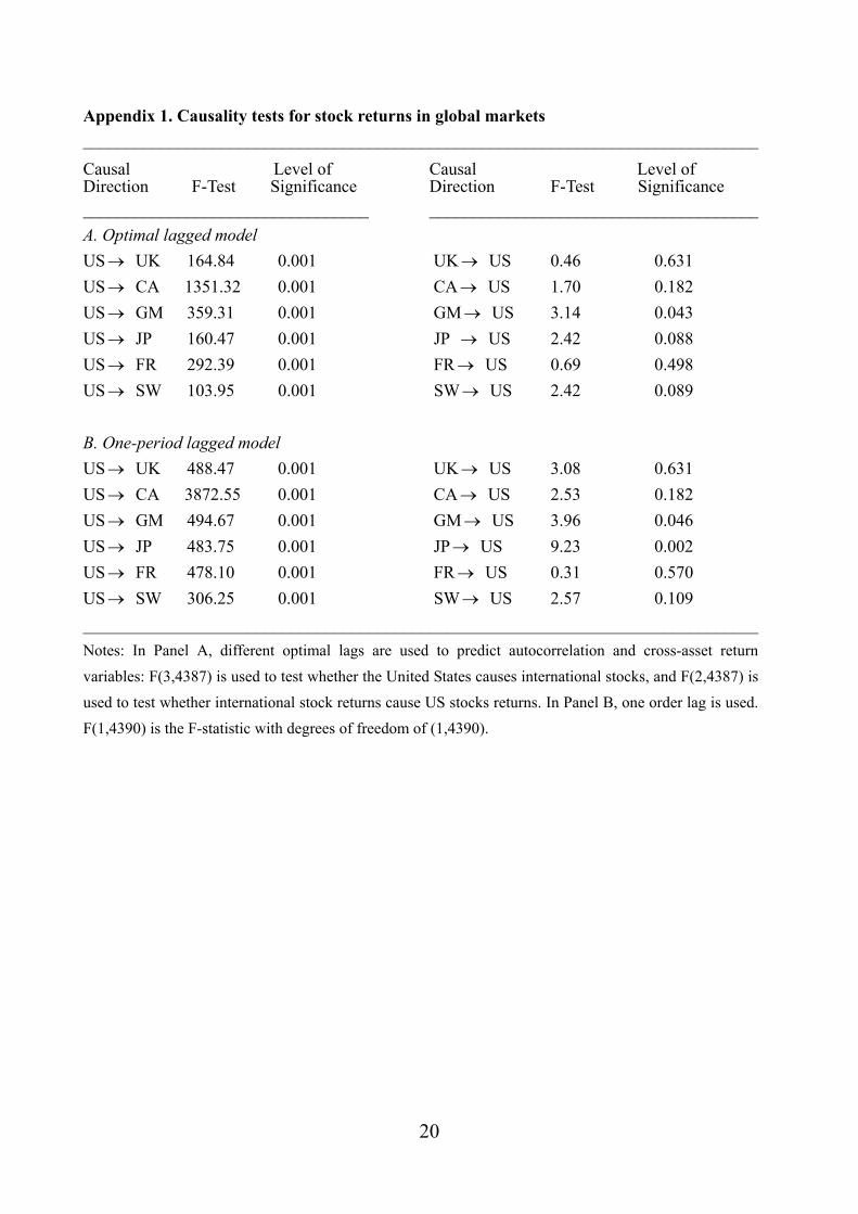
Appendix 1. Causality tests for stock returns in global markets ______________________________________________________________________________

Causal Level of Causal Level of Direction F-Test Significance Direction F-Test Significance _________________________________ ______________________________________ A. Optimal lagged model US UK 164.84 0.001 UK US 0.46 0.631 → →US CA 1351.32 0.001 CA→ US 1.70 0.182 →US GM 359.31 0.001 GM US 3.14 0.043 → →US JP 160.47 0.001 JP US 2.42 0.088 → →US FR 292.39 0.001 FR→ US 0.69 0.498 →US SW 103.95 0.001 SW US 2.42 0.089 → → B. One-period lagged model US UK 488.47 0.001 UK US 3.08 0.631 → →US CA 3872.55 0.001 CA→ US 2.53 0.182 →US GM 494.67 0.001 GM US 3.96 0.046 → →US JP 483.75 0.001 JP US 9.23 0.002 → →US FR 478.10 0.001 FR→ US 0.31 0.570 →US SW 306.25 0.001 SW US 2.57 0.109 → →______________________________________________________________________________ Notes: In Panel A, different optimal lags are used to predict autocorrelation and cross-asset return variables: F(3,4387) is used to test whether the United States causes international stocks, and F(2,4387) is used to test whether international stock returns cause US stocks returns. In Panel B, one order lag is used. F(1,4390) is the F-statistic with degrees of freedom of (1,4390).

20

Appendix 2. Bayesian estimation of the double-threshold model

The system of the Double-Threshold GARCH model in the text is given by:

R = it

>+++

≤+++

−+−+−

−+−+−

,,

,

)2(11

)2(1

)2(0

)1(11

)1(1

)1(0

rRRR

rRRR

jdmtt

jdmt

it

jdmtt

jdmt

it

εψφφ

εψφφ

= th

>++

≤++

−+−−

−+−−

,,

,

1)2(

12

1)2(

1)2(

0

1)1(

12

1)1(

1)1(

0

rRh

rRh

jdmttt

jdmttt

βεαα

βεαα

where the distribution of tε is conditional on information up to time t-1 is N(0, ht). Let kπ be

the time index of the kth smallest observation of {R 1 ,··· ,R n }. Using the time index, we write

the likelihood function as:

j j

∝ ( 2)|( ΘYp Π=

n

t 2thπ )-1/2

−−−− −−=∑ 2

1)1(

11)1(

1)1(

01

)(121 ji

s

k

i

tkkk

RRRh πππ ψφφexp ×

−−−− −−

−

+=∑ 2

1)2(

11)2(

1)2(

0

1

1

)(121exp ji

n

sk

i

tkkk

RRRh πππ ψφφ ,

where is the likelihood function in the sampling process for all observations. Given the

parameters being divided into two different regimes by the threshold variable, r; s satisfies the

restriction

)|( ΘYp

R jsπ d− ≤ r < R . We define Y = ( )’, the unknown parameters j

dk 1+−πiii

nRRR πππ ...,,

21

Θ = ( . )',,,,,,,,,,,,, )2(1

)2(1

)2(0

)2(1

)2(1

)2(0

)1(1

)1(1

)1(0

)1(1

)1(1

)1(0 drβααψφφβααψφφ

To perform the Bayesian analysis of the double TAR-GARCH model, we choose the

following prior distribution for :Θ

),()1,0()1,0()( )2(1

)2(1

)2(0

)1(1

)1(1

)1(0 braIIIp <<⋅<+>⋅<+>∝Θ βααβαα

21

where I (.) is the indicator function that I (A) = 1 if the event A is true and a and b are 25 and 75

percentiles of the threshold variables R t , respectively. The posterior distribution is

then given by the Bayesian rule as:

j )|( Yp Θ

∝ . )|( Yp Θ )()|( Θ⋅Θ pYp

We generate an approximated sample from the posterior distribution by using

Markov chain, Monte Carlo (MCMC) methods, where M is the number of ‘burn-in’ iterations for

convergence and N is the total number of iterations. In our study, M = 10,000 and N =20,000.

The sampling is done in six blocks:

NM ΘΘ + ,...,1

(1) Sample ( from ),, )1(1

)1(1

)1(0 ψφφ ),,|,,(

),,()1(

1)1(

1)1(

0 )1(1

)1(1

)1(0 ψφφ

ψφφ−

ΘYp

(2) Sample ( from ),, )1(1

)1(1

)1(0 βαα ),,|,,(

),,()1(

1)1(

1)1(

0 )1(1

)1(1

)1(0 βαα

βαα−

ΘYp

(3) Sample ( from ),, )2(1

)2(1

)2(0 ψφφ ),,|,,(

),,()2(

1)2(

1)2(

0 )2(1

)2(1

)2(0 ψφφ

ψφφ−

ΘYp

(4) Sample ( from ),, )2(1

)2(1

)2(0 βαα ),,|,,(

),,()2(

1)2(

1)2(

0 )2(1

)2(1

)2(0 βαα

βαα−

ΘYp

(5) Sample r from ),|( rYrp −Θ ,

(6) Sample d from , ),|( dYdp −Θ

where represents the vector without the parameterx−Θ Θ x . Point estimates of any function of

the unknown parameter, say can then be obtained as the sample mean of the posterior

sample. Thus, the point estimate of is given by:

),Θ(f

∧

Θ

= ∧

ΘMN −

1 ∑+=

ΘN

Mk

k

1

.

With respect to the estimated , it is the value occurring most frequently in the posterior sample.

Full details on how to implement the MCMC methods can be found in Chib and Greenberg (1995),

Chen (1998), and Chen and So (2002).

d

22

References

Amihud, Y. and Mendelson, H. 1987. Trading mechanisms and stock returns: an empirical investigation. Journal of Finance 42: 533-553.

Arshanspalli, B., Doukas, J., and Lang, L.H.P. 1997. Common volatility in the industrial structure of global capital markets. Journal of International Money and Finance 16, 189-209.

Bekaert, G. and Wu, G. 2000. Asymmetric volatility and risk in equity markets. The Review of Financial Studies 13: 1-42,

Baillie, R. T. and DeGennaro, R. P. 1990. Stock returns and volatility. Journal of Financial and Quantitative Analysis 25: 203-215.

Becker, K.G, Finnerty, J.E., and Friedman, J.E. 1995. Economic news and equity market linkages between the US and U.K. Journal of Banking and Finance 19: 1191-1210.

Bollerslev, T., Chou, R. Y., and Kroner, K. F. 1992. ARCH modeling in finance: a review of the theory and empirical evidence. Journal of Econometrics, 52: 5-59.

Campbell, J. Y. and Hamao. Y. 1992. Predictable stock returns in the United States and Japan: A study of long-term capital market integration. Journal of Finance, 47: 43-69.

Chen, C.W.S. 1998. A Bayesian analysis of generalized threshold autoregressive models. Statistics and Probability Letters 40: 15-22.

Chen, C.W.S. and So, M.K.P. 2002. On a threshold heteroscedastic model. Working manuscript.

Chiang, T.C. 1998. Stock returns and conditional variance-covariance: evidence from Asian stock markets. J. J. Choi & J. A. Doukas (Eds.), Emerging Capital Markets: Financial and Investment Issues (pp. 241-252). Westport, CN: Quorum Books.

Chiang, T.C. and Chiang, J. 1996. Dynamic analysis of stock return volatility in an integrated international capital market. Review of Quantitative Finance and Accounting 6: 5-17.

Chiang, T. C. and Doong, S. C. 2001. Empirical analysis of stock returns and volatilities: evidence from seven Asian stock markets based on TAR-GARCH model. Review of Quantitative Finance and Accounting 17: 301-318.

Chib, S. and Greenberg, E. 1995. Markov chain Monte Carlo simulation methods in econometrics. Manuscript, Olin School of Business, Washington University in St. Louis.

Cheung, Y-C. and Ng, L. 1992. Stock price dynamics and firm size: an empirical investigation. Journal of Finance 47: 1885-1997.

Connolly, R.A. and Wang, F.A. 2003. International equity market comovements: economic fundamentals or contagion? Pacific-Basin Finance Journal, 11: 23-43.

Damodaran, A. 1993. A simple measure of price adjustment coefficients. Journal of Finance 48: 387-400.

Engle, R.F. and Ng, V.K. 1993. Measuring and testing the impact of news on volatility. Journal of

23

Finance 48: 1749-1778.

Eun, C.S and Shim, S. 1989. International transmission of stock market movements. Journal of Financial and Quantitative Analysis 24: 241-256.

Glosten, L.R., Jagannathan, R., and Runkle, D. 1993. On the relation between the expected value and the volatility of the nominal excess return on stocks. Journal of Finance, 48: 1779-1801.

Green, P. J. 1995. Reversible jump Markov chain Monte Carlo computation and Bayesian model determination. Biometrika 82: 711-732.

Greene, W.H. 2000. Econometric Analysis, Upper Saddle River, NJ: Prentice-Hall.

Hamao, Y., Masulis, R., and Ng, V. 1990. Correlations in price changes and volatility across international stock markets. The Review of Financial Studies 3: 281-307.

Ito, T.R., Engle, R.F., and Lin,W. 1992. Where does the meteor shower come from? The role of stochastic policy coordination. Journal of International Economics 32: 221-240.

Jeon, B. and Chiang, T. 1991. A system of stock prices in world stock exchanges: Common stochastic trends for 1975-1990? Journal of Economics and Business, 43: 329-338.

Johansen, S. 1988. Statistical analysis of cointegration vectors,” Journal of Economic Dynamics and Control, 12: 231-254.

Johansen, S. 1991. Estimation and hypothesis testing of cointegration vectors in Gaussian vector autoregressive models,” Econometrica 59: 1551-1580.

Karolyi, A., and Stulz, R.M. 1996. Why do markets move together? An investigation of U.S.-Japan stock return comovements, Journal of Finance, 51: 951-986.

Kasa, K. 1992. Common stochastic trends in international stock markets. Journal of Monetary Economics 29: 95-124.

Kim, S. W., and Rogers, J. H. 1995. International stock price spillovers and market liberalization: evidence from Korea, Japan, and the United States. Journal of Empirical Finance 2: 117-133.

King, M.A. and Wadhwani, S. 1990. Transmission of volatility between stock markets. The Review of Financial Studies 3: 5-33.

Koch, P.D. and Koch, T.W. 1991. Evolution in dynamic linkages across daily national stock indexes. Journal of International Money and Finance 10: 231-251.

Koutmos, G. 1999. Asymmetric price and volatility adjustments in emerging Asian stock markets. Journal of Business Finance and Accounting 26: 83-101.

Koutmos, G. 1998. Asymmetries in the conditional mean and the conditional variance: evidence from nine stock markets. Journal of Economics and Business 50: 277-290.

Koutmos, G. 1997. Do emerging and developed stock markets behave alike? Evidence from six Pacific Basin stock markets. Journal of International Financial Markets, Institutions and Money 7: 221-234.

24

25

Koutmos, G. and Booth, G. G. 1995. Asymmetric volatility transmission in international stock markets. Journal of International Money and Finance 14: 747-762.

LeBaron, B. 1992. Sine relations between volatility and serial correlations in stock market returns. The Journal of Business 65: 199-219.

Li, C.W. and Li, W.K. 1996. On a double threshold autoregressive heteroscedastic time series model. Journal of Applied Econometrics 11: 253-274.

Masih, R. and Masih, A.M.M. 2001. Long and short term dynamic causal transmission amongst international stock markets. Journal of International Money and Finance 20: 563-587.

Martens, M. and Poon, S-H. 2001. Returns synchronization and daily correlation dynamics between international stock markets. Journal of Banking & Finance 25: 1805-1827.

Nelson, D.B. 1991. Conditional heteroskedasticity in asset returns: a new approach. Econometrica 59: 347-370.

Roll, R. 1992. Industrial structure and the comparative behavior of international stock market indices. Journal of Finance 47: 1-41.

Sentana, E. and Wadhwani, S. 1992. Feedback traders and stock return autocorrelations: evidence from a century of daily data. The Economic Journal 102: 415-435.

Shen, C.H. and Chiang, T.C. 1999. Retrieving the vanishing liquidity effect - a threshold vector autoregressive model. Journal of Economics and Business 51 (3): 257-277.

So, M.K.P., Chen, C.W.S. and Chen, M-T. 2003. A Bayesian threshold nonlinearity test for financial time series. Working manuscript.

Tsay, R.S. 1998. Testing and modeling multivariate threshold models. Journal of the American Statistical Association 84: 231-240.