asymmetries in stock markets

European Journal of Operational Research 241 (2015) 749–762

Contents lists available at ScienceDirect

European Journal of Operational Research

journal homepage: www.elsevier.com/locate/ejor

Stochastics and Statistics

Asymmetries in stock markets

Peijie Wang a,b,∗, Bing Zhang c, Yun Zhou d

a University of Plymouth, Plymouth PL4 8AA, UKb IÉSEG, Lille 59000, Francec Department of Finance and Insurance, Nanjing University, Nanjing 210093, PR Chinad International College, China Agricultural University, Beijing 100083, PR China

a r t i c l e i n f o

Article history:

Received 24 June 2013

Accepted 1 September 2014

Available online 18 October 2014

Keywords:

Asymmetry

Volatility

Return reversals

Return persistency

a b s t r a c t

This paper analyzes three major asymmetries in stock markets, namely, asymmetry in return reversals,

asymmetry in return persistency and asymmetry in return volatilities. It argues for a case of return persistency

as stock returns do not always reverse, in theory and in practice. Patterns in return-volatility asymmetries

are conjectured and investigated jointly, under different stock market conditions. Results from modeling

the world’s major stock return indexes render support to the propositions of the paper. Return reversal

asymmetry is illusionary arising from ambiguous parameter estimations and deluding interpretations of

parameter signs. Asymmetry in return persistency, still weak though, is more prevalent.

© 2014 Elsevier B.V. All rights reserved.

1

b

a

n

m

(

c

v

t

a

o

e

t

i

s

l

m

s

c

t

v

t

3

m

t

v

r

m

i

p

2

r

v

s

m

s

t

i

v

S

m

i

a

a

m

h

0

. Introduction

While asymmetric time-varying volatility on the stock market has

een widely documented in the empirical literature, the other major

symmetric phenomenon, asymmetry in returns, has yet to be scruti-

ized. Although the former has been publicized with the news argu-

ent, the leverage notion and even an econometric model of EGARCH

Exponential General Autoregressive Conditional Heteroskedasticity,

f. Nelson 1991), the latter is more direct in shaping returns to in-

estors. Further, interactions between return and volatility asymme-

ries need to be probed into, to identify the right source of asymmetry

nd to avoid the delusion of one kind of asymmetry in the name of the

ther. Critically, most empirical studies have overlooked the differ-

nce between a shock to stock returns and the return itself, thereby

he terminology of asymmetry in return reversals has emerged, which

s at most half of the veracities. During stock market upturns, both

lope and intercept parameters in the mean (return) equation are

ikely to be positive, so positive returns persist and negative returns

ay tend to reverse, regardless of a positive or negative past return

hock. The present study proposes hypothetically and tests empiri-

ally this new strand of asymmetry, i.e., return persistency asymme-

ry, alongside return reversal asymmetry and their interactions.

The rest of the paper progresses as follows. The next section pro-

ides a brief review and discussion of recent research on asymme-

ries in stock return reversals and volatilities. Section 3 specifies the

∗ Corresponding author at: IÉSEG, Lille 59000, France. Tel.: +44 1752 585705/+33

20 545 892.

E-mail address: [email protected], [email protected] (P. Wang).

S

1

s

(

B

ttp://dx.doi.org/10.1016/j.ejor.2014.09.029

377-2217/© 2014 Elsevier B.V. All rights reserved.

odels and develops the corresponding hypotheses. It elaborates on

he behavioral patterns in return reversal/persistency asymmetry and

olatility asymmetry, vis-à-vis the restrictions imposed on the return

eversal/persistency asymmetry parameters and the volatility asym-

etry parameters. Section 4 presents the empirical results and find-

ngs of this study, with further deliberation on the implications of the

resent study. Finally, Section 5 summarizes this study.

. Asymmetries in stock return reversals and volatilities

It has been widely documented that a negative shock to stock

eturns, or an unexpected fall in the stock price, tends to increase

olatility of the stock to a greater extent than a positive shock to

tock returns, or an unexpected rise in the stock price of the same

agnitude. This kind of volatility asymmetry exhibits asymmetric re-

ponses to good news vis-à-vis bad news, and is reasonably attributed

o, and explained by, the leverage effect in the literature. It is not the

ntention of the present paper to review this kind of asymmetry in

olatilities, which is abundant in the literature ready to be referred to.

tudies on return reversals, or stock market overreactions and asym-

etries in stock market returns, include De Bondt and Thaler (1985)

n early days, which continues to progress and one of the recent ex-

mples is Kedar-Levy, Yu, Kamesaka, and Ben-Zion (2010). De Bondt

nd Thaler (1985) have found that investors overreact on the stock

arket, using monthly returns on the stocks listed on the New York

tock Exchange for the period between January 1926 and December

982. Their results and findings are confirmed or supported by later

tudies by Zarowin (1989,1990), Dissanaike (1996), Kim and Nelson

1998), Malliaropulos and Priestley (1999), Atkins and Dyl (1990) and

remer and Sweeney (1991), Iihara, Kato, and Tokunaga (2004), and

http://dx.doi.org/10.1016/j.ejor.2014.09.029

http://www.ScienceDirect.com

http://www.elsevier.com/locate/ejor

http://crossmark.crossref.org/dialog/?doi=10.1016/j.ejor.2014.09.029&domain=pdf

mailto:[email protected]

mailto:[email protected]

http://dx.doi.org/10.1016/j.ejor.2014.09.029

750 P. Wang et al. / European Journal of Operational Research 241 (2015) 749–762

Table 1

Persistency and reversal patterns: Rt = μ0 + μ1Rt−1 + εt .

μ0 0 + − + − + − 0

μ1 + + + 0 0 − − −

Rt−1 > 0 Persist Persist Mixed Persist Reverse Mixed Revers Reverse

Rt−1 < 0 Persist Mixed Persist Reverse Persist Reverse Mixed Reverse

w

r

m

r

a

t

a

n

P

t

v

p

m

m

t

a

t

a

h

a

s

v

v

t

H

t

o

g

t

b

s

m

m

m

n

a

a

t

i

r

r

t

m

i

t

t

K

t

r

(

t

p

r

r

i

Nam, Pyun, and Avard (2001). Recently, Hwang and Rubesam (2013)

provide an explanation to overreactions and asymmetries in stock re-

turns based on behavioral biases. Two conditions that increase return

reversals are proposed. Return reversals increase when investors re-

spond to public signals asymmetrically or when public signals become

noisy.

Most empirical studies, however, have overlooked the difference

between a positive (negative) shock to stock returns and a positive

(negative) return itself. Their results and findings may look sound

with return data in stock market downturns or stagnation, but are

questionable otherwise. Failing to differentiate shocks to returns

and returns themselves would mingle persistence with reversion.

These can be demonstrated with a basic model for capturing rever-

sion, Rt = μ0 + μ1Rt−1 + εt . During booming times or stock market

upturns, both slope and intercept parameters in the mean (return)

equation are likely to be positive, so a positive past return tends to

persist, regardless of a positive or negative past return shock. Whereas

negative past return could either persist or reverse, depending on the

relative size of the intercept and slope parameters. Table 1 summa-

rizes the return persistency/reversal patterns of positive and negative

past returns, given assorted combinations of the intercept and slope

parameters. The table is arranged with return persistency decreas-

ing/return reversals increasing from left to right, starting with the

highest return persistency tendency case and ending with the highest

return reversal tendency case. It can be observed that no clear pat-

terns of persistency/reversals exist in many cases, even less unlikely

for asymmetry in return persistency/reversals. Return reversals may

apply to stock market downturns, during which the slope parameter

is likely to be negative. When stock prices stagnate, the slope param-

eter can be negative with a positive intercept, or be positive with a

negative intercept, and the former case could exhibit mean reversion

tendencies. As returns do not always reverse, we study whether stock

returns would persist with a higher compounding rate following a

positive return shock as against a negative return shock.

There are a few real and behavioral factors that may possibly

induce asymmetry in return persistency and reversals. In booming

times, the stock price is on average rising around an up sloping trend.

A positive past return shock coupled with a positive past return means

that, while the expectation was on the rise, it was not higher enough

in the previous round. Whereas a negative past return shock cou-

pled with a positive past return indicates that investors were over

optimistic. Positive stock returns are therefore more likely to persist

and to persist to a higher degree in the former than in the latter. The

catchphrase “a good round deserves another” probably best explains

this asymmetry pattern. Then it comes to the case of a negative past

return. Stock returns would reverse to a larger degree with a positive

past return shock, vis-à-vis a negative past return shock, under our

framework. i.e., stock returns would become positive or lesser nega-

tive following a positive return shock, but remain negative or deeper

negative following a negative return shock. The conventional propo-

sitions and analysis in return reversals in the existing literature would

work appropriately in stock market downturns, nevertheless. With a

negative slope parameter under the circumstances, stock returns al-

most always reverse. With the expectations that stock performance

improves more or deteriorates less following a positive return shock

than a negative return shock, there would be the following patterns in

return reversal asymmetry. Experiencing a positive past return shock,

stock returns would reverse to a lesser extent when the past return

as positive, and would reverse to a larger extent when the past

eturn was negative, both being an indication of improving perfor-

ance or recovery. Whereas given a negative past return shock, stock

eturns reverse to a larger extent with a positive past stock return

nd to a lesser extent with a negative past stock return, both being

he indication of deteriorating performance or relapse.

Few studies have included both asymmetric return reversals

nd asymmetric time-varying volatilities in empirical investigations,

onetheless. Adopting an ANST-GARCH modeling approach, Nam,

yun, and Avard (2002) study asymmetric mean reversion and con-

rarian profits, so both asymmetries in mean reversion and time-

arying volatilities can be examined. Koutmos (1998) tests the hy-

othesis for nine national stock markets that both the conditional

ean and the conditional variance of stock index returns are asym-

etric functions of past information. The empirical evidence suggests

hat both the conditional mean and the conditional variance respond

symmetrically to past information. He alleges that asymmetry in

he conditional mean is linked to asymmetry in the conditional vari-

nce, because the faster adjustment of prices to bad news causes

igher volatilities during down markets, which suggest that volatility

symmetry increases with mean reversion asymmetry. Park (2011)

uggests that asymmetric herding is a source of asymmetric return

olatility. His work is based on exchange rate data though and in-

olves no asymmetries in return reversals. Charles (2010) has found

hat asymmetry influences the day-of-the-week effect on volatility.

ua and Zhang (2008) deal with asymmetry in conditional distribu-

ion and volatility asymmetry. It is claimed that empirical results of

ne-step-ahead density forecasts on the weekly S&P500 returns sug-

est that forecast quality can be significantly improved by modeling

hese asymmetric features.

Recently, Wang and Wang (2011) have scrutinized the interactions

etween return reversal asymmetry and volatility asymmetry. They

uggest that mean reversion asymmetry and volatility asymmetry

ay originate from similar sources and causes but the two asym-

etries do not reinforce each other. Volatility asymmetry can be a

easure of ambiguity in mean reversion asymmetry. There would be

o or weak volatility asymmetry, instead of strong, definite volatility

symmetry, when there is a strong, clear pattern of mean reversion

symmetry. They argue that asymmetric return reversals can be bet-

er explained by risk aversion functions where relative risk aversion

s a decreasing function of wealth levels, or conditional on the di-

ection of changes in wealth levels. This asymmetry in risk premium

equirements could be the source of asymmetry in return reversals

hat would otherwise have been symmetric. They propose that asym-

etry in variances is the residual effect of mean reversion asymmetry

n the interaction between the mean and the variance, in terms of the

rade-off between asymmetry in return reversals and asymmetry in

ime-varying volatilities. Their empirical results contradict those in

outmos (1998).

Different from all the previous research, the present study scru-

inizes return persistency asymmetry in exploiting the mystery in

eturn behavior and patterns. It is in contrast to Wang and Wang

2011) and Koutmos (1998) who have associated the two asymme-

ries in return reversals and in volatilities to a certain extent. The

resent study makes inquiries into whether and how asymmetry in

eturn reversals and persistency surfaces. The study examines return

eversal/persistency asymmetry and volatility asymmetry jointly and

n a balanced way, imposing no prior conditions on the likely patterns

P. Wang et al. / European Journal of Operational Research 241 (2015) 749–762 751

i

a

t

c

3

a

t

i

t

o

n

R

t

m

v

a

i

s

p

R

w

a

p

d

f

v

a

M

R

p

g

t

t

r

l

r

a

a

i

s

s

f

M

W

εt

s

λr

r

ρr

a

e

w

t

f

e

t

h

W

V

θi

s

V

S

a

εc

a

a

g

t

n

f

s

v

t

σ

w

t

R

h

E

s

t

o

M

i

f

a

i

p

H

t

a

o

H

t

s

t

I

p

R

h

f

m

n return reversal/persistency asymmetry and volatility asymmetry

nd restrict to no specific geographical regions. It distinguishes the

wo asymmetries on the ground of their underpinning makings with

orresponding model specifications and hypothesis tests.

. Models and hypotheses

We model the proposed return persistency asymmetry, along with

symmetries in stock return reversals and stock return volatilities in

his section. Both return reversal/persistency asymmetry and volatil-

ty asymmetry are modeled with a threshold function and a smooth

ransition function, accommodating diverse views on the properties

f the two processes. Restrictions are further imposed on the perti-

ent parameters of the model in relation to the test of the proposition.

eturn reversal/persistency asymmetry features the qualitative reac-

ion to the sign of the shock; whereas volatility itself responds to the

agnitude of previous shocks that are quantitative measures, so does

olatility asymmetry. Volatility is proportional to the size of either

positive shock or a negative shock, but the ratio of proportionality

s hypothesized to be higher for a negative shock than for a positive

hock with equal size. Eq. (1) below is the general model for the mean

rocess:

t = μ0 + M(εt−1)Rt−1 + εt (1)

here Rt is return on the stock, εt is the residual, and μ0, μ1, ρre coefficients. M(εt−1) captures asymmetry in mean reversion or

ersistency. Two types of design for M(εt−1) are adopted. One is the

ummy variable approach and the other assumes a kind of transition

unction. For the former, an endogenous dummy variable takes the

alue of unity if the residual or shock in the previous period is negative

nd zero otherwise, capturing asymmetry in mean reversion:

(εt−1) = μ1 + ρD(εt−1) ={μ1 + ρ, εt−1 < 0,

μ1, εt−1 ≥ 0(2)

eturns reverse when μ1 is negative. The sign of ρ is negative in the

resence of asymmetry of mean reversion, i.e., returns reverse to a

reater extent following a negative return shock. If μ1 is positive,

hen returns do not reverse but persist following a positive past re-

urn shock. Given a ρ in the range of −μ1 < ρ < 0, or μ1 + ρ > 0,

eturns still persist following a negative past return shock, but with a

ower compounding rate. Only when ρ < −μ1, or μ1 + ρ < 0, would

eturns reverse following a negative past return shock. Overall, a neg-

tive ρ indicates return reversal asymmetry that returns reverse to

greater extent following a negative past return shock. Likewise,

t indicates return persistency asymmetry that returns tend to per-

ist with a higher compounding rate following a positive past return

hock.

A logistic type specification is assumed for the design of transition

unctions:

(εt−1) = μ1 + ρ[1 + exp(−λεt−1)]−1 (3)

ith λ < 0, M(εt−1) → μ1 when εt−1 → ∞, M(εt−1) → μ1 + ρ when

t−1 → −∞ and M(εt−1) → μ1 + 0.5ρ when εt−1 → 0. When λ > 0,

he function value mirrors that for the M(εt−1) → μ1 case. λ mea-

ures the degree of smoothness of the transition function. A larger

in absolute value corresponds to a sharper asymmetry in return

eversals/persistency. In its extremity, an infinite λ in absolute value

educes the logistic function to a threshold function. It is required that

and λ have the same sign for the null of our hypothesis regarding

eturn reversal/persistency asymmetry, i.e., ρ < 0 and λ < 0 or ρ > 0

nd λ > 0. Whereas both sets of requirements are equivalent math-

matically, the latter set of requirements is inclined to be associated

ith return persistency asymmetry.

Asymmetry in time-varying volatilities is also specified by a

hreshold function and a smooth transition function that will be tested

or superiority empirically. Adopting a most parsimonious as well as

ffective GARCH(1,1) for the symmetric part of time-varying volatili-

ies, the general model for the variance process is as follows:

t = (α0 + α1ε

2t−1 + β1ht−1

)V(εt−1) (4)

ith a threshold specification, V(εt−1) takes the form of:

(εt−1) = 1 + θD(εt−1) ={

1 + θ, εt−1 < 01, εt−1 ≥ 0

(5)

> 0 is required for the kind of volatility asymmetry where volatility

s greater following a negative return shock than a positive return

hock. The logistic specification is as follows:

(εt−1) = 1 + θ [1 + exp(−γ εt−1)]−1 (6)

imilar to the cases for asymmetry in mean revision/persistence

nd with γ < 0, V(εt−1) → 1 when εt−1 → ∞, V(εt−1) → 1 + θ when

t−1 → −∞ and V(εt−1) → 1 + 0.5θ when εt−1 → 0 for both specifi-

ations. If γ > 0, the function value mirrors that for the γ < 0 case. θnd γ are required to possess opposite signs for exhibiting a volatility

symmetry pattern consistent to our hypothesis. γ measures the de-

ree of volatility asymmetry, a larger γ in absolute value corresponds

o a higher degree of volatility asymmetry. In extreme cases, an infi-

ite γ in absolute value reduces the logistic function to a threshold

unction.

Let us consider briefly the stationarity conditions for the above

pecified variance. Notice that E {V(εt−1)} = 1 + 0.5θ for all the two

ariance specifications of Eqs. (5) and (6). Therefore, taking expecta-

ions operation for Eq. (4) gives rise to:

2ε = (

α0 + α1σ2ε + β1σ

2ε

)(1 + 0.5θ) (7)

here σ 2ε is the unconditional variance of the residual. It follows that

he stationarity conditions are:

α1 + β1 <1

1 + 0.5θ(8)

The joint mean and variance function are expressed as follows:

t = μ0 + M(εt−1)Rt−1 + εt

t =(α0 + α1ε

2t−1 + β1ht−1

)V(εt−1)

(9)

q. (9) is the general model and the base upon which various re-

trictions will be imposed to test our hypotheses empirically. No-

ice that the mean reversion/persistence asymmetry specification

f Eq. (3) encompasses that of Eq. (2). It can be observed that

(εt−1) → μ1 + ρD(εt−1

)when λ → −∞ for εt−1 �= 0. Next, there

s no mean reversion/persistence asymmetry if ρ = 0 is confirmed

or the specification in Eq. (2) or Eq. (3). Correspondingly, there

re following hypotheses to be tested empirically, with regard to

mposing restrictions on the return reversal/persistency asymmetry

arameters:

1. Return reversal/persistency asymmetry is a quantitative response

o the previous return shock. The null of the hypothesis is −∞ < λ < 0

nd ρ < 0 or 0 < λ < ∞ and ρ > 0 with the smooth transition process

f Eq. (3).

2. Return reversal/persistency asymmetry is a qualitative response to

he sign of the previous return shock. The null of the hypothesis for the

pecification of Eq. (3) is λ → −∞ and ρ < 0 or λ → ∞ and ρ > 0, and

he null is ρ < 0 with the threshold process of Eq. (2).

mposing restrictions on the mean reversion/persistence asymmetry

arameter in Eq. (3) leads to the following model, called MM1:

t = μ0 + [μ1 + ρD (εt−1)] Rt−1 + εt

t =(α0 + α1ε

2t−1 + β1ht−1

)V(εt−1)

(10)

or testing H1. Further, there is no mean reversion/persistence asym-

etry if H2 is rejected, and the restricted model, named MM2, takes


c

w

a

w

m

n

4

d

s

A

m

i

f

a

s

1

t

t

l

t

F

t

o

m

r

s

A

t

2

f

l

b

M

T

i

t

k

T

e

k

w

a

J

p

G

M

i

T

a

f

w

a

b

2

a

1

E

a

p

M

s

the following form:

Rt = μ0 + μ1 Rt−1 + εt

ht =(α0 + α1ε

2t−1 + β1ht−1

)V(εt−1)

(11)

Similar restrictions are imposed on the variance asymmetry pa-

rameters, with the following corresponding hypotheses:

H3. There exists asymmetry in time-varying volatilities that is a quali-

tative response to the previous return shock. The null of the hypothesis

is γ → −∞ and θ > 0 or γ → ∞ and θ < 0 with the specification of

Eq. (6). The null of the hypothesis is θ > 0 with the specification of

Eq. (5).

H4. There exists asymmetry in time-varying volatilities that is a quan-

titative function of the previous return shock, i.e., it responds to both the

size and the sign of the previous return shock. The null of the hypothesis is

−∞ < γ < 0 and θ > 0 or 0 < γ < ∞ and θ < 0 with the specification

of Eq. (6).

It is expected that the null of H4 would be preferred to the null of

H3 according to the previous analysis and reasoning. Failing to reject

the null of H3, i.e., the variance specification of Eq. (6) is not found

to be superior to the variance specification of Eq. (5), leads to the

following model, named MV1:

Rt = μ0 + M(εt−1)Rt−1 + εt

ht =(α0 + α1ε

2t−1 + β1ht−1

)[1 + θD(εt−1)]

(12)

That is, there is asymmetry in time-varying volatilities but it follows

a threshold process rather than a smooth transition process. Further

there is no any kind of asymmetry in volatilities if the restriction θ = 0

is valid, or the null of H3 is rejected. The resulting model, named MV2,

is as follows:

Rt = μ0 + M(εt−1)Rt−1 + εt

ht = α0 + α1ε2t−1 + β1ht−1

(13)

The above hypotheses deal with asymmetries in return persis-

tency/reversals and volatilities individually. As stressed earlier, one

of the issues is the interactions between the two asymmetries.

Conceptualizing the discussions in the previous section, we put for-

ward two additional hypotheses, the ambiguity hypothesis and illu-

sion hypothesis, as follows:

H5. Return reversal/persistency asymmetry is ambiguous. The null of

the hypothesis is ρ = 0 with the specification of Eq. (2) or Eq. (3); or the

B,T specification is not statistically superior to the N,T specification in the

tables.

H6. Return reversal/persistency asymmetry is illusionary.

There are two parts for this hypothesis as follows:

H6a. It is illusionary that suppressing the volatility asymmetry param-

eter deteriorates the performance of the model while inducing asymme-

try in return revision/persistence in the mean equation. The null of the

hypothesis is a significant log likelihood ratio test statistic, LR, for the

specification of Eq. (13) versus the specification of Eq. (9); meanwhile,

asymmetry in return revision/persistence is induced, i.e., ρ = 0 with

Eq. (9) becomes ρ �= 0 after suppressing the volatility asymmetry pa-

rameter incorrectly with Eq. (13).

H6b. It is illusionary that adopting over sophisticated specifications does

not improve on model performance while conceiving asymmetry in re-

turn revision/persistence in the mean equation. The null of the hypothesis

is an insignificant log likelihood ratio test statistic, LR, for the full spec-

ification versus the specification of Eq. (10) and Eq. (11); or the T,T

specification is not statistically superior to the B,T and N,T specifications

in the tables. Meanwhile, asymmetry in return revision/persistence is

onceived, i.e., ρ = 0 with the B,T specification becomes ρ �= 0, λ �= 0

ith the T,T specification.

Attempts to predict returns based on return reversal/persistency

symmetry parameter values, which are rather unconfirmed, end up

ith making even larger prediction errors on some occasions while

aking smaller prediction errors on some other occasions, achieving

o overall improvements.

. Data, results and discussions

The data sets used in this study are FTSE All World return in-

ex and its eight constituency indexes, comprising the geographical

preads of Asia Pacific, North America, Latin America, Middle East and

frica, Europe, and the development stage groupings of all emerging

arkets, advanced emerging markets, and developed markets. All the

ndexes are measured in the US dollars. In addition, the return index

or the euro area is included, denominated in both the US dollars

nd the euros. So, there are 11 return series in total covered in this

tudy. The data sets span 15 years, starting on Wednesday January 1,

997 and ending on Friday December 2011, yielding 3913 observa-

ions in total for each of the return series. The period encompasses

wo major financial crises, the Asian financial crisis in 1997 and the

atest global financial crisis triggered by a complex interplay of valua-

ion and liquidity problems in banking and financial systems in 2008.

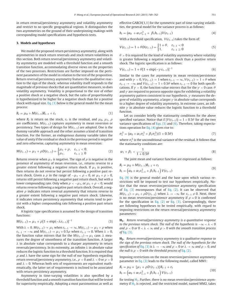
ig. 1 illustrates stock market movements in this period, choosing

hree markets out of 11 with representative patterns. They are devel-

ped markets, all emerging markets, and Asia Pacific. The developed

arket is hit little by the 1997 Asian financial crisis but has expe-

ienced a major downturn from the turn of the millennium to the

pring in 2003. In contrast, the emerging market is hit hard by the

sian financial crisis and has experienced a significant downturn be-

ween June 1997 and October 1998, and stagnated until the spring of

003. Then the stock market around the globe has enjoyed an over

our years’ booming era until the end of October 2007. It is then fol-

owed by the most severe stock market plummet in 80 years triggered

y the US subprime mortgage crisis. The market has recovered from

arch 2009 but is hit again in May 2011 by the Greek debt crisis.

he markets in North America, Europe and the euro area measured

n both the US dollars and the euros share the same pattern as that in

he developed market. So does the all world index as developed mar-

ets still play a dominant role on the stage of global stock markets.

he markets of Middle East and Africa, Latin America and advanced

merging economies bear the hallmark of that of all emerging mar-

ets. Whereas the markets in Asia Pacific share the similar pattern

ith emerging markets during the 1997 Asian financial crisis period

nd with developed markets in the stock market downturn between

anuary 2000 and March 2003, due to the fact that Asia Pacific encom-

asses both merging markets and developed markets such as Japan.

iven these patterns in stock market movements, the period between

arch 12, 2003 and October 31, 2007 is set to be the major boom-

ng period for empirical analysis in this study, for all return indexes.

he sharp downturn period from October 31, 2007 to March 9, 2009 is

lso experienced by all return indexes, so is an auxiliary upturn period

rom March 9, 2009 to May 2, 2011. For the markets in the developed

orld, North America, Europe, the euro area and the all world, there is

n additional auxiliary upturn period from January 1, 1997 to Decem-

er 31, 1999; and the period between January 1, 2000 and March 12,

003 is the major downturn period. For advanced emerging markets,

ll emerging markets and Asia Pacific, the period between June 26,

997 and October 5, 1998 is an auxiliary downturn period. For Middle

ast and Africa and Latin America, the period between January 1, 1997

nd March 12, 2003 is reserved for stack market stagnation. This pa-

er only reports the results for (a) the major booming period between

arch 12, 2003 and October 31, 2007 for all return indexes, (b) The

harp downturn, or the financial crisis, period from October 31, 2007


0

100

200

300

400

500

600

700

800

900

01/01/1997 01/01/1999 01/01/2001 01/01/2003 01/01/2005 01/01/2007 01/01/2009 01/01/2011

All Emerging Markets

0

50

100

150

200

250

300

350

400

01/01/1997 01/01/1999 01/01/2001 01/01/2003 01/01/2005 01/01/2007 01/01/2009 01/01/2011

Asia Pacific Markets

(a)

(b)

(c)

Fig. 1. Stock market movement.

t

d

t

a

M

i

p

n

a

u

d

w

s

m

s

f

m

i

s

o March 9, 2009 also experienced by all return indexes, (c) the major

ownturn period between January 1, 2000 and March 12, 2003 for

he developed world, North America, Europe, the euro area and the

ll world, and (d) the stagnation period between January 1, 1997 and

arch 12, 2003 for Middle East and Africa and Latin America.

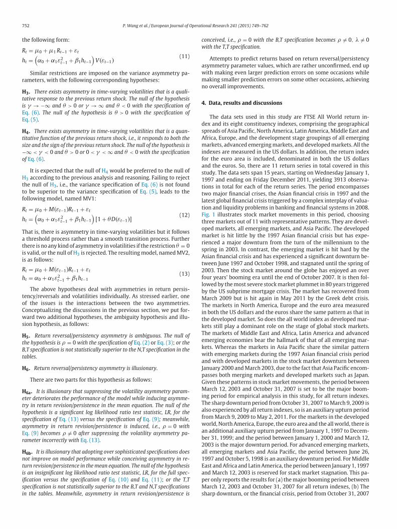
Fig. 2 demonstrates the estimation strategy of this study. Start-

ng with smooth transition specifications for both mean reversion/

ersistence asymmetry and variance asymmetry on the top, perti-

ent restrictions are imposed to inspect whether the specification at

higher level is superior to the specification at the lower level. If the

pper level specification is not superior to the specification one level

own, the estimation process moves down to the next level, other-

ise it stops at the upper level. There are five levels altogether. The

pecification on the top with both mean reversion/persistence asym-

etry and variance asymmetry performs no better than the MM1

pecification in most of the cases. Either the likelihood ratio statistic

or adopting the encompassing model is not significant, or the esti-

ation fails to converge using a variety of algorithms and numbers of

terations. On the other hand, the MV1 specification is inferior to the

pecification with both mean reversion/persistence asymmetry and


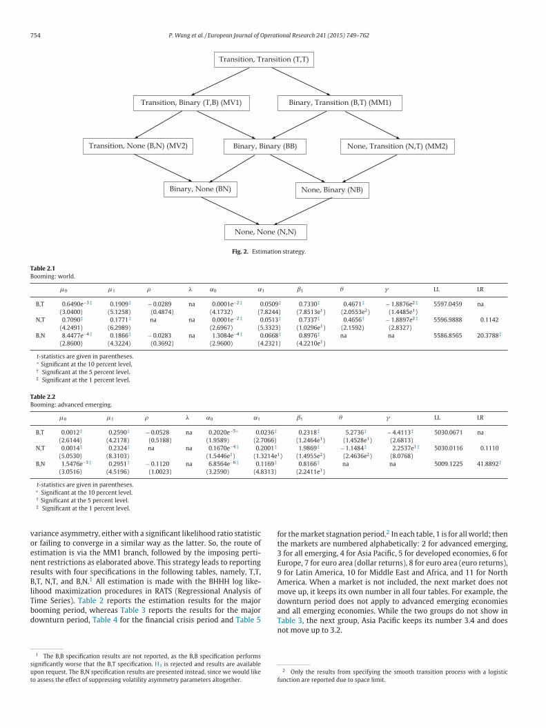
Fig. 2. Estimation strategy.

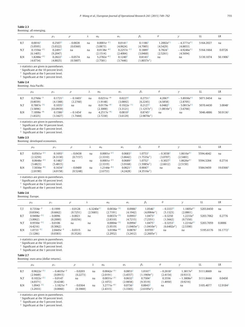
Table 2.1

Booming: world.

μ0 μ1 ρ λ α0 α1 β1 θ γ LL LR

B,T 0.6490e−3‡ 0.1909‡ − 0.0289 na 0.0001e−2‡ 0.0509‡ 0.7330‡ 0.4671‡ − 1.8876e2‡ 5597.0459 na

(3.0400) (5.1258) (0.4874) (4.1732) (7.8244) (7.8513e1) (2.0553e2) (1.4485e1)

N,T 0.7090‡ 0.1771‡ na na 0.0001e−2‡ 0.0513‡ 0.7337‡ 0.4656† − 1.8897e2‡ 5596.9888 0.1142

(4.2491) (6.2989) (2.6967) (5.3323) (1.0296e1) (2.1592) (2.8327)

B,N 8.4477e−4‡ 0.1866‡ − 0.0283 na 1.3084e−4‡ 0.0668‡ 0.8976‡ na na 5586.8565 20.3788‡

(2.8600) (4.3224) (0.3692) (2.9600) (4.2321) (4.2210e1)

t-statistics are given in parentheses.∗ Significant at the 10 percent level.† Significant at the 5 percent level.‡ Significant at the 1 percent level.

Table 2.2

Booming: advanced emerging.

μ0 μ1 ρ λ α0 α1 β1 θ γ LL LR

B,T 0.0012‡ 0.2590‡ − 0.0528 na 0.2020e−5∗ 0.0236‡ 0.2318‡ 5.2736‡ − 4.4113‡ 5030.0671 na

(2.6144) (4.2178) (0.5188) (1.9589) (2.7066) (1.2464e1) (1.4528e1) (2.6813)

N,T 0.0014‡ 0.2324‡ na na 0.1670e−4‡ 0.2001‡ 1.9869‡ − 1.1484‡ 2.2537e1‡ 5030.0116 0.1110

(5.0530) (8.3103) (1.5446e1) (1.3214e1) (1.4955e2) (2.4636e2) (8.0768)

B,N 1.5476e−3‡ 0.2951‡ − 0.1120 na 6.8564e−6‡ 0.1169‡ 0.8166‡ na na 5009.1225 41.8892‡

(3.0516) (4.5196) (1.0023) (3.2590) (4.8313) (2.2411e1)


f

t

3

E

9

A

m

d

a

T

variance asymmetry, either with a significant likelihood ratio statistic

or failing to converge in a similar way as the latter. So, the route of

estimation is via the MM1 branch, followed by the imposing perti-

nent restrictions as elaborated above. This strategy leads to reporting

results with four specifications in the following tables, namely, T,T,

B,T, N,T, and B,N.1 All estimation is made with the BHHH log like-

lihood maximization procedures in RATS (Regressional Analysis of

Time Series). Table 2 reports the estimation results for the major

booming period, whereas Table 3 reports the results for the major

downturn period, Table 4 for the financial crisis period and Table 5

1 The B,B specification results are not reported, as the B,B specification performs

significantly worse that the B,T specification. H3 is rejected and results are available

upon request. The B,N specification results are presented instead, since we would like

to assess the effect of suppressing volatility asymmetry parameters altogether.

n

f

or the market stagnation period.2 In each table, 1 is for all world; then

he markets are numbered alphabetically: 2 for advanced emerging,

for all emerging, 4 for Asia Pacific, 5 for developed economies, 6 for

urope, 7 for euro area (dollar returns), 8 for euro area (euro returns),

for Latin America, 10 for Middle East and Africa, and 11 for North

merica. When a market is not included, the next market does not

ove up, it keeps its own number in all four tables. For example, the

ownturn period does not apply to advanced emerging economies

nd all emerging economies. While the two groups do not show in

able 3, the next group, Asia Pacific keeps its number 3.4 and does

ot move up to 3.2.

2 Only the results from specifying the smooth transition process with a logistic

unction are reported due to space limit.


T

B

141‡

624)

257e−

084)

240‡

446)

T

B

0227‡

0892)

1922e

3121)

0810‡

6129)

T

B

1

0.068

3.864

0.068

3.916

0.062

4.242

T

B

α1

0

(4

0

(4

0

(1

0

(3

T

B

α1

0.08

(3.45

0.06

(2.98

0.07

(3.33

able 2.3

ooming: all emerging.

μ0 μ1 ρ λ α0 α1

B,T 0.0016‡ 0.2507‡ − 0.0028 na 0.0001e−2‡ 0.0

(5.0595) (5.0322) (0.0360) (3.0873) (4.0

N,T 0.1556e−2‡ 0.2491‡ na na 0.0138e−4† 0.2

(6.1405) (9.2047) (2.1514) (2.4

B,N 1.8288e−3‡ 0.2822‡ − 0.0574 na 5.2782e−6‡ 0.1

(4.6734) (4.8825) (0.5807) (2.7581) (3.7


able 2.4

ooming: Asia Pacific.


B,T 0.2760e−3 0.1721‡ − 0.1603† na 0.0251e−4∗ 0.

(0.8039) (4.1388) (2.2760) (1.9148) (3.

N,T 0.7887e−3‡ 0.1035‡ na na 0.0179e−4† 0.

(3.5896) (63.0939) (2.3000) (3.

B,N 7.1898e−4∗ 0.1586‡ − 0.1454∗ na 4.2517e−4‡ 0.

(1.8325) (3.3427) (1.7444) (2.7230) (3.


able 2.5

ooming: developed economies.

μ0 μ1 ρ λ α0 α

B,T 0.0561e−2† 0.1693‡ − 0.0438 na 0.0001e−2†

(2.3259) (8.3130) (0.7157) (2.3310) (

N,T 0.0648e−2‡ 0.1482‡ na na 0.0001e−2†

(3.4823) (5.4815) (2.3319) (

B,N 7.5036e−4‡ 0.1634‡ − 0.0400 na 1.2144e−6‡

(2.8190) (4.0158) (0.5248) (2.6753) (


able 2.6

ooming: Europe.

μ0 μ1 ρ λ α0

T,T 0.7354e−2 − 0.1999 − 0.0128 − 6.3240e1† 0.0036e−3‡

(0.8304) (0.6662) (0.7251) (2.5683) (2.7191)

B,T 0.9498e−3‡ − 0.0096 − 0.0021 na 0.0037e−3‡

(3.0062) (0.2000) (0.0256) (2.8310)

N,T 0.9550e−3‡ − 0.0106 na na 0.0004e−3‡

(4.4216) (0.3062) (5.9519)

B,N 1.0733−3‡ 2.0445e−3 − 0.0315 na 3.0196e−6†

(3.1286) (0.0383) (0.3526) (2.2952)


able 2.7

ooming: euro area (dollar returns).

μ0 μ1 ρ λ α0

B,T 0.9622e−3‡ − 0.4635e−2 − 0.0203 na 0.0042e−3†

(2.9449) (0.0915) (0.2273) (2.0191)

N,T 0.1022e−2‡ − 0.0147 na na 0.0031e−3†

(4.0371) (0.4248) (2.1072)

B,N 1.0943−3‡ − 3.1821e−4 − 0.0364 na 3.2771e−6†

(3.2933) (0.0060) (0.3969) (2.4315)


β1 θ γ LL LR

0.1186‡ 1.2002e1‡ − 4.3771e1‡ 5164.2027 na

(4.7985) (4.5429) (4.8853)1† 0.1889‡ 6.7824† − 4.9246e1‡ 5164.1664 0.0726

(3.0460) (2.5261) (4.5694)

0.8143‡ na na 5139.1074 50.1906‡

(1.8037e1)

β1 θ γ LL LR

0.2751‡ 4.2067‡ − 5.8930e1‡ 5071.9454 na

(6.2245) (4.5858) (2.8705)−1‡ 0.2127‡ 6.0482‡ − 5.0815e1‡ 5070.4430 3.0048∗

(1.1257e1) (1.0810e1) (3.6766)

0.8745‡ na na 5046.4886 50.9136‡

(2.9870e1)

β1 θ γ LL LR

3‡ 1.0753‡ − 0.3038‡ 1.8616e2† 5594.4642 na

2) (1.7535e1) (3.0707) (2.5483)

9‡ 1.0752‡ − 0.3027‡ 1.8626e2† 5594.3284 0.2716

8) (1.5985e1) (2.6612) (2.5150)

1‡ 0.9047‡ na na 5584.9459 19.0366‡

8) (4.3516e1)

β1 θ γ LL LR

.0986‡ 1.0546‡ − 0.3337‡ 1.1805e2† 5203.8450 na

.1942) (4.0984e1) (5.1323) (2.0861)

.0993‡ 1.0473‡ − 0.3250 1.2233e2 5203.7062 0.2776

.7215) (7.2351) (1.5662) (0.7350)

.0994‡ 1.0475‡ − 0.3253‡ 1.2216e2† 5203.7059 0.0006

.0465e1) (1.0410e2) (6.6402e2) (2.5390)

.0876‡ 0.9705‡ na na 5195.6176 16.1772‡

.2412) (2.2605e1)

β1 θ γ LL LR

53‡ 1.0167‡ − 0.2618† 1.3817e2 5111.8669 na

57) (1.1969e1) (2.4154) (0.9313)

32‡ 0.7504‡ 0.3556 − 1.3808e2 5111.8444 0.0450

58) (9.3519) (1.4950) (0.9216)

56‡ 0.8843‡ na na 5105.4077 12.9184‡

65) (2.6105e1)


2†

2†

2†

6†

α

‡

(‡

(†

(†

(

1

.0192

.0375

.0191

.3028

.0967

.9707

α1

0.043

(3.25

0.047

(4.43

0.041

(3.66

.0107

.0479)

.0252‡

.2760e

.0851‡

.6265)

Table 2.8

Booming: euro area (euro returns).

μ0 μ1 ρ λ α0

T,T − 0.0792e−2 0.1013∗ 0.3033e−2‡ − 1.7476e3† 0.0002e−

(1.6217) (1.7727) (3.1091) (2.0513) (2.3839)

B,T 0.0524e−2† − 0.0307 − 0.0369 na 0.0002e−

(1.9988) (0.5914) (0.4765) (2.4663)

N,T 0.0610e−2‡ − 0.0491 na na 0.0002e−

(2.8611) (1.5491) (2.5266)

B,N 7.8621−4‡ − 0.0164 − 0.0703 na 2.5997e−

(2.9022) (0.3299) (0.7869) (2.3272)


Table 2.9

Booming: Latin America.

μ0 μ1 ρ λ α0

T,T 0.0548e−2‡ 0.7869e−1‡ 0.2124e−2‡ 1.0488e4‡ 0.0019e−2

(2.6447) (6.8109) (8.8912) (3.1222e1) (1.0271e1)

B,T 0.1670e−2‡ 0.1601‡ 0.3751e−2 na 0.0108e−3

(2.6802) (3.1811) (0.0391) (2.9441)

N,T 0.1654e−2‡ 0.1648‡ na na 0.0108e−2

(4.0716) (5.5607) (3.3727)

B,N 2.1726e−3‡ 0.1632‡ − 0.0180 na 1.1625e−5

(3.3404) (2.8515) (0.1856) (2.5229)


Table 2.10

Booming: Middle East and Africa.


B,T 0.1656e−2‡ 0.0317 0.0507 na 0.0237e−4‡ 0

(3.5921) (0.5420) (0.5751) (3.3255) (4

N,T 0.1454e−2‡ 0.0581† na na 0.0243e−4† 0

(4.3493) (2.1447) (2.9501) (3

B,N 0.1968e−2‡ 0.0334 0.0412 na 0.8440e−5† 0

(3.8011) (0.5692) (0.4508) (2.0750) (2


Table 2.11

Booming: North America.

μ0 μ1 ρ λ α0

B,T 0.0446e−2 0.0418† − 0.1202† na 0.0002e−2†

(1.1552) (2.1480) (2.1293) (2.5831e1)

N,T 0.0434e−2† − 0.0446 na na 0.0001e−2†

(2.4481) (1.5233) (2.0000)

B,N 5.0707e−4† − 0.0295 − 0.0512 na 1.4667e−6†

(2.0288) (0.7440) (0.6959) (2.2115)


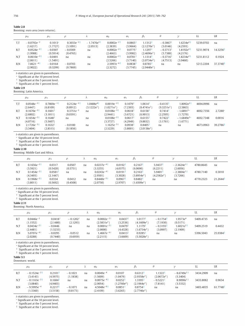
Table 3.1

Downturn: world.


B,T − 0.1524e−2‡ 0.2101‡ − 0.1021 na 0.0049e−4 0

(3.4143) (4.5975) (1.1838) (1.5609) (1

N,T − 0.1163e−2‡ 0.1684‡ na na 0.0075e−4‡ 0

(3.0840) (4.9403) (2.9054) (1

B,N − 9.5995e−4 0.2217‡ − 0.1071 na 4.5048e−6† 0

(1.5360) (3.5158) (0.8173) (2.4109) (3

t-statistics are given in parentheses.∗ Significant at the 10 percent level.† Significant at the 5 percent level.
‡ Significant at the 1 percent level.
α1 β1 θ γ LL LR

0.0865‡ 1.1312‡ − 0.3867‡ 1.6234e2‡ 5239.0702 na

(3.9664) (2.1270e1) (5.0146) (4.2593)

0.0775‡ 1.1297‡ − 0.3713‡ 1.8192e2‡ 5231.9074 14.3256‡

(3.9982) (2.4696e1) (5.7388) (4.2176)

0.0781‡ 1.1314‡ − 0.3716‡ 1.8234e2‡ 5231.8112 0.1924

(3.7140) (2.0734e2) (4.7513) (3.9460)

0.0838‡ 0.8785‡ na na 5213.2204 37.3740‡

(3.7745) (2.9440e1)

1 β1 θ γ LL LR

0.1079‡ 1.0614‡ − 0.4135‡ 1.8092e2‡ 4694.0996 na

7.2303) (8.4741e1) (9.3251e1) (2.5863)

0.0618‡ 0.6158‡ 0.7414† − 1.68912∗ 4692.7356 2.7280∗

3.6721) (6.9013) (2.2505) (1.7270)

0.0617‡ 0.6155‡ 0.7422‡ − 1.6849e2∗ 4692.7348 0.0016

4.2949) (9.8832) (3.1761) (1.6771)

0.0938‡ 0.8405‡ na na 4673.0963 39.2786‡

3.8001) (2.0138e1)

β1 θ γ LL LR

‡ 0.2167‡ 5.9437‡ − 2.3624e1‡ 4780.8645 na

) (6.0690) (6.2211) (2.6056)‡ 0.2163‡ 5.9401‡ − 2.3804e1‡ 4780.7140 0.3010

) (3.8954e1) (4.2582e1) (3.7266)‡ 0.8482‡ na na 4770.2323 21.2644‡

) (1.6509e1)

β1 θ γ LL LR

7‡ 1.0177‡ − 0.1754‡ 1.9573e4 5409.4735 na

36) (4.1609e1) (7.1930) (0.5171)

9‡ 1.1179‡ − 0.3193‡ 1.6021e2† 5409.2519 0.4432

28) (1.6734e1) (3.0997) (2.1909)

3‡ 0.9285‡ na na 5396.5043 25.9384‡

09) (5.5028e1)

β1 θ γ LL LR

0.6312‡ 1.1322‡ − 8.6749e1‡ 3434.2909 na

(2.9358e1) (2.0672e1) (5.3404)

1.3395‡ − 0.5221‡ 8.9090e1‡ 3433.8082 0.96542) (2.1964e1) (7.8141) (3.5332)

0.8754‡ na na 3403.4035 61.7748‡

(2.7746e1)


T

D

3∗

2

2

5†

T

D

3)−4∗

−4

−6†

T

D

α1

0.024

(2.580

0.084

(3.790

0.130

(4.073

T

D

α1

0.06

(5.61

0.07

(3.62

0.10

(4.33

T

D

α1

0.015

(2.755

0.058

(3.058

0.092

(4.298

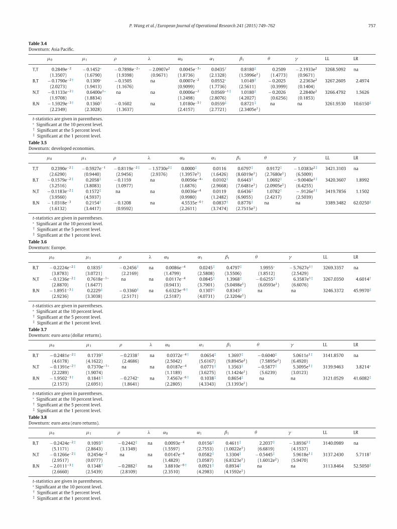
able 3.4

ownturn: Asia Pacific.

μ0 μ1 ρ λ α0

T,T 0.2849e−2 − 0.1452∗ − 0.7898e−2∗ − 2.0907e2 0.0045e−

(1.3507) (1.6790) (1.9398) (0.9671) (1.8736)

B,T − 0.1790e−2† 0.1309∗ − 0.1505 na 0.0007e−

(2.0273) (1.9413) (1.1676) (0.9099)

N,T − 0.1133e−2† 0.6400e1∗ na na 0.0006e−

(1.9708) (1.8834) (1.2498)

B,N − 1.5929e−3† 0.1360† − 0.1602 na 1.0180e−

(2.2349) (2.3028) (1.3637) (2.4157)


able 3.5

ownturn: developed economies.

μ0 μ1 ρ λ α0

T,T 0.2390e−2‡ − 0.5927e−1 − 0.8119e−2‡ − 1.5730e2‡ 0.0000‡

(2.6290) (0.9440) (2.9456) (2.9376) (1.3957e

B,T − 0.1579e−2‡ 0.2058‡ − 0.1159 na 0.0056e

(3.2516) (3.8083) (1.0977) (1.6876)

N,T − 0.1183e−2‡ 0.1572‡ na na 0.0036e

(3.9560) (4.5937) (0.9980)

B,N − 1.0318e−3 0.2154‡ − 0.1208 na 4.5535e

(1.6132) (3.4417) (0.9592) (2.2611)


able 3.6

ownturn: Europe.

μ0 μ1 ρ λ α0

B,T − 0.2224e−2‡ 0.1835‡ − 0.2456† na 0.0086e−4

(3.8783) (3.0721) (2.2169) (1.4799)

N,T − 0.1236e−2‡ 0.7618e−1∗ na na 0.0117e−4

(2.8870) (1.6477) (0.9413)

B,N − 1.8951−3‡ 0.2229‡ − 0.3360† na 6.6323e−6†

(2.9236) (3.3038) (2.5171) (2.5187)


able 3.7

ownturn: euro area (dollar returns).

μ0 μ1 ρ λ α0

B,T − 0.2481e−2‡ 0.1739‡ − 0.2338† na 0.0372e−4†

(4.6178) (4.1622) (2.4686) (2.5042)

N,T − 0.1391e−2† 0.7370e−1∗ na na 0.0187e−4

(2.2289) (1.9074) (1.1189)

B,N − 1.9502−3† 0.1841‡ − 0.2742∗ na 7.4567e−6†

(2.1573) (2.6951) (1.8641) (2.2805)


able 3.8

ownturn: euro area (euro returns).

μ0 μ1 ρ λ α0

B,T − 0.2424e−2‡ 0.1093‡ − 0.2442‡ na 0.0093e−4

(5.1171) (2.8643) (3.1349) (1.5597)

N,T − 0.1266e−2‡ 0.2454e−2 na na 0.0147e−4

(2.9517) (0.0777) (1.4829)

B,N − 2.0111−3‡ 0.1348† − 0.2882‡ na 3.8810e−6†

(2.6660) (2.5439) (2.8109) (2.3510)

α1 β1 θ γ LL LR

0.0435† 0.8180‡ 0.2509 − 2.1933e2 3268.5092 na

(2.1328) (1.5996e1) (1.4773) (0.9671)

0.0552∗ 1.0149† − 0.2025 2.2363e2 3267.2605 2.4974

(1.7736) (2.5611) (0.3999) (0.1404)

0.0569−1‡ 1.0180‡ − 0.2026 2.2840e2 3266.4792 1.5626

(2.8076) (4.2027) (0.6256) (0.1853)

0.0559‡ 0.8721‡ na na 3261.9530 10.6150‡

(2.7721) (2.3405e1)

α1 β1 θ γ LL LR

0.0116 0.6797‡ 0.9172‡ − 1.0383e2‡ 3421.3103 na

(1.6426) (8.6019e1) (2.7680e1) (6.5009)

0.0102‡ 0.6443‡ 1.0692‡ − 9.0040e1‡ 3420.3607 1.8992

(2.9668) (7.6481e1) (2.0905e1) (6.4255)

0.0119 0.6436‡ 1.0782† − .9126e1† 3419.7856 1.1502

(1.2482) (6.9055) (2.4217) (2.5039)

0.0837‡ 0.8776‡ na na 3389.3482 62.0250‡

(3.7474) (2.7515e1)

β1 θ γ LL LR

5‡ 0.4797‡ 1.9955∗ − 5.7627e1† 3269.3357 na

8) (3.5506) (1.8512) (2.5429)

5‡ 1.3968‡ − 0.6255‡ 6.3587e1‡ 3267.0350 4.6014†

1) (5.0498e1) (6.0593e1) (6.6076)

7‡ 0.8343‡ na na 3246.3372 45.9970‡

1) (2.3204e1)

β1 θ γ LL LR

54‡ 1.3697‡ − 0.6040‡ 5.0611e1‡ 3141.8570 na

67) (9.8945e2) (7.5895e2) (6.4920)

71‡ 1.3563‡ − 0.5877‡ 5.3095e1‡ 3139.9463 3.8214∗

75) (1.1424e1) (5.6239) (3.0123)

38‡ 0.8654‡ na na 3121.0529 41.6082‡

43) (3.1393e1)

β1 θ γ LL LR

6‡ 0.4611‡ 2.2037‡ − 3.89361‡ 3140.0989 na

3) (1.0022e1) (6.6819) (4.1537)

2‡ 1.3304‡ − 0.5445‡ 5.9618e1‡ 3137.2430 5.7118†

7) (6.8323e1) (1.6012e2) (5.9470)

1‡ 0.8934‡ na na 3113.8464 52.5050‡

3) (4.1592e1)


α1

0.044

(2.085

0.060

(3.570

0.078

(3.571

α1

0.0

(1.1

0.0

(1.2

0.1

(3.9

−3

−3

−2

−6

0.023

(2.786

0.002

(2.184

0.152

(2.582

α1

0.

(2.

0.

(0.

0.

(3.

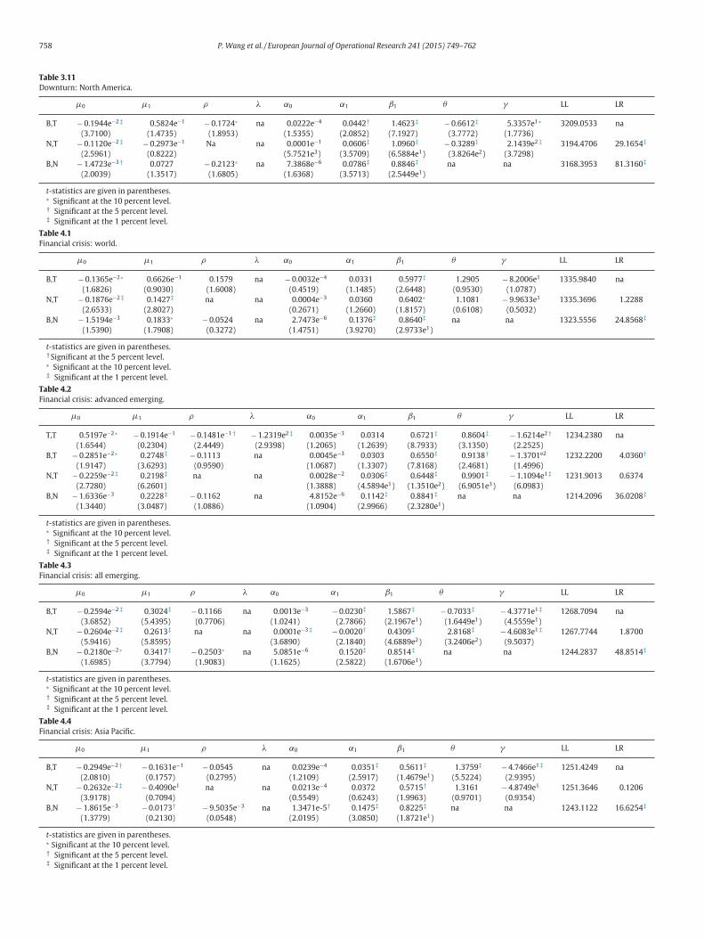
Table 3.11

Downturn: North America.

μ0 μ1 ρ λ α0

B,T − 0.1944e−2‡ 0.5824e−1 − 0.1724∗ na 0.0222e−4

(3.7100) (1.4735) (1.8953) (1.5355)

N,T − 0.1120e−2‡ − 0.2973e−1 Na na 0.0001e−1

(2.5961) (0.8222) (5.7521e3)

B,N − 1.4723e−3† 0.0727 − 0.2123∗ na 7.3868e−6

(2.0039) (1.3517) (1.6805) (1.6368)


Table 4.1

Financial crisis: world.

μ0 μ1 ρ λ α0

B,T − 0.1365e−2∗ 0.6626e−1 0.1579 na − 0.0032e−4

(1.6826) (0.9030) (1.6008) (0.4519)

N,T − 0.1876e−2‡ 0.1427‡ na na 0.0004e−3

(2.6533) (2.8027) (0.2671)

B,N − 1.5194e−3 0.1833∗ − 0.0524 na 2.7473e−6

(1.5390) (1.7908) (0.3272) (1.4751)

t-statistics are given in parentheses.†Significant at the 5 percent level.∗ Significant at the 10 percent level.‡ Significant at the 1 percent level.

Table 4.2

Financial crisis: advanced emerging.

μ0 μ1 ρ λ α0

T,T 0.5197e−2∗ − 0.1914e−1 − 0.1481e−1† − 1.2319e2‡ 0.0035e

(1.6544) (0.2304) (2.4449) (2.9398) (1.2065)

B,T − 0.2851e−2∗ 0.2748‡ − 0.1113 na 0.0045e

(1.9147) (3.6293) (0.9590) (1.0687)

N,T − 0.2259e−2‡ 0.2198‡ na na 0.0028e

(2.7280) (6.2601) (1.3888)

B,N − 1.6336e−3 0.2228‡ − 0.1162 na 4.8152e

(1.3440) (3.0487) (1.0886) (1.0904)


Table 4.3

Financial crisis: all emerging.


B,T − 0.2594e−2‡ 0.3024‡ − 0.1166 na 0.0013e−3 −(3.6852) (5.4395) (0.7706) (1.0241)

N,T − 0.2604e−2‡ 0.2613‡ na na 0.0001e−3‡ −(5.9416) (5.8595) (3.6890)

B,N − 0.2180e−2∗ 0.3417‡ − 0.2503∗ na 5.0851e−6

(1.6985) (3.7794) (1.9083) (1.1625)


Table 4.4

Financial crisis: Asia Pacific.

μ0 μ1 ρ λ α0

B,T − 0.2949e−2† − 0.1631e−1 − 0.0545 na 0.0239e−4

(2.0810) (0.1757) (0.2795) (1.2109)

N,T − 0.2632e−2‡ − 0.4090e1 na na 0.0213e−4

(3.9178) (0.7094) (0.5549)

B,N − 1.8615e−3 − 0.0173† − 9.5035e−3 na 1.3471e-5†

(1.3779) (0.2130) (0.0548) (2.0195)


β1 θ γ LL LR

2† 1.4623‡ − 0.6612‡ 5.3357e1∗ 3209.0533 na

2) (7.1927) (3.7772) (1.7736)

6‡ 1.0960‡ − 0.3289‡ 2.1439e2‡ 3194.4706 29.1654‡

9) (6.5884e1) (3.8264e2) (3.7298)

6‡ 0.8846‡ na na 3168.3953 81.3160‡

3) (2.5449e1)

β1 θ γ LL LR

331 0.5977‡ 1.2905 − 8.2006e1 1335.9840 na

485) (2.6448) (0.9530) (1.0787)

360 0.6402∗ 1.1081 − 9.9633e1 1335.3696 1.2288

660) (1.8157) (0.6108) (0.5032)

376‡ 0.8640‡ na na 1323.5556 24.8568‡

270) (2.9733e1)

α1 β1 θ γ LL LR

0.0314 0.6721‡ 0.8604‡ − 1.6214e2† 1234.2380 na

(1.2639) (8.7933) (3.1350) (2.2525)

0.0303 0.6550‡ 0.9138† − 1.3701e2 1232.2200 4.0360†

(1.3307) (7.8168) (2.4681) (1.4996)

0.0306‡ 0.6448‡ 0.9901‡ − 1.1094e1‡ 1231.9013 0.6374

(4.5894e1) (1.3510e2) (6.9051e3) (6.0983)

0.1142‡ 0.8841‡ na na 1214.2096 36.0208‡

(2.9966) (2.3280e1)

β1 θ γ LL LR

0‡ 1.5867‡ − 0.7033‡ − 4.3771e1‡ 1268.7094 na

6) (2.1967e1) (1.6449e1) (4.5559e1)

0† 0.4309‡ 2.8168‡ − 4.6083e1‡ 1267.7744 1.8700

0) (4.6889e2) (3.2406e2) (9.5037)

0‡ 0.8514‡ na na 1244.2837 48.8514‡

2) (1.6706e1)

β1 θ γ LL LR

0351‡ 0.5611‡ 1.3759‡ − 4.7466e1‡ 1251.4249 na

5917) (1.4679e1) (5.5224) (2.9395)

0372 0.5715† 1.3161 − 4.8749e1 1251.3646 0.1206

6243) (1.9963) (0.9701) (0.9354)

1475‡ 0.8225‡ na na 1243.1122 16.6254‡

0850) (1.8721e1)


T

F

α1

0.0

(1.7

0.0

(1.2

0.1

(3.6

T

F

α1

− 0.0

(3.5

− 0.0

(3.3

0.1

(3.1

T

F

α1

−(

−(

−(

(

T

F

−3∗

−3

−3

−6

T

F

1

0.608

(1.498

0.853

(1.216

0.127

(2.988

able 4.5

inancial crisis: developed economies.

μ0 μ1 ρ λ α0

B,T − 0.1385e−2∗ 0.3717e−1 0.1424 na − 0.0023e−4

(1.8491) (0.3830) (1.0112) (0.3016)

N,T − 0.1872e−2‡ 0.1030† na na 0.0004e−3

(3.0348) (2.3666) (0.3741)

B,N − 1.6851e−3∗ 0.1568 − 0.0806 na 2.8463e−6

(1.6640) (1.5624) (1.4815) (1.3451)


able 4.6

inancial crisis: Europe.

μ0 μ1 ρ λ α0

B,T − 0.1562e−2‡ − 0.3714e−1 − 0.0237e−2 na 0.0001e−5‡

(5.1302) (1.4034) (0.0037) (8.2581e1)

N,T − 0.2370e−2‡ − 0.7614e−2 na na 0.0001e−4

(1.3514e2) (0.1780) (0.0480)

B,N − 1.4959e−3 − 0.0356 − 0.0696† na 5.3647e−6∗

(1.4277) (0.4751) (0.4476) (1.7553)


able 4.7

inancial crisis: euro area (dollar returns).

μ0 μ1 ρ λ α0

T,T − 0.3862e−2‡ 0.7832e−1† 0.3621e−2‡ 5.2104e2‡ 0.0001e−6

(3.2971e1) (2.0229) (4.4492) (1.2202e1) (0.8251)

B,T − 0.2326e−2‡ − 0.5703e−1† 0.3714e−1‡ na 0.0025e−4

(1.3136e1) (2.2340) (2.8273) (0.6978)

N,T − 0.2161e−2‡ − 0.1180e−1 na na 0.0001e−6

(7.0497e1) (0.2022) (1.5455)

B,N − 1.1169e−3 − 0.0520 − 0.0355 na 5.4533e−6

(1.1784) (0.7071) (0.2431) (1.3201)


able 4.8

inancial crisis: euro area (euro returns).

μ0 μ1 ρ λ α0

T,T 0.2298e−2 − 0.1879‡ − 0.9287e−2† − 8.6825e1∗ 0.0034e

(1.4694) (3.4195) (2.3837) (1.7343) (1.7968)

B,T − 0.2597e−2† − 0.2241e−1 − 0.5964e−1 na 0.0037e

(2.5262) (0.3469) (0.4693) (1.5021)

N,T − 0.2302e−2‡ − 0.5062e−1 na na 0.0032e

(2.7148) (1.0978) (1.4308)

B,N − 1.7547e−3 − 0.0398 − 0.1396 na 9.1045e

(1.5671) (0.5501) (0.8387) (1.3769)


able 4.9

inancial crisis: Latin America.


B,T − 0.0444e−2† 0.8625e−2 0.2774e−2 na 0.0001e−6‡ −(8.6968) (0.2269) (0.4053) (5.7606e1)

N,T − 0.1261e−2‡ 0.1439e−1 na na 0.0001e−2‡ −(1.4802e3) (0.3247) (2.0529e3)

B,N − 0.2386e−2 0.1109 − 0.2319 na 0.1555e−4

(1.1976) (1.3245) (1.4467) (1.4263)

β1 θ γ LL LR

344∗ 0.5929‡ 1.2892 − 7.3749e1 1330.3329 na

316) (3.5843) (1.4122) (1.4077)

375 0.6273† 1.0678 − 8.4808e1 1329.8940 0.8778

724) (2.3708) (0.7779) (0.8430)

295‡ 0.8706‡ na na 1319.0668 22.5322‡

551) (2.8370e1)

β1 θ γ LL LR

074‡ 0.6997‡ 0.9473‡ − 1.2143e1‡ 1241.6320 na

005) (2.6024e2) (6.4246e2) (1.0364e1)

054‡ 0.5457‡ 1.8328‡ − 6.8313e1‡ 1241.0638 1.1364

635) (1.4112e2) (7.2091e1) (1.3710e1)

646‡ 0.8460‡ na na 1213.7000 55.8640‡

864) (2.3829e1)

β1 θ γ LL LR

0.6728e−2‡ 0.5837‡ 1.5574‡ − 7.2479e1‡ 1231.6824 na

2.8267) (1.8460e2) (1.3264e2) (7.9288)

0.8951e−2‡ 0.6708‡ 1.1114‡ − 8.9763e1‡ 1231.2429 0.8790

6.0001) (5.2147e2) (1.1106e2) (5.6701e1)

0.3872e−2‡ 0.5882‡ 1.5240‡ − 7.1421e1‡ 1230.6768 1.1322

2.3132e1) (1.5344e2) (2.4688e2) (3.3506)

0.1737‡ 0.8396‡ na na 1206.8667 48.7524‡

2.8420) (1.9552e1)

α1 β1 θ γ LL LR

0.0339‡ 0.6654‡ 0.8889‡ − 1.3294e2† 1259.7191 na

(5.2401) (6.6267e2) (5.9016e1) (2.4280)

0.0338† 0.6518‡ 0.9325∗ − 1.2004e2 1259.4718 0.4946

(2.3623) (5.3479) (1.7382) (1.2516)

0.0352‡ 0.6513‡ 0.9421∗ 1.1716e2 1259.3789 0.1858

(2.8203) (6.2624) (1.9204) (1.6226)

0.1430‡ 0.8490‡ na na 1239.8737 39.1962‡

(2.7192) (1.8874e1)

β1 θ γ LL LR

8e−2‡ 0.4122‡ 2.9728‡ − 2.2762e1‡ 1119.1785 na

4e2) (1.9631e2) (1.1861e3) (1.4573e1)

1e−2‡ 0.5071‡ 2.0596‡ − 2.7199e1‡ 1118.4207 1.5156

9e3) (4.5097) (1.2567e4) (1.0387e2)

9‡ 0.8628‡ na na 1098.3477 41.6616‡

3) (1.9895e1)


0.130

0.125

0.933

0.357

0.109

3.974

α1

0.02

(1.49

0.02

(1.47

0.11

(4.19

α1

0.131

(4.462

0.128

(4.098

0.200

(4.381

α1

0.

(3.

0.

(1.

0.

(1.

0.

(3.

a

m

s

p

s

1

s

λr

Table 4.10

Financial crisis: Middle East and Africa.


B,T − 0.2271e−2‡ 0.4932e−1 0.1652e−1 na 0.0014e−4

(4.6149) (0.7105) (0.2288) (0.4202) (

N,T − 0.2773e−2† 0.8043e−1 na na 0.0031e−4 −(2.2980) (1.1767) (0.1815) (

B,N − 0.8867e−3 0.0600 0.0323 na 6.2909e−6

(0.6102) (0.6285) (0.2246) (1.6227) (


Table 4.11

Financial crisis: North America.

μ0 μ1 ρ λ α0

B,T − 0.1896e−2∗ − 0.1518∗ − 0.4714e−1 na 0.0011e−3

(1.8911) (1.7173) (0.3940) (0.7522)

N,T − 0.1656e−2† − 0.1771‡ na na 0.0079e−4

(2.4247) (3.2112) (0.7920)

B,N − 0.1958e−2† − 0.1061 − 0.1408 na 0.4632e−5

(1.9697) (1.2871) (1.1328) (1.3716)


Table 5.9

Stock market stagnation: Latin America.

μ0 μ1 ρ λ α0

B,T 0.6692e−3 0.1674‡ 0.1520† na 0.0187e−3‡

(1.1680) (3.6298) (1.9856) (3.7049)

N,T − 0.0463e−3 0.2379‡ na na 0.0197e−3‡

(0.1043) (9.8736) (3.6377)

B,N 0.1453e−2† 0.1682‡ 0.1170 na 0.2288e−4‡

(2.3391) (3.6455) (1.3413) (3.1122)


Table 5.10

Stock market stagnation: Middle East and Africa.

μ0 μ1 ρ λ α0

T,T 0.1242e−4‡ 0.8877e−1‡ − 0.1858e−2‡ − 8.5631e3‡ 0.0013e−2∗

(6.1201) (4.6855) (4.8660) (6.4917) (1.7358)

B,T 0.2482e−3 0.1560‡ 0.1338e−1 na 0.0022e−4

(0.5905) (3.3372) (0.1489) (0.8387)

N,T 0.2220e−3 0.1588‡ na na 0.0169e−4

(0.8072) (6.1770) (0.6570)

B,N 0.3111e−3 0.1948‡ − 0.1169 na 1.0059e−5∗

(0.6764) (4.5224) (1.4945) (1.6878)


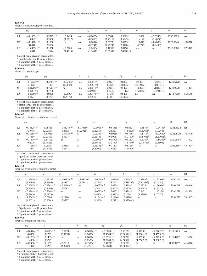
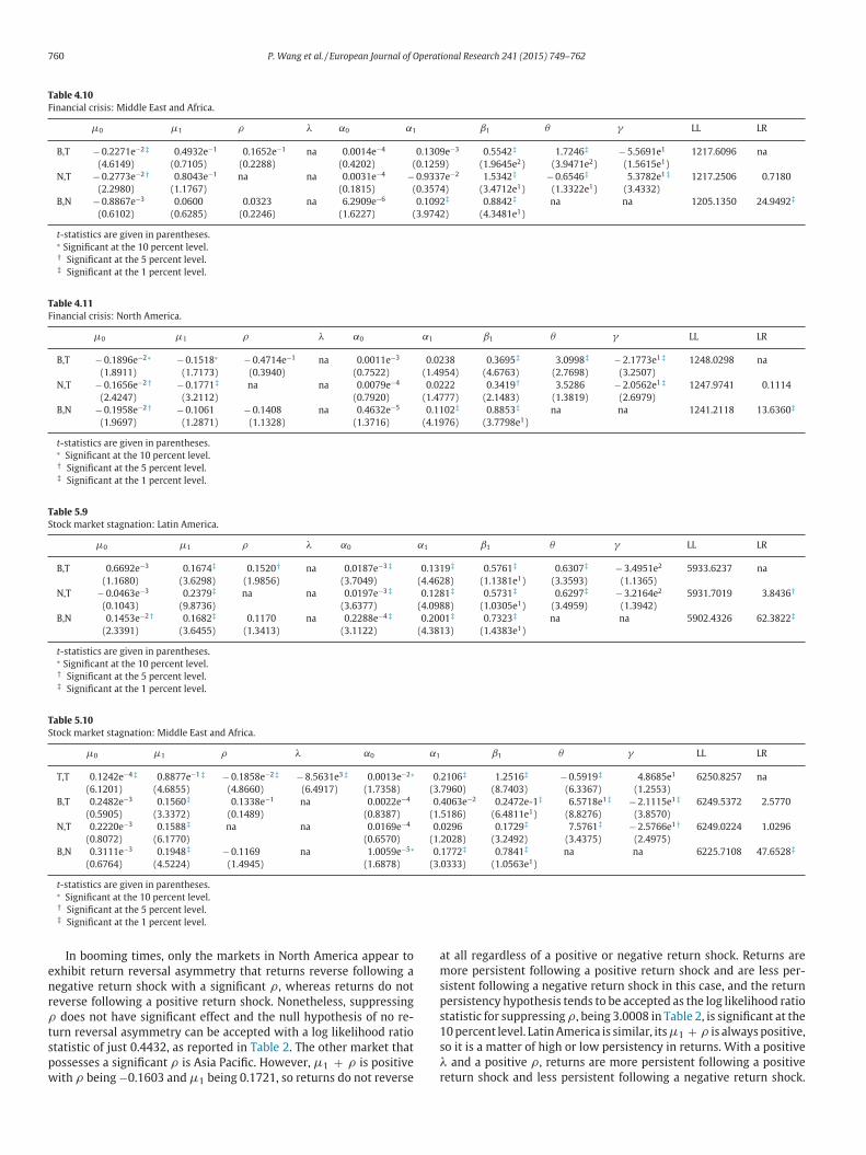
In booming times, only the markets in North America appear to

exhibit return reversal asymmetry that returns reverse following a

negative return shock with a significant ρ , whereas returns do not

reverse following a positive return shock. Nonetheless, suppressing

ρ does not have significant effect and the null hypothesis of no re-

turn reversal asymmetry can be accepted with a log likelihood ratio

statistic of just 0.4432, as reported in Table 2. The other market that

possesses a significant ρ is Asia Pacific. However, μ1 + ρ is positive

with ρ being −0.1603 and μ1 being 0.1721, so returns do not reverse

β1 θ γ LL LR

9e−3 0.5542‡ 1.7246‡ − 5.5691e1 1217.6096 na

9) (1.9645e2) (3.9471e2) (1.5615e1)

7e−2 1.5342‡ − 0.6546‡ 5.3782e1‡ 1217.2506 0.7180

4) (3.4712e1) (1.3322e1) (3.4332)

2‡ 0.8842‡ na na 1205.1350 24.9492‡

2) (4.3481e1)

β1 θ γ LL LR

38 0.3695‡ 3.0998‡ − 2.1773e1‡ 1248.0298 na

54) (4.6763) (2.7698) (3.2507)

22 0.3419† 3.5286 − 2.0562e1‡ 1247.9741 0.1114

77) (2.1483) (1.3819) (2.6979)

02‡ 0.8853‡ na na 1241.2118 13.6360‡

76) (3.7798e1)

β1 θ γ LL LR

9‡ 0.5761‡ 0.6307‡ − 3.4951e2 5933.6237 na

8) (1.1381e1) (3.3593) (1.1365)

1‡ 0.5731‡ 0.6297‡ − 3.2164e2 5931.7019 3.8436†

8) (1.0305e1) (3.4959) (1.3942)

1‡ 0.7323‡ na na 5902.4326 62.3822‡

3) (1.4383e1)

β1 θ γ LL LR

2106‡ 1.2516‡ − 0.5919‡ 4.8685e1 6250.8257 na

7960) (8.7403) (6.3367) (1.2553)

4063e−2 0.2472e-1‡ 6.5718e1‡ − 2.1115e1‡ 6249.5372 2.5770

5186) (6.4811e1) (8.8276) (3.8570)

0296 0.1729‡ 7.5761‡ − 2.5766e1† 6249.0224 1.0296

2028) (3.2492) (3.4375) (2.4975)

1772‡ 0.7841‡ na na 6225.7108 47.6528‡

0333) (1.0563e1)

t all regardless of a positive or negative return shock. Returns are

ore persistent following a positive return shock and are less per-

istent following a negative return shock in this case, and the return

ersistency hypothesis tends to be accepted as the log likelihood ratio

tatistic for suppressing ρ , being 3.0008 in Table 2, is significant at the

0 percent level. Latin America is similar, itsμ1 + ρ is always positive,

o it is a matter of high or low persistency in returns. With a positive

and a positive ρ , returns are more persistent following a positive

eturn shock and less persistent following a negative return shock.


T

A

a

ρd

a

t

D

a

n

t

P

t

F

A

T

r

o

i

w

e

p

d

s

t

N

–

B

a

t

i

s

e

a

i

i

t

s

T

r

p

t

h

e

l

f

c

s

p

r

c

f

C

t

f

s

t

c

b

o

(

e

a

p

i

a

μT

s

b

a

o

s

t

a

b

t

o

W

h

c

s

f

a

o

n

s

s

t

n

p

i

i

a

H

s

s

s

s

s

e

k

a

o

t

p

t

p

t

n

s

N

d

i

f

d

s

f

t

o

n

a

s

v

1

m

he return persistency hypothesis also tends to be accepted for Latin

merica with a log likelihood ratio statistic of 2.7280, being significant

t the 10 percent level. In the case of euro area (euro returns), although

(0.3033e−2) is significant, it is less than 1/30th of μ1 (0.1013), so it

oes not have a non-negligible effect on return persistency.

Inspecting the results, it can be observed that return reversal

symmetry is confined to the developed world in economic down-

urns. In this category are Europe, the euro area and North America.

eveloped markets as a whole exhibit a pattern of return reversal

symmetry, albeit by a very small scale, so does Asia Pacific, domi-

ated by the Japanese market. With a ρ of −0.7898e−2 that is less

han 1/10th of −0.1452 for μ1 in absolute value in the case of Asia

acific as reported in Table 3, this return reversal asymmetry is prac-

ically immaterial, taking any minimal transaction costs into account.

or developed markets, return reversal asymmetry is as trivial as in

sia Pacific, with its ρ being less than 1/7th of μ1 in absolute value.

he full specification of a smooth transition function for both mean

eversion/persistence asymmetry and variance asymmetry works for

nly two of the return series, developed markets and Asia Pacific, and

t does not perform better than the B,T specification statistically, with

hich return reversal asymmetry does not show up. For Europe, the

uro area and North America, the best specification is B,T, and sup-

ressing the mean reversion parameter ρ for the N,T specification re-

uces log likelihood function values. The log likelihood ratio statistic is

ignificant at the 10 percent level for euro area (dollar returns) and at

he 5 percent level for Europe and euro area (euro returns). Above all,

orth America demonstrates the strongest return reversal asymmetry

the log likelihood ratio statistic for the N,T specification vis-à-vis the

,T specification, at 29.1654, is highly significant at the 1 percent level.

In severe economic downturns, returns simply remain negative

nd there is no tendency to reverse, leave it alone asymmetry in re-

urn reversals. This is evident by a significant intercept and insignif-

cant slope parameter in most of the cases with the preferred model

pecifications, reported for the financial crisis period in Table 4. An

xception is advanced emerging markets where returns do reverse to

significant degree not only statistically but also practically mean-

ngfully. Its return reversal asymmetry parameter ρ , at −0.1481e−1,

s greater than the intercept μ0 of 0.5197e−2 in absolute value. Addi-

ionally the T,T specification, with which return reversal asymmetry

hows up, cannot be rejected for the alternative of a B,T specification.

he result suggests that investors in advanced emerging markets are

elatively optimistic, expecting a negative return to reverse to become

ositive following a negative return shock, which is inconceivable in

he developed economy in that period. Indeed, the developing world

as suffered much less than the developed American and European

conomies in the last financial crisis. In the case of euro area (dol-

ar returns and euro returns), although the T,T specification works

or them with a statistically significant ρ and a statistically signifi-

ant λ, the absolute value of ρ is 1/20th of the absolute value of the

lope parameter μ1 in both cases. Such return reversal asymmetry is

ractically immaterial, misleading and illusionary. Indeed, imposing

estrictions on the return reversal asymmetry parameters can be ac-

epted, with a very insignificant log likelihood ratio statistic of 0.8790

or euro area (dollar returns) and 0.4946 for euro area (euro returns).

onsequently, the T,T specification is not superior to the B,T specifica-

ion, with which an opposite return reversal asymmetry is produced

or the former that returns reverse faster following a positive return

hock and no asymmetry in return reversals for the latter. An addi-

ional remark on this period is that econometric estimation is also in

risis, sometimes with peculiar t-statistics though the algorithm has

een managed to converge, albeit involving a kind of fine-tuning. α1

r α0 is negative in some cases but the stationarity condition of Eq.

10) is still met nonetheless.

No return reversal asymmetry is found in stock market stagnation

ither. Viewing Table 5, returns are more persistent following a neg-

tive return shock for Latin America. Suppressing ρ makes the model

erformance worse with a log likelihood ratio statistics of 3.8436 that

s significant at the 5 percent level. Therefore, such return persistency

symmetry does exist. Moreover, the size of ρ is in the same range of

1, which has practical implications. For Middle East and Africa, the

,T specification seems to work with a statistically significant ρ and a

tatistically significant λ. However, μ1 + ρ is always positive with ρeing −0.1858e−2 and μ1 being 0.8877e−1, so returns do not reverse

t all in any circumstance. The absolute value of ρ is about 1/50th

f the absolute value of the slope parameter μ1. Such statistically

ignificant figures are not only irrelevant but also misleading prac-

ically. With imposed restrictions being accepted, no return reversal

symmetry exists actually.

The T,T specification that adopts a smooth transition function for

oth return reversal/persistency asymmetry and volatility asymme-

ry is overwhelmingly disallowed, either due to non-convergence

f the algorithm or unfittingly lower log likelihood function values.

hen it has worked for a limited number of cases, the log likeli-

ood statistic for imposing restrictions is mostly insignificant, indi-

ating it is not superior to the B,T specification where return rever-

al/persistency asymmetry is modeled with a binary process. There-

ore, H1 that hypothesizes return reversal/persistency asymmetry is

quantitative response to previous return shocks, is rejected in favor

f a qualitative response.

Return reversal asymmetry is ambiguous. In most instances, ρ is

egative but insignificant. In limited cases where ρ is statistically

ignificant, it is much smaller than the slope parameter μ1 in ab-

olute value and is practically immaterial. Further and in booming

imes, suppressing the return reversal asymmetry parameter does

ot reduce the function value statistically but suppressing the return

ersistency asymmetry parameter does reduce the function value

n three out of 11 return indexes. That return reversal asymmetry

s ambiguous is upheld overwhelmingly, but that return persistency

symmetry is upheld to a lesser extent in stock market booms. i.e.,

5 is accepted overwhelmingly when stock returns experience rever-

als but is accepted to a lesser extent when stock returns persist. The

ituation is the same in stock market stagnation that return rever-

al asymmetry is ambiguous but return persistency asymmetry does

eem to exist. In severe stock market downturns or the financial crisis,

tock returns simply remain negative with no signs of reversals at all,

xcept one out of 11 cases; only returns on advance emerging mar-

et still reverse under such economic circumstance. Return reversal

symmetry is found to be primarily a developed market phenomenon

nly during market downturns.

Return reversal/persistency asymmetry is illusionary. Suppressing

he volatility asymmetry parameter incorrectly deteriorates model

erformance in all 31 cases, with a highly significant LR statistic for

he B,N specification reported in these 31 tables. More seriously, sup-

ressing the volatility asymmetry parameter induces asymmetric re-

urn revision/persistence in the mean equation. It has created a sig-

ificant ρ in six cases and produced a ρ showing some asymmetry

ymptom (negative with t > 1) in additional eight cases, from the

,T specification to the B,N specification. H6a is therefore accepted

ecisively. Adopting an over sophisticated T,T specification does not

mprove on model performance. This specification has only worked

or nine out of 31 cases. In seven of them, both ρ and λ are significantly

ifferent from zero. In one case, ρ is significantly negative but λ is in-

ignificant, which effectively becomes a binary threshold specification

or return reversal/persistency asymmetry. Seven out of nine cases,

his sophisticated specification is not superior to a binary thresh-

ld specification for return reversal/persistency asymmetry; it is also

ot superior to the specification without return reversal/persistency

symmetry. Among the only three cases where the sophisticated T,T

pecification achieves a statistically higher log likelihood function

alue than other specifications, one is at a lower significance level of

0 percent modest for a booming Latin America and the other at a

odest significance level of 5 percent for advance emerging market


p

l

a

r

w

i

R

A

B

C

D

D

H

H

I

K

K

K

M

N

N

N

P

W

Z

Z

in the financial crisis. With an absolute value of ρ being less than

1/30th of the absolute value of the slope parameter μ1 for a boom-

ing Latin America, this kind of asymmetry is immaterial. In only one

case this sophisticated specification is highly significantly superior

for the euro area (euro returns) in booming. Again, the absolute value

of ρ is less than 1/30th of the absolute value of the slope parameter

μ1. Therefore, even if this sophisticated T,T specification is superior

statistically in this case, its return reversal/persistency asymmetry

is practically immaterial and illusionary financially. As such, H6b is

upheld overwhelmingly.

The above analysis that examines the interactions between asym-

metries in mean reversion/persistence and in time-varying volatil-

ities reveals that return reversal/persistency asymmetry is illusion-

ary created by suppressing the volatility asymmetry parameter in-

correctly and by adopting over sophisticated model specifications.

On the other hand, return reversal asymmetry is found to be am-

biguous. The implications are that attempts to predict returns based

on return reversal/persistency asymmetry parameter values would

end up achieving no overall improvements when return rever-

sal/persistency asymmetry is ambiguous. Under this circumstance,

uncertainties in asymmetry in mean reversion/persistence are best

left for the variance asymmetry parameter to pick up. The attempts

will not help at all when return reversal/persistency asymmetry is

illusionary.

5. Conclusion

In this paper the protocol of return reversals and asymmetry in

return reversals that have prevailed in the empirical literature in the

last decade has been questioned. Return persistency and conceivably

asymmetry in return persistency have been proposed instead as an

alternative proposition in the study of asymmetries in stock markets,

which has been confirmed to be a more relevant but still uncon-

vincing paradigm. Then return reversal/persistency asymmetry and

volatility asymmetry have been jointly examined under various stock

market conditions. It has been found that return reversal asymme-

try is confined to developed markets only and during stock market

downtowns only. Return reversal asymmetry, while appears to show

up in limited cases under other market conditions including stock

market booms, stagnation and financial crises, is mostly ambiguous

and in fact illusionary. Overwhelmingly, suppressing the return re-

versal asymmetry parameter does not make a difference in model

erformance. Such ambiguity in return reversal asymmetry is best

eft with volatility asymmetry and picked up by modeling volatility

symmetry instead. Whereas return persistency and asymmetry in

eturn persistency are relatively more prevalent, though they are also

eak and cannot be confirmed resolutely for the majority of return

ndexes.

eferences

tkins, A. B., & Dyl, E. A. (1990). Price reversals, bid-ask spreads, and market efficiency.Journal of Financial and Quantitative Analysis, 25(4), 535–547.

remer, M., & Sweeney, R. J. (1991). The reversal of large stock-price decreases. Journal

of Finance, 46(2), 747–754.harles, A. (2010). The day-of-the-week effects on the volatility: The role of the asym-

metry. European Journal of Operational Research, 202(1), 143–152.e Bondt, W. F. M., & Thaler, R. (1985). Does the stock market overreact?. Journal of

Finance, 40(3), 793–805.issanaike, G. (1996). Are stock price reversals really asymmetric? A note. Journal of

Banking and Finance, 20(1), 189–201.ua, Z. S., & Zhang, B. (2008). Improving density forecast by modeling asymmetric fea-

tures: An application to S&P500 returns. European Journal of Operational Research,

185(2), 716–725.wang, S., & Rubesam, A. (2013). A behavioral explanation of the value anomaly based

on time-varying return reversals. Journal of Banking & Finance, 37(7), 2367–2377.ihara, Y., Kato, H. K., & Tokunaga, T. (2004). The winner–loser effect in Japanese stock

returns. Japan and the World Economy, 16(4), 471–485.edar-Levy, H., Yu, X., Kamesaka, A., & Ben-Zion, U. (2010). The impact of daily return

limit and segmented clientele on stock returns in China. International Review of

Financial Analysis, 19(4), 223–236.im, C. J., & Nelson, C. R. (1998). Testing for mean reversion in heteroskedastic data II:

Autoregression tests based on Gibbs sampling-augmented randomization. Journalof Empirical Finance, 5(4), 385–396.

outmos, G. (1998). Asymmetries in the conditional mean and the conditional vari-ance: Evidence from nine stock markets. Journal of Economics and Business, 50(3),

277–290.

alliaropulos, D., & Priestley, R. (1999). Mean reversion in Southeast Asian stock mar-kets. Journal of Empirical Finance, 6(4), 355–384.

am, K., Pyun, C. S., & Avard, S. L. (2001). Asymmetric reverting behavior of short-horizon stock returns: Evidence of stock market overreaction. Journal of Banking

and Finance, 25(4), 807–824.am, K., Pyun, C. S., & Avard, S. L. (2002). Asymmetric mean-reversion and contrarian

profits: ANST-GARCH approach. Journal of Empirical Finance, 9(5), 563–588.

elson, D. B. (1991). Conditional heteroskedasticity in asset returns: A new approach.Econometrica, 59(2), 347–370.

ark, B. J. (2011). Asymmetric herding as a source of asymmetric return volatility.Journal of Banking & Finance, 35(10), 2657–2665.

ang, P., & Wang, P. J. (2011). Asymmetry in return reversals or asymmetry in volatil-ities?. Quantitative Finance, 11(2), 271–285.

arowin, P. (1989). Short-run market overreaction: Size and seasonality effects. Journal

of Portfolio Management, 15(3), 26–29.arowin, P. (1990). Size, seasonality, and stock market overreaction. Journal of Financial

and Quantitative Analysis, 25(1), 113–125.

http://refhub.elsevier.com/S0377-2217(14)00768-1/bib0001



































http://refhub.elsevier.com/S0377-2217(14)00768-1/bib0017a






http://refhub.elsevier.com/S0377-2217(14)00768-1/bib0017b


























asymmetries in stock markets

Documents