Analogy PrincipleAsymptotic Theory — Part II

James J. HeckmanUniversity of Chicago

Econ 312This draft, April 5, 2006

Consider four methods:

1. Maximum Likelihood Estimation (MLE)

2. (Nonlinear) Least Squares

3. Methods of Moments

4. Generalized Method of Moments (GMM)

These methods are not always distinct for a particular problem.Consider the classical normal linear regression model:

= +

1

Under standard assumptions

1. (0 2); i.i.d.;

2. non-stochastic; and

3. 0 full rank.

OLS is all four rolled into one.

In this lecture we will show how one basic principle – theAnalogy Principle –underlies all of these modern econometricmethods.

2

1 Analogy Principle: The Large Sam-ple Version

This is originally due to Karl Pearson or Goldberger.

The intuition behind the analogy principle is as follows:

‘Suppose we know some properties that are satisfied for the“true parameter" in the population. If we can find a para-meter value in the sample that causes the sample to mimicthe properties of the population, we might use this parametervalue to estimate the true parameter.’

3

The main points of this principle are set out in §1.1. Theconditions for consistency of the estimator are discussed in§1.2. In §1.3, an abstract example with a finite parameter setillustrates the application of the analog principle and the role ofregularity conditions in ensuring consistency of the estimator.

4

1.1 Outline of the Analog Principle

The ideas constituting the analog principle can be groupedunder four steps:

1. The model. Suppose there exists a ‘true model’ in thepopulation – ( 0) = 0 – an implicit equation.0 is a true parameter vector, and the model is definedfor other values (at least some other) of .

2. Criterion function. Based on the model, construct a ‘cri-terion function’ of model and data:

( )

which has property in the population when = 0 (the‘true’ parameter vector).

5

3. Analog in sample. In the sample, construct an ‘analog’to , ( ), which has the following properties:

(a) ( ) ( )a. s. unif.

( ),where is the sample size; and

(b) ( )mimics in sample properties of ( )1

in the population.

4. The estimator. Let ˆ be the estimator of 0 in sampleformed from the analog in sample, which causes sample(.) to have the property .

1Hereafter, we shall suppress the dependence of the criterion functionand the sample analog on the data ( ) for notational conve-

nience.

6

1.2 Consistency and Regularity

Definition 1 (Consistency) We say that an estimator ˆ isa consistent estimator of parameter 0 if

ˆ 0.

In general, to prove that the estimator formed using the analogprinciple ˆ is consistent, we need to make the following twoassumptions, which are referred to as the regularity conditions:

1. Identification condition. Generally this states that only0 causes to possess property , at least in some neigh-borhood of 0; i.e. 0 must be at least locally identified.

7

2. Uniform convergence of the analog function. We need thesample analog (ˆ ) to converge ‘nicely’. In particular,we need the convergence of the sample analog criterionfunction to the criterion function – ( ) ( )( ) – to be uniform.

8

The first condition ensures that 0 can be identified. If thereis more than one value of that causes to have property ,then we cannot be sure that only one value of will causeto assume property in the sample. In this case we may notbe able to determine what ˆ estimates.

The second condition is a technical one that ensures that ifhas a property such as continuity or di erentiability, this

property is inherited by .

Specific proofs of consistency depend on which property wesuppose has when = 0.

9

1.3 An Abstract Example

The intuition underlying the analog principle method and therole of the regularity conditions is illustrated in the simple(non-stochastic) example below.

• Assume an abstract model ( 0) which leads to acriterion function ( ) which has the property

:= ( ) is maximized at = 0 (in population).

• Construct a sample analog of the criterion functionsuch that

( ) ( ) .

10

• Select ˆ to maximize ( ) for each . Then, if con-vergence is ‘OK’ (we get that under the regularity con-ditions), we have convergence in the sample to the max-imizer in the population; i.e. we have ˆ as .

11

Now suppose = {1 2 3} is a finite set, so that ˆ assumesonly one of three values. Then under regularity condition 1(q.v. §1.2), ( ) is maximized at one of these.Further, by construction we have¡

= {1 2 3}¢ ( ) ( ).

Note that the rule picks

ˆ = argmax ( ).

This estimator must work well (i.e. be consistent for for ‘bigenough’ , because for each . Why? We looselysketch a proof of the consistency of ˆ for below.

12

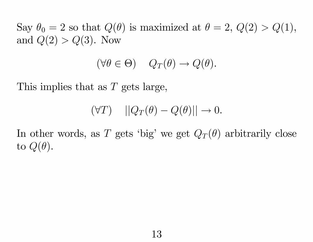
Say 0 = 2 so that ( ) is maximized at = 2, (2) (1),and (2) (3). Now

( ) ( ) ( ).

This implies that as gets large,

( ) || ( ) ( )|| 0.

In other words, as gets ‘big’ we get ( ) arbitrarily closeto ( ).

13

Now suppose that even for very large , ( ) is not maxi-mized at 2 but say at 1. Then we have

( ) (1) (2) 0.

Then under regularity condition 2 (q.v. §1.2) this would imply(1) (2) 0, a contradiction.

Hence the estimator ˆ .

Here principle is an example of the extremum principle.This principle involves either maximization or minimizationof the criterion function. Examples include the maximum like-lihood (maximization) and nonlinear least squares (minimiza-tion) methods.

14

2 Overview of Convergence Conceptsfor Non-stochastic Functions

Most estimators involve forming functions using the data avail-able. These functions of data can be viewed as sequences offunctions, with the index being the number of data points avail-able.

With su cient data (large samples), these functions of sampledata converge ‘nicely’ (assuming certain conditions), ensuringthat the estimators we form have good properties, such as ‘con-sistency ’ and ‘asymptotic normality’.

15

In this section, we examine certain basic concepts about con-vergence of sequences of functions. The key idea here is thatof uniform convergence; we shall broadly motivate why thisnotion of convergence is required for us.

For simplicity, we look at non-stochastic functions and non-stochastic convergence notions. Broadly construed, the sameideas also apply to stochastic functions–analogous conver-gence concepts are applicable in the stochastic case.

16

2.1 Pointwise Convergence

Let : be a sequence of real valued functions. Foreach form a sequence

©( )ª

=1. Let be the set

of points for which ( ) converges.

( ) ( ) := lim ( )

We then call ( ) a ‘limit function’, and say ‘©

( )ª

=1con-

verges pointwise to ( ) on ’.

Nota bene, pointwise convergence is not enough to guaranteethat if has a property (continuity, di erentiability, etc.) thatthat property is inherited by .

17

Inheritance requires uniform convergence. Usually, this is asu cient condition for the properties of being shared by thelimit function. Some of the properties we will be interested inare summarized below:

• Does ‘( ) ( ) is continuous’ = ‘ ( ) is continuous’?

• Does ‘( ) lim0

( ) = ( 0)’ = ‘ lim0

( ) = ( 0)’?

I.e. does lim0

lim ( ) = lim lim0

( )?

• Does lim R( ) =

Rlim ( ) =

R( ) (where ( )

is the limit function)?

The answer to all three questions is: No, not in general. Thepointwise convergence of ( ) to ( ) is generally not su -

18

cient to guarantee that these properties hold. This is demon-strated by the examples which follow.

19

Example 1Consider ( ) = (0 1).Here, ( ) is continuous for every , but the limit functionis:

( ) =

(0 if 0 1

1 if 0 = 1

This is discontinuous at = 1.

20

Example 2Consider

( ) =+

( R).

Then the limit function is ( ) = lim ( ) = 0 for each fixed

. This implies that lim lim ( ) = 0.

But we have lim ( ) = 1 for every fixed . This implies that

lim lim ( ) = 1 6= lim lim ( ) = 0.

21

Example 3Consider ( ) = (1 2) (0 1). Then the limitfunction is2

( ) = lim ( ) = 0

for each fixed . This implies thatR 10

( ) = 0. But we alsoget

lim

Z 1

0

( ) = lim2 + 2

=1

2.

2See Rudin, Chapter 3 for concepts relating to convergence of se-quences.

22

2.2 Uniform Convergence

A sequence of functions { } converges uniformly to onif

( 0)( )( )( ) | ( ) ( )|

where depends on but not on , i.e.,

( ) ( ) ( ) ( ) + .

Intuitively, for any as gets large enough, ( ) lies ina band of uniform thickness around the limit function ( ).

23

Note that the convergence displayed in the examples in §2.1did not satisfy the notion of ‘uniform’ convergence.

We have theorems that ensure that the properties of inheri-tance referred to in §2.1 are satisfied when convergence is uni-form.3

3See Rudin, Chapter 7. Theorems 7.12, 7.11, and 7.16 respectivelyensure that the three properties listed in §2.1 hold.

24

3 Applications of the AnalogPrinciple

25

3.1 Moment Principle

In this case, the criterion function is an equation connectingpopulation moments and 0.

=¡population moments of [ ]

¢= 0 at = 0. (1)

Thus, the property here is not maximization or minimization(as in the extremum principle), but setting some function ofthe population moments (generally) to zero at = 0, so thatsolving equation 1 we get the estimator:

ˆ =¡sample moments [y,x]

¢

26

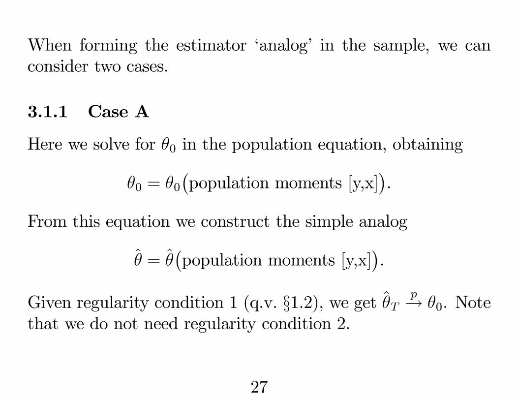
When forming the estimator ‘analog’ in the sample, we canconsider two cases.

3.1.1 Case A

Here we solve for 0 in the population equation, obtaining

0 = 0

¡population moments [y,x]

¢.

From this equation we construct the simple analog

ˆ = ˆ¡population moments [y,x]

¢.

Given regularity condition 1 (q.v. §1.2), we get ˆ 0. Notethat we do not need regularity condition 2.

27

Example 4 (OLS) 1. The model.

= 0 + E( ) = 0

Var( ) = 2 E( 0 ) = 0

E( 0 ) =X

positive definite E( 0 ) =X

2. Moment principle (criterion function). In the population

E( 0 ) = 0or 0 = 0

0 +0

:P

=P

0 + 0

0 =P 1P .

28

3. Analog in sample.

ˆ =

μP 0 ¶ 1μP ¶Now, r.h.s.

¡P ¢ 1P. Thus, ˆ 0.

29

3.1.2 Case B

Here we form the criterion function, form the sample analogfor the criterion function, and then solve for the estimator.

We require condition 1 (q.v. §1.2) and uniform convergence(condition 2) to get consistency of the estimator – i.e. forˆ

0.

Example 5 (OLS – another analogy)

1. The model. As in §3.1.1.

2. Moment principle (criterion function). In the population: E( 0 ) = 0.

30

3. Analog in sample. Here we define an ample analog of :b = ˆ

This mimics in the criterion function, so that we canform the sample analog of the criterion function by sub-stituting b for in the expression for above:

=1X

( ˆ) = 0

4. The estimator. Here we pick ˆ by solving from toarrive at the relation

1X=

μP ¶ˆ.

31

Remarks.

• Recall that in Case A (q.v. §3.1.1) we did not form ,but first solved for 0 and then formed ˆ directly, skippingstep 3 of Case B.

• Observe that when = 1,

ˆ =

Pis the mean.

• OLS can also be interpreted as an application of the ex-tremum principle (s.v. §3.2).

32

3.2 Extremum Principle

We saw in §1.3 that under the extremum principle, property Pprovides that ( ) achieves a maximum or minimum at = 0

in the population.

This principle underlies the nonlinear least squares (NLS) andmaximum likelihood estimation (MLE) methods. As theirnames suggest, MLE choose to be a maximum while NLSchoose to be the minimum.

33

The OLS estimator can be seen as a special case of the NLSestimators, and can be viewed as an extremum estimator.

In this section we analyze OLS and NLS as extremum estima-tors. MLE is examined in more detail in §4.

34

Example 1 (OLS as an extremum principle)

1. The model. We assume the true model

= 0 += = +

¡( 0 ) +

¢= ( )0( ) = ( 0 )0 0 ( 0)

+ 2 0 ( 0) +0 .

2. Criterion function.

= E¡( )0( )

¢From model assumptions, we have E( 0 ) = 0. Thus

= ( 0)0X( 0) +

2 .

35

So is minimized (with respect to ) at = 0.

Here, then, is an example of the extremum principle.It is minimized when = 0 (the true parameter vector).

3. Analog in sample. A sample analog of the criterion func-tion is constructed as

=1X

=1

( )0( 0 ).

36

We can show that this analog satisfies the key requirementof the analog principle:

plim = plim1X

=1

( )0( 0 )

= ( 0)0X( 0) +

2 =

(Assuming conditions for application of some LLN aresatisfied; q.v. Part I of these lectures.)

4. The estimator. We pick ˆ to minimize . Under stan-dard regularity conditions, we can show that we get con-tradiction unless ˆ 0.

37

Example 2 (NLS as an extremum principle)

1. The model. We assume that the following model holds inthe population:

= ( ; 0) + (non-linear model)= = ( ; ) +

¡( ; 0) ( ; )

¢+ .

Assume ( ) i.i.d. Then implies that

( ) ( ; ).

38

2. Criterion function. Choose the criterion function as

= E¡

( ; )¢2= E

¡( ; 0) ( ; )

¢2+ 2 .

Then is minimized at = 0 (a true parameter value).If = 0 is the only such value, the model is identifiedwith respect to the criterion – regularity condition 1(q.v. §1.2) is satisfied.

3. Analog in sample.

( ) :=1X

=1

¡( ; )

¢2As in the OLS case, we can show that plim = .

39

4. The estimator. We construct the NLS estimator as

ˆ = argmin ( ).

We thus choose ˆ to minimize ( ). Reductio ad ab-surdum verifies that

( 0) ( 0)

and( ) ( ) ( ) = ˆ .

40

Remark. The NLS estimator could also be derived as amomentestimator, just as in the OLS example (q.v. §3.1).

1. The model. Same as the non-linear model above. Wehave ( ; ).

2. Criterion function. = E¡ · ( ; )

¢= 0. Note that

this is only one implication of . We may now write

( ; ) == = E

¡( ; ) · ( ; )

¢= 0

3. Analog in sample.

:=1X

=1

¡( ; )

¢ · ( ; )

41

4. The estimator. Find which sets = 0 (or as close tozero as possible).

4 Maximum Likelihood

The maximum likelihood estimation (MLE) method is an ex-ample of the extremum principle. In this section, we look at theideas underlying MLE and examine the regularity conditionsand convergence notions in more detail for this estimator.

42

4.1 The Model

Suppose that the joint density of data is

( ; 0) · ( | ; 0) · ( ).

Assume that is ‘exogenous’ – i.e. the density of is unin-formative about 0. Also assume random sampling. We arriveat the likelihood function

L =Y=1

( ; 0).

Taking ( ) as data, L becomes a function of 0. The loglikelihood function is

lnL =X=1

ln ( ; ) =X=1

ln ( | ; ) +X=1

ln ( ).

43

4.2 Criterion Function

In the population define the criterion function as

= E 0

¡ln ( ; )

¢=

Z ¡ln ( ; )

¢( ; 0)d d .

(We assume this integral exists.)We pick the that maximizes L. Note that this is an extremumprinciple application of the analogy principle.

44

Claim. The criterion function is maximized at = 0.Proof.

E 0

μ( ; )

( ; 0)

¶= 1 becauseZ

( ; )

( ; 0)( ; 0)d d = 1.

45

Applying Jensen’s inequality, concavity of the ln function im-plies that

E¡ln( )

¢lnE( )

= E 0

μln

μ( ; )

( ; 0)

¶¶0

= ( ) E 0

¡ln ( ; )

¢E 0

¡ln ( ; 0)

¢.

We get global identification in the population if the inequalityis strict for all 6= .

46

4.3 Analog in Sample

Construct a sample analog of the criterion function as

:=1X

=1

ln ( ; ).

4.4 The Estimator and its Properties

We form the estimator as

ˆ := argmax

(we assume this exists).

47

Local form of the principle. In the local form, we use FOC andSOC to arrive at argmax . Recall that we have thecriterion function

( ) =

Zln ( ; ) ( ; 0)d = E 0

¡ln ( ; )

¢.

Maximization of the criterion function yields first and secondorder conditions:

FOC:Z

ln ( )( ; 0)d = 0

SOC:Z 2 ln ( ; )

0 ( ; 0) negative definite

48

Accordingly, we require for the sample analog:

1X=1

ln ( ; )= 0

1X=1

2 ln0 negative definite

For ‘local identification’, we require that the second order con-ditions be satisfied locally around the point solving the FOC.For ‘global’ identification, we need SOC to hold for every.

49

Either way (e.g. directly by a grid search or using the FO/SOCs),we have the same basic idea. For each , we pick ˆ such that

( ) (ˆ ) ( ).

Now if (ˆ ) (limˆ ) (uniform convergence), we get thecontradiction

(ˆ ) ( 0) –

assumed to be a maximum value – unless plim ˆ = 0.To be more precise, we must check whether

uniformly(almost surely).

It remains to cover certain concepts and definitions for randomfunctions.

50

5 Some Concepts and Definitions forRandom (Stochastic) Functions

In §5.1 we define random functions and examine some funda-mental properties of such functions. In §5.2 we define conver-gence concepts for sequences of random functions.

51

5.1 Random Functions and Some Properties

Definition 2 (Random Function)Let ( A ) be a probability space and let R . A realfunction ( ) = ( ) on × is called a random functionon if

( R1)( )

©: ( )

ªA.

We can then assign a probability to the event: ( ) .

52

Proposition. If ( ) is a continuous real-valued function on× where is compact, then

( ) sup ( ) and ( ) inf ( )

are continuous functions.Proof. See Stokey, Lucas, and Prescott, Chapter 3 for defini-tions of sup and inf , and for the proof of this proposition (q.v.

Theorem 3.6).

53

Proposition. If for almost all values of , ( ) is con-tinuous with respect to at the point 0, and if for all in aneighborhood of 0 we have¯̄

( )¯̄

1( ) ,

then

lim0

Z( )d ( ) =

Z( 0)d ( ).

I.e.lim

0

E¡( )

¢= E

¡( 0)

¢.

Proof. This is a version of a ‘dominated convergence theorem’.See inter alios Royden, Chapter 4.

54

Proposition. If for almost all values of and for a fixedvalue of

(a)( )

exists (in a neighborhood of ), and

(b)

¯̄̄̄( + ) ( )

¯̄̄̄2( ),

for 0 | | 0, independent of , thenZ( )d ( ) =

Z( )

d ( ).

I.e.

E¡( )

¢= E

( )¸.

55

5.2 Convergence Concepts for RandomFunc-tions

In Part I (asymptotic theory) we defined convergence conceptsfor random variables. Here we define analogous concepts forrandom functions.

Definition 3 (Almost Sure Convergence)Let ( ) and ( ) be random functions on for each

. Then ( ) almost surely converges to ( ) asif

( 0)©: lim | ( ) ( )| ª

= 1;

i.e. if for every fixed the set such that | ( )( )| , 0( ), has no probability.

56

= may have a non-negligible probability eventhough any one set has negligible probability. We avoid thisby the following definition.

Definition 4 (Almost Sure Uniform Convergence)( ) ( ) almost surely uniformly in if

sup | ( ) ( )| 0

almost surely as . I.e., if

( 0)( )©: lim sup | ( ) ( )| ª

= 1.

In this case, the negligible set is not indexed by .

57

Definition 5 (Convergence in Probability) Let ( ) and( ) be random functions on . Then ( ) ( ) in prob-

ability uniformly in on if

lim©sup | ( ) ( )| ª

= 0.

58

Theorem 1 (Strong Uniform Law of Large Numbers)Let { } be a sequence of random × 1 i.i.d. vectors. Let( ) be a continuous real function on . is compact (it

is closed and bounded, and thus has a finite subcover). Define

( ) = sup|| ||

sup | ( )|.

Let ( ) be the distribution of . Assume E[ ( )] . Then,

1X=1

( )a. s. unif.

Z( ) d ( ).

59

This is a type of LLN, and could be modified for the non-i.i.d.case. In that case, each has its own distribution , and wewould require that

(a)1X

=1

and

(b) sup1X

=1

E¡| ( )|¢1+ .

Then1X

=1

( )a. s. unif.

Z( )d ( ).

Note that we need a bound in either case on E[| ( )|].

60

References

1. Amemiya, Advanced Econometrics, 1985, Chapter 3.

2. Greenberg and Webster, Advanced Econometrics, 1991,Chapter 1.

3. Newey and McFadden, ‘Large Sample Estimation andHypothesis Testing’ in Handbook of Econometrics, 1994,Chapter 36, Volume IV.

4. Royden, Real Analysis, 1968, Chapter 4.

5. Rudin, Principles of Mathematical Analysis, 1976, Chap-ters 3 and 7.

61

6. Stokey, Lucas, and Prescott, Recursive Methods in Eco-nomic Dynamics, 1989, Chapter 3.

62