asymptotic dependence and exchange rate forecasting

Asymptotic dependence and exchange rate forecasting

Francisco Pinto-Avalos∗ Michael Bowe† Stuart Hyde‡

Abstract

This paper explores the relationship between commodity and exchange rate returns

in terms of their non-linear association and the ability of commodity prices to predict

exchange rates. Using a broad sample of commodity exporting economies we document

that the forecasting ability of commodity prices lies in the asymptotic dependence

relationship between commodity and exchange rate returns at a daily frequency. We

argue that the information located in the tail of the distributions is a key component

to describe the short-lived relationship between those variables.

Keywords: Exchange rates, commodity prices, asymptotic dependence, forecast-

ing.

EFM Classification: International finance. 610 - Currency Markets and Exchange

Rates

JEL Codes: F31, F37, C22, C53.

∗Corresponding author and presenter. The University of Manchester. Alliance Manchester Business

School, Booth Street West, Manchester, M15 6PB, UK. E-mail: [email protected]†The University of Manchester. Alliance Manchester Business School, Booth Street West, Manchester,

M15 6PB, UK. E-mail: [email protected]‡The University of Manchester. Alliance Manchester Business School, Booth Street West, Manchester,

M15 6PB, UK. E-mail: [email protected]

1 Introduction

Recent empirical studies (Ferraro et al. 2015, Foroni et al. 2015) provide evidence that changes

in commodity prices contain a degree of predictive power for exchange rate fluctuations. Both

the distribution of exchange rates and commodity prices, measured as a log-returns, exhibit

heavy tails, indicating the presence of extreme values in their sample distributions. Motivated

by the fact, this paper seeks to investigate the existence of an extreme connection between

the variables, examining whether asymptotic dependence underpins the predictive ability of

commodity prices for exchange rates. We investigate whether the documented predictive

ability of commodity prices applies to broad sample of commodity exporting economies, and

the frequencies at which it exists.

A number of recent studies analyse the tail behaviour of financial variables.1 Research

focusing on the information contained in the tails of the distribution explores the relation-

ship between two or more variables when linear correlation fails to detect the extent of the

association between them. The belief is that the information contained in the tails of the

distribution may contribute to explaining the degree of association between the variables. For

example, Cumperayot & De Vries (2017) demonstrate that measuring the asymptotic depen-

dence between exchange rates and classic monetary fundamentals allows one to explain how

large swings in exchange rates are related to sharp movements in monetary fundamentals.

This paper contributes to the literature on asymptotic dependence and its implications by

examining the relationship between exchange rates and commodity prices in a tail dependence

framework. We believe it is the first paper to attempt to synthesise these two literatures.

We highlight the role of asymptotic dependence as a central component of the ability of

commodity prices to predict exchange rates. In particular, our focus is to establish the

nature of the additional information contained in the tails of the distribution and its role in

exchange rate predictability. Our approach employs multivariate extreme value techniques.

We explore the occurrences of large movements in exchange and commodity prices and test if

they are asymptotically dependent. Measuring tail dependence enables us to determine the

extent to which large movement in exchange rates relate to their underlying fundamentals, in

this case, commodity prices. Our empirical approach is particularly relevant when variables

are known to exhibit fat-tailed distributions.

Our main results demonstrate that the asymptotic dependence between commodity prices

and exchange rates is significant when prices are measured contemporaneously and at a

1See Patton (2006) for a survey of studies implementing a copula approach. Patton (2012) surveys the

methodology and approaches to modelling the tail behaviour of financial variables.

1

daily frequency, while it reduces considerably when we use lagged values or data at a lower

frequency. Moreover, we also show that the predictive ability of commodity prices is highly

significant when we use contemporaneous daily observations. Using lagged or lower frequency

observations reduces the ability of commodity prices to forecast exchange rates. We maintain

that the nature of the documented asymptotic dependence is a key element in evaluating

the relationship between the two variables, and in particular it is the crucial element to

incorporate when analysing the ability of commodity prices to predict exchange rates.

2 Related literature

2.1 Exchange rates and Commodity prices

We now contextualise the contribution of this study in relation to the existing literature. Rossi

(2013) surveys the large research literature on nominal exchange-rate forecasting, including

models using commodity prices, and concludes that the random walk remains a difficult

benchmark to outperform (Meese & Rogoff 1983). She reports that linear models appear

the most successful and that results vary depending upon the set of predictors, the sample

period, the forecast evaluation method, and the forecast horizon. In this vein, several studies

focus upon the analysis of the statistical relationship between commodity prices and both

real and nominal exchange rates at a variety of frequencies. Conducting in-sample exercises

using quarterly frequency observations, Chen & Rogoff (2003) claim strong correlation and

cointegration between commodity prices and real exchange rates of several developed country

commodity exporters. Further, Cashin et al. (2004) provide evidence of the in-sample pre-

dictive power of commodity export prices to explain real exchange rates. They find evidence

of correlation and cointegration in around one-third of their sample of 58 economies using

observations at the monthly frequency.

Amano & van Norden (1995, 1998a,b) provide evidence in favour of the ability of com-

modity prices to explain exchange rates at a monthly frequency using cointegration analysis

applied to a subset of advanced economies. The 1995 study presents empirical evidence

linking the Canada-US real exchange rate with the terms of trade, reporting that the real

exchange rate is cointegrated with terms-of-trade variables (price of commodity exports rel-

ative to the price of manufactured imports), and that causality runs from the terms of trade

to the exchange rate. Moreover, a simple exchange rate equation performs better than a

random walk in post-sample forecasting exercises. In the 1998 study, the authors document

a robust and relationship between the real domestic price of oil and real effective exchange

2

rates for Germany, Japan and the United States. They attribute this effect to the real oil

price capturing exogenous terms-of-trade shocks and explain why these shocks may determine

long-term real exchange rates.

Chen (2002) finds that including commodity prices improves the out-of-sample forecasting

ability of fundamental-based models for nominal exchange rates at the monthly frequency in

the cases of Australia, Canada and New Zealand. However, the evidence is not completely

robust for the entire sample period under analysis. In contrast, Chen et al. (2010) using both

in-sample Granger-causality tests with time-varying parameters and out-of-sample forecast-

ing with rolling windows, document that nominal exchange rates (for commodity currencies)

help forecast commodity prices, but find no evidence for the reverse impact. Their study

analyses nominal exchange rates of Canada, Australia, New Zealand, South Africa, and

Chile (each relative to the US dollar) along with export-earnings-weighted commodity prices

for each country, at a quarterly frequency. They rationalise their findings in the context of a

present value model following Engel & West (2005).

While much of the earlier literature is based on low frequency sampling, some more

recent studies investigate the forecasting ability of commodity prices using daily and higher

frequency data. Zhang et al. (2016), using daily data from a sample of four economies

(Australia, Canada, Chile, Norway), document the in-sample ability of three commodity

prices (crude oil, gold, copper) to explain exchange rates. They employ both conditional

and unconditional causality measures and consider non-USD exchange rates, noting that the

documented relationship is stronger at short horizons and runs mainly in the direction of

commodity prices to exchange rates. Similarly, Foroni et al. (2015), using a mixed frequency

estimation based on both daily and monthly observations for a sample of advanced economies,

show that incorporating commodity prices improves the forecasting ability of fundamentals-

based exchange rate models.

Other recent papers extend the analysis to a broader sample of countries at a daily fre-

quency. Ferraro et al. (2015) examine the ability of oil prices to forecast exchange rates in

a one-step ahead, out-of-sample exercise for five commodity exporter economies (Australia,

Canada, Chile, Norway, and South Africa). However, Akram (2004) shows that the value

of the Norwegian krone value against a European basket of currencies is not correlated with

the oil price. Kohlscheen et al. (2017) find a strong correlation between changes in the nom-

inal exchange rate and a daily index of export commodity prices for 11 countries using a

panel dataset.2 Both studies provide evidence of the forecasting ability of contemporaneous

2Australia, Canada, Norway, Brazil, Chile, Colombia, Mexico, Peru, South Africa, Russia and Malaysia.

3

commodity prices to beat a RW model in out-of-sample exercises using observations at a

daily frequency, while they also show that the forecasting ability tends to be weaker using

monthly data, and completely disappears at a quarterly frequency. In addition, both studies

find that only contemporaneous commodity prices outperform the RW model and confirm

that there is little evidence of out-of-sample prediction using lagged commodity prices. In

particular, Ferraro et al. (2015) argue that any forecasting ability comes from the short-lived

relationship between commodity prices and exchange rates, therefore, including contempora-

neous observations at a daily frequency is a crucial component in capturing the relationship

between these variables.

2.2 Higher moments in exchange rate distributions

An alternative line of literature analyses the role of higher moments in the exchange rate

distribution by modelling tail relationships using extreme value theory, often adopting a

copula methodology. Patton (2006) studies the tail behaviour of the Japanese yen and the

German mark. His results indicate exchange rate movements located in the tails of the

distribution are asymmetric, and that the degree of association between these currencies

tends to be higher during periods of currency depreciation in comparison to episodes of

appreciation. Similarly, Yang & Hamori (2014) also find asymmetric effects during periods

of appreciation and depreciation when analysing the tail behaviour of the Euro, Japanese

yen and British pound in relation to the gold price. Using a time-varying copula approach

to analyse the tail relationship between the Japanese Yen and the Euro, Dias & Embrechts

(2010) argue that time-varying estimation provides additional information about the tail

dependence between the variables. While this literature exploits information in the tails for

examining the relationship between exchange rates and other financial assets, Cumperayot

& De Vries (2017) explore the ability of monetary fundamentals to forecast exchange rates.

Their main results show that information located in the tails of the distributions of exchange

rates and monetary fundamentals contributes to explaining the relationship between the

variables.

This paper seeks to synthesis these two literatures, and to the best of our knowledge,

our research is the first to study the link between exchange rates and commodity prices in

such a tail dependence framework. The novelty of our contribution lies in measuring the

degree of asymptotic dependence and how this relationship contributes to explain the ability

of commodity prices in forecasting exchange rates. This analysis of the tail behaviour of

exchange rates and commodity prices may be highly relevant in terms of policy considera-

tions for the subset of commodity exporting economies which document a close relationship

4

between exchange rates and commodity prices.

3 Commodity exporter economies

Commodity price shocks play a key role in the transmission of global shocks to domestic

economies. As discussed by Agenor & da Silva (2019), the effect of commodity prices is

particularly relevant for the economic outlook of commodity exporting economies. On the

one hand, in the short run, a negative commodity price shock reduces the export revenues

which translates to a lower foreign currency inflows (typically U.S. dollars) arriving into the

commodity exporting economy. As a result, the exchange rate of those economies tends to

depreciate. On the other hand, in long run, a negative commodity price shock is interpreted

as a worsening in the economic outlook of the commodity exporting economies. The de-

terioration in future economic expectations in commodity exporting countries discourages

investment in those countries, as a result capital flows tend to run from these economies and

their exchange rate tends to depreciate.

As pointed out by the International Monetary Fund (2017), the relationship between

exchange rates and commodity prices is especially sensitive in the case of commodity ex-

porting economies. It is particularly important to understand commodity price shocks as

an element which conveys information into commodity exporting economies and ends up

generating changes to the value of their currencies. This relationship has been particularly

notorious during the commodity price super-cycle taking place from the 2000’s. De Gre-

gorio (2012) shows that, during prolonged episodes of high commodity prices, commodity

exporting economies exhibit large and persistent current account deficits due to the massive

capital inflows which aim to invest in the commodity sector. In this case, massive capital

inflows lead exchange rate appreciations. Following this logic, shocks generated in commod-

ity markets produce changes in the domestic economic expectations of commodity exporting

economies. Then, that change in the future outlook of the commodity sector drive capital

flows movements which finally impact exchange rates. The relationship between commodity

prices and capital flows is consistent with the finding of related papers, such as Reinhart &

Reinhart (2009) and Byrne & Fiess (2016).

Given our focus on the relationship between commodity prices and exchange rates, the

sample of countries we include in this paper satisfy two conditions: (1) commodities must

represent a significant proportion of the country’s exports, and (2) countries must have a free

floating exchange rate regime.Therefore, the sample of economies we include in the analysis

5

is identified to be among the commodity exporting economies (International Monetary Fund

2012). Moreover, in general, the exports of these countries are both poorly diversified and

mainly consist upon one or two main commodities. Countries with poorly diversified exports

develop a high degree of economic dependence upon commodities. In addition, all of the

countries in the sample have adopted a free floating exchange rate regime.

Table 1 reports some descriptive statistics of the economies included in the sample. For

each country in the sample the table shows a set of commodity related indicators during three

different periods of time: 2000-2005, 2006-2011, and 2012-2017. The indicators highlight the

relevance of commodity exports for the economies of the sample. As we observe, commodity

exports represent a high percentage of the total exports for all of the countries. Moreover,

the commodity sector is a highly relevant one for the whole economy. On average, around

15% of GDP is represented by the commodity sector. Additionally, the table also shows the

main product exported by each country, which represent a high proportion of the commodity

exports. All in all, the information exhibited in table 1 puts in perspective the relevance the

commodity exports for the countries under analysis. It is worth noting that, although, oil

seems to be less relevant for the case of Brazil, that country is one of the top ten oil producers

around the globe and it is the biggest oil producer in the region.3 The oil industry in Brazil

is also important for domestic investment and attracts foreign capital into the country.

3.1 Some empirical facts about returns

It is a well established empirical fact that the returns of many asset classes tend to follow

leptokurtic distributions. This distribution characterised by higher kurtosis and a greater

likelihood of observing extreme values in comparison to the normal distribution. As a result,

distributions describing returns tend to exhibit fat tails which is indicative of this higher

probability of observing extreme values. This fat-tailed phenomena also characterises ex-

change rate log-returns and commodity log-returns. Indeed, evidence on the growing degree

of financialisation of commodity markets since the 2000’s (Buyuksahin & Robe 2014, UNC-

TAD 2011) shows that commodities have been actively included in investment portfolios.

Thus, commodity returns, interpreted as another financial asset, may be expected to exhibit

fat-tailed distributions.

As an illustration, figure 1 plots the histograms of the US dollar - Chilean peso (USDCLP)

exchange rate in log-returns (left-hand side panel) and the copper price in log-returns (right-

3According to the U.S. Energy Information Administration (EIA). See table in appendix A for more details

about the World’s Top Oil Producers.

6

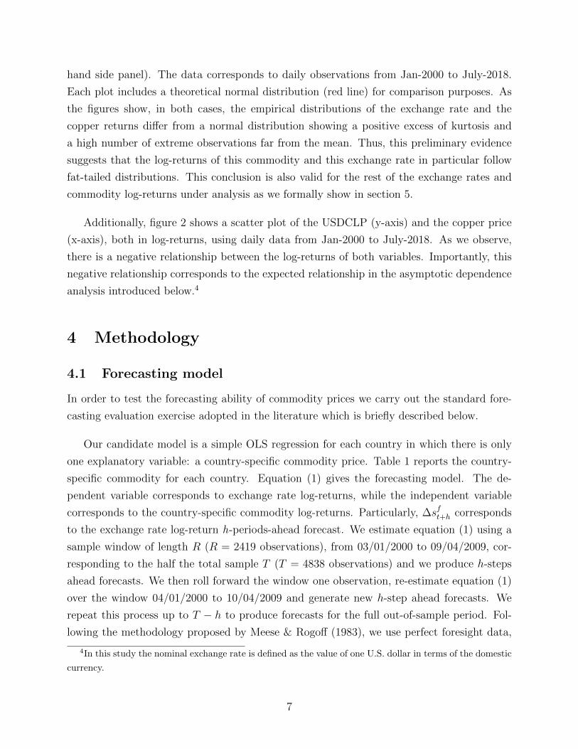
hand side panel). The data corresponds to daily observations from Jan-2000 to July-2018.

Each plot includes a theoretical normal distribution (red line) for comparison purposes. As

the figures show, in both cases, the empirical distributions of the exchange rate and the

copper returns differ from a normal distribution showing a positive excess of kurtosis and

a high number of extreme observations far from the mean. Thus, this preliminary evidence

suggests that the log-returns of this commodity and this exchange rate in particular follow

fat-tailed distributions. This conclusion is also valid for the rest of the exchange rates and

commodity log-returns under analysis as we formally show in section 5.

Additionally, figure 2 shows a scatter plot of the USDCLP (y-axis) and the copper price

(x-axis), both in log-returns, using daily data from Jan-2000 to July-2018. As we observe,

there is a negative relationship between the log-returns of both variables. Importantly, this

negative relationship corresponds to the expected relationship in the asymptotic dependence

analysis introduced below.4

4 Methodology

4.1 Forecasting model

In order to test the forecasting ability of commodity prices we carry out the standard fore-

casting evaluation exercise adopted in the literature which is briefly described below.

Our candidate model is a simple OLS regression for each country in which there is only

one explanatory variable: a country-specific commodity price. Table 1 reports the country-

specific commodity for each country. Equation (1) gives the forecasting model. The de-

pendent variable corresponds to exchange rate log-returns, while the independent variable

corresponds to the country-specific commodity log-returns. Particularly, ∆sft+h corresponds

to the exchange rate log-return h-periods-ahead forecast. We estimate equation (1) using a

sample window of length R (R = 2419 observations), from 03/01/2000 to 09/04/2009, cor-

responding to the half the total sample T (T = 4838 observations) and we produce h-steps

ahead forecasts. We then roll forward the window one observation, re-estimate equation (1)

over the window 04/01/2000 to 10/04/2009 and generate new h-step ahead forecasts. We

repeat this process up to T − h to produce forecasts for the full out-of-sample period. Fol-

lowing the methodology proposed by Meese & Rogoff (1983), we use perfect foresight data,

4In this study the nominal exchange rate is defined as the value of one U.S. dollar in terms of the domestic

currency.

7

meaning that we include realised values of commodity returns in the forecasting exercises.

For this reason, the approach is also known as a pseudo out-of-sample forecasting, since in

real life situations it is not possible to know tomorrow’s value of commodity returns. We set

short-term forecast horizons at h = 1, 2, 3, 4, 5, 10 periods ahead. Following the exchange rate

forecasting literature, related studies using daily observation mostly focus on short-term hori-

zons (e.g.: Ferraro et al. (2015) and Kohlscheen et al. (2017) use 1-step ahead forecast using

daily commodity prices), while others studies using lower frequency observation, quarterly

or annual observations, set longer forecast horizons (see Rossi (2013)).

∆sft+h = αt + βt∆pt+h, t = R,R + 1, ..., T − h. (1)

We select the RW model as a benchmark against which to contrast our commodity-based

forecasts. According to Rossi (2013), the RW model without drift is the toughest benchmark

to beat in out-of-sample forecast exercises.

In order assess the out-of-sample forecasting ability of the models, we statistically compare

the root mean square forecast error (RMSE) of both models using the Diebold-Mariano (DM)

test. Giacomini & White (2006) show that the DM test is valid to compare the out-of-sample

forecasts of two nested models when the length of the estimation windows is constant. As a

robustness check we also evaluate the forecasting ability of the models using the Clark-West

(CW) test. The CW test corrects the RMSE taking in account noise that may be generated

due to parameter uncertainty.

4.2 Fat-tailed distribution in returns: Tail indexes

Before considering the extent of asymptotic dependence between two random variables, we

need to demonstrate that the variables under analysis exhibit heavy-tail distributions.

In order to test whether exchange rates and commodity returns follow fat-tailed distri-

butions we implement two non-parametric approaches: the Hill tail index (Hill 1975) and a

tail index indicator (Dekkers et al. 1989) shown in equations (2) and (3), respectively.

H =1

k

k∑i

log

(X(i)

X(k)

)(2)

γ = 1 +H +1

2

(MH

H − MH

), (3)

8

These non-parametric indicators consider order statistics of a random variable X of length

n, such that X is sorted in descending order as follows X(1) ≥ X(2) ≥ . . . ≥ X(n). Then,

the indicators only include the information located above the threshold represented by X(k),

where k corresponds the number of observations above the threshold. The variance of both

indicators is asymptotically normally distributed and given by H2 and 1 + γ2 for the H and

γ estimator, respectively. When tail indices display positive values and the confidence bands

do not include zero, the indicators suggest that statistically log-returns follow a heavy-tail

distribution.

The Hill tail index is an unbiased estimator and it is also more efficient in comparison

to other alternative tail index indicators as pointed out by Tsay (2010) and Cumperayot

& De Vries (2017). However, the indicator assumes that the data comes from a fat-tailed

distribution. In contrast, the γ tail index indicator is more flexible since it does not assume

a priori any specific distribution in the data.

4.3 Asymptotic dependence

In order to analyse the information contained in the tail of the log-returns distribution (i.e.

extreme values) and how those observations are related in a multidimensional framework the

related literature focuses on the concept of tail dependence. Tail dependence measures the

probability that extreme values of one random variable occur given that extreme values of

another random variable simultaneously happen. In other words, it is a measure of the joint

probability that large changes in two random variables take place simultaneously. Previous

studies provide a variety of procedures to estimate the tail dependence of two random vari-

ables. A common approach in finance focuses on modelling the whole join distribution of two

or more variables using the copula methodology. Under that approach, the idea is to model

the entire dependence structure between two random variables. The asymptotic dependence

method we implement in this paper, also known as the limit copula, is a more specific way

to analyse the probability of occurrence of large movements in two variables and it is also

an alternative and simplified standard procedure to model only the tail behaviour of two

random variables.

The relevance of the asymptotic dependence analysis is due to its contribution to explain

the relationship between two variables by taking in account the link between them based

on the information contained in the tails of the distribution. This is particularly relevant

when two (or more) variables seem to show a low degree of correlation, but most of the

relationship is driven by the information contained in the tails. For instance, this is the case

9

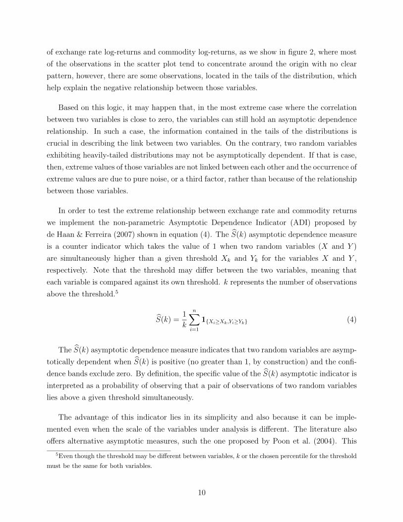
of exchange rate log-returns and commodity log-returns, as we show in figure 2, where most

of the observations in the scatter plot tend to concentrate around the origin with no clear

pattern, however, there are some observations, located in the tails of the distribution, which

help explain the negative relationship between those variables.

Based on this logic, it may happen that, in the most extreme case where the correlation

between two variables is close to zero, the variables can still hold an asymptotic dependence

relationship. In such a case, the information contained in the tails of the distributions is

crucial in describing the link between two variables. On the contrary, two random variables

exhibiting heavily-tailed distributions may not be asymptotically dependent. If that is case,

then, extreme values of those variables are not linked between each other and the occurrence of

extreme values are due to pure noise, or a third factor, rather than because of the relationship

between those variables.

In order to test the extreme relationship between exchange rate and commodity returns

we implement the non-parametric Asymptotic Dependence Indicator (ADI) proposed by

de Haan & Ferreira (2007) shown in equation (4). The S(k) asymptotic dependence measure

is a counter indicator which takes the value of 1 when two random variables (X and Y )

are simultaneously higher than a given threshold Xk and Yk for the variables X and Y ,

respectively. Note that the threshold may differ between the two variables, meaning that

each variable is compared against its own threshold. k represents the number of observations

above the threshold.5

S(k) =1

k

n∑i=1

1{Xi≥Xk,Yi≥Yk} (4)

The S(k) asymptotic dependence measure indicates that two random variables are asymp-

totically dependent when S(k) is positive (no greater than 1, by construction) and the confi-

dence bands exclude zero. By definition, the specific value of the S(k) asymptotic indicator is

interpreted as a probability of observing that a pair of observations of two random variables

lies above a given threshold simultaneously.

The advantage of this indicator lies in its simplicity and also because it can be imple-

mented even when the scale of the variables under analysis is different. The literature also

offers alternative asymptotic measures, such the one proposed by Poon et al. (2004). This

5Even though the threshold may be different between variables, k or the chosen percentile for the threshold

must be the same for both variables.

10

measure allows capturing the extreme linkage between two random variables by identifying

asymptotic dependence relationships and also by quantifying its degree of association. A

disadvantage of this approach is that the two random variables included in the analysis need

to be measured in the same scale. Additionally, as Fernandez (2008) notes, the Poon et al.

(2004)’s measure tends to provide biased results since it tends to reject the null hypothesis of

asymptotic dependence. In this sense, Fernandez (2008) concludes that the copula analysis,

and therefore the empirical copula analysis which corresponds to the de Haan & Ferreira

(2007) indicator implemented here, is a more suitable approach to measure the degree of

asymptotic dependence between two random variables.

5 Results

This section reports the results of the out-of-sample forecast and the asymptotic dependence

measure. The data corresponds to daily observations of nominal exchange rates and commod-

ity prices, both measured in log-returns, from 01/Jan/2000 to 18/Jul/2018. The countries

under analysis and the country-specific commodity prices are shown in table 1. The nominal

exchange rate is defined using the U.S. dollar as the base currency.

5.1 Out-of-sample forecasts

This section describes the results of the out-of-sample exercises using the forecasting model

introduced in equation 1.

Commodity-based models vs. random walk models

Table 2 presents the RMSE ratio between the commodity-based model (numerator) and a

RW model without drift (denominator) for the countries under analysis (in rows) and for

different forecast horizons (in columns). The results show that in all cases and for every

forecast horizon the commodity-based model forecasts better than the driftless RW model.

In addition, the Diebold-Mariano test indicates that the MSFE of the commodity-based

model is statistically lower, at 1% level, than the MSFE of the driftless RW model.

Similarly, as table 3 shows, the conclusions remain the same when comparing the fore-

casting ability of the commodity-based models against a RW model with drift. In this case,

the commodity-based models forecast better than a RW model with drift and the difference

in predictive power is statistically significant at 1% according to the Diebold-Mariano test.

11

Our results are consistent with previous findings. For instance, Ferraro et al. (2015) and

Kohlscheen et al. (2017) show that commodity-based models also beat the RW model, both

with and without drift, using daily observations.

5.2 Robustness tests

In order to test the statistical robustness of our results, we assess the forecasting ability of

the commodity-based models using the Clark-West test as an alternative statistical measure.

Tables 4 and 5 report the RMSE ratios using the driftless RW model and the RW with drift,

respectively. As the tables show, our results remain valid, meaning that the commodity-based

models produce lower MSFEs in comparison to the RW model with and without drift and

that difference is statistically significant at 1%.

Further we also test the robustness of our results by implementing the same out-of-sample

forecasting exercises but using an alternative definition of the base currency. Tables 6 and

7 show the results using the euro (EUR) and the pound sterling (GBP), as the currency

base, respectively. From the results, it is possible to hold that the findings generally remain

the same even after using an alternative base currency definition. The forecasting ability of

commodity-based models is still significant even when the US dollar is not the base currency.

Some minor exceptions appear in the case of Peru when the base currency is GBP or EUR,

and also in the case of South Africa using EUR as the base currency where the evidence is

only marginally significant at 10% level. Overall, the results of this robustness exercise show

that the forecasting ability of commodity prices is not only limited to the dollar as a base

currency, thus its predictive power goes beyond a mere dollar effect.

In addition, our results are robust to unobservable global factor affecting both exchange

rates and commodity returns. In order to test for the the effect of that potential factor we

replicate the out-of-sample exercise using exchange rate returns which are orthogonal to the

change in the VIX index. We include the VIX index since it is variable available at daily

frequency which accounts for global risk aversion which may be affecting both exchange rates

and commodity returns. Table 8 shows the results. As we can see, after controlling for the

effect of a global common factor, the conclusion remains the same even and we can hold

that commodity returns forecast better than a random walk model without drift for all the

countries in the sample.

12

5.2.1 Lagged commodity prices

In order to perform a truly out-of-sample exercise we use lagged commodity prices rather

than contemporaneous prices and replace equation (1) with equation (5).

∆sft+h = αt + βt∆pt, t = R,R + 1, ..., T − h. (5)

We estimate equation (5) using a sample window of length R (R = 2419 observations),

from 04/01/2000 to 10/04/2009, corresponding to the half the total sample T (T = 4838

observations) and we produce h-steps ahead forecasts. We then roll forward the window

one observation, re-estimate equation (5) over the window 05/01/2000 to 11/04/2009 and

generate new h-step ahead forecasts. We repeat this process up to T −h to produce forecasts

for the full out-of-sample period.

Table 9 depicts the results comparing the commodity-based models with a RW without

drift. As the results show, the forecasting ability of commodity prices disappears when

the explanatory variable is replaced by its lagged values. This evidence shows that the

commodity-based model using lagged commodity prices cannot beat the driftless RW.

On the contrary, when testing the commodity-based model using lagged commodity prices

against a RW model with drift the evidence supports the forecasting ability of lagged com-

modity prices. Table 10 shows that the commodity based model using lagged commodity

prices forecast better than a RW with drift and the results are statistically significant.

The evidence of the forecasting ability of our commodity-based model is closely related to

the findings of Ferraro et al. (2015) and Kohlscheen et al. (2017). They similarly highlight that

lagged commodity prices exhibit a lower forecasting ability in comparison to contemporaneous

values. In particular, the forecasting evidence of commodity prices disappears when the

benchmark is the driftless RW, while they show that there is still some evidence in favor of

commodity-based models to forecast better than the RW with drift.

5.2.2 Using low frequency data

In this section we analyse the forecasting ability of commodity based models using low fre-

quency observations. Following the standard procedure adopted in Ferraro et al. (2015), we

compute monthly and quarterly observations using the end-of-sample daily frequency. Ac-

cording to Rossi (2013), using end-of-sample observations implies a harder task in finding

forecasting ability in comparison to computing a monthly or quarterly average from daily

observations.

Table 11 presents the results using contemporaneous commodity prices at monthly fre-

13

quency and the driftless RW model as a benchmark. As can be observed, the forecasting

ability of the commodity-based model decreases in comparison to the daily data case for most

of the countries in our analysis. In general terms, there is no statistical evidence, or it is only

marginally significant at 10%, in favour of commodity prices. However, there is still some

predictive ability of commodity prices at 5% level of significance for the cases of Canada,

Chile and Norway.

We observe similar results when comparing the predictive ability of our commodity-based

model against a RW model with drift. As table 12 shows, the predictive ability of commodity

prices tends to reduce when comparing to the RW model with drift. Even though the

reduction in the forecasting ability decreases in comparison to daily frequency, there is still

a couple of highly significant cases, such as Canada and Norway, where commodity prices

forecast better that the RW with drift. However, as we previously noted, the statistical

significance in those cases comes from the fact the benchmark model, the RW with drift, it

is not the toughest benchmark to beat (Rossi 2013).

As with the daily observations previously, we then carry out a truly out-of-sample forecast

exercise, by including lagged commodity prices as the main explanatory variable, estimating

equation (5). Tables 13 and 14 present the results using the driftless RW model and the RW

model with drift, respectively. We find that the forecasting ability of the commodity-based

model completely disappears no matter which benchmark model we use. As shown, there is

no statistical significance in favour of lagged commodity prices to forecast better than the

benchmarks at a monthly frequency and this applies to every country under analysis.

In addition, replicating the previous exercises but using quarterly observations we reach

the same conclusions. First, by using contemporaneous commodity price observations, the

forecasting ability of commodity-based models reduces even further relative to the daily and

monthly frequency estimations, this holds for both benchmarks, the RW model without drift

(table 15) and RW with drift (table 16). An exception occurs in the case of Chile where

the predictive power of commodity prices is still highly significant. Second, the forecasting

ability of lagged commodity prices complete disappears for all countries in comparison to

daily and monthly frequency. This evidence holds either the benchmark model is defined as

a driftless RW (table 17) or a RW with drift (table 18).

The results of this section highlight the relevance of the data frequency in forecasting ex-

change rates using commodity-based models. We demonstrate that in reducing the frequency

of the data, from daily to monthly or quarterly observations, the forecasting ability of the

commodity prices decreases in both pseudo out-of-sample and truly out-of-sample exercises.

The results hold no matter the benchmark model we use, either the driftless RW or the RW

14

with drift. Our results are consistent with recent studies (Ferraro et al. (2015) and Kohlscheen

et al. (2017)) and reinforce the idea that using observations at a daily frequency is a crucial

element to capture the relationship between the variables. As we show, contemporaneous

commodity prices exhibit a higher forecasting ability in comparison to lagged commodity

prices. Thus, there is a short-lived relationship between the variables which is mostly cap-

tured based on the contemporaneous relationship between commodity prices and exchange

rates. Moreover, by lowering the data frequency the relationship between the variables tends

to vanish and, as a result, the forecasting power of commodity-based models also decreases.

This evidence highlights the relevance of daily observation in forecasting exchange rates. In

this sense, commodity price shocks affecting exchange rates are transitory and tend to di-

lute over time when economic agents internalise new information. Therefore, low frequency

observations are not able to capture those transitory information, consequently commodity

prices at a lower frequency are not useful in predicting exchange rates.

5.3 Fat-tailed distributions of log-returns

Table 19 reports the results of the Hill tail index defined in equation (2) for the case of both

the lower and upper log-returns tails, representing the most negative and positive log returns,

respectively. Confidence intervals at 95% level are also included in parenthesis. As shown,

for all cases and also for both upper and lower tails the indicator is positive and statistically

different from zero meaning that the distribution of log-returns of each variable follows a

fat-tailed distribution.

A more conservative evaluation of fat-tailed distributions is carried out using the Dekkers

et al. (1989) index. Table 20 presents the results of the γ tail index estimator introduced

in equation (3). As the table shows, most currencies and commodity prices exhibit heavily-

tailed distributions in both tails. Some exemptions appear in the case of upper tail for the

case of the Canadian dollar, the Norwegian krone and the copper price, while an exception

also appears in the lower tail for the the South African Rand. Despite the occurrence of those

exceptions, we can interpret the γ tail index estimator as a more strict measure to capture

the amount of information contained in the tails of the distribution.

Overall, these results allows us to conclude that there is information in the tails of the dis-

tribution which can be explored further by carrying out our asymptotic dependence analysis

in next section.

15

5.4 Asymptotic dependence

This section introduces the results of the asymptotic dependence measure based on de Haan &

Ferreira (2007). It is relevant to define some important cases under analysis before describing

the results. As we discuss in section 4, the ADI measures the asymptotic dependence between

a pair of random variables. In this study, there are 4 cases to analyse corresponding to the

combination of the two tails of each of the two random variables under analysis. Particularly,

we compute the ADI using nominal exchange rates and commodity prices, both in log-returns,

therefore, the four cases under analysis are the following:

• Case 1: Nominal exchange rate appreciation (lower tail of exchange rate log-return

distribution) and increase in country-specific commodity price (upper tail of commodity

log-return distribution).

• Case 2: Nominal exchange rate depreciation (upper tail of exchange rate log-return

distribution) and reduction in country-specific commodity price (lower tail of commod-

ity log-return distribution).

• Case 3: Nominal exchange rate appreciation (lower tail of exchange rate log-return dis-

tribution) and reduction in country-specific commodity price (lower tail of commodity


• Case 4: Nominal exchange rate depreciation (upper tail of exchange rate log-return

distribution) and increase in country-specific commodity price (upper tail of commodity


5.4.1 Asymptotic dependence using contemporaneous commodity prices

Table 21 reports the ADI estimation using daily contemporaneous commodity prices from

Jan-2000 to Jul-2018. Confidence bands are computed by bootstrap method using 5000

resampling iterations. As the table shows, the asymptotic dependence index is positive and

statistically significant for all countries in cases 1 and 2. On the contrary, for cases 3 and 4, the

index reduces in magnitude for all of the countries and becomes statistically non-significant

in most of the countries.

Results are in line with the theoretical relationship between commodity prices and ex-

change rates. As we discuss in section 3, commodity price shocks generate changes in com-

modity exporting economies which ultimately cause impacts on exchange rates. In particular,

16

a sharp decrease (increase) in the price of the country-specific exported commodity is associ-

ated with a deterioration (improvement) in the economic outlook of that commodity exporter

economy, as a result, a massive surge of capital flows flies from (enter to) the economy and,

as a consequence of this sudden deterioration (improvement) in economic confidence, a sharp

depreciation (appreciation) of the nominal exchange rate takes place.

Following this logic, the asymptotic dependence only makes sense when the variables are

negatively related such as in cases 1 (exchange rate appreciation and increase in commodity

price) and case 2 (exchange rate depreciation and a reduction in the commodity price).

Moreover, this expected negative relationship between the variables is empirically supported

in the data as we preliminary show in section 3.1. Importantly, cases 3 and 4 report low

values for ADI and, in general, show no statistical significance for most of the countries.

Our asymptotic dependence measure is robust to a set of alternative specifications. First,

the ADI is robust to commodity and exchange rates returns that are orthogonal to the VIX

index. As table 22 shows, cases 1 and 2 are statistically significant even after controlling

for the effect of common risk aversion, captured by the VIX index. This mean that the

asymptotic dependence measure goes beyond a mere risk factor that may move both exchange

rates and commodity returns. As expected, cases 3 and 4 are close to zero or statistically

non-significant.

Second, as commodity prices and exchange rates are measured in U.S. dollars, we also

show that the asymptotic relationship between the variables does not only reflect a dollar

effect. Tables 23 and 24 show the ADI defining the exchange rate using Euros and Pound

Sterling as a currency base, respectively. As we can see, the asymptotic dependence between

exchange rates and commodity returns remains significant for cases 1 and 2, while cases 3

and 4 are close to zero or statistically non-significant.

Third, due to the nature of time-series of log-returs, it may be the case that the effect

of heteroskedasticity in log-returns biases the result of the asymptotic dependence analysis.

Following the literature, we estimate our ADI measure controlling for the potential issue of

heteroskedastic in log-returns. To do so, we estimate our ADI measure using standardised

residual, which a are free of heteroskedasticity issues, for both commodity and exchange rate

returns. In order to compute the standardised residual we model the univariate conditional

variance for each return using a GARCH(1,1) model. As table 25 shows, the results after

controlling for heteroskedasticity remains the same, cases 1 and 2 are statistically significant

and they show an asymptotic dependence relationship around 10% on average, while cases 3

and 4 are much lower, close to zero, or statistically non-significant.

17

5.4.2 Interpretation of tail dependence between commodity prices and exchange

rates

The interpretation of the asymptotic dependence measure is based on the effect of unexpected

news over commodity markets. The arrival of unexpected news, or economic surprises, affect-

ing commodities markets generates sharp changes in commodity prices which are transmitted,

to some degree, to the commodity exporter economies impacting their exchange rates.

It is widely accepted that news has a significant impact on asset return volatility. Con-

sequently, episodes characterised by the frequent arrival of unexpected news are associated

with changes in asset prices and periods of high volatility of returns. Some studies show the

same logic also applies to commodity markets (Caporale et al. 2017; Frankel & Hardouvelis

1985; Roache & Rossi 2010) where the arrival of news has a significant impact on com-

modity price volatility. According to these studies, unexpected news affecting commodity

markets represents the main driver of large fluctuations in commodity prices. As a result,

large fluctuations in commodity prices translate to leptokurtic commodity log-return distri-

butions where extreme observations are more likely to take place generating fat tails in the

log-returns distributions.

Following the discussion about the transmission channel of external shocks into the do-

mestic economy (see section 3), large swings in commodity prices, which are driven by unex-

pected news in commodity markets, convey information to commodity exporting economies

by changing the perception of investors about the economic outlook of commodity exporting

economics, affecting capital flows and, ultimately, generating changes in domestic currencies.

In particular, the proposed measure of tail dependence allows us to quantify how extreme

values of exchange rates log-returns are related to extreme values of commodity log-returns.

Consequently, the relationship in the tails of the distribution provide us with an idea of how

much of the arrival of unexpected news in commodity markets are transmitted to exchange

rates. This point of view is also consistent with Ferraro et al. (2015) who interpret commod-

ity price shocks as the mechanism conveying information about macroeconomic news that

may affect exchange rates.

As an illustration of the above mechanism we provide an example using the copper price

and the Chilean exchange rate. In the particular case of the copper market, China’s copper

demand is considered as an important driver of the international copper price. The economic

activity in that country is closely related to changes in the copper price, therefore, news, or

economic surprises, about the current economic situation of China tend to impact the price

of cooper. Thus, it is expected that news, or surprises about economic activity in China,

18

generate a significant effect on copper price. Figure 3 shows the asymptotic dependence

indicator for the case of large decreases in copper prices and large depreciations in the Chilean

exchange rate (blue line), while the shaded grey areas correspond to those periods when

negative economic news (negative economic surprises) take place in China.6 As we can see

from figure 3, during episodes of negative economic surprises in China, we observe an increase

in our asymptotic dependence measure, meaning that bad news (or negative surprises) in

China are associated to large decreases in copper price, which, in turn, are linked to large

depreciation of the Chilean exchange rate. Therefore, it is possible to argue that, at least,

some part of the news (or economic surprises) affecting the copper market are also transmitted

to the Chilean exchange rate, via the copper price. Although China is a relevant global agent

affecting the copper market, it is worth noting that there is no perfect correlation between

events in figure 3 and our asymptotic dependence measure, this is mainly because surprises

about economic activity in China only represent a fraction of the shocks affecting the copper

market with other elements also playing a role in explaining changes in the international

price of copper.

5.4.3 Asymptotic dependence using lagged commodity prices

Table 26 shows the ADI estimation using one period lagged commodity prices at a daily

frequency. The results show that for cases 1 and 2 the asymptotic dependence considerably

reduces in magnitude in comparison to the case of contemporaneous commodity prices and,

for the case of some countries, the indicator is no statistically different to zero. In cases

3 and 4 there is certain significance for some countries, however the ADI tends to be low

around 5% on average, and importantly, tends to be as low as cases 1 and 2. All in all, the

statistical significance of asymptotic dependence between nominal exchange rates and lagged

commodity prices at daily frequency is rather than weak, specially compared with the cases

1 and 2 of ADI using contemporaneous commodity prices.

5.4.4 Asymptotic dependence using low frequency data

Table 27 presents a comparison of the the asymptotic dependence between exchange rates

and contemporaneous commodity prices computed at daily, monthly and quarterly frequency.

As can be seen, most of the asymptotic dependence tends to vanish at a monthly frequency

6The asymptotic dependence indicator shown in this example corresponds to the ADI case 2 described on

page 16. The China surprise index corresponds to the Citigroup China Economic Surprise Index obtained

from Bloomberg.

19

and only few countries (Chile, Norway, Russia, and South Africa) still show at least some

degree of statistical significance in cases 1 or 2, while no significance at all in cases 3 and 4.

Similarly, in the case of quarterly frequency and contemporaneous observations, there is

no statistically significant asymptotic dependence between exchange rate and contemporane-

ous commodity prices for any of the countries in the sample. This set of results contrasts with

the evidence provided in Cumperayot & De Vries (2017) since they show that the asymp-

totic dependence between classical monetary fundamentals and exchange rates is still present

when the data frequency is reduced to quarterly observations. On the contrary, in our case,

commodity price shocks measured at lower frequency, either monthly or quarterly, tend show

no effect on large exchange rate movements.

In the same way, using lagged commodity prices and low frequency data (see table 28)

we observe similar results: the asymptotic dependence evidence complete disappears at both

frequencies, monthly and quarterly, for all of the countries in the sample.

5.4.5 Relationship between exchange rate forecasting ability and asymptotic

dependence

Our results allow us to draw two main conclusions. First, timing plays a key role in describing

the relationship between exchange rates and commodity prices. As we show, the forecasting

ability of commodity prices and also the asymptotic dependence between the variables tend

to be short-lived meaning that only contemporaneous observations can capture that relation-

ship. As we show, both, the out-of-sample forecasting ability of commodity prices and the

asymptotic dependence between exchange rates and commodity prices are highly significant

in contemporaneous terms, while both tend to disappear when lagged commodity prices are

included in the analysis.

Second, the relationship between commodity prices and exchange rate is transitory. As

we show, the forecasting ability of commodity prices and the asymptotic dependence between

the variables is highly significant when observations are included at a daily frequency. On

the contrary, the forecasting ability and the asymptotic dependence tend to disappear when

lower frequencies are included either using monthly or quarterly observations.

The interpretation of our results lies in the nature of the news affecting commodity mar-

kets. As we previously discuss, large swings in commodity prices are driven by unexpected

news arriving to that market. Our ADI measure captures how those news, which cause large

20

swings in commodity prices, are also related to large movements in exchange rates. Unex-

pected news are transitory, short-lived and vanish over time as economic agents internalise

those surprises.7 As we document, the asymptotic dependence and the forecasting ability

of commodity prices are highly significant using contemporaneous daily observations, while

there is a reduction in the statistical significance of both elements when we use lagged or

observations at a low frequency. Therefore, we argue that the information contained in the

tails of the distributions, which reflects the effect of transitory, short-lived news arriving to

the commodity markets, is a key component of the forecasting ability of commodity prices.

On the contrary, when there is no news transmission from commodity prices to exchange rate

(i.e.: no asymptotic dependence) the forecasting ability of commodity prices statistically re-

duces. Therefore the ability of commodity prices to forecast exchange rates is manly driven

by the asymptotic dependence relationship between those variables. In this sense, log-returns

located in the tails of the exchange rate and commodity price distributions convey crucial

information to describe the relationship between those variables and, more importantly, ac-

count for the source of the forecasting ability of commodity prices.

It is worth noting that the proposed transmission mechanism provides a general frame-

work to explain how commodity price shocks are transmitted to exchange rates. We cannot

dismiss the possibility that another factor drives both variables, however, if commodities and

exchange rate markets are segmented markets then it is less likely that a non-included factor

drives our results.8 In the same vein, demonstrating causality between variables goes beyond

the scope of this research.9 In this study we only focus on the relevance of the asymptotic

dependence as a key element of the ability of commodity prices to explain exchange rates in

out-of-sample fit tests.

7Related literature supports the fact that the effect of unexpected news on financial variables tend to

happen in the short run and vanishes over time. For example, Chaboud et al. (2008) show that U.S. macroe-

conomic news have a significant impact on the Euro and the Japanese yen at a very high frequency (intra-day

observation each 3 seconds). While Kilian & Vega (2011) show that U.S. macroeconomic news do not affect

oil prices at a monthly frequency.8Some studies show that commodity and exchange rates markets are segmented. For instance, Skiadopou-

los (2013), shows that there is no common factor between commodity futures prices and other financial assets

such as bonds and equities. From an asset pricing perspective, he concludes that there is no common factor

in bonds or equity market which is useful to explain the cross-section returns of commodity futures prices.9Even though the discrepancy regarding causal issues, most of the studies argue that the causal effect goes

from commodity prices to exchange rates. Moreover, Ahmed (2019), investigates this issue further based on

an event study and high frequency data. He uses the 2019 attack on two Saudi Arabian oil refineries as a

natural experiment to provide evidence that, at least in the very short-run, the effect goes from commodity

prices (oil in this case) to exchange rates.

21

6 Conclusions

Based on a sample of nine commodity exporter economies, our empirical results show that

the commodity-based model performs better than a driftless RW in out-of-sample forecast-

ing exercises only when commodity prices are included in contemporaneous terms. On the

contrary, lagged commodity prices cannot outperform the driftless RW model. The forecast-

ing ability of commodity prices is statistically significant when we use daily observations,

conversely, commodity prices at a lower frequency show no forecasting ability.

This evidence supports the idea that the daily relationship between nominal exchange

rates and commodity prices is short-lived and transitory. Therefore, the only way to capture

that relationship is by including information in daily contemporaneous terms. This evidence

is in line with other recent studies, such as Ferraro et al. (2015). The key element behind the

forecasting ability of commodity prices lies in the information transmitted from commodity

price shocks to exchange rates. We argue that commodity price shocks convey information

by generating changes in the outlook of the commodity exporter economies causing capital

flow movements which, ultimately, impact the domestic currency of commodity exporter

economies.

As we note, unexpected news in the commodity market are those shocks who cause a

stronger impact on exchange rates. Our asymptotic dependence measure quantify the degree

of relation between large swings of commodity prices and exchange rate. As we document, at

daily frequency and using contemporaneous observation, the asymptotic dependence is statis-

tically significant meaning that in this case most of the information conveyed by commodity

prices is transmitted to exchange rates. On the contrary, at lower frequencies or using lagged

commodity prices, we observe no asymptotic dependence between the variables and we also

note no forecasting ability of commodity prices. This evidence highlights the relevance of

timing in examining the relationship between exchange rates and commodity prices. As we

discuss, unexpected news coming from commodity markets are transitory and short-lived,

then high frequency data, i.e.: daily contemporaneous observations are a key component to

describe the relationship between the variables. Therefore, the reduction of the asymptotic

dependence, interpreted as a reduction of the news conveyed by commodity prices, is the

reason why we observe no forecasting ability of commodity prices at lower frequencies or

using lagged observations. Hence, the ability of commodity prices to predict exchange rates

lies in the asymptotic dependence between the variables.

22

Bibliography

Agenor, P.-R. & da Silva, L. A. P. (2019), Integrated inflation targeting: Another perspective

from the developing world, BIS Publications, Bank for International Settlements.

Ahmed, R. (2019), ‘Currency Commodities and Causality: Some High-Frequency Evidence’,

MPRA working paper Paper. University Library of Munich, Germany .

Akram, Q. F. (2004), ‘Oil prices and exchange rates: Norwegian evidence’, Econometrics

Journal 7(2), 476–504.

Amano, R. A. & van Norden, S. (1995), ‘Terms of trade and real exchange rates: the Canadian

evidence’, Journal of International Money and Finance 14(1), 83–104.

Amano, R. A. & van Norden, S. (1998a), ‘Exchange Rates and Oil Prices’, Review of Inter-

national Economics 6(4), 683–694.

Amano, R. A. & van Norden, S. (1998b), ‘Oil prices and the rise and fall of the US real

exchange rate’, Journal of International Money and Finance 17(2), 299–316.

Buyuksahin, B. & Robe, M. A. (2014), ‘Speculators, commodities and cross-market linkages’,

Journal of International Money and Finance 42(C), 38–70.

Byrne, J. P. & Fiess, N. (2016), ‘International capital flows to emerging markets: National

and global determinants’, Journal of International Money and Finance 61(C), 82–100.

Caporale, G. M., Spagnolo, F. & Spagnolo, N. (2017), ‘Macro News and Commodity Returns’,

International Journal of Finance & Economics 22(1), 68–80.

Cashin, P., Cespedes, L. F. & Sahay, R. (2004), ‘Commodity currencies and the real exchange

rate’, Journal of Development Economics 75(1), 239–268.

Chaboud, A. P., Chernenko, S. V. & Wright, J. H. (2008), ‘Trading activity and macroe-

conomic announcements in high-frequency exchange rate data’, Journal of the European

Economic Association 6(2-3), 589–596.

Chen, Y. (2002), ‘Exchange rates and fundamental: evidence from commodity economies’,

Mimeograph, Harvard University .

Chen, Y.-C., Rogoff, K. S. & Rossi, B. (2010), ‘Can Exchange Rates Forecast Commodity

Prices?’, The Quarterly Journal of Economics 125(3), 1145–1194.

23

Chen, Y. & Rogoff, K. (2003), ‘Commodity currencies’, Journal of International Economics

60(1), 133–160.

Cumperayot, P. & De Vries, C. (2017), ‘Linking Large Currency Swings to Fundamentals’

Shocks’, World Bank-University of Malaya Joint Seminar .

De Gregorio, J. (2012), Living with capital inflows, in Bank for International Settlements,

ed., ‘Challenges related to capital flows: Latin American perspectives’, Vol. 68, Bank for

International Settlements, pp. 9–13.

de Haan, L. & Ferreira, A. (2007), Extreme Value Theory: An Introduction, Springer Series

in Operations Research and Financial Engineering, Springer New York.

Dekkers, A. L. M., Einmahl, J. H. J. & Haan, L. D. (1989), ‘A moment estimator for the

index of an extreme-value distribution’, The Annals of Statistics 17(4), 1833–1855.

Dias, A. & Embrechts, P. (2010), ‘Modeling exchange rate dependence dynamics at different

time horizons’, Journal of International Money and Finance 29(8), 1687–1705.

Engel, C. & West, K. D. (2005), ‘Exchange Rates and Fundamentals’, Journal of Political

Economy 113(3), 485–517.

Fernandez, V. (2008), ‘Copula-based measures of dependence structure in assets returns’,

Physica A: Statistical Mechanics and its Applications 387(14), 3615–3628.

Ferraro, D., Rogoff, K. & Rossi, B. (2015), ‘Can oil prices forecast exchange rates? An em-

pirical analysis of the relationship between commodity prices and exchange rates’, Journal

of International Money and Finance 54(C), 116–141.

Foroni, C., Ravazzolo, F. & Ribeiro, P. J. (2015), ‘Forecasting commodity currencies: the

role of fundamentals with short-lived predictive content’, Norges Bank Working Papers .

Frankel, J. & Hardouvelis, G. (1985), ‘Commodity prices, money surprises and fed credibility’,

Journal of Money, Credit and Banking 17(4), 425–38.

Giacomini, R. & White, H. (2006), ‘Tests of conditional predictive ability’, Econometrica

74(6), 1545–1578.

Hill, B. M. (1975), ‘A simple general approach to inference about the tail of a distribution’,

The Annals of Statistics 3(5), 1163–1174.

24

International Monetary Fund (2012), ‘Macroeconomic Policy Frameworks for Resource-Rich

Developing Countries’, IMF papers .

International Monetary Fund (2017), ‘Regional Economic Outlook: Tale of Two Adjust-

ments’, IMF papers .

Kilian, L. & Vega, C. (2011), ‘Do energy prices respond to u.s. macroeconomic news? a test

of the hypothesis of predetermined energy prices’, The Review of Economics and Statistics

93(2), 660–671.

Kohlscheen, E., Avalos, F., & Schrimpf, A. (2017), ‘When the Walk Is Not Random: Com-

modity Prices and Exchange Rates’, International Journal of Central Banking 13(2), 121–

158.

Meese, R. A. & Rogoff, K. (1983), ‘Empirical exchange rate models of the seventies : Do

they fit out of sample?’, Journal of International Economics 14(1-2), 3–24.

Patton, A. J. (2006), ‘Modelling asymmetric exchange rate dependence’, International Eco-

nomic Review 47(2), 527–556.

Patton, A. J. (2012), ‘A review of copula models for economic time series’, Journal of Mul-

tivariate Analysis 110(C), 4–18.

Poon, S.-H., Rockinger, M. & Tawn, J. (2004), ‘Extreme value dependence in financial

markets: Diagnostics, models, and financial implications’, Review of Financial Studies

17(2), 581–610.

Reinhart, C. & Reinhart, V. (2009), Capital Flow Bonanzas: An Encompassing View of

the Past and Present, in ‘NBER International Seminar on Macroeconomics 2008’, NBER

Chapters, National Bureau of Economic Research, Inc, pp. 9–62.

Roache, S. K. & Rossi, M. (2010), ‘The effects of economic news on commodity prices’, The

Quarterly Review of Economics and Finance 50(3), 377 – 385.

Rossi, B. (2013), ‘Exchange Rate Predictability’, Journal of Economic Literature 51(4), 1063–

1119.

Skiadopoulos, G. (2013), ‘Advances in the commodity futures literature: A review’, The

Journal of Derivatives 20(3), 85–96.

Tsay, R. S. (2010), Analysis of Financial Time Series, Wiley series in probability and statis-

tics, 3 edn, Wiley.

25

UNCTAD (2011), ‘Price Formation in Financialized Commodity Markets’, United Nations

Publication UNCTAD/GDS/2011/1.

Yang, L. & Hamori, S. (2014), ‘Gold prices and exchange rates: a time-varying copula

analysis’, Applied Financial Economics 24(1), 41–50.

Zhang, H. J., Dufour, J.-M. & Galbraith, J. W. (2016), ‘Exchange rates and commod-

ity prices: Measuring causality at multiple horizons’, Journal of Empirical Finance

36(C), 100–120.

26

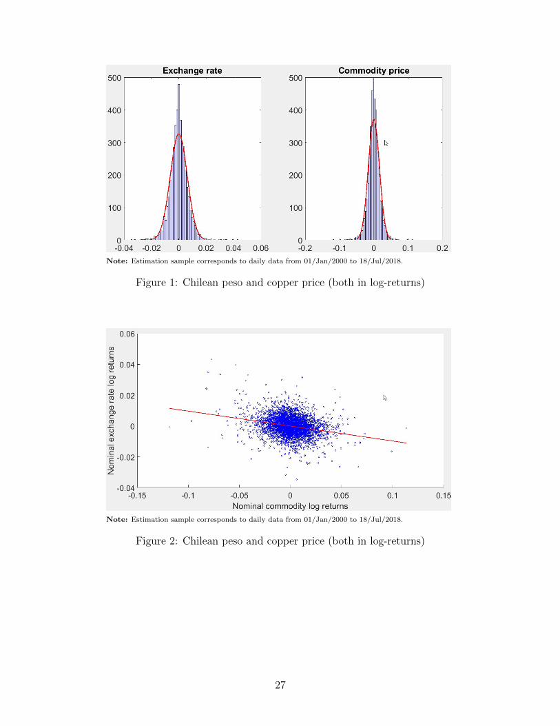
Note: Estimation sample corresponds to daily data from 01/Jan/2000 to 18/Jul/2018.

Figure 1: Chilean peso and copper price (both in log-returns)

Note: Estimation sample corresponds to daily data from 01/Jan/2000 to 18/Jul/2018.

Figure 2: Chilean peso and copper price (both in log-returns)

27

Notes: (1) Asymtotic dependence indicator (ADI) plotted in blue in the left-

hand side axis. Shaded area corresponds to periods when the China economic

surprise index exhibit negative economic surprises. (2) Asymptotic depen-

dence computed using 1000 daily observations and 2.5% as the tail percentile

(25 observations over the threshold). (4) Estimation sample corresponds to

daily data from 01/Jan/2000 to 18/Jul/2018. (5) The China surprise index

corresponds to the Citigroup China Economic Surprise Index obtained from

Bloomberg.

Figure 3: Asymptotic dependence and China economic surprise index

28

Table 1: Commodity exporter economies

Note: This table reports the mean percentage value of exports for each of three periods: 2000-2005, 2006-2011, and

2012-2017 for each country. Each period corresponds to the average values within those years. Source: United Nations

Conference on Trade and Development (UNCTAD) website (https://unctadstat.unctad.org/EN/Index.html).

29

Table 2: Contemporaneous commodity prices vs. RW model without drift

Notes: (1) MSFE ratio between the commodity-based model (numerator) and a RW model (denom-

inator). (2) Base currency: USD. (3) Benchmark model: RW without drift. (4) Stat. corresponds

to the statistic of the Diebold-Mariano test. (5) Statistical significance: (*) p < 0.1, (**) p < 0.05,

(***) p < 0.01. (6) Columns correspond to the selected forecast horizons. (7) Perfect foresight infor-

mation. Realised observations of explanatory variable. (8) Sample: Daily data from 01/Jan/2000 to

18/Jul/2018.

30

Table 3: Contemporaneous commodity prices vs. RW model with drift

Notes: (1) MSFE ratio between the commodity-based model (numerator) and a RW model (denomi-

nator). (2) Base currency: USD. (3) Benchmark model: RW with drift. (4) Stat. corresponds to the

statistic of the Diebold-Mariano test. (5) Statistical significance: (*) p < 0.1, (**) p < 0.05, (***)

p < 0.01. (6) Columns correspond to the selected forecast horizons. (7) Perfect foresight informa-

tion. Realised observations of explanatory variable. (8) Sample: Daily data from 01/Jan/2000 to

18/Jul/2018.

31



nator). (2) Base currency: USD. (3) Benchmark model: RW without drift. (4) Stat. corresponds to the

statistic of the Clark-West test. (5) Statistical significance: (*) p < 0.1, (**) p < 0.05, (***) p < 0.01.

(6) Columns correspond to the selected forecast horizons. (7) Perfect foresight information. Realised

observations of explanatory variable. (8) Sample: Daily data from 01/Jan/2000 to 18/Jul/2018.

32




statistic of the Clark-West test. (5) Statistical significance: (*) p < 0.1, (**) p < 0.05, (***) p < 0.01.

(6) Columns correspond to the selected forecast horizons. (7) Perfect foresight information. Realised

observations of explanatory variable. (8) Sample: Daily data from 01/Jan/2000 to 18/Jul/2018.

33

Table 6: Contemporaneous commodity prices vs. RW model without drift, using Euro as a

base currency


inator). (2) Base currency: EUR. (3) Benchmark model: RW without drift. (4) Stat. corresponds




18/Jul/2018.

34

Table 7: Contemporaneous commodity prices vs. RW model without drift, using Pound

Sterling as a base currency


inator). (2) Base currency: GBP. (3) Benchmark model: RW without drift. (4) Stat. corresponds




18/Jul/2018.

35

Table 8: Contemporaneous commodity prices vs. RW model without drift, using exchange

returns orthogonal to VIX index


inator). (2) We obtain exchange rate returns orthogonal to the VIX index by running the following

regression per country: st = α0 + α1d(V IX) + νt, where st corresponds to the exchange rate log-

return, d(V IX) is the change in the VIX index, and α0 and α1 are coefficients to be estimated. We

interpret the error term of above regression (νt) as the exchange rate log-returns that are orthogonal

to changes in the VIX. (3) Base currency: USD. (4) Benchmark model: RW without drift. (5) Stat.

corresponds to the statistic of the Diebold-Mariano test. (6) Statistical significance: (*) p < 0.1, (**) p

< 0.05, (***) p < 0.01. (7) Columns correspond to the selected forecast horizons. (8) Perfect foresight

information. Realised observations of explanatory variable. (9) Sample: Daily data from 01/Jan/2000

to 18/Jul/2018.

36

Table 9: Lagged commodity prices vs. RW model without drift




(***) p < 0.01. (6) Columns correspond to the selected forecast horizons. (7) Lagged observations of

explanatory variable. (8) Sample: Daily data from 01/Jan/2000 to 18/Jul/2018.

37

Table 10: Lagged commodity prices vs. RW model with drift



statistic of the Diebold-Mariano test. (5) Statistical significance: (*) p < 0.1, (**) p < 0.05, (***) p <

0.01. (6) Columns correspond to the selected forecast horizons. (7) Lagged observations of explanatory

variable. (8) Sample: Daily data from 01/Jan/2000 to 18/Jul/2018.

38



inator). (2) Base currency: USD. (3) Benchmark model: RW without drift. (4) Stat. corresponds to

the statistic of the Diebold-Mariano test. (5) Statistical significance: (*) p < 0.1, (**) p < 0.05, (***)

p < 0.01. (6) Columns correspond to the selected forecast horizons. (7) Perfect foresight information.

Realised observations of explanatory variable. (8) Sample: Monthly data from Jan/2000 to Jun/2018.

39




statistic of the Diebold-Mariano test. (5) Statistical significance: (*) p < 0.1, (**) p < 0.05, (***) p

< 0.01. (6) Columns correspond to the selected forecast horizons. (7) Perfect foresight information.

Realised observations of explanatory variable. (8) Sample: Monthly data from Jan/2000 to Jun/2018.

40





(***) p < 0.01. (6) Columns correspond to the selected forecast horizons. (7) Lagged observations of

explanatory variable. (8) Sample: Monthly data from Jan/2000 to Jun/2018.

41




statistic of the Diebold-Mariano test. (5) Statistical significance: (*) p < 0.1, (**) p < 0.05, (***) p <

0.01. (6) Columns correspond to the selected forecast horizons. (7) Lagged observations of explanatory

variable. (8) Sample: Monthly data from Jan/2000 to Jun/2018.

42





p < 0.01. (6) Columns correspond to the selected forecast horizons. (7) Perfect foresight information.

Realised observations of explanatory variable. (8) Sample: Quarterly data from Jan/2000 to Jun/2018.

43





< 0.01. (6) Columns correspond to the selected forecast horizons. (7) Perfect foresight information.

Realised observations of explanatory variable. (8) Sample: Quarterly data from Jan/2000 to Jun/2018.

44





p < 0.01. (6) Columns correspond to the selected forecast horizons. (7) Lagged commodity prices as

the main explanatory variable. (8) Sample: Quarterly data from Jan/2000 to Jun/2018.

45





< 0.01. (6) Columns correspond to the selected forecast horizons. (7) Lagged commodity prices as the

main explanatory variable. (8) Sample: Quarterly data from Jan/2000 to Jun/2018.

46

Table 19: Hill index estimator

Notes: Note: Confidence Intervals at 95% level in parenthesis. Daily log-

returns, Jan-2000 to July-2018 (4270 observations approx.). Threshold cor-

responds to 2.5% of the data (107 obs. approx.).

47

Table 20: Tail index estimator of Dekkers et al. (1989)

Notes: Confidence Intervals at 95% level in parenthesis. Daily log-returns,

Jan-2000 to July-2018 (4270 observations approx.). Threshold corresponds

to 2.5% of the data (107 obs. approx.). Source: Author’s calculations.

Table 21: ADI using contemporaneous commodity returns

Note: Confidence Intervals in parenthesis at 95% level and obtained by bootstrap using 5000 re-

sampling iterations. Daily log-returns, Jan-2000 to July-2018 (4270 observations approx.). Threshold

corresponds to 2.5% of the data (107 obs. approx.). Case 1: NER appreciation (∇S) and increase in

comm. price (∆Pcomm). Case 2: NER depreciation (∆S) and reduction in comm. price. (∇Pcomm)

Case 3: ∇S and ∇Pcomm. Case 4: ∆S and ∆Pcomm.

48

Table 22: ADI using contemporaneous commodity returns and exchange rates orthogonal to

VIX





Case 3: ∇S and ∇Pcomm. Case 4: ∆S and ∆Pcomm. We obtain exchange rate returns orthogonal

to the VIX index by running the following regression per country: st = α0 +α1d(V IX) + νt, where st

corresponds to the exchange rate log-return, d(V IX) is the change in the VIX index, and α0 and α1

are coefficients to be estimated. We interpret the error term of above regression (νt) as the exchange

rate log-returns that are orthogonal to changes in the VIX.

Table 23: ADI using contemporaneous commodity returns and exchange rates with EUR as

a base currency





Case 3: ∇S and ∇Pcomm. Case 4: ∆S and ∆Pcomm. Euro as a base currency.

49

Table 24: ADI using contemporaneous commodity returns and exchange rates with GBP as

a base currency





Case 3: ∇S and ∇Pcomm. Case 4: ∆S and ∆Pcomm. Pound Sterling as a base currency.

Table 25: ADI using contemporaneous commodity returns and controlling for heteroskedas-

ticity in log-returns





Case 3: ∇S and ∇Pcomm. Case 4: ∆S and ∆Pcomm. Exchange rates and commodity returns

corresponds to the standardised residual obtained from a GARCH(1,1) where the conditional variance

is modelled as σ2t = ω + αu2t−1 + βσ2

t−1. ut corresponds to the residuals of the mean equation for

returns, and the standardised residuals are computed as εt = ut/σt.

50

Table 26: ADI using lagged commodity returns





Case 3: ∇S and ∇Pcomm. Case 4: ∆S and ∆Pcomm.

Table 27: ADI using contemporaneous commodity returns at different frequencies

Note: Asymptotic dependence index computed at different frequencies using log-returns from Jan-

2000 to July-2018. “−−” indicates no statistical significance at 5%. Case 1: NER appreciation (∇S)

and increase in comm. price (∆Pcomm). Case 2: NER depreciation (∆S) and reduction in comm.

price. (∇Pcomm) Case 3: ∇S and ∇Pcomm. Case 4: ∆S and ∆Pcomm.

51

Table 28: ADI using lagged commodity returns at different frequencies

Note: Asymptotic dependence index computed at different frequencies using log-returns from Jan-

2000 to July-2018. “−−” indicates no statistical significance at 5%. Case 1: NER appreciation (∇S)

and increase in comm. price (∆Pcomm). Case 2: NER depreciation (∆S) and reduction in comm.

price. (∇Pcomm) Case 3: ∇S and ∇Pcomm. Case 4: ∆S and ∆Pcomm.

52

Appendices

A World’s top oil producers

Table A.1: World’s top oil producers

2000 2005 2010 2015 2016

United States 9,058 8,327 9,691 15,139 14,829

Saudi Arabia 9,476 11,496 10,908 12,072 12,387

Russia 6,724 9,511 10,290 11,040 11,250

China 3,389 3,871 4,572 5,146 4,863

Canada 2,753 3,096 3,442 4,511 4,594

Iraq 2,582 1,889 2,398 4,039 4,443

Iran 3,765 4,239 4,243 3,485 4,364

United Arab Emirates 2,572 2,845 2,815 3,673 3,765

Brazil 1,534 2,038 2,723 3,183 3,240

Kuwait 2,201 2,672 2,449 2,880 2,991

Note: Data in thousand barrels per day are on a calendar day basis.

Source: U.S. Energy Information Administration (EIA).

53

asymptotic dependence and exchange rate forecasting

Documents