Asymptotic distribution theory for break point estimators

in models estimated via 2SLS1

Otilia Boldea

Tilburg University

Alastair R. Hall2

University of Manchester

and

Sanggohn Han

SAS Institute

June 6, 2011

1We are grateful for the comments of the participants at the World Congress of the Econometric

Society, Shanghai, 2010, and to an anonymous referee for valuable comments. The second author

acknowledges the support of the ESRC grant RES-062-23-1351.2Corresponding author. Economics, SoSS, University of Manchester, Manchester M13 9PL, UK.

Email: alastair.hall@manchester.ac.uk

Abstract

In this paper, we present a limiting distribution theory for the break point estimator in a linear

regression model with multiple structural breaks obtained by minimizing a Two Stage Least

Squares (2SLS) objective function. Our analysis covers both the case in which the reduced

form for the endogenous regressors is stable and the case in which it is unstable with multiple

structural breaks. For stable reduced forms, we present a limiting distribution theory under two

different scenarios: in the case where the parameter change is of fixed magnitude, it is shown that

the resulting distribution depends on the distribution of the data and is not of much practical

use for inference; in the case where the magnitude of the parameter change shrinks with the

sample size, it is shown that the resulting distribution can be used to construct approximate

large sample confidence intervals for the break points. For unstable reduced forms, we consider

the case where the magnitudes of the parameter changes in both the equation of interest and the

reduced forms shrink with the sample size at potentially different rates and not necessarily the

same locations in the sample. The resulting limiting distribution theory can be used to construct

approximate large sample confidence intervals for the break points. Its usefulness is illustrated

via an application to the New Keynesian Phillips curve.

JEL classification: C12, C13

Keywords: Structural Change, Multiple Break Points, Instrumental Variables Estimation.

1 Introduction

Econometric time series models are based on the assumption that the economic relationships,

or “structure”, in question are stable over time. However, with samples covering extended

periods, this assumption is always open to question and this has led to considerable interest

in the development of statistical methods for detecting structural instability.1 In designing

such methods, it is necessary to specify how the structure may change over time and a popular

specification is one in which the parameters of the model are subject to discrete shifts at unknown

points in the sample. This scenario can be motivated by the idea of policy regime changes.2

Within this type of setting, the main concern is to estimate economic relationships in the different

regimes and compare them. However, since not all policy changes may impact the economic

relationship of interest, an important precursor to this analysis is the identification of the points

in the sample, if any, at which the parameters change. This raises the issue of how to perform

inference about the location of the so-called “break points”, that is the points in the sample at

which the parameters change, and motivates the interest to obtain a limiting distribution theory

for break point estimators.3 It is the latter which is the focus of this paper.

There is a literature in time series on the limiting distribution of break point estimators for

estimation of changes in the mean of processes; see Picard (1985), Bhattacharya (1987), Yao

(1987), Bai (1994, 1997). A limiting distribution theory has also been presented in the context

of linear regression models estimated via Ordinary Least Squares (OLS). Bai (1997) considers

the case in which there is only one break. He presents two alternative limit theories for the

break point estimator. One assumes the magnitude of change between the regimes is fixed; the

resulting distribution theory for the break-point turns out to depend on the distribution of the

data. The other assumes the magnitude of the parameter change is shrinking with the sample

size4: this approach leads to practical methods for inference about the location of the break1See inter alia Andrews and Fair (1988), Ghysels and Hall (1990), Andrews (1993), Sowell (1996), Hall and

Sen (1999) as well as the other references below.2For example, Bai (1997) explores the impact of changes in monetary policy on the relationship between

the interest rate and the discount factor in the US, and Zhang, Osborn, and Kim (2008) explore the impact of

monetary policy changes on the Phillips curve.3The term “change point” is also used in the literature to denote the points in the sample at which the

parameter values change.4The assumption of shrinking breaks is a mathematical device designed to produce confidence intervals for the

break points whose asymptotic properties provide a reasonable approximation to finite sample behaviour when

1

point. Bai and Perron (1998) consider the case of multiple break points that are estimated

simultaneously. They present a limiting distribution theory for the break point estimators based

on the assumption that the parameter change is shrinking as the sample size increases; this can

be used by practitioners to perform inference about the location of the break points.

One maintained assumption in Bai’s (1997) and Bai and Perron’s (1998) analyses is that the

regressors are uncorrelated with the errors so that OLS is an appropriate method of estimation.

This is a leading case, of course, but there are also many cases in econometrics where the

regressors are correlated with the errors and so OLS yields inconsistent estimators. Once OLS

is rejected as inappropriate, an alternative method of estimation must be chosen. A natural

alternative is Instrumental Variables (IV). There are two common approaches to IV estimation

in econometrics: Generalized Method of Moments (GMM) and Two Stage Least Squares (2SLS).

While GMM has become very popular, Hall, Han, and Boldea (2011) show that it is not well

suited to break point estimation in this context. Specifically, they show that minimizing the sum

of partial GMM minimands over all partitions of the sample fails to yield consistent estimates of

the break point in leading cases of interest. In contrast, Hall, Han, and Boldea (2011) show that

minimizing the 2SLS minimand yields consistent estimators of the break points. Inspection of

their proofs indicates that the contrasting behaviours of these estimators stem from differences

in the construction of their associated objective functions. The GMM minimand is the square of

sums. This structure allows the opportunity for the effects of the misspecification associated with

the selection of the wrong break point to offset in the minimand and confound the estimation of

the break point. In contrast, the 2SLS minimand is a sum of squares and this construction offers

no scope for the effects of misspecification to offset. We thus follow the approach of Hall, Han,

and Boldea (2011) and consider the case in which the estimation of the regression parameters

and break points is performed by minimizing a 2SLS objective function.5 Hall, Han, and Boldea

(2011) establish the consistency of these 2SLS estimators, a limiting distribution theory for the

2SLS estimators of the regression parameters, propose a number of tests for parameter variation

and a methodology for estimating the number of break points. However, they do not consider

the breaks are of “moderate” size; see Bai and Perron (1998).5There is a considerable literature on the use of Instrumental Variables (IV) and 2SLS in linear models with

endogenous regressors in econometrics; see Christ (1994) or Hall (2005)[Chapter 1] for a historical review and

examples in which such endogeneity arises.

2

the distribution of the break point estimators.

In this paper, we derive the distribution of the break point estimators based on minimization

of the 2SLS objective function. As in Hall, Han, and Boldea (2011), our analysis covers both

the case in which the reduced form for the endogenous regressors is stable and the case in which

it is unstable with multiple structural breaks.6

For stable reduced forms, we present a limiting distribution theory under two different scenar-

ios regarding the magnitude of the parameter change between regimes. First, if the parameter

change is of fixed magnitude, the resulting distribution is shown to be the natural extension

of Bai’s (1997) result for OLS estimators and is consequently dependent on the distribution of

the data. Second, if the magnitude of the parameter change shrinks with the sample size, the

resulting distribution can be used to construct approximate large sample confidence intervals

for the break points. For unstable reduced forms, we consider the case where the magnitude of

the parameter changes in both the equation of interest and the reduced form shrink with the

sample size at potentially different rates and different locations for the structural equation and

reduced form. The resulting limiting distribution theory can be used to construct approximate

large sample confidence intervals for the break points. These intervals are illustrated illustrated

via an application to the New Keynesian Phillips curve.

An outline of the paper is as follows. Section 2 contains results for the stable reduced form

case. Section 3 presents the analysis for the unstable reduced form case and several break point

estimators obtained using the methodology described in Hall, Han, and Boldea (2011). Section

4 reports results from the empirical application. Section 5 offers some concluding remarks. The

mathematical appendix contains sketch proofs of the main results in the paper. Boldea, Hall,

and Han (2010) contains complete proofs of all results and also reports results from a small

simulation study that demonstrates the finite sample performance of the intervals; this paper is

available from the authors upon request.6Note that all breaks in a structural system of equations are either reflected in the structural equation of

interest, or in the reduced forms, or both; thus it is important to distinguish between stable and unstable reduced

forms.

3

2 Stable reduced form case

In this section, we present a limiting distribution theory for the break point estimator based on

minimization of the 2SLS objective function in the case where the reduced form is stable. Section

2.1 describes the model and summarizes certain preliminary results. Section 2.2 presents the

limiting distribution of the break point estimators in both the fixed-break and shrinking-break

cases.

2.1 Preliminaries

Consider the case in which the equation of interest is a linear regression model with m breaks,

that is

yt = x′tβ

0x,i + z′1,tβ

0z1,i + ut, i = 1, ..., m + 1, t = T 0

i−1 + 1, ..., T 0i (1)

where T 00 = 0 and T 0

m+1 = T . In this model, yt is the dependent variable, xt is a p1 × 1 vector

of explanatory variables, z1,t is a p2 × 1 vector of exogenous variables including the intercept,

and ut is a mean zero error. We define p = p1 + p2. Given that some regressors are endogenous,

it is plausible that (1) belongs to a system of structural equations and thus, for simplicity, we

refer to (1) as the “structural equation”. As is commonly assumed in the literature, we require

the break points to be asymptotically distinct.

Assumption 1. T 0i = [Tλ0

i ], where 0 < λ01 < ... < λ0

m < 1.7

Throughout our analysis, it is assumed that m, the number of breaks, is known but their

locations λ0i are not.

To implement 2SLS, it is necessary to specify the reduced form for xt. In this section, we

consider the case in which the reduced form is stable,

x′t = z′t∆0 + v′t (2)

where zt = (zt,1, zt,2, ..., zt,q)′ is a q × 1 vector of instruments that is uncorrelated with both

ut and vt, ∆0 = (δ1,0, δ2,0, ..., δp1,0) with dimension q × p1 and each δj,0 for j = 1, ..., p1 has

dimension q × 1. We assume that zt contains z1,t.

7[ · ] denotes the integer part of the quantity in the brackets.

4

Hall, Han, and Boldea (2011) (HHB hereafter) propose the following method for estimation

of the structural equation based on minimizing a 2SLS objective function. On the first stage,

the reduced form for xt is estimated via OLS using (2) and let xt denote the resulting predicted

value for xt, that is

x′t = zt

′∆T = zt′(

T∑

t=1

ztzt′)−1

T∑

t=1

ztxt′. (3)

In the second stage, the structural equation,

yt = x′

tβ∗x,i + z′1,tβ

∗z1,i + ut, i = 1, ..., m + 1; t = Ti−1 + 1, ..., Ti, (4)

is estimated via OLS for each possible m-partition of the sample, denoted by Tjmj=1 or

(T1, . . . , Tm). We assume:

Assumption 2. Equation (4) is estimated over all partitions (T1, ..., Tm) such that Ti − Ti−1 >

maxq − 1, εT for some ε > 0 and ε < infi(λ0i+1 − λ0

i ).

Assumption 2 requires that each segment considered in the minimization contains a positive

fraction of the sample asymptotically; in practice ε is chosen to be small in the hope that the

last part of the assumption is valid.

Letting β∗i = (β∗

x,i′, β∗

z1,i′)′, for a given m-partition, the estimates of β∗ = (β∗

1′, β∗

2′, ..., β∗

m+1′)′

are obtained by minimizing the sum of squared residuals

ST (T1, ..., Tm; β) =m+1∑

i=1

Ti∑

t=Ti−1+1

(yt − x′tβx,i − z′1,tβz1,i)2 (5)

with respect to β = (β1′, β2

′, ..., βm+1′)′. We denote these estimators by β(Tim

i=1). The

estimates of the break points, (T1, ..., Tm), are defined as

(T1, ..., Tm) = arg minT1,...,Tm

ST

(T1, ..., Tm; β(Tim

i=1))

(6)

where the minimization is taken over all possible partitions, (T1, ..., Tm). The 2SLS estimates

of the regression parameters, β ≡ β(Timi=1) = (β′

1, β′2, ..., β

′m+1)′, are the regression parameter

estimates associated with the estimated partition, Timi=1.

HHB focus on inference about the parameters β0 = (β01′, ..., β0

m+1′)′, where β0

i = (β0x,i

′, β0

z1,i′)′.

Specifically, they derive the limiting distributions of both β and also various tests for parameter

variation. However, to establish these results, they need to prove certain convergence results

5

regarding the break point estimators. These results are also relevant to our analysis of the limit-

ing distribution of the break point estimator in the fixed-break case, and so we summarize them

below in a lemma. To present these results, we must state certain additional assumptions.

Assumption 3. (i) ht = (ut, v′t)′ ⊗ zt is an array of real valued n × 1 random vectors (where

n = (p1 + 1)q) defined on the probability space (Ω,F , P ), VT = V ar[∑T

t=1 ht] is such that

diag[γ−1T,1, . . . , γ

−1T,n] = Γ−1

T is O(T−1) where ΓT is the n×n diagonal matrix with the eigenvalues

(γT,1, . . . , γT,n) of VT along the diagonal; (ii) E[ht,i] = 0 and, for some d > 2, ‖ht,i‖d < κ <

∞ for t = 1, 2, . . . and i = 1, 2, . . .n where ht,i is the ith element of ht; (iii) ht,i is near

epoch dependent with respect to gt such that ‖ht − E[ht|Gt+mt−m]‖2 ≤ νm with νm = O(m−1/2)

where Gt+mt−m is a sigma- algebra based on (gt−m, . . . , gt+m); (iv) gt is either φ-mixing of size

m−d/(2(d−1)) or α-mixing of size m−d/(d−2).

Assumption 4. rank Υ0 = p where Υ0 = [∆0, Π], Π′ = [Ip2 , 0p2×(q−p2)], Ia denotes the

a × a identity matrix and 0a×b is the a × b null matrix.8

Assumption 5. There exists an 0 < l0 < minT 0i , T − T 0

i such that for all l with l0 <

l ≤ minT 0i , T − T 0

i , the minimum eigenvalues of Ail = (1/l)∑T0

i +l

t=T0i +1

ztzt′ and of A∗

il =

(1/l)∑T0

i

t=T0i −l

ztzt′ are bounded away from zero in probability for all i = 1, ..., m + 1.

Assumption 6. T−1∑[Tr]

t=1 ztz′t

p→ QZZ(r) uniformly in r ∈ [0, 1] where QZZ(r) is positive

definite (thereafter pd) for any r > 0 and strictly increasing in r.

Assumption 3 allows substantial dependence and heterogeneity in (ut, v′t)′⊗zt but at the same

time imposes sufficient restrictions to deduce a Central Limit Theorem for T−1/2∑[Tr]

t=1 ht; see

Wooldridge and White (1988).9 This assumption also contains the restrictions that the implicit

population moment condition in 2SLS is valid - that is E[ztut] = 0 - and the conditional mean

of the reduced form is correctly specified. Assumption 4 implies the standard rank condition for

identification in IV estimation in the linear regression model10 because Assumptions 3(ii), 4 and

8Note that this notation is convenient for calculations involving the augmented matrix of projected endogenous

regressors and observed exogenous regressors in the second stage.9This rests on showing that under the stated conditions ht,Gt

−∞ is a mixingale of size -1/2 with constants

cT,j = nξ−1/2T,j max(1,‖bt,j‖r); see Wooldridge and White (1988).

10See e.g. Hall (2005)[p.35].

6

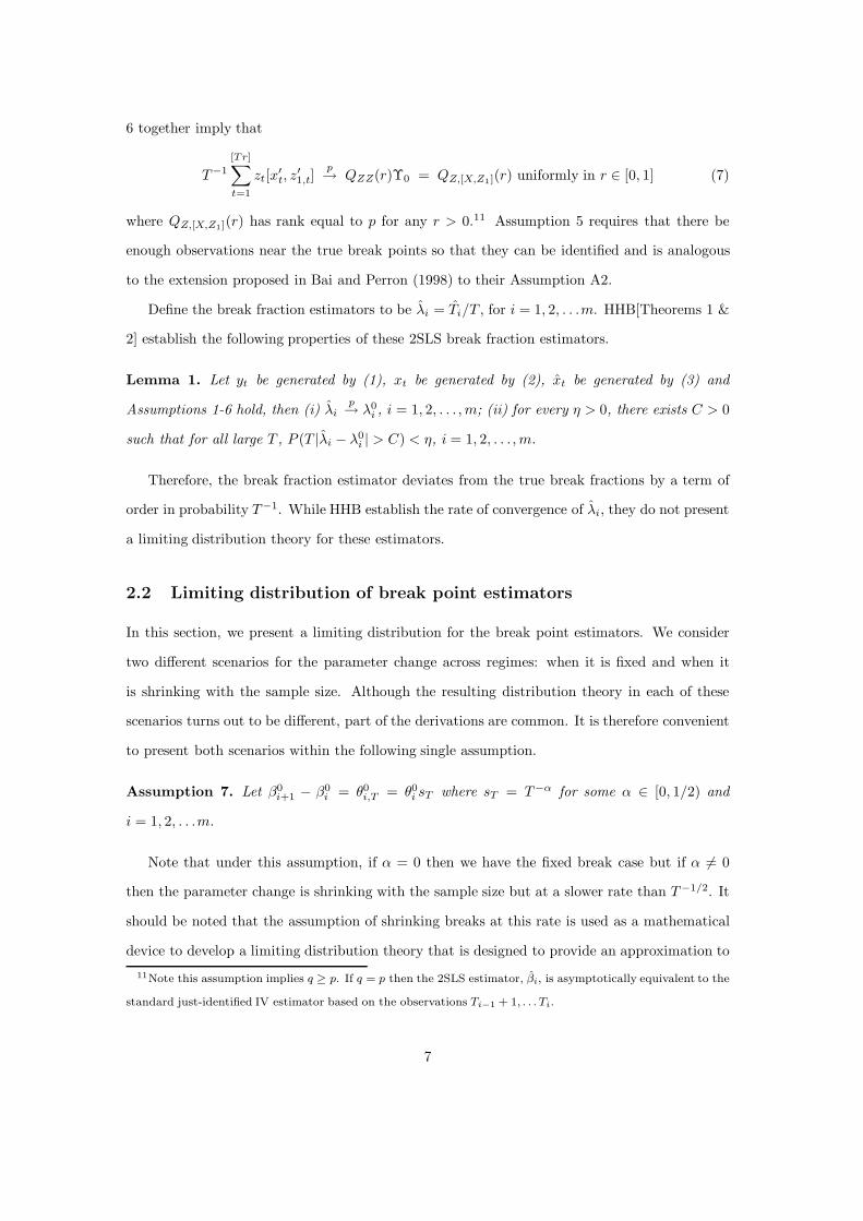
6 together imply that

T−1

[Tr]∑

t=1

zt[x′t, z

′1,t]

p→ QZZ(r)Υ0 = QZ,[X,Z1 ](r) uniformly in r ∈ [0, 1] (7)

where QZ,[X,Z1](r) has rank equal to p for any r > 0.11 Assumption 5 requires that there be

enough observations near the true break points so that they can be identified and is analogous

to the extension proposed in Bai and Perron (1998) to their Assumption A2.

Define the break fraction estimators to be λi = Ti/T , for i = 1, 2, . . .m. HHB[Theorems 1 &

2] establish the following properties of these 2SLS break fraction estimators.

Lemma 1. Let yt be generated by (1), xt be generated by (2), xt be generated by (3) and

Assumptions 1-6 hold, then (i) λip→ λ0

i , i = 1, 2, . . . , m; (ii) for every η > 0, there exists C > 0

such that for all large T , P (T |λi − λ0i | > C) < η, i = 1, 2, . . . , m.

Therefore, the break fraction estimator deviates from the true break fractions by a term of

order in probability T−1. While HHB establish the rate of convergence of λi, they do not present

a limiting distribution theory for these estimators.

2.2 Limiting distribution of break point estimators

In this section, we present a limiting distribution for the break point estimators. We consider

two different scenarios for the parameter change across regimes: when it is fixed and when it

is shrinking with the sample size. Although the resulting distribution theory in each of these

scenarios turns out to be different, part of the derivations are common. It is therefore convenient

to present both scenarios within the following single assumption.

Assumption 7. Let β0i+1 − β0

i = θ0i,T = θ0

i sT where sT = T−α for some α ∈ [0, 1/2) and

i = 1, 2, . . .m.

Note that under this assumption, if α = 0 then we have the fixed break case but if α 6= 0

then the parameter change is shrinking with the sample size but at a slower rate than T−1/2. It

should be noted that the assumption of shrinking breaks at this rate is used as a mathematical

device to develop a limiting distribution theory that is designed to provide an approximation to

11Note this assumption implies q ≥ p. If q = p then the 2SLS estimator, βi, is asymptotically equivalent to the

standard just-identified IV estimator based on the observations Ti−1 + 1, . . . Ti.

7

finite sample behaviour in models with moderate-sized changes in the parameters. The simula-

tion results in Section 4.1 provide guidance on the accuracy of this approximation for different

magnitudes of parameter change.

The derivation of the limiting distribution theory below is premised on the consistency and

the known rate of convergence of the break fraction estimators. These are already presented in

Lemma 1 for the fixed-break case. The corresponding results for the shrinking-break case are

presented in the following proposition.

Proposition 1. Let yt be generated by (1), xt be generated by (2), xt be generated by (3) and

Assumptions 1-7 (α 6= 0) hold, then (i) λip→ λ0

i , i = 1, 2, . . ., m; (ii) for every η > 0, there

exists C > 0 such that for all large T , P (T |λi − λ0i | > Cs−2

T ) < η, i = 1, 2, . . ., m.

Remark 1: Proposition 1(ii) states that the break point estimator converges to the true break

point at a rate equal to the inverse of the square of the rate at which the difference between

the regimes disappears. Note that this is the same rate of convergence as is exhibited by the

corresponding statistic in the case where xt and ut are uncorrelated and the model is estimated

by OLS; see Bai (1997)[Proposition 1].

We now turn to the issue of characterizing the limiting distribution of Ti. To achieve this

end, we first present the statistic that determines the large sample behaviour of the break point

estimator; see Proposition 2 below. The form of this statistic is the same for both the fixed-break

and the shrinking-break cases, but its large sample behaviour is different across the two cases.

We therefore consider the form of the limiting distribution in the fixed-break and shrinking-break

cases in turn.

From Lemma 1(ii) and Proposition 1(ii), it follows that in considering the limiting behaviour

of Timi=1 we can confine attention to possible break points within the following set B = ∪m

i=1Bi

where Bi = |Ti − T 0i | ≤ Cis

−2T , and Ci > 0 are constants.12

Proposition 2. Let yt be generated by (1), xt be generated by (2), xt be generated by (3) and

12See Han (2006) or an earlier version of this paper Hall, Han, and Boldea (2007) for a formal proof of this

assertion.

8

Assumptions 1-7 hold then:

Ti − T 0i = argminTi∈Bi

ΨT (Ti), for Ti 6= T 0i

0, for Ti = T 0i

(8)

where

ΨT (Ti) = (−1)I[Ti<T0i ]2θ0′

T,iΥ′0

Ti∨T0i∑

t=(Ti∧T0i )+1

zt

(ut + v′tβ

0x(t, T )

)

+ θ0′T,iΥ

′0

Ti∨T0i∑

t=(Ti∧T0i )+1

ztz′tΥ0θ

0T,i + op(1), uniformly in Bi,

β0x(t, T ) = β0

x,i for t = T 0i−1 + 1, T 0

i−1 + 2, . . . , T 0i and i = 1, 2, . . ., m + 1, a ∨ b = maxa, b,

a ∧ b = mina, b, and I[·] is an indicator variable that takes the value one if the event in the

square brackets occurs.

We now consider the implications of Proposition 2 for the limiting distribution of the break

point estimator in the two scenarios about the magnitude of the break.

(i) Fixed-break case:

If Assumption 7 holds with α = 0 then, without further restrictions, the limiting distribution of

the random variable on the right-hand side of (8) is intractable. A similar problem is encountered

by Bai (1997) in his analysis of the break points in models estimated by OLS. He circumvents

this problem by restricting attention to strictly stationary processes.13 We impose the same

restriction here.

Assumption 8. The process zt, ut, vt∞t=−∞ is strictly stationary.

To facilitate the presentation of the limiting distribution of Ti, we introduce a stochastic process

R∗i (s) on the set of integers that is defined as follows:

R∗i (s) =

R(i)1 (s) : s < 0

0 : s = 0

R(i)2 (s) : s > 0

13This approach is also pursued by Bhattacharya (1987), Picard (1985) and Yao (1987).

9

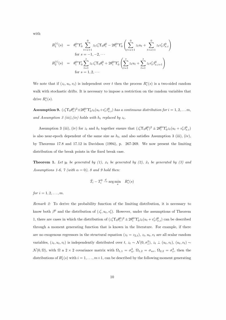
with

R(i)1 (s) = θ0′

i Υ′0

0∑

t=s+1

ztz′tΥ0θ

0i − 2θ0′

i Υ′0

(0∑

t=s+1

ztut +0∑

t=s+1

ztv′tβ

0x,i

)

for s = −1,−2, · · ·

R(i)2 (s) = θ0′

i Υ′0

s∑

t=1

ztz′tΥ0θ

0i + 2θ0′

i Υ′0

(s∑

t=1

ztut +s∑

t=1

ztv′tβ

0x,i+1

)

for s = 1, 2, · · ·

We note that if (zt, ut, vt) is independent over t then the process R∗i (s) is a two-sided random

walk with stochastic drifts. It is necessary to impose a restriction on the random variables that

drive R∗i (s).

Assumption 9. (z′tΥ0θ0i )2±2θ0′

i Υ′0zt(ut+v′tβ

0x,i) has a continuous distribution for i = 1, 2, . . .m,

and Assumption 3 (iii),(iv) holds with ht replaced by zt.

Assumption 3 (iii), (iv) for zt and ht together ensure that (z′tΥ0θ0i )2 ± 2θ0′

i Υ′0zt(ut + v′tβ

0x,i)

is also near-epoch dependent of the same size as ht, and also satisfies Assumption 3 (iii), (iv),

by Theorems 17.8 and 17.12 in Davidson (1994), p. 267-269. We now present the limiting

distribution of the break points in the fixed break case.

Theorem 1. Let yt be generated by (1), xt be generated by (2), xt be generated by (3) and

Assumptions 1-6, 7 (with α = 0), 8 and 9 hold then:

Ti − T 0i

d→ arg mins

R∗i (s)

for i = 1, 2, . . . , m.

Remark 2: To derive the probability function of the limiting distribution, it is necessary to

know both β0 and the distribution of (z′t, ut, v′t). However, under the assumptions of Theorem

1, there are cases in which the distribution of (z′tΥ0θ0i )2 ± 2θ0′

i Υ′0zt(ut + v′tβ

0x,i) can be described

through a moment generating function that is known in the literature. For example, if there

are no exogenous regressors in the structural equation (zt = z2,t), zt, ut, vt are all scalar random

variables, (zt, ut, vt) is independently distributed over t, zt ∼ N (0, σ2z), zt ⊥ (ut, vt), (ut, vt) ∼

N (0, Ω), with Ω a 2 × 2 covariance matrix with Ω1,1 = σ2u, Ω1,2 = σuv, Ω2,2 = σ2

v, then the

distributions of Ri1(s) with i = 1, . . . , m+1, can be described by the following moment generating

10

function:

Mi1(u) =

(%0

i σzϑi

)|s| × [ai(u)]−|s|/2 × exp

|s|

(ρ21 − ρ2

2,i)u2 + 2ρ1ρ2,iu

2ai(u)

where %0i = θ0

i ∆0 6= 0, ρ1 = µz/σz; ϑi =√

σ2z(%0

i )2 + σ2u + σ2

v(βi,0)2 + 2σuvβi,0; ρ2,i = µz%0i /ϑi;

ri = %0i σz/ϑi and ai(u) = [1 − (1 + riu)] × [1 + (1 − ri)u].14 The distribution of Ri

2(s) can be

described by Mi2(u), the same moment generating function above, but with βi,0 replaced with

β0i+1.

Remark 3: It is interesting to contrast our Proposition 2 with Bai’s (1997)[Proposition 2] in

which the limiting distribution of Ti is presented for the case in which m = 1, xt and ut are

uncorrelated and (1) is estimated via OLS. In the latter case, Bai (1997) shows that T1−T 01 −→d

arg maxs W ∗(s) where W ∗(s) has the same structure as R∗i (s) but its behaviour is driven by

b(xt, ut) = θ01′x′

txtθ01 ± 2xtut.

In contrast, the limiting distribution in Theorem 1 is driven by b(z′tΥ0, ut+v′tβ0x,i). Therefore the

limiting distribution in Theorem 1 is the same as would be obtained from Bai’s (1997)[Proposition

2] if yt is regressed on E[xt|zt] and z1,t using OLS.

Remark 4: The form of the limiting distribution of Ti is governed by R∗i (.). Given the assump-

tions of Theorem 1, the form of R∗i (.) only depends on i through θ0

i and β0x,i. In fact, the generic

nature of this form follows from Assumptions 1, 3 and 9, implying that Ti and Tj are asymptot-

ically independent for i 6= j.

In view of Remark 2, without further assumptions, the limiting distribution in Theorem 1 is not

useful for inference in general because of its dependence on unknowns. Therefore, we now turn

to an alternative framework that does yield practical methods of inference about the break points.

14This result, along with details about the distribution functions and their numerical computation, can be found

in Craig (1936). If we further assume that, for some regime, %0i = 1 and zt, respectively (ut + vtβ0

i ) are standard

normal variables, then in that regime, z2t − zt(ut + vtβ0

x,i) is the sum of a χ21 variable and an independently

distributed random variable with distribution function K0(u)/π, where K0(·) is the Bessel function of the second

kind of a purely imaginary argument of order zero - see e.g. Craig (1936), p. 1. Thus, the moment generating

function of Ri1(s) simplifies to Mi

1(u) = [√

2ai(u)]−|s|/2, with ri = 1/√

2.

11

(ii) Shrinking-break case:

Impose Assumption 7 with α 6= 0, as well as:

Assumption 10. T−1∑T0

i−1+[rT ]

t=T0i−1+1

ztz′t

p→ rQi, uniformly in r ∈ (0, λ0i − λ0

i−1], where Qi is a pd

matrix of constants.

Assumption 11. For regime i, i = 1, 2, . . .m, V ar [ht] = Vi, a n × n pd matrix of constants.

Assumption 10 allows the behaviour of the instrument cross product matrix to vary across

regimes, but it is more restrictive than Assumption 6. Assumption 11 restricts the error pro-

cesses to have constant second moments within regime but allows these moments to vary across

regimes. Both these assumptions are similar to their OLS counterparts - see e.g. Bai (1997)

and ensure that enough homogeneity is preserved such that the break-point estimators have a

pivotal asymptotic distribution; this is described below.

Theorem 2. Under Assumptions 1-5, 7 (with α 6= 0), 10 and 11, we have:

(θ0′i,T Υ′

0QiΥ0θ0i,T )2

θ0′i,T Υ′

0ΦiΥ0θ0i,T

(Ti − T 0i ) d→ arg min

cZi(c)

where

ξi =θ0′i Υ′

0Qi+1Υ0θ0i

θ0′i Υ′

0QiΥ0θ0i

, φi =θ0′i Υ′

0Φi+1Υ0θ0i

θ0′i Υ′

0ΦiΥ0θ0i

, Φi = CiViC′i, Ci = ν′

i ⊗ Iq, ν′i = [1 β0

x,i′]

Zi(c) =

|c|/2 − W(i)1 (−c) : c ≤ 0

ξic/2 −√

φiW(i)2 (c) : c > 0

, for i = 1, 2, . . .m + 1

β0x is the limiting common value of β0

x,i under Assumption 7 and W(i)j (c), j = 1, 2, for each

i, are two independent Brownian motion processes defined on [0,∞), starting at the origin when

c = 0, and W (i)j (c)2

j=1 is independent of W (k)j (c)2

j=1 for all k 6= i.

Remark 5: It is interesting to compare Theorem 2 with Bai’s (1997) Proposition 3, in which the

corresponding distribution is presented for m = 1 in the case where xt and ut are uncorrelated and

the model is estimated by OLS. The two limiting distributions have the same generic structure

but the definitions of ξ1, φ1, and Φ1 are different as is the scaling factor of k − k0. Inspection

reveals that the result in Theorem 2 is equivalent to what would be obtained from applying Bai’s

(1997) result to the case in which yt is regressed on E[xt|zt] and z1,t with error ut + v′tβ0x,i.

12

Remark 6: The density of arg minc Z(c) is characterized by Bai (1997) and he notes it is sym-

metric only if ξi = 1 and φi = 1. It is possible to identify in our setting one special case in which

ξi = φi = 1, that is where Vi+1 = Vi = V , Qi+1 = Qi = Q.

The distributional result in Theorem 2 can be used to construct confidence intervals for T 0i .

To this end, denote: θi = βi+1 − βi, Qi = (Ti − Ti−1)−1∑

i ztz′t, where

∑i denotes sum over

t = Ti−1+1, . . . , Ti, Vi = (Ti− Ti−1)−1∑

i hth′t, ht = [ut, v

′t]′⊗zt, wt = [x′

t, z′1,t]′, ut = yt−w′

tβi,

for t = Ti−1 + 1, . . . , Ti, i = 1, 2, . . .m, vt = (xt − ∆′Tzt), Ci = [1 β′

x,i] ⊗ Iq,

ξi =θ′iΥ

′T Qi+1ΥT θi

θ′iΥ′T QiΥT θi

, φi =θ′iΥ

′T Φi+1ΥT θi

θ′iΥ′T ΦiΥT θi

, Φi = CiViC′i

and ΥT = [∆T , Π].15 It then follows that(

Ti −[

a2

Hi

]− 1, Ti −

[a1

Hi

]+ 1

)(9)

is a 100(1−α) percent confidence interval for T 0i where [ · ] denotes the integer part of the term

in the brackets,

Hi =(θ′iΥ

′T QiΥT θi)2

θ′iΥ′T ΦiΥT θi

and a1 and a2 are respectively the α/2th and (1 − α/2)th quantiles for arg mins Z(s) which can

be calculated using equations (B.2) and (B.3) in Bai (1997). It is worth noting that even though

the asymptotic distribution may be symmetric, in general its finite sample approximation is not;

this is due to the fact that for each i, one estimates β0x by βx,i.

As in Bai (1997), assume instead that the conditional covariance of the error process is

constant across regimes.

Assumption 12. For regime i, i = 1, 2, . . .m, V ar[(ut, v′t)′|zt] = Ωi, a constant, pd matrix.

Then the asymptotic distribution simplifies.

Corollary 1. Under Assumptions 1-5, 7 (with α 6= 0), 10 and 12, Theorem 2 becomes:

θ0′i,T Υ′

0QiΥ0θ0i,T

ν′iΩiνi

(Ti − T 0i ) d→ arg min

cZi(c), for i = 1, 2, . . . , m.

Corollary 1 can be used to construct confidence intervals by consistently estimating Ωi via

Ωi = T−1/2(Ti − Ti−1)−1∑

i btb′t, bt = [ut, v

′t]′, where ut, vt and all the other relevant estimating

quantities are defined as for (9).

15Note that ΥTp→ Υ0 by the properties of OLS estimators, while ξi

p→ ξi, φip→ φi and Φi

p→ Φi because

Qip→ Qi and βi

p→ β0i , see derivations in Mathematical Appendix, Proof of Proposition 2, p. 33-34.

13

Remark 7: Boldea, Hall, and Han (2010) report simulation evidence for designs with one and

two breaks in the structural equation. This evidence suggests the intervals presented above

have approximately correct coverage in the sample sizes encountered in macroeconomics for

moderate-sized shifts in the parameters.

3 Unstable reduced form case

In this section, we present a limiting distribution theory for the break point estimator based on

minimization of the 2SLS objective function in the case where the reduced form is unstable. To

motivate the results presented, it is necessary to briefly summarize certain results in HHB.

For the unstable reduced form case, HHB propose a methodology for estimation of the break

points in which the break points are identified in the reduced form first and then, conditional on

these, the structural equation is estimated via 2SLS and analyzed for the presence of breaks using

a strategy based on partitioning the sample into sub-samples within which the reduced form is

stable.16 The basic idea is to divide the break points in the structural equation into two types:

(i) breaks that occur in the structural equation but not in the reduced form; (ii) breaks that

occur simultaneously in both the structural equation and reduced form. HHB’s methodology

estimates the number and location of the breaks in (i) and (ii) separately in the following two

steps.

• Step 1: for each sub-sample, the number of breaks in the structural equation are estimated

and their locations determined using 2SLS-based methods that assume a stable reduced

form.

• Step 2: for each break point in the reduced form in turn, a Wald statistic is used to test

if this break point is also present in the structural equation. If the evidence suggests the

break point is common then the location of the break point in question can be re-estimated

from the structural equation.17

The number and location of the breaks in the structural equation is then deduced by combining16This partitioning is crucial for obtaining pivotal statistics and confidence intervals for the break estimators

in the structural equation of interest.17There are two options at this point. In addition to the option given in the text, inference about the break

point can be based on the reduced form estimation.

14

the results from Steps 1 and 2. Within this methodology, two scenarios naturally arise for break

point estimators.

• Scenario 1: Step 1 involves a scenario in which break point estimators that only pertain to

the structural equation are obtained by minimizing a 2SLS criterion that assumes a stable

reduced form over sub-samples with potentially random end-points.

• Scenario 2: Step 2 involves a scenario in which a single break point is estimated by min-

imizing a 2SLS criterion that assumes an unstable reduced form over sub-samples with

potentially random end-points and with the break points in the reduced form estimated

(consistently) a priori and imposed in the construction of xt.

In this section, we present a distribution theory for both scenarios. To that end, note that

HHB develop their analysis under the assumption that the breaks in the reduced form are

fixed and π = π0 + Op(T−1). As part of this analysis, they establish that the consistency

and convergence rate results in Lemma 1 extend to the unstable reduced form case. However,

the previous section demonstrates that a shrinking-break framework is more fruitful for the

development of practical methods of inference. Therefore, we adopt the same framework here

and so assume shrinking-breaks in both the structural equation and the reduced form. As part of

our analysis, we establish the consistency and rate of convergence for the break point estimator

within this framework.

Section 3.1 describes the model and summarizes certain preliminary results. Section 3.2

presents the limiting distribution of the break point estimators.

3.1 Preliminaries

We now consider the case in which the reduced form for xt is:

x′

t = z′

t∆(i)0 + v

′

t, i = 1, 2, . . . , h + 1, t = T ∗i−1 + 1, . . . , T ∗

i (10)

where T ∗0 = 0 and T ∗

h+1 = T . The points T ∗i are assumed to be generated as follows.

Assumption 13. T ∗i = [Tπ0

i ], where 0 < π01 < . . . < π0

h < 1.

Thus, as with the structural equation, the breaks in the reduced form are assumed to be

asymptotically distinct. Note that the break fractions π0i may or may not coincide with λ0

i.

15

Throughout our analysis, it is assumed that h, the number of breaks, is known but their locations

π0i are not. Let π0 = [π0

1, π02, . . . , π

0h]′. Also note that (10) can be re-written as follows

x′

t = zt(π0)′Θ0 + v

′

t, t = 1, 2, . . . , T (11)

where Θ0 = [∆(1)′

0 , ∆(2)′

0 , . . . , ∆(h+1)′

0 ]′, zt(π0) = ι(t, T ) ⊗ zt, ι(t, T ) is a (h + 1) × 1 vector with

first element It/T ∈ (0, π01], h+1th element It/T ∈ (π0

h, 1], kth element It/T ∈ (π0k−1, π

0k]

for k = 1, 2, . . . , h and I· is an indicator variable that takes the value one if the event in the

curly brackets occurs.

Within our analysis, it is assumed that π0 is estimated prior to estimation of the structural

equation in (1). For our analysis to go through, the estimated break fractions in the reduced

form must satisfy certain conditions that are detailed below. Once the instability of the reduced

form is incorporated into xt, the 2SLS estimation is implemented in the fashion described in the

preamble to Section 3. However, the presence of this additional source of instability means that

it is also necessary to modify Assumption 2.

Assumption 14. The minimization in (6) is over all partitions (T1, ..., Tm) such that Ti−Ti−1 >

maxq − 1, εT for some ε > 0 and ε < infi(λ0i+1 − λ0

i ) and ε < infj(π0j+1 − π0

j ).

As noted in the preamble, our analysis is premised on shrinking breaks. Thus, in addition to

Assumption 7 with α 6= 0, we impose the following.

Assumption 15. ∆(i+1)0 − ∆(i)

0 = δ0i,T = δ0

i s∗T where s∗T = T−ρ, ρ ∈ (0, 0.5).

Note that like Asssumption 7, Assumption 15 implies the breaks are shrinking at a rate slower

than T−1/2. It is also worth pointing out that our analysis does not require any relationship

between α and ρ.

Let ΘT be the OLS estimator of Θ0 from the model

x′t = zt(π)′Θ0 + error t = 1, 2, · · · , T (12)

where zt(π) is defined analogously to zt(π0), and now define xt to be

x′t = zt(π)′ΘT = zt(π)′

T∑

t=1

zt(π)zt(π)′−1T∑

t=1

zt(π)x′t (13)

In our analysis we maintain Assumptions 3, 5 and 6 but need to replace the identification

condition in Assumption 4 by the following condition.

16

Assumption 16. rankΥ0j = p where Υ0

j =[∆(j)

0 , Π], for j = 1, 2, · · · , h + 1 for Π defined

in Assumption 4.

Using a similar manipulation to (7), it can be shown that Assumption 16 implies that β0i is

identified. 18

3.2 Limiting distribution theory for break point estimators

Scenario 1:

Consider the case in which the j + 1th regime for the reduced form coincides with ` + 1 regimes

for the structural equation that is,

Assumption 17. π0j < λ0

k < λ0k+1 < . . . < λ0

k+` < π0j+1, for some k and ` such that k + ` ≤ m.

Notice that Assumption 17 does not preclude the possibility that either λ0k−1 = π0

j and/or

λ0k+`+1 = π0

j+1, but refers to λ0k, . . . , λ0

k+` as indexing breaks that only pertain to the structural

equation of interest.

Let πj and πj+1 be the estimators of the π0j and π0

j+1. We consider the estimators of λ0i k+`

i=k

based on the sub-sample t = [T πj] + 1, . . . , [T πj+1] that is, λi = Ti/T where

(Tk, ..., Tk+`) = arg minTk,...,Tk+`

S(j)T

(Tk, ..., Tk+`; β(Tik+`

i=k))

(14)

and

S(j)T (Tk, ..., Tk+`; β) =

Tk∑

t=[Tπj ]+1

(yt − x′tβx,k − z′1,tβz1,k)2

+k+∑

i=k+1

Ti∑

t=Ti−1+1

(yt − x′tβx,i − z′1,tβz1,i)2

+[Tπj+1 ]∑

t=Tk+`+1

(yt − x′tβx,k+`+1 − z′1,tβz1,k+`+1)2 (15)

18Notice this assumption implies q ≥ p. If q = p then βi can be interpreted as a GMM estimator. To illustrate,

suppose there are no breaks in the structural equation (m = 0) and one break in the reduced form at t = [πT ],

then the 2SLS estimator of the structural equation parameters, β say, is equal to the GMM estimator based

on E[zt(yt − w′

tβ)⊗ (It/T ≤ π, It/T > π)′]

= 0 with weighting matrix diag(Z′1Z1/T )−1, (Z′

2Z2/T )−1

where wt = [x′t, z

′1,t ]

′, Z1 is a [πT ] × q matrix with tth row z′t, and Z2 is a [(1 − π)T ] × q matrix with ith row

z′[πT ]+i

. This interpretation can be extended to structural equations with breaks with appropriate modification

to reflect the sub-sample over which particular structural parameters are estimated.

17

where β(Tik+`i=k) denote the 2SLS estimators obtained by minimizing S

(j)T for the corresponding

partition of t = [T πj] + 1, . . . , [T πj+1].

The following proposition establishes the consistency and convergence rate of λi, for i =

k, k + 1, . . .k + `.

Proposition 3. Let yt be generated by (1), xt be generated by (2), xt be generated by (13) and

λi = Ti/T with Ti defined in (14). If Assumptions 1-5, 7 (with α 6= 0), 10, 13-17 hold, then for

i = k, k + 1, . . .k + ` we have: (i) λip→ λ0

i ; (ii) for every η > 0, there exists C > 0 such that for

all large T , P (T |λi − λ0i | > Cs−2

T ) < η.

Remark 8: A comparison of Propositions 1 and 3 indicates that consistency and the rate of

convergence are the same irrespective of whether the sample end-points are fixed or estimated

breaks from the reduced forms.

Remark 9: While Proposition 3 holds irrespective of whether λ0k−1 = π0

j and/or λ0k+`+1 = π0

j+1,

we note that if either of these conditions holds then it does impact on the limiting behaviour of

certain statistics considered in the proof of the proposition.19

Theorem 3. Let yt be generated by (1), xt be generated by (2), xt be generated by (13) and

λi = Ti/T with Ti defined in (14). If Assumptions 1-5, 7 (with α 6= 0), 10-11, 13-17 hold, then

for i = k, k + 1, . . .k + ` we have:

(θ0′i,T Υ′

0 QiΥ0θ0i,T )2

θ0′i,T Υ′

0 ΦiΥ0θ0i,T

(Ti − T 0i ) d→ arg min

cZi(c)

where

ξi =θ0′i Υ′

0Qi+1Υ0θ0i

θ0′i Υ′

0QiΥ0θ0i

, φi =θ0′i Υ′

0 Φi+1Υ0θ0i

θ0′i Υ′

0ΦiΥ0θ0i

,

Υ0 is the common limiting value of Υ0j under Assumption 15, Φi is defined as in Theorem 2

and Zi(c) is defined as in Theorem 2 but with the ξi and φi stated here.

Remark 10: A comparison of the limiting distributions in Theorems 2 and 3 reveals that they

are qualitatively the same. Thus, under the assumptions stated, the random end-points of the

estimation sub-sample do not impact on the limiting distribution of the break point estimator.19For brevity, we only present in the appendix a proof for the case in which λ0

k−1 6= π0j and λ0

k+`+1 6= π0j+1 .

A supplemental appendix (available from the authors upon request) contains the proof for the case in which

λ0k−1 = π0

j and/or λ0k+`+1 = π0

j+1 .

18

The distributional result in Theorem 3 can be used to construct confidence intervals for T 0i . To

this end, we introduce the following definitions: θi = βi+1−βi, Qi = (Ti−Ti−1)−1∑

i ztz′t, where

∑k denotes sum over t = [πjT ] + 1, [πjT ] + 2, . . . , Tk,

∑i denotes sum over t = Ti−1 + 1, Ti−1 +

2, . . . , Ti, for i=k + 1, . . .k + `,∑

k+`+1 denotes sum over t = Tk+` + 1, Tk+` + 2, . . . , [πj+1T ],

Ci = [1 β′x,i], Vi = (Ti − Ti−1)−1

∑i hth

′t, ht = [ut, v

′t]′ ⊗ zt, wt = [x′

t, z′1,t]

′, ut = yt − w′tβk,

for t = [πjT ] + 1, [πjT ] + 2, . . . , Tk+1, ut = yt − w′tβi for t = Ti−1 + 1, Ti−1 + 2, . . . , Ti and

i = k + 1, . . .k + `, ut = yt − w′tβk+`+1 for t = Tk+` + 1, Tk+` + 2, . . . , [πj+1T ], vt = (xt − ∆′

jzt),

∆j is the estimator of ∆(j)0 from (13),

ξi =θ′iΥ

′j+1Qi+1Υj+1θi

θ′iΥ′j+1QiΥj+1θi

, φi =θ′iΥ

′j+1Φi+1Υj+1θi

θ′iΥ′j+1ΦiΥj+1θi

, Φi = CiViC′i,

and Υj+1 = [∆j+1, Π].20 It then follows that(

Ti −[

a2

Hi

]− 1, Ti −

[a1

Hi

]+ 1

)(16)

is a 100(1−α) percent confidence interval for T 0i where [ · ] denotes the integer part of the term

in the brackets,

Hi =(θ′iΥ

′j+1QiΥj+1θi)2

θ′iΥ′j+1ΦiΥj+1θi

and a1 and a2 are defined as in (9).

Similarly to the stable reduced form case, if we impose constant conditional second moments

within regimes, the asymptotic distribution in Theorem 3 simplifies.

Corollary 2. Replace Assumption 11 with 12 in Theorem 3 and recall ν′i = [1 β0

x,i′]. Then

θ0′i,T Υ′

0 QiΥ0θ0i,T

ν′iΩiνi

(Ti − T 0i ) d→ arg min

cZi(c)

Corollary 2 can be used in a similar fashion to Corollary 1 to construct confidence intervals by

consistently estimating Ωi via Ωi, where all the other relevant estimating quantities are defined

as for the confidence interval above.

Scenario 2:

Consider the case in which20The estimating quantities are consistent for their true values, because under Assumptions 3, 10, 13-16,

∆jp→ ∆

(j)0 by e.g. Bai and Perron (1998) or Qu and Perron (2007), while Qi

p→ Qi and βip→ β0

i from

Mathematical Appendix, Proof of Theorem 3, p. 41.

19

Assumption 18. π0j−1 ≤ λ0

k−1 < π0j = λ0

k < λ0k+1 ≤ π0

j+1 for some j and k.21

Let πj be the estimator of π0j obtained from the reduced form, and λk−1, λk+1 be estimators

of λ0k−1, λ0

k+1 obtained via the method described in Scenario 1 above.

We consider the estimators of λ0k based on the sub-sample t = [T λk−1] + 1, . . . , [T λk+1] that

is, λk = Tk/T where

(Tk) = arg minTk

S(∗k)T (Tk; β(Tk)) (17)

and

S(∗k)T (Tk; β) =

Tk∑

t=[Tλk−1]+1

(yt− x′tβx,k−z′1,tβz1,k)2 +

[Tλk+1 ]∑

t=Tk+1

(yt− x′tβx,k+1−z′1,tβz1,k+1)2, (18)

where β(Tk) denote the 2SLS obtained by minimizing S(∗k)T for the given partition of t =

[T λk−1] + 1, . . . , [T λk+1].

Proposition 4. Let yt be generated by (1), xt be generated by (2), xt be generated by (13)

and λk = Tk/T with Tk defined in (17). If Assumptions 1-5, 7 (with α 6= 0), 10, 13-18 hold,

then we have: (i) λkp→ λ0

k; (ii) for every η > 0, there exists C > 0 such that for all large T ,

P (T |λk − λ0k| > Cs−2

T ) < η.

Remark 11: A comparison of Propositions 1, 3 and 4 indicates that consistency and the rate of

convergence properties are the same in all three cases covered.

Theorem 4. Let yt be generated by (1), xt be generated by (2), xt be generated by (13) and

λk = Tk/T with Tk defined in (17). If Assumptions 1-5, 7 (with α 6= 0), 10, 11, 13-18 hold, then

we have:(θ0′

k,T Υ′0 QkΥ0θ

0k,T )2

θ0′k,T Υ′

0 ΦkΥ0θ0k,T

(Tk − T 0k ) d→ arg min

cZk(c)

where Zk(c), Υ0, ξk, and φk are defined as in Theorem 3.

Remark 12: A comparison of the distributions in Theorems 2, 3 and 4 reveals that the limiting

distributions are qualitatively the same.

21Note that this case can be extended to multiple common break points in the same fashion as in Section 3.2,

Scenario 1.

20

The distributional result in Theorem 4 can be used to construct a confidence interval for T 0k .

The form of this interval is essentially the same as implied by (16) but with Υi+1 replaced by

Υi in the denominators of ξi and φi, where i = k here.22 Similarly, the asymptotic distribution

simplifies for the case of conditional constant second moments within regimes.

Corollary 3. Replace Assumption 11 with 12 in Theorem 4. Then

θ0′i,T Υ′

0 QiΥ0θ0i,T

ν′iΩiνi

(Ti − T 0i ) d→ arg min

cZi(c)

This can be used in a similar fashion to Corollary 2 to construct confidence intervals.

Remark: 13: Boldea, Hall, and Han (2010) report simulation evidence for designs with: (i)

one break in both the structural equation and reduced form, but the breaks in each equation

are not coincident; (ii) two breaks in the structural equation, one of which is coincident with

the sole break in the reduced form. This evidence suggests the intervals presented above have

approximately correct coverage in the sample sizes encountered in macroeconomics for moderate-

sized shifts in the parameters.

4 Empirical application

In this section, we assess the stability of the New Keynesian Phillips curve (NKPC), as formulated

in Zhang, Osborn, and Kim (2008). This version of the NKPC is a linear model with regressors,

some of which are anticipated to be correlated with the error. One contribution of their study is

to raise the question of whether monetary policy changes have caused changes in the parameters

in the NKPC. To investigate this issue, Zhang, Osborn, and Kim (2008) estimate the NKPC

via Instrumental Variables and use informal methods to assess whether the parameters have

exhibited discrete changes at any points in the sample. However, they provide no theoretical

justification for their methods. As can be recognized from the description, the scenario above

fits our framework, and in the sub-section we re-investigate the stability of the NKPC using the

methods in HHB. Our results indicate that there is instability in the NKPC, and we use the

theory developed in Section 3 to provide confidence intervals for the break point.22Note that the estimators are consistent for their true values by a similar reasoning as before, and the Proof

of Theorem 4 in Boldea, Hall, and Han (2010).

21

The data is quarterly from the US, spanning 1969.1-2005.4. The definitions of the variables

are the same as theirs: inft is the annualized quarterly growth rate of the GDP deflator, ogt

is obtained from the estimates of potential GDP published by the Congressional Budget Office,

and infet+1|t is taken from the Michigan inflation expectations survey.23 With this notation, the

structural equation of interest is:

inft = c0 + αf infet+1|t + αbinft−1 + αogogt +

3∑

i=1

αi∆inft−i + ut (19)

where inft is inflation in (time) period t, infet+1|t denotes expected inflation in period t+1 given

information available in period t, ogt is the output gap in period t, ut is an unobserved error

term and θ = (c0, αf , αb, αog, α1, α2, α3)′ are unknown parameters. The variables infet+1|t and

ogt are anticipated to be correlated with the error ut, and so (19) is commonly estimated via

IV; e.g. see Zhang, Osborn, and Kim (2008) and the references therein.

Suitable instruments must be both uncorrelated with ut and correlated with infet+1|t and ogt.

In this context, the instrument vector zt commonly includes such variables as lagged values of

expected inflation, the output gap, the short-term interest rate, unemployment, money growth

rate and inflation.24 Hence, the reduced forms are:

infet+1|t = z′tδ1 + v1,t (20)

ogt = z′tδ2 + v2,t (21)

where:

z′t = [1, inft−1, ∆inft−1, ∆inft−2, ∆inft−3, infet|t−1, ogt−1, rt−1, µt−1, ut−1]

with µt, rt and ut denoting respectively the M2 growth rate, the three-month Treasury Bill rate

and the unemployment rate at time t.

Our sample comprises T = 148 observations. Consistent with the methodology proposed

in HHB, we first need to account for any instability in the reduced forms. Using equation by

equation the methods proposed in Bai and Perron’s (1998), we find two breaks in the reduced

form for infet+1|t, with estimated locations 1975:2 and 1980:4, and one break in the reduced

23While Zhang, Osborn, and Kim (2008) consider inflation expectations from different surveys as well, we focus

for brevity on the Michigan survey only.24See Zhang, Osborn, and Kim (2008) for evidence that such instruments are not weak in our context.

22

form for ogt, with estimated location 1975:1; the corresponding 95% confidence intervals are

[1974 : 4, 1975 : 3], [1980 : 3, 1981 : 4], and [1974 : 4, 1976 : 1] respectively.

Following HHB, we first test for additional breaks over the sub-sample [1981 : 1, 2005 : 4] for

which the reduced form is estimated to be stable, and this yields no evidence of any additional

breaks.25 Next, as proposed in HHB, we use Wald tests to test the structural equation over

[1969:1,1980:4] for a known break at 1975 : 1, 1975 : 2, and over [1975:2,2005:4] for a known

break at 1980 : 4. The Wald tests have p-values 0.0389, 0.0014, and 0.9184 respectively, indicating

that only the first (true) break is common to the structural equation and the reduced forms,

and that the NKPC has a break toward the end of 1974 or early 1975 but its precise location

is unclear. Therefore, we re-estimate the NKPC allowing for a single unknown break in the

structural equation, imposing the breaks in the reduced forms.26 The proposed methodology in

Section 3.2 indicates the break to be at 1974 : 4, with corresponding parameter estimates:

for 1969:1-1974:4

inft = −4.75(1.77)

+ 0.39(0.22)

infet+1|t + 1.58

(0.47)inft−1 + 0.32

(0.21)ogt − 1.48

(0.56)∆inft−1 − 1.16

(0.46)∆inft−2

− 0.42(0.25)

∆inft−3

for 1975:1-2005:4

inft = −0.84(0.27)

+ 0.51(0.10)

infet+1|t + 0.55

(0.08)inft−1 + 0.06

(0.05)ogt − 0.33

(0.07)∆inft−1 − 0.25

(0.08)∆inft−2

− 0.29(0.09)

∆inft−3

The coefficient on output gap is insignificant, a common finding in the literature, see e.g.

Gali and Gertler (1999). As Zhang, Osborn, and Kim (2008), we find that the forward looking

component of inflation has become more important in recent years.27

Based on the result in Theorem 4, the 99%, 95% and 90% confidence intervals are all estimated

to be [1974 : 3, 1975 : 1].28 It is interesting to compare our results on the breaks with those

obtained in Zhang, Osborn, and Kim (2008). They report evidence of a break in the NKPC in25See Boldea, Hall, and Han (2010) for further details.26According to HHB, we should also test in [1969:1,1975:1] and [1975:2,1980:4] for an unknown break, but both

the samples are too small for obtaining meaningful results.27Note that the backward looking coefficient estimate is not 0.55, but 0.55-0.33=0.22, thus much smaller than

the forward looking component.28Note that the confidence intervals do not coincide before employing the integer part operator as in equation

(9).

23

1974-1975 and also find evidence of break in 1980 : 4. However, their methods make no attempt

to distinguish breaks in a structural equation of interest from those coming from other parts

of the system that cause breaks in at least one reduced form. In contrast, our analysis does

distinguish between these two types of breaks and we find evidence of a break in NKPC only at

the end of 1974 with the break in 1980 being present only in one of the reduced forms. Thus

our results refute evidence for 1980 : 4 as a break in the NKPC beyond the implied change it

induces in the conditional mean of the expected inflation.

5 Concluding remarks

In this paper, we present a limiting distribution theory for the break point estimators in a linear

regression model with multiple breaks, estimated via Two Stage Least Squares under two different

scenarios: stable and unstable reduced forms. For stable reduced forms, we consider first the

case where the parameter change is of fixed magnitude; in this case the resulting distribution

depends on the distribution of the data and is not of much practical use for inference. Secondly,

we consider the case where the magnitude of the parameter change shrinks with the sample

size; in this case, the resulting distribution can be used to construct approximate large sample

confidence intervals for the break point.

Due to the failure of the fixed-shifts framework to deliver pivotal statistics that can be used

for the construction of approximate confidence intervals, in the unstable reduced form scenario

we focus on shrinking shifts. As pointed out in Hall, Han, and Boldea (2011), handling break

point estimators for the structural equation requires pre-estimating the breaks in the reduced

form. In this paper, we show that pre-partitioning the sample with break points estimated from

the reduced form instead of the true ones does not impact the limiting distribution of the break

points that are specific to the structural equation only. Using the latter break point estimators to

re-partition the sample into regions of only common breaks, we derive the limiting distribution of

a newly proposed estimator for the common break point. Both scenarios allow for the magnitude

of the breaks to differ across equations. These methods are illustrated via an application to the

New Keynesian Phillips curve.

Our results add to the literature on break point distributions. Previous contributions have

concentrated on level shifts in univariate time series models or on parameter shifts in linear

24

regression models estimated via OLS in which the regressors are uncorrelated with the errors.

Within our framework, the regressors of the linear regression model are allowed to be correlated

with the error and the shifts are allowed to be nearly weakly identified at different rates across

equations, encompassing a large number of applications in macroeconomics.

Mathematical Appendix

Due to space constraints, we present only sketch proofs of the main results here. Complete proofs

of all results can be found in Boldea, Hall, and Han (2010).

The proof of Proposition 1 rests on certain results that are presented together in Lemma A.1,

whose proof can be found in Boldea, Hall, and Han (2010).

(a) Lemma A.1:

If Assumptions 1-7 hold then for wt = [x′t, z

′1,t]′ we have: (i)

∑[Tr]t=1 wtut = Op(T 1/2) uniformly

in r ∈ [0, 1]; (ii)∑[Tr]

t=1 wtw′t = Op(T ) uniformly in r ∈ [0, 1].

(b) Proof of Proposition 1:

Part (i): The basic proof strategy is the same as that for Lemma 1 in HHB and follows in two

steps. First, since the 2SLS estimators minimize the error sum of squares in (5), it follows that

(1/T )T∑

t=1

u2t ≤ (1/T )

T∑

t=1

u2t (22)

where ut = yt − x′

tβx,j − z′1,tβz1,j denotes the estimated residuals for t ∈ [Tj−1 + 1, Tj] in the

second stage regression of 2SLS estimation procedure and ut = yt − x′

tβ0x,i − z′1,tβ

0z1,i denotes the

corresponding residuals evaluated at the true parameter value for t ∈ [T 0i−1 + 1, T 0

i ]; and second,

using dt = ut − ut = x′

t(βx,j − β0x,i)− z

′

1,t(βz1,j − β0z1,i) over t ∈ [Tj−1 + 1, Tj]∩ [T 0

i−1 + 1, T 0i ], it

follows that

T−1T∑

t=1

u2t = T−1

T∑

t=1

u2t + T−1

T∑

t=1

dt2 − 2T−1

T∑

t=1

utdt. (23)

Consistency is established by proving that if at least one of the estimated break fractions does

not converge in probability to a true break fraction then the results in (22)-(23) contradict each

other.

25

From Hall, Han, and Boldea (2009) equation (60) it follows thatT∑

t=1

utdt = U ′PW∗ (W ∗ − W 0)β0 + U ′PW∗ U − U ′(W ∗ − W 0)β0 (24)

where PS denotes the projection matrix of S, i.e. PS = S(S′S)−1S′ for any matrix S, W ∗ is the

diagonal partition of W at [T1, T2, . . . , Tm], W is the T × p matrix with tth row w′t = [x′

t, z′1,t],

W 0 is the diagonal partition of W at [T 01 , T 0

2 , . . . , T 0m], U = [u1, u2, . . . , uT ].

For ease of presentation, we assume m = 2 but the proof generalizes in a straightforward

manner. Using Lemma A.1 and Assumption 7, it follows that29

‖W ∗′(W ∗ − W 0)β0‖ ≤ ‖

T1∨T01∑

t=(T1∧T01 )+1

wtw′t(β

02 − β0

1 )‖ + ‖T2∨T0

2∑

t=(T2∧T02 )+1

wtw′t(β

03 − β0

2)‖

= Op(TsT ), (25)

‖U ′(W ∗ − W 0)β0‖ ≤ ‖T1∨T0

1∑

t=(T1∧T01 )+1

utw′t(β

02 − β0

1)‖ + ‖T2∨T0

2∑

t=(T2∧T02 )+1

utw′t(β

03 − β0

2 )‖

= Op(T 1/2sT ). (26)

From (24)-(26), it follows that∑T

t=1 utdt = Op(T 1/2sT ); notice that this holds irrespective of

the relationship between Ti and T 0i .

Now consider∑T

t=1 d2t . Repeating the steps in the proof of HHB[Lemma1(ii)], if one of the

break fraction estimators does not converge to the true value then∑T

t=1 d2t = Op(TsT ), hence

∑Tt=1 d2

t >>∑T

t=1 utdt.30. This implies that (22) and (23) contradict each other, establishing

the desired result.

Part (ii): Without loss of generality, we assume m = 2 and focus on T2. Using a similar logic

to HHB’s proof of their Theorem 2, it follows that the desired result is established if it can be

shown that for each η > 0, there exists C > 0 and ε > 0 such that for large T ,

P(min[ST (T1, T2) − ST (T1, T

02 )]/(T 0

2 − T2) < 0)

< η (27)

where the minimum is taken over Vε(C) = |T 0i − Ti| ≤ εT, i = 1, 2; T 0

2 − T2 > Cs−2T and

we have suppressed the dependence of the residual sum of squares on the regression parameter

estimators for ease of presentation. By similar logic to HHB, it can be shown that

ST (T1, T2) − ST (T1, T02 )

T 02 − T2

≥ N1 − N2 − N3 (28)

29The symbols ∨ and ∧ are defined in Proposition 2.30Here, the symbol ‘>>’ denotes ‘of a larger order in probability’.

26

where

N1 = (β∗3 − β∆)′

(W ′

∆W∆

T 02 − T2

)(β∗

3 − β∆)

N2 = (β∗3 − β∆)′

(W ′

∆W

T 02 − T2

)(W ′W

T

)−1(W ′W∆

T

)(β∗

3 − β∆)

N3 = (β∗2 − β∆)′

(W ′

∆W∆

T 02 − T2

)(β∗

2 − β∆)

where β∗2 is the 2SLS estimator of the regression parameter based on t = T1+1, . . . , T2, β∆ is the

2SLS estimator of the regression parameter based on t = T2+1, . . . , T 02 , β∗

3 is the 2SLS estimator

of the regression parameter based on t = T 02 +1, . . . , T , W∆ = [0p×T2, wT2+1, . . . , wT0

2, 0p×(T−T0

2 )]′

and W is the diagonal partition of W at [T1, T2].

Since (T 02 − T2)−1W ′

∆W = Op(1) for large enough C and T−1W ′W = Op(1) from Lemma

A.1(ii), it follows that ‖T−1W ′∆W‖ = εOp(1) and so N1 >> N2 for large T , small ε. To show

that N1 also dominates N3, we must consider the behaviour of β∗2 , β∆ and β∗

3 . It can be shown

that β∆ = β02+Op(T−1/2) for large C, β∗

3 = β03+Op(T−1/2) and β∗

2 = β02+Op(T−1/2)+εOp(sT ) =

β02 + εOp(sT ). Combining these results, it follows that N1 = Op(s2

T ), N3 = ε2Op(s2T ), and so

N1 >> N3 for small enough ε. Furthermore, (W ′∆W∆)/(T 0

2 − T2) has non-negative eigenvalues

by construction and, by Assumptions 3 - 5, they bounded away from zero for large C with large

probability. This implies that for small ε and large C and large T , (27) holds.

Proof of Proposition 2

We focus on the two break case; the proof generalizes in a straightforward fashion to m > 2. We

can equivalently define the break point estimators via

(T1, T2) = argmin(T1,T2)∈B [SSR(T1, T2) − SSR(T 01 , T 0

2 )] (29)

where SSR(T1, T2) denotes the residual sum of squares from the second-step regression in 2SLS

of the structural equation assuming breaks at (T1, T2).

Since the case Ti = T 0i , i = 1, 2 is trivial, we concentrate on Ti 6= T 0

i for at least one i = 1, 2.

Define βi = βi(T1, T2) and βi = βi(T 01 , T 0

2 ), for i = 1, 2.31 In Boldea, Hall, and Han (2010), we

31This involves an abuse of notation with respect to the definition of βi in Section 2.1 but the interpretation is

clear from the context.

27

show that T 1/2(βi − βi) = Op(T−1/2s−1T ), for i = 1, 2, 3, u.B. where u.B stands for “uniformly

in B”.

Now consider SSR(T1 , T2) − SSR(T 01 , T 0

2 ). Using ut(β) = ut + w′t[β0(t, T ) − β], we have

ut(β)2 = ut + 2[β0(t, T ) − β]′wtut + [β0(t, T ) − β]′wtw′t[β

0(t, T ) − β]

and so

SSR(T1, T2) − SSR(T 01 , T 0

2 ) =T∑

t=1

at + 2T∑

t=1

ct = A + 2C, say, (30)

where

at = [β(t, T ) − β(t, T )]′wtw′t[β0(t, T ) − β(t, T )] + [β0(t, T ) − β(t, T )], (31)

ct = [β(t, T ) − β(t, T )]′wtut, (32)

β(t, T ) = βi, for t ∈ [Ti−1 + 1, . . . , Ti], i = 1, 2, 3, T0 = 1, T3 = T,

β(t, T ) = βi, for t ∈ [T 0i−1 + 1, . . . , T 0

i ], i = 1, 2, 3, T 00 = 1, T 0

3 = T.

Define Bc ≡ [1, T ] \ (B1 ∪ B2). Then

A =∑

B1

at +∑

B2

at +∑

Bc

at (33)

where∑

Bidenotes sum over t ∈ Bi and

∑Bc denotes sum over t ∈ Bc. On Bc, we have

T 1/2[β(t, T ) − β(t, T )] = T 1/2[βi − βi] = Op(T−1/2s−1T ) = op(1). On Bi(i = 1, 2), one can show

that T 1/2[β(t, T ) − β(t, T )] = (−1)I[Ti<T0i ]T 1/2θ0

T,i + Op(1). Therefore, we have for i = 1, 2,

∑

Bi

at = θ0′T,iΥ

′0

Ti∨T0i∑

t=(Ti∧T0i )+1

ztz′tΥ0θ

0T,i + op(1), u.B (34)

In contrast, we have∑

Bc at = op(1), u.B, so:

A =2∑

i=1

θ0′

T,iΥ′0

Ti∨T0i∑

t=(Ti∧T0i )+1

ztz′tΥ0θ

0T,i

+ op(1), u.B (35)

By similar arguments, we have

C =2∑

i=1

(−1)I[Ti<T0

i ]θ0′T,iΥ

′0

Ti∨T0i∑

t=(Ti∧T0i )+1

zt[ut + v′tβ0x(t, T )]

+ op(1), u.B. (36)

The proof is completed by combining (35) and (36), and noting that by Assumption 3, the seg-

ments [(T1 ∧ T 01 ) + 1, T1 ∨ T 0

1 ] and [(T2 ∧ T 02 ) + 1, T2 ∨ T 0

2 ] are asymptotically independent.

28

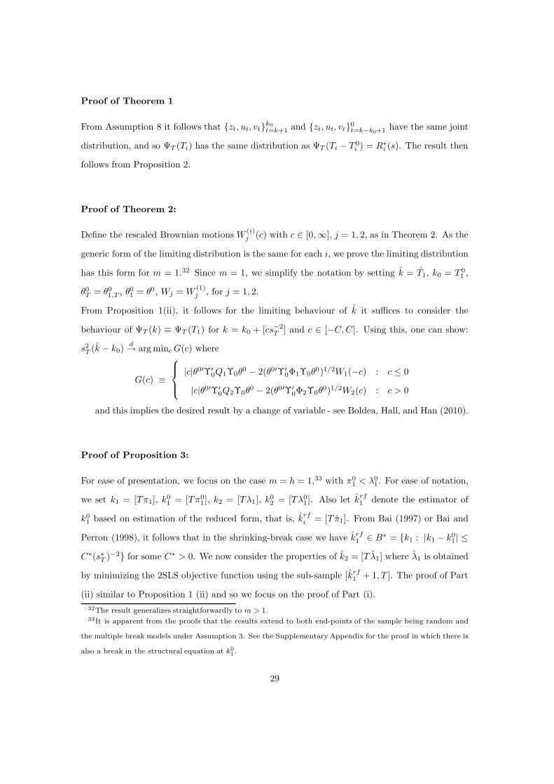
Proof of Theorem 1

From Assumption 8 it follows that zt, ut, vtk0t=k+1 and zt, ut, vt0

t=k−k0+1 have the same joint

distribution, and so ΨT (Ti) has the same distribution as ΨT (Ti − T 0i ) = R∗

i (s). The result then

follows from Proposition 2.

Proof of Theorem 2:

Define the rescaled Brownian motions W(i)j (c) with c ∈ [0,∞], j = 1, 2, as in Theorem 2. As the

generic form of the limiting distribution is the same for each i, we prove the limiting distribution

has this form for m = 1.32 Since m = 1, we simplify the notation by setting k = T1, k0 = T 01 ,

θ0T = θ0

1,T , θ01 = θ0, Wj = W

(1)j , for j = 1, 2.

From Proposition 1(ii), it follows for the limiting behaviour of k it suffices to consider the

behaviour of ΨT (k) ≡ ΨT (T1) for k = k0 + [cs−2T ] and c ∈ [−C, C]. Using this, one can show:

s2T (k − k0)

d→ arg minc G(c) where

G(c) ≡

|c|θ0′Υ′0Q1Υ0θ

0 − 2(θ0′Υ′0Φ1Υ0θ

0)1/2W1(−c) : c ≤ 0

|c|θ0′Υ′0Q2Υ0θ

0 − 2(θ0′Υ′0Φ2Υ0θ

0)1/2W2(c) : c > 0

and this implies the desired result by a change of variable - see Boldea, Hall, and Han (2010).

Proof of Proposition 3:

For ease of presentation, we focus on the case m = h = 1,33 with π01 < λ0

1. For ease of notation,

we set k1 = [Tπ1], k01 = [Tπ0

1], k2 = [Tλ1], k02 = [Tλ0

1]. Also let krf1 denote the estimator of

k01 based on estimation of the reduced form, that is, krf

i = [T π1]. From Bai (1997) or Bai and

Perron (1998), it follows that in the shrinking-break case we have krf1 ∈ B∗ = k1 : |k1 − k0

1| ≤

C∗(s∗T )−2 for some C∗ > 0. We now consider the properties of k2 = [T λ1] where λ1 is obtained

by minimizing the 2SLS objective function using the sub-sample [krf1 + 1, T ]. The proof of Part

(ii) similar to Proposition 1 (ii) and so we focus on the proof of Part (i).32The result generalizes straightforwardly to m > 1.33It is apparent from the proofs that the results extend to both end-points of the sample being random and

the multiple break models under Assumption 3. See the Supplementary Appendix for the proof in which there is

also a break in the structural equation at k01 .

29

Proof of Part (i): For ease of notation, set k1 = krf1 . By similar arguments to (24), we have

T∑

t=k1

utdt = U ′PW∗ (W ∗ − W 0)β0 + U ′PW∗ U − U ′(W ∗ − W 0)β0 (37)

where W ∗ is now a diagonal partition of W at k2, W = [wk1+1, wk1+2, . . . , wT ]′, W 0 is now the

diagonal partition of W at k02, U = [uk1+1, uk1+2, . . . , uT ].

To determine the order of the terms in (37), define δ(t, T ) = ∆0(t, T ) − ∆(t, T ), where

∆0(t, T ) = ∆01 It ≤ k0

1 + ∆02 It > k0

1, ∆(t, T ) = ∆1 It ≤ k1 + ∆2It > k1. Since

k1 ∈ B∗, it follows by standard arguments that ∆2 = ∆02+Op(T−1/2) and this property combined

with Assumption 15 yields

δ(t, T ) = Op(T−1/2) + O(s∗T )Ik1 ≤ k01, t ≤ k0

1 (38)

Using (38), it can be shown that34 W ∗′W ∗ = Op(T ), W ∗′U = Op(T 1/2) and U ′(W ∗ −

W 0)β0 = Op(T 1/2sT ). Hence,∑T

t=k1+1 utdt = Op(T 1/2sT ), and∑T

t=k1+1 d2t = Op(TsT ). The

result follows by similar arguments to the proof of Proposition 1 (i).

Proof of Theorem 3

Consider again m = h = 1. Define β1, β2, β1 and β2 to be the 2SLS estimators based on

t ∈ [k1 + 1, k2], t ∈ [k2 + 1, T ], t ∈ [k1 + 1, k02], respectively t ∈ [k0

2 + 1, T ]. To facilitate the proof,

consider the properties of these estimators. Note that from Proposition 3 (ii), it follows that we

need to consider only k2 ∈ B2 = k2 : |k2 − k02| < C2s

−2T . One can show that T 1/2(β1 − β1) =

Op(T−1/2s−1T ) u.B2, β2 = β0

2 + Op(T−1/2), and T 1/2(β2 − β2) = Op(T−1/2s−1T )u.B2.

With this background, we now consider the distribution of k2, where

k2 = argmink2∈B2 [SSR(k1, k2) − SSR(k1, k02)]

and SSR(k1, k2) denotes the residual sum of squares in interval [k1 + 1, T ] with partition at k2.

Obviously if k2 = k02 then the minimand is zero, and so we concentrate on the case in which

k2 6= k02.

Define β(t, T ) = β1It ≤ k2 + β2It > k2 and β(t, T ) = β1It ≤ k02 + β2It > k0

2.

One can show that T 1/2[β(t, T ) − β(t, T )] = Op(T−1/2s−1T ) + T 1/2sT θ0

1(−1)Ik2<k02 + Op(1).

34See Boldea, Hall, and Han (2010).

30

Let B2 = [k1 + 1, T ] \ [(k2 ∧ k02) + 1, k2 ∨ k0

2], then

SSR(k1, k2) − SSR(k1, k02) =

T∑

t=k1+1

at + 2T∑

t=k1+1

ct = A + 2C (39)

where at = T 1/2[β(t, T ) − β(t, T )]T−1wtw′t

T 1/2[β0(t, T ) − β(t, T )] + T 1/2[β0(t, T ) − β(t, T )]

,

and ct = T 1/2[β(t, T ) − β(t, T )]T−1/2wtut. By similar arguments to the proof of Theorem 2,

A = θ0′T,1Υ

0′2 Q2Υ0

2θ0T,1|k0

2 − k2| + op(1), u.B2,

and

C = (−1)Ik2<k02θ0′

T,1Υ0′2 T−1/2

k2∨k02∑

t=(k2∧k02)+1

zt[ut + v′tβ0x(t, T )] + op(1), u.B2.

Since the limit of A + 2C has the same basic structure as in Proposition 2, the rest of the proof

follows by similar arguments.

Proofs of Proposition 4 and Theorem 4

Consider the model with m = 2 and h = 1, with π01 = λ0

1, thus T ∗1 = T 0

1 in the notation

of Section 3.2. The key to the proof is to recognize that since the break-point estimator in the

reduced form T ∗1 is in a small neighborhood around T 0

1 , it has no impact on the asymptotic

properties of the second break-point estimator in the structural equation. Having recognized

this, the proofs of Proposition 4 and Theorem 4 follow in a similar manner to Proposition 3 and

Theorem 3 - see Boldea, Hall, and Han (2010).

31

References

Andrews, D. W. K. (1993). ‘Tests for parameter instability and structural change with unknown

change point’, Econometrica, 61: 821–856.

Andrews, D. W. K., and Fair, R. (1988). ‘Inference in econometric models with structural change’,

Review of Economic Studies, 55: 615–640.

Bai, J. (1994). ‘Least squares estimation of a shift in linear processes’, Journal of Time Series

Analysis, 15: 453–472.

(1997). ‘Estimation of a change point in multiple regression models’, Review of Economics

and Statistics, 79: 551–563.

Bai, J., and Perron, P. (1998). ‘Estimating and testing linear models with multiple structural

changes’, Econometrica, 66: 47–78.

Bhattacharya, P. K. (1987). ‘Maximum Likelihood estimation of a change-point in the distribu-

tion of independent random variables: general multiparameter case’, Journal of Multivariate

Analysis, 23: 183–208.

Boldea, O., Hall, A. R., and Han, S. (2010). ‘A distribution theory for change point estimators

in models estimated via 2SLS’, Discussion paper, Department of Economics, University of

Manchester, Manchester UK.

Christ, C. F. (1994). ‘The Cowles Commission’s contributions to econometrics at Chicago, 1939-

1955’, Journal of Economic Literature, 32: 30–59.

Craig, C. C. (1936). ‘On the frequency function of xy’, Annals of Mathematical Statistics, 7:

1–15.

Davidson, J. (1994). Stochastic Limit Theory. Oxford University Press, Oxford, UK.

Gali, J., and Gertler, M. (1999). ‘Inflation dynamics: a structural econometric analysis’, Journal

of Monetary Economics, 44: 195–222.

Ghysels, E., and Hall, A. R. (1990). ‘A test for structural stability of Euler condition parameters

estimated via the Generalized Method of Moments’, International Economic Review, 31: 355–

364.

32

Hall, A. R. (2005). Generalized Method of Moments. Oxford University Press, Oxford, U.K.

Hall, A. R., Han, S., and Boldea, O. (2007). ‘A distribution theory for change point estimators in

models estimated by Two Stage Least Squares’, Discussion paper, Department of Economics,

North Carolina State University, Raleigh, NC.

(2009). ‘Inference Regarding Multiple Structural Changes in Linear Models with En-

dogenous Regressors’, Discussion paper, Economics, School of Social Studies, University of

Manchester, Manchester, UK.

(2011). ‘Inference Regarding Multiple Structural Changes in Linear Models with En-

dogenous Regressors’, Journal of Econometrics, accepted for publication.

Hall, A. R., and Sen, A. (1999). ‘Structural stability testing in models estimated by Generalized

Method of Moments’, Journal of Business and Economic Statistics, 17: 335–348.

Han, S. (2006). ‘Inference regarding multiple structural changes in linear models estimated via

Instrumental Variables’, Ph.D. thesis, Department of Economics, North Carolina State Uni-

versity, Raleigh, NC.

Picard, D. (1985). ‘Testing and estimating change points in time series’, Journal of Applied

Probability, 20: 411–415.

Qu, Z., and Perron, P. (2007). ‘Estimating and testing structural changes in multivariate regres-

sions’, Econometrica, 75: 459–502.

Sowell, F. (1996). ‘Optimal tests of parameter variation in the Generalized Method of Moments

framework’, Econometrica, 64: 1085–1108.

Wooldridge, J., and White, H. (1988). ‘Some invariance principles and central limt theorems for

dependent heterogeneous processes’, Econometric Theory, 4: 210–230.

Yao, Y.-C. (1987). ‘Approximating the distribution of the ML estimate of the change point in a

sequence of independent r.v.’s’, Annals of Statistics, 4: 1321–1328.

Zhang, C., Osborn, D., and Kim, D. (2008). ‘The new Keynesian Phillips curve: from sticky

inflation to sticky prices’, Journal of Money, Credit and Banking, 40: 667–699.

33