Asymptotic Properties of Computationally

Efficient Alternative Estimators for a Class of

Multivariate Normal Models

Petruta C. Caragea 1,3

Department of Statistics, Iowa State University, 314 Snedecor Hall, Ames, IA,50011-1210

Richard L. Smith 2

Department of Statistics and Operations Research, University of North Carolina,Chapel Hill, NC 27599-3260

Abstract

Parameters of Gaussian multivariate models are often estimated using the maxi-mum likelihood approach. In spite of its merits, this methodology is not practicalwhen the sample size is very large, as, for example, in the case of massive geo-referenced data sets. In this paper, we study the asymptotic properties of the es-timators that minimize three alternatives to the likelihood function, designed toincrease the computational efficiency. This is achieved by applying the informationsandwich technique to expansions of the pseudo-likelihood functions as quadraticforms of independent normal random variables. Theoretical calculations are givenfor a first order autoregressive time series and then extended to a two-dimensionalautoregressive process on a lattice. We compare the efficiency of the three estimatorsto that of the maximum likelihood estimator as well as among themselves, usingnumerical calculations of the theoretical results and simulations.

Key words: Approximate likelihood. Massive Data Sets. ComputationalEfficiency. Statistical Efficiency Analysis. Spatial Statistics. AutoregressiveProcesses on a Lattice.

1 Supported in part by a SAMSI graduate studentship (NSF grant DMS-0112069)and by NSF grant DMS-0084375 while a graduate student at the University of NorthCarolina at Chapel Hill.2 Supported in part by NSF grant DMS-0084375.3 Corresponding author. Phone: +1 515 294 5582, Fax: +1 515 294 4040E-mail address: pcaragea@iastate.edu (P.C. Caragea)

Preprint submitted to Elsevier Science 12 May 2006

1 Introduction

Often times, it is assumed that modeling “geostatistical” processes withinthe realm of multivariate normal models is appropriate. There is by now asubstantial literature on the selection and estimation of models for spatialdata (see e.g. Cressie [10], Stein [22], Chiles and Delfiner [9], Banerjee et al.[3]). Many of the common geostatistical models may be expressed in the form

X ∼ N (µ,Σ(θ)) , (1)

with {Xi, i = 1, ..., N} the vector of observations with mean µ and N × Ncovariance matrix Σ(θ) (assumed of a known format), expressed in terms ofa finite-dimensional parameter vector θ. A simple example is the exponentialcovariance model, σij = θ1e

−dij/θ2 where σij represents the covariance betweenobservations Xi and Xj, dij is the physical distance between the two locations,and θ1 and θ2 are model parameters.

In such models, it is widely recognized that either the method of maximumlikelihood or the closely related technique of restricted maximum likelihood(Cressie [10], Stein [22]) are the best general methods of estimation. Maximumlikelihood is based on minimizing the negative log likelihood function which,modulo some constants, is of the form:

`(µ, θ) =1

2log |Σ(θ)|+ 1

2(Y − µ)T Σ(θ)−1(Y − µ). (2)

A disadvantage of likelihood-related techniques, however, is the computationalefficiency of the likelihood function. Evaluation of (2) requires calculating theinverse and determinant of a N × N matrix, which according to most com-monly used algorithms, requires O(N3) steps. Many modern data sets containthousands of observations, for which such computation is prohibitively timeconsuming. Therefore, there is some interest in finding approximations to thelikelihood function that are more efficient to compute, while trying not tosacrifice much statistical efficiency.

Several computationally efficient alternatives to maximum likelihood estima-tion have been explored in the literature. One such strategy was proposedby Vecchia [26] who computed approximate conditional densities along somesequence of arbitrarily ordered sampling points and ignoring long-range cor-relations. Recently Stein et. al [23] generalized Vecchia’s idea in a number ofways. They developed a variant of the method to approximate the restrictedlikelihood function in place of the likelihood function itself. They argued that,rather than evaluate conditional densities one observation at a time, it mightbe more efficient to do it in blocks.

2

Another approach to efficiently estimate semivariograms is explored by Cur-riero and Lele [11] who exploit the composite likelihood introduced by Lind-say [18] for the estimation of spatial hierarchical model parameters. The sameprinciples are also applied to modeling binary data in a subsequent paper byHeagerty and Lele [14]. The main idea proposed is to construct an approx-imate log-likelihood function by adding marginal log-likelihoods even whenthese components do not necessarily represent independent replicates.

For massive data sets, several efforts have been put into developing efficientinterpolation techniques that do not rely on using arbitrarily chosen localkriging neighborhoods (see Cressie [10]). Recent advancements in the fieldpropose approximations to the kriging equations by tapering the covariancematrix, as in Furrer et. al [12] which may have the disadvantage of ignoringlong range correlations. Other suggestions include iterative methods to solvelinear systems such as conjugated gradients as in Billings et. al [7] or using amultiresolution (wavelet) basis function as advocated by Nychka et. al [20].

An alternative approach introduced by Huang et. al [15] is to construct classesof covariance matrices that allow kriging to be performed exactly even for verylarge data sets. This idea is based on a multi-resolution tree-structured modelthat preserves mass balance across resolutions (i.e. it is resolution consistent)and uses a change of resolution Kalman filter. Building on these ideas, Jo-hannesson and Cressie [16] and Tzeng et. al [25] propose several extensionsof these models to improve the ”blocky” structure of the initially proposedcovariances and to extend it to spatio-temporal modeling. We have not takenthis approach in the present work.

For stationary processes on a lattice, there are several approaches to approxi-mating the likelihood efficiently as proposed, for example, by Whittle [29] orGuyon [13] or simplifying the exact likelihood computations as proposed byZimmerman [30]. For autoregressive models on a lattice, Smirnov et. al [21]introduce an approach based on characteristic polynomials for calculating thedeterminant of a very large matrix, while Barry et. al [4] employ a methodbased on Monte Carlo estimation for sparse matrices.

In this paper we examine other three approximations to the log likelihood, allaimed at improving computational efficiency. All three methods rely on someinitial grouping of observations into blocks, as follows:

(1) The “Big Blocks” method reduces each block to its block mean; thus ifthere are B blocks, Xb is the mean of observations in the bth block (1 ≤b ≤ B), µb is the expected value of Xb and ΣB is the covariance matrixof X1, ..., XB, we evaluate the likelihood corresponding to (2) based onjust the block means.

(2) The “Small Blocks” method replaces (2) by∑

b `b(µ, θ) where `b(µ, θ) is

3

the likelihood based on just the observations within block b; equivalently,this method treats the blocks as if they were independent of each other.

(3) The “Hybrid” method combines the two concepts, by first computingthe big-blocks likelihood, then the small-blocks likelihood conditional onthe respective block means; these two log likelihoods are then added toproduce the hybrid log likelihood. In effect, the Hybrid method assumesthat, conditional on the block means, the within-block deviations fromthe block mean are independent from block to block.

Provided B is chosen appropriately, all three approximate likelihoods are com-putable in at most O(N2) steps, a significant computational saving when N isof the order of several hundred to a few thousand, which is the range withinwhich we envision such approximation being useful.

In a parallel paper, Caragea and Smith [8] adopt a more intuitive approachbased on the “information sandwich” formula for assessing asymptotic vari-ances of these estimators defined by estimating equations. The theoreticalinvestigation is followed by numerical approximations and simulations to ex-amine the properties of these methods in situations that are more plausiblefor modeling spatial data. This work is developed in the classical context ofspatial regression with known (and constant) mean, and lays out the detailsof extending the present method to REML estimation, estimation of regres-sion parameters and kriging. Two separate properties of these estimators areexamined in detail: (a) comparing the asymptotic variance of the proposedestimator with that of MLE, (b) assessing how well standard errors computedfrom the observed information approach (treating the approximate likelihoodas if it were an exact likelihood) correspond to the true standard deviations ofthe estimators. Theoretical developments and numerical results are presentedfor stationary process on a lattice with an exponential or Matern covariancematrix. Comparisons of efficiencies suggest that the big blocks estimator ispoor except when the range of the spatial covariance function is compara-ble with the range of the sampling locations. The efficiencies of the smallblocks and hybrid estimators appear comparable in most circumstances, ex-cept when the Matern model with small shape parameter, when the hybridmethod appears clearly superior. In terms of the second criterion considered inthis paper, the hybrid method is superior in the sense that estimated standarderrors from inverting the approximate observed information matrix are closerto the true standard errors than those derived by the small blocks method. Areal-data example based on rainfall trends suggests that the hybrid estimatoris very often, but not invariably, closer to the true MLE than the small-blocksestimator, while the three sets of standard errors (using the direct method)are comparable. The quality of predictions produced by the three methods,assessed by a cross-validated mean squared prediction error, was almost iden-tical for this example. In conclusion, the hybrid method is recommended as agood all-round alternative to the exact maximum likelihood estimation.

4

The present paper concentrates on more theoretical aspects, in particular de-riving rigorous asymptotic efficiencies of the proposed estimators when thenumber of blocks, B tends to ∞ keeping the block sizes fixed.

The paper is organized as follows. Section 2 describes the theoretical tools weemploy to derive the asymptotic variance of the alternative estimators, essen-tially based on the martingale central limit theorem applied to a white noiseexpansion of the model. Section 3 then describes a simple example based onthe one-dimensional first-order autoregressive process (AR(1)). Although, forthis example, the exact likelihood is easy to calculate and the asymptotic effi-ciency of MLE has also been established under suitable regularity conditions(Akahira and Takeuchi [1]), the main purpose of our calculation is to provide arelatively simple illustration of how the general method works, in a situationwhere it leads to concrete analytic calculations of the asymptotic efficiencyof our three approximate estimators. Section 4 extends the calculations forthe asymptotic variances of the alternative estimators for a particular classof stationary processes on a lattice (essentially, Kronecker products of AR(1)processes). We conclude by drawing general remarks based on the results ob-tained for the two special cases considered here and suggest several extensionsto the problem.

It should be noted here that although the proposed ideas of approximating thelikelihood function were motivated by practical geostatistical applications, thepresent paper restricts its attention to one- and two-dimensional autoregressiveprocesses. We are confining our theoretical calculations to such regular andsimpler processes because their dependence structure provides an environmentwhere mathematical calculations, although still not easy to obtain, are feasibleand not because there is any evidence they provide a good model for spatialdata.

2 The “Expansion Method”

This section outlines the so-called expansion method, which is the main toolwe use to prove our asymptotic results. It has three components, (a) the infor-mation sandwich formula for the asymptotic covariance matrix of a consistentestimator defined by general estimating equations (Section 2.1), (b) conditionsfor consistency (Section 2.2) and (c) an adaptation of the martingale centrallimit theorem for proving asymptotic normality of quadratic forms of normalrandom variables (Section 2.3).

5

2.1 Information Sandwich approach

Suppose we have a statistical model indexed by a finite-dimensional parameterθ, whose true value is denoted θ0, and a consistent estimator θN constructed byminimizing a criterion function SN(θ). We assume SN(θ) is at least twice con-tinuously differentiable in θ, and that its underlying distribution is sufficientlysmooth that the function H(θ), defined below, is continuous in a neighbor-hood of θ0. We write ∇f(θ) for the vector of first-order partial derivatives ofany function f with respect to the components of θ, and ∇2f for the matrixof second-order partial derivatives. Suppose

(SA1) 1N∇2SN(θ)

p→ H(θ) as N → ∞ uniformly on some neighborhood of θ0,where H(·) is a matrix-valued function, continuous near θ0, with H(θ0)invertible,

(SA2) 1√N∇SN(θ0)

d→ N (0, V (θ0)) for some covariance matrix V (θ0).

Then the asymptotic distribution of θN is

√N(θN − θ0)

d→N (0, H(θ0)−1 V (θ0) H(θ0)

−1 ) . (3)

References for this method include Liang and Zeger [17] and White [28]. Inaddition, Stein et. al [23] developed a similar “information sandwich” approx-imation for the spatial covariance matrix of the resulting estimator to the onewe propose here.

2.2 Consistency

We demonstrate consistency of our proposed estimators using Theorem 4.1.2of Amemiya [2], which is as follows:

Theorem 1 Assume:

(A) Θ is an open subset of the Euclidean p-space (the true value θ0 is aninterior point of Θ),

(B) The criterion function SN(θ) is a measurable function for all θ ∈ Θ, and∇Sn exists and is continuous in an open neighborhood of θ0,

(C) 1NSN(θ) converges in probability uniformly to a non-stochastic function

S(θ) in an open neighborhood of θ0, and S(θ) attains a strict local maxi-mum at θ0.

Then there exists a sequence εN → 0 such that

P {∃ θ∗s.t. | θ∗ − θ0 |< εN ,∇SN(θ∗) = 0} → 1, as N →∞ .)

6

Assumption (A) is one of the assumptions of our method, while (B) is satisfiedby all our criterion functions. Since each of the approximate log-likelihoodsconsidered in this paper is a sum of exact log-likelihoods for some subset ofthe data, it follows that the first order derivatives of SN are bounded on aneighborhood of θ0, and that 1

NE|∇SN(θ)| ≤ K, on a neighborhood of θ0.

Using a first order Taylor’s expansion, it is clear that for some θ∗N and θ∗∗Nbetween θ0 and θ, we have that

1

NSN(θ)− 1

NSN(θ0) =

1

N∇SN(θ∗N)(θ − θ0) and (4)

S(θ)− S(θ0) =∇S(θ∗∗N )(θ − θ0) . (5)

Therefore the difference between (4) and (5) is∥∥∥∥( 1

NSN(θ)− S(θ)

)−(

1

NSN(θ0)− S(θ0)

)∥∥∥∥ ≤ Γ ‖θ − θ0 ‖ (6)

where Γ has finite expectation. Note that the right-hand side of equation (6)converges to 0 uniformly over a decreasing sequence of neighborhoods of theform ‖ θ − θ0 ‖< εN , for any sequence of εN tending to 0. Also, N−1SN(θ0)−S(θ0)

p→ 0 by the law of large numbers. Therefore, N−1SN(θ)−S(θ) convergesto 0 uniformly on a neighborhood of θ0 such that ‖ θ−θ0 ‖< εN , which provescondition C of the Theorem 1.

Henceforth, we assume that the conditions in this subsection are satisfied forall of our estimators.

2.3 Properties of Quadratic Forms of Normal Random Variables

For all our estimators, the approximate log likelihood is a quadratic form ofnormal random variables, so the information sandwich approach requires thatwe prove a weak law of large numbers and a central limit theorem for suchfunctions. We concentrate here on the CLT; the corresponding WLLN is aneasy corollary.

Consider the sequenceSN =

∑{i,j: i≤j}

aN,i,jξiξj, (7)

where {ξi} are independent N [0, 1], and coefficients {aN,i,j} are defined foreach N . We are interested in limits as N → ∞. In principle the sum in (7)extends across 1 ≤ i ≤ j <∞ though in practice the sum is often truncated,with N denoting the length of the sequence. We can then calculate the mean,

mN = E[SN ] =∑

i

aN,i,i (8)

7

and the variance,

vN = Var[SN ] = 2∑

i

a2N,i,i +

∑{i,j: i<j}

a2N,i,j. (9)

This implies the natural conjecture that with mN and vN defined by (8) and(9),

SN −mN√vN

d→ N [0, 1]. (10)

Theorem 2 Suppose

(A1) maxia2

N,i,i/vN → 0 as N →∞

(A2) maxk

∑i: i<k

a2N,i,k

/vN → 0 as N →∞

Then (10) holds.

This is a consequence of the discrete-time martingale central limit theorem(Billingsley [5], Theorem 35.12).

We also note a “symmetric” version of the same result: if aN,i,j = aN,j,i for allN, i, j and SN is defined by

SN =∑

i

∑j

aN,i,jξi ξj , (11)

then with mN again defined by (8), and vN by

vN = 2∑

i

∑j

a2N,i,j, (12)

Theorem 2 holds with (A1) and (A2) combined into a single condition:

(A3) maxk∑

i a2N,i,k/vN → 0.

In this formulation, the result is no longer dependent on any ordering of theindices. This is particularly useful when the indices are no longer integers butmay be arbitrary points on a lattice, as is the case for our later results basedon random fields.

8

3 Applications of the Expansion Method to a One-DimensionalAutoregressive Process

In this section, we illustrate the expansion method to derive the asymptoticproperties of our three estimators in a relatively easy (but still novel) case:the one-parameter first-order autoregressive process (AR(1)).

We define the process by Xi+1 = φ Xi + εi+1, where |φ| < 1 and εi ∼ N [0, σ2ε ]

independently. Alternatively, we write the process in the form

Xi = σε

i∑r=−∞

φi−rξr, (13)

with ξr independentN [0, 1]. If U = (ui,j)1≤i,j≤N denotes the covariance matrix,U−1 = (u?

i,j)1≤i,j≤N its inverse and |U | its determinant, then

ui,j =σ2

ε

1− φ2φ|i−j|, (14)

|U |= σ2Nε

1− φ2, (15)

u?i,j =

1

σ2ε

1 , if i = j = 1 or i = j = N,

1 + φ2 , if 2 ≤ i = j ≤ N − 1,

−φ , if | i− j |= 1,

0 elsewhere.

(16)

For simplicity of subsequent calculations, we assume σ2ε is known.

3.1 Classical Maximum Likelihood Estimator

The asymptotic behavior of the maximum likelihood estimator of an AR(1)model is of course well known (see, for example, Brockwell and Davis [6]), butis given here to illustrate the expansion method. The negative log likelihoodfunction is defined by (2) with µ = 0, Σ = U , so the maximum likelihoodestimator for φ solves

φ

1− φ2− 1

σ2ε

[N−1∑s=1

Xs (Xs+1 − φXs) + φX21

]= 0 . (17)

9

It follows at once that E [∂φ`(φ)] = 0. We also need to calculate Var [∂φ`(φ)],which is equivalent to calculating

1

σ4ε

Var

[N∑

s=2

s−1∑r=−∞

φs−r−1ξs ξr + 21∑

s=−∞

s−1∑r=−∞

φ3−s−rξs ξr +1∑

s=−∞φ3−2sξ2

s

].

The expression we need to calculate the variance of is of the form given in (7),with

aN,s,r =

σ2

εφ3−2s , if r = s ≤ 1

2 σ2εφ

3−s−r , if s ≤ 1 and r ≤ s− 1

σ2εφ

s−r−1 , if 2 ≤ s ≤ N − 2 and r ≤ s− 1

0 , elsewhere.

(18)

It follows that

Var [∂φ`(φ)] = 2∑s

a2N,s,s +

∑s<r

a2N,s,r

= 21∑

s=−∞φ2(3−2s) +

N∑s=2

s−1∑r=−∞

φ2(s−r−1) +1∑

s=−∞

s−1∑r=−∞

4 φ2(3−s−r)

=N − 1− (N − 3)φ2

(1− φ2)2. (19)

Also, for any fixed r, the sum∑

s<r a2N,s,r is bounded by a constant, therefore

the condition (A2) in Theorem 2 is satisfied, and so is (A1). As a consequence,the asymptotic distribution of the gradient of the negative log likelihood func-tion is normal, with mean 0 and variance given by expression (19).

A similar calculation, whose details we omit, shows directly that (19) is alsothe mean of the second derivative of the negative log likelihood function, andsince this is ∼ N/(1− φ2), it follows that

√N(φ− φ)

d→ N[0, 1− φ2

], (20)

in agreement with Brockwell and Davis [6], Example 8.8.1, page 259.

3.2 Big Blocks Estimator

Suppose we divide the time series of length N into B blocks of length K, sothat N = BK. In practice, we might have blocks of slightly unequal lengthto allow for the possibility that N is not divisible by K, but for the purposeof the present exposition, we consider only cases where N = BK exactly, andderive asymptotic results as B →∞ for fixed K.

10

If X∗b denotes the mean of the bth block, in other words X∗

b =K−1∑K

j=1X(b−1)K+j, and if γ∗m = Cov[X∗b , X

∗b+m] denotes the autocovariance

function of the block means process, then we readily calculate

γ∗m =

[2φK+1−2φ−Kφ2+K

K2 (1−φ)2 (1−φ2)

]σ2

ε , if m = 0 ,

[φ(1−φK)2

K2 (1−φ)2 (1−φ2)

]σ2

ε , if m = 1 ,

(φk)m−1γ∗1 , if m ≥ 2 .

This autocovariance function is of ARMA(1,1) form (see, e.g., Problem 3.16,page 112, of Brockwell and Davis [6]) and we could in principle use the asymp-totic distribution of MLE for an ARMA(1,1) process (Brockwell and Davis [6],Example 8.8.3, pp. 259–260) as the basis for calculating the asymptotic vari-ance of the Big Blocks estimator. However the details of this calculation are byno means straightforward. We prefer to proceed directly, using the expansionmethod, since these calculations are also needed for the development of theHybrid estimator.

For notational convenience, we have defined Vmeans to be the covariance matrixof (X∗

1 , ..., X∗B), and v′ij to be the (i, j) entry of ∂φV

−1means(φ). We calculate

V −1means analytically, using the algorithm of Trench [24] for inverses of Toeplitz

matrices.

If we define pmeans(φ) to be the negative log likelihood of (X∗1 , ..., X

∗B) and

∂φpmeans(φ) its derivative with respect to φ, then, adapting the formula (2),we find modulo some fixed constants,

∂φpmeans(φ) =1

2

1

K2

B∑i=1

B∑j=1

v′ij

K∑`=1

K∑m=1

X(i−1)K+`X(j−1)K+m +∂φ|Vmeans||Vmeans|

.

(21)Using the expansion (13) in (21), we find

Var[∂φpmeans(φ)] =σ4

ε

4K2

×Var

B∑i=1

B∑j=1

K∑`=1

K∑m=1

(i−1)K+`∑r=−∞

(j−1)K+m∑s=−∞

v′ijφ(i+j−2)K+`+m−r−sξr ξs

. (22)

If we define

a(1)N,r,s =

σ2ε

2K

B∑i=1

B∑j=1

K∑`=η

K∑m=ν

v′i j φ(i+j−2)K+`+m−r−s , (23)

11

where the summation lower bounds are defined as η = f1(i, r,K), ν = f1(j, s,K),and f1 is given by:

f1(j, r,K) =

1 if r − (j − 1)K ≤ 1 ,

r − (j − 1)K if 1 < r − (j − 1)K ≤ K ,

K + 1 if r − (j − 1)K ≥ K + 1 ,

(24)

it follows that the expression within the brackets in equation (22) is rewritten

as∑

{r,s: r<s} a(1)N,r,s ξr ξs .

The conditions of Theorem 2 are satisfied and we obtain that

E[∂φpmeans(φ)] =∑r

a(1)N,r,r = 0 and

Var[∂φpmeans(φ)] = 2∑r

a(1)N,r,r

2+

∑{r,s: r<s}

a(1)N,r,s

2. (25)

We have not attempted to evaluate (25) analytically but instead give numericalresults.

Moreover, since the Big Blocks estimator is the maximum likelihood estimatorbased on the block means, the expected value of ∂2

φ pmeans(φ) is the same as(25) and therefore, in this case, the information sandwich approximation tothe asymptotic variance is just the reciprocal of (25).

As a measure of performance for the Big Blocks estimator φ1, we compute therelative asymptotic efficiency as the ratio between its asymptotic variance andthat of the maximum likelihood estimator:

e1(φ, φ1) =Var[φ]

Var[φ1]. (26)

Expression (26) has been evaluated numerically, for various values of φ. In aneffort to maintain a baseline for comparison provided by the ML estimator,we kept the sample size (N) fixed in all the numerical calculations. Resultsobtained for an AR(1) time series of length 500 and various number of blocks(5, 10 and 50) are presented in Table 1 (the columns labeled “Theory”.)

In addition to the numerical calculations of the theoretical results, we alsoperformed a simulation study. These results, based on 1000 replications, arereported in Table 1 under the columns labeled “Sim.”. The results obtainedfrom theoretical calculations and simulations agree, taking into considerationthe simulation-induced error.

A scrutiny of the results in Table 1 leads to the conclusion that summariz-ing block information only through its mean is not statistically efficient (note

12

B=5 K=100 B=10 K=50 B=50 K=10

φ Theory Sim. Theory Sim. Theory Sim.

–0.750 0.00214 0.002 0.00330 0.003 0.00549 0.005

–0.250 0.01166 0.013 0.02265 0.020 0.08982 0.080

–0.010 0.01925 0.018 0.03773 0.036 0.15929 0.158

0.010 0.02003 0.019 0.03929 0.039 0.16702 0.165

0.250 0.03280 0.032 0.06434 0.055 0.27280 0.269

0.750 0.13367 0.132 0.25465 0.255 0.73897 0.724

Table 1Time Series: Big Blocks Asymptotic Relative Efficiency

the poor efficiency of the Big Blocks estimator with respect to the maximumlikelihood estimator). The only cases where its efficiency increases to a satis-factory level is when block sizes are very small (which is to be expected), inwhich case the method is not attractive from the computational perspective(the number of blocks is very close to the original number of observations).

Based on the results obtained in this subsection, we could not recommend theuse of the Big Blocks estimator as an alternative to the MLE, in spite of itscomputational efficiency, except in a few specific situations. It is, neverthe-less, a very important step in the theoretical development of the asymptoticproperties of the proposed alternative estimators. The general methodologyused to calculate the relative efficiency is incorporated and extended to the de-velopment of the intuitively more interesting cases, Small Blocks and Hybridpseudo-likelihood functions.

3.3 Small Blocks Estimator

In this subsection, we assume the same setting as for the Big Blocks estimator(in particular, we assume a time series of length N is divided into B blocks oflength K, where N = BK) but instead consider the Small Blocks estimator.

If we denote by XKj = (X(j−1)K+1, . . . , XjK) the vector of K observations in

the j-th block and by UK the K×K covariance matrix given by (14) (identicalfor all blocks), we can write the negative log likelihood function for a givenblock j as:

`j(φ) =K

2log 2π +

1

2

(XK

j

TUK

−1XKj + log |UK |

). (27)

Since the pseudo-likelihood function is the product of the B block likelihoods,

13

it follows that the negative pseudo log likelihood function has the form:

pSmallBlocks(φ) =K B

2log 2π +

B

2

B∑j=1

XKj

TUK

−1XKj + log |UK |

, (28)

which, modulo fixed constants and using (14) and (16), is equivalent to:

pSmallBlocks(φ) ∼= B log1

1− φ2+

B∑j=1

XKj

TU−1

K XKj

=−B log (1− φ2) +1

σ2ε

B∑j=1

[(1 + φ2)

K−1∑i=2

X2(j−1)K+i

− 2φK−1∑i=1

X(j−1)K+iX(j−1)K+i+1

]. (29)

The Small Blocks estimator, denoted by φ2, minimizes the function in (29).

The first step is to check consistency of the estimator. For this, we could use thegeneral methods of Section 2.2, but in this case, since φ is a one-dimensionalparameter, it is simpler to use the following result (van der Vaart [27], Lemma5.10):

Lemma: Let Φ be a subset of the real line and let ψN be random functionsand ψ a fixed function of φ such that ψN(φ)

p→ ψ(φ) for every φ. Assume thateach map ψN(φ) is nondecreasing with ψN(φN) = op(1) or is continuous and

has exactly one zero, φN . Let φ0 be a point such that ψ(φ0−ε) < 0 < ψ(φ0+ε)

for every ε > 0. Then φNp→ φ0.

For the case of the Small Blocks estimator, it is readily checked that theexpression ∂φpSmallBlocks(φ) is an increasing function of φ, and the remainingconditions are standard applications of the WLLN and CLT. Therefore, weconclude that the small blocks estimator φ2 exists (as a function of samplesize N) and is consistent as N →∞.

We use the expansion method to calculate the asymptotic variance of the SmallBlocks estimator. In particular, the first derivative of the negative pseudo loglikelihood function in (28), modulo fixed constants, equals

∂φpSmallBlocks(φ) =B∑

j=1

K∑`=1

K∑m=1

X(j−1)K+` u′`m X(j−1)K+m +

∂φ|UK ||UK |

. (30)

Here we denoted ∂φU−1K by U ′ with the (i, j)th entry given by u′ij. Using the

14

expansion (13), the summation in (30) becomes

σ2ε

B∑j=1

K∑`=1

K∑m=1

(j−1)K+`∑r=−∞

(j−1)K+m∑s=−∞

u′` m φ2(j−1)K+`+m−r−sξr ξs . (31)

Denoting by

aN,r,s = σ2ε

B∑j=1

K∑`=λ

K∑m=ν

u′` m φ2(j−1)K+`+m−r−s , (32)

where the lower summation bounds are λ = f1(j, r,K), ν = f1(j, s,K) withf1 as in (24), we rewrite the expression in (31) as:∑

{r,s: r<s}aN,r,s ξr ξs .

Since all the conditions set by Theorem 2 are satisfied, we obtain that

E[∂φpSmallBlocks(φ)] =∑r

aN,r,r = 0 and

Var[∂φpSmallBlocks(φ)] = 2∑r

aN,r,r2 +

∑{r,s: r<s}

aN,r,s2 . (33)

The simpler form of the Small Blocks pseudo-likelihood, which is apparentfrom equation (29), is due to the block independence assumption and thesimple structure of the inverse block covariance matrix as given by (16). Afterlengthy manipulations, it can be shown that the expression (33) reduces to:

Var[∂φpSmallBlocks(φ)] =1

B2(1− φ2 K)2(

2φ2

1−φ2 +K − 1)2

×{−4φ2(φ2 B K − 1)

[−φ2 + φ2 K(1− φ2)2(K − 1)

]+ B(φ2K − 1)

[1− 3φ2 − 4φ4 −K +K φ2

+ φ2K(−1 +K +φ2 (3K − 1 + 4φ2(−2 + φ2)(K − 1)

)]}(34)

To complete the derivations of the asymptotic variance of the Small Blocksestimator we need the expected value of ∂2

φpSmallBlocks(φ), which is a routinecalculation leading to the following expression:

E[∂2φpSmallBlocks(φ)] =

2B

1− φ2

(2φ2

1− φ2+K − 1

). (35)

15

B=5 K=100 B=10 K=50 B=50 K=10

φ Theory Sim. Theory Sim. Theory Sim.

-0.750 0.98998 0.999 0.97878 0.990 0.92595 0.934

-0.250 0.99292 0.991 0.98407 0.977 0.91329 0.898

-0.010 0.99199 0.990 0.98197 0.980 0.90182 0.891

0.010 0.99199 0.990 0.98197 0.989 0.90182 0.892

0.250 0.99292 0.992 0.98407 0.985 0.91329 0.912

0.750 0.98998 0.993 0.97878 0.992 0.92595 0.942

Table 2Time Series: Small Blocks Asymptotic Relative Efficiency

According to the information sandwich method (as in expression (3)), theasymptotic variance of the small blocks estimator is the ratio between (34)and (35), both of which we have calculated explicitely.

Although having the analytical form of the variance above is very appealing,the calculations leading to it are very involved. In addition, these derivationsmake extensive use of the specific form of the Small Blocks assumptions andsimple structure of the inverse block covariance matrix. Therefore, in the restof the paper, we will just concentrate on numerical evaluations.

Numerical results for several partitions of the time series (5, 10 and 50 blocks)and various values of φ are reported by Table 2, under the columns labeled“Theory”. Also, these calculations are accompanied by results from a simula-tion study with 1000 replications (under the columns labeled “Sim.”)

A close analysis of the results presented in Table 2 indicates that the SmallBlocks estimator is asymptotically highly efficient when compared to the max-imum likelihood estimator. We notice a slight decrease in efficiency with thedecrease of block sizes. This is due to the block independence assumptionbeing most likely violated by configurations consisting of small blocks. Also,we note that simulation based results agree with the theoretical calculations(modulo simulation induced error). These observations lead us to concludethat the Small Blocks method produces asymptotically highly efficient esti-mators, while considerably decreasing computation time when compared tothe classical maximum likelihood estimation.

3.4 Hybrid Estimator

In this subsection, we assume the same setting as in the previous two sub-sections, but now consider the Hybrid estimator. The Hybrid negative pseudo

16

log likelihood function is

pHybrid(φ) = pmeans(φ) +B∑

j=1

pcondj(φ) , (36)

where pmeans(φ), is given in Section 3.2 by (21) and pcondj(φ) is the negative

block conditional log likelihood, whose construction is explained here.

For block j, let us denote by XK−1j = (X(j−1)K+1, . . . , XjK−1) the vector of

all but one observation. The following argument follows identically for anyblock j, but we illustrate it here for the first block because of its notationalsimplicity.

In Section 3.2 we denoted the block average by X∗1 = 1

K

∑Ki=1Xi. It follows

that the joint distribution of XK−11 and the group average X∗

1 has the form

(XK−11 , X∗

1 ) ∼ N

0,

UK−1 τ

τT η

(37)

and that the conditional distribution of XK−11 given X∗

1 is given by

(XK−11 | X∗

1 ) ∼ N(τ

ηX∗

1 , UK−1 − τ η−1τT

). (38)

Here UK−1 is the covariance matrix of an AR(1) time series of length K − 1,(see (14)), whose inverse is given by expression (16) and the determinant isσ

2 (K−1)ε

1−φ2 . Also, η = Var[X∗1] = γ∗0 =

[2φK+1−2φ−Kφ2+KK2 (1−φ)2 (1−φ2)

]σ2

ε as given by (21), and

τ = Cov[XK−11 ,X∗

1] = (τi)1≤i≤K−1, where

τi =γi−1 + γi−2 + · · ·+ γ0 + γ1 + · · ·+ γK−i

K=

1 + φ− φi − φK−i+1

K (φ2 − 1) (φ− 1)σ2

ε .

(39)

If we denote by V (φ)cond1 the conditional covariance matrix for the first block,we can calculate its determinant and inverse as:

|V −1cond1

(φ)| = 2φK+1 −Kφ2 − 2φ+K

σ2 (K−1)ε (1− φ)2

and

17

V −1cond1

(φ) =1

σ2ε

2 1− φ 1 . . . 1 1 1 + φ

1− φ 2 + φ2 1− φ . . . 1 1 1 + φ

1 1− φ 2 + φ2 . . . 1 1 1 + φ...

......

......

......

1 1 1 . . . 2 + φ2 1− φ 1 + φ

1 1 1 . . . 1− φ 2 + φ2 1

1 + φ 1 + φ 1 + φ . . . 1 + φ 1 φ2 + 2φ+ 2

.

Since the form of the block conditional covariance matrix is independent ofthe block number, we omit the index in the following derivations. Also, denotethe conditional mean for block j by µcondj .

Henceforth, from (21), (36) and (38) the Hybrid negative pseudo log likelihoodfunction has the form:

pHybrid(φ) =−1

2

{log |V −1

means|+X∗TV −1meansX

∗ +B log |Vcond|

+B∑

j=1

(XK−1

j − µcondj

)TV −1

cond

(XK−1

j − µcondj

)}. (40)

The Hybrid estimator, denoted by φ3, minimizes the function in (40), whosefirst and second derivatives with respect to φ are denoted by ∂φpHybrid(φ) and∂2

φpHybrid(φ).

To simplify further notation, denote by

g(φ) = log |Vmeans|+B log |Vcond| , (41)

by w′ij, w

′′ij, v

′ij, v

′′ij the (i, j) entry of ∂φV

−1cond(φ), ∂2

φV−1cond(φ), ∂φV

−1means(φ),

∂2φV

−1means(φ), and by µ′

condj

i , µ′′condj

i the i-th element of ∂φµcondj(φ) and ∂2

φµcondj(φ)

respectively. Then the first derivative of the pseudo log likelihood function,modulo fixed constants, is given by:

∂φpHybrid(φ)∼= ∂φg(φ) +1

K2

B∑j=1

B∑i=1

K∑`=1

K∑m=1

v′ijX(i−1)K+`X(j−1)K+m

+B∑

j=1

K−1∑`=1

K−1∑m=1

w′`mX(j−1)K+`X(j−1)K+m

18

− 2B∑

j=1

K−1∑`=1

K−1∑m=1

(w′

`mX(j−1)K+` µcondjm + w`mX(j−1)K+` µ

′ condj

m

)

+ 2B∑

j=1

K−1∑`=1

K−1∑m=1

(w`mµ

′ condj

` µcondjm + w′

`mµcondj

` µcondjm

)(42)

while the second derivative is:

∂2φpHybrid(φ) = ∂2

φg(φ) +1

K2

B∑j=1

B∑i=1

K∑`=1

K∑m=1

v′′ijX(i−1)K+`X(j−1)K+m

+B∑

j=1

K−1∑`=1

K−1∑m=1

w′′`mX(j−1)K+`X(j−1)K+m

− 2B∑

j=1

K−1∑`=1

K−1∑m=1

(w′′`mX(j−1)K+` µ

condjm + w`mX(j−1)K+` µ

′′ condj

m )

+ 4B∑

j=1

K−1∑`=1

K−1∑m=1

(w′`mX(j−1)K+` µ

′ condj

m + w′`m µ

′ condj

` µcondjm )

+ 2B∑

j=1

K−1∑`=1

K−1∑m=1

(w`m µ′ condj

` µ′condj

m + w`m µcondj

` µ′′condj

m )

+B∑

j=1

K−1∑`=1

K−1∑m=1

w′′`m µ

condj

` µcondjm .

Further notational simplifications are possible if we recall that

µcondj

` = τ ∗`

K∑p=1

X(j−1)K+p where τ ∗` =τ`Kη

and we rewrite all the terms containing conditional means in the above sumsas, for example, the last one:

B∑j=1

K−1∑`=1

K−1∑m=1

w′′`m µ

condj

` µcondjm =

B∑j=1

K−1∑`=1

K−1∑m=1

K∑p=1

K∑q=1

w′′`mτ

∗` τ

∗mX(j−1)K+pX(j−1)K+q .

Since for an AR(1) time series we have that E[XtXt′ ] = φ|t−t′|

1−φ2 σ2ε , it follows that

the expected value of the second derivative of pHybrid(φ) is now expressed as afunction of φ and the data only. We shall refer to it as P2(φ) ≡ E[∂2

φpHybrid(φ)].

Further on, using the expansion (13) in (42), we find

∂φpHybrid(φ) = ∂φg(φ) +∑

{r,s: r≤s}aN,r,sξr ξs (43)

19

whereaN,r,s = a

(1)N,r,s + a

(2)N,r,s + a

(3)N,r,s + a

(4)N,r,s (44)

and

a(1)N,r,s = σ2

ε

B∑j=1

B∑i=1

K∑`=η

K∑m=ν

v′ijφ(i+j−2)K+l+m−r−s ,

a(2)N,r,s = σ2

ε

B∑j=1

K−1∑`=λ∗

K−1∑m=ν∗

w′`m φ

2(j−1)K+l+m−r−s ,

a(3)N,r,s = −2σ2

ε

B∑j=1

K−1∑`=λ∗

K−1∑m=1

K∑p=ν

(w′`m τ

∗m + w`m τ

∗m′)φ2(j−1)K+l+p−r−s and

a(4)N,r,s = σ2

ε

B∑j=1

K−1∑`=1

K−1∑m=1

K∑p=λ

K∑q=ν

(2 w`m τ∗`′ τ ∗m + w′

`m τ∗` τ

∗m)φ2(j−1)K+p+q−r−s .

The summation lower bounds are defined as η = f1(i, r,K), λ = f1(j, r,K),λ∗ = f2(j, r,K), ν = f1(j, s,K), and ν∗ = f2(j, s,K) where f1 is defined in(24) and f2 is given by:

f2(j, r,K) =

1 if r − (j − 1)K ≤ 1 ,

r − (j − 1)K if 1 < r − (j − 1)K ≤ K − 1 ,

K + 1 if r − (j − 1)K ≥ K .

(45)

The conditions stated by Theorem 2 are satisfied, and we obtain that

P1(φ) ≡ Var[∂φpHybrid(φ)] = 2∑r

a2N,r,r +

∑{r,s: r<s}

a2N,r,s .

Therefore, according to the information sandwich technique, we compute theasymptotic variance of the Hybrid estimator as:

Var[φ3] = P−12 (φ)P1(φ)P−1

2 (φ) . (46)

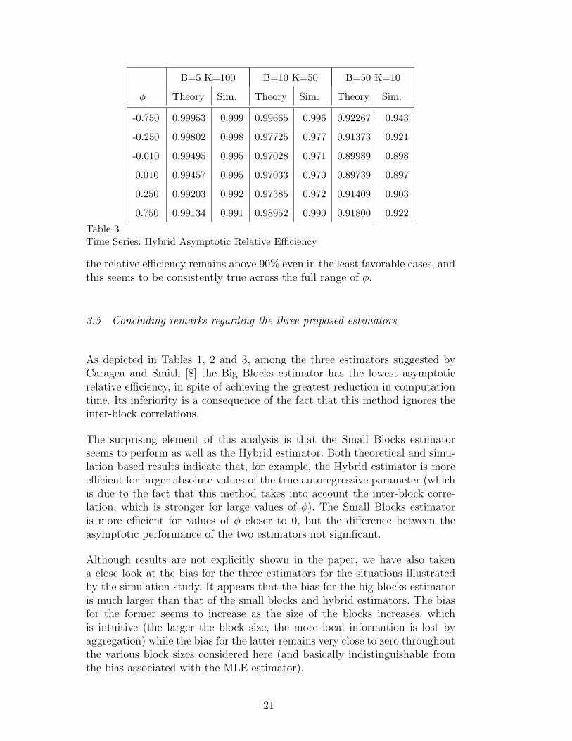
Table 3 presents the numerical results obtained for various values of φ, underthe columns labeled Theory. Calculations are performed for an AR(1) timeseries of length 500, divided into various number of blocks (5, 10 and 50), andseveral values of the autoregressive parameter φ. Under the columns labeled“Sim.”, we present results obtained through a simulation study based on 1000iterations. We note immediately that the simulated results concur with thetheoretical calculations, modulo the simulation induced error.

It is remarkable that, as illustrated by Table 3, the Hybrid estimator is veryefficient asymptotically, when compared to the maximum likelihood estimator.There is a slight decrease in efficiency when block sizes are small. Nevertheless,

20

B=5 K=100 B=10 K=50 B=50 K=10

φ Theory Sim. Theory Sim. Theory Sim.

-0.750 0.99953 0.999 0.99665 0.996 0.92267 0.943

-0.250 0.99802 0.998 0.97725 0.977 0.91373 0.921

-0.010 0.99495 0.995 0.97028 0.971 0.89989 0.898

0.010 0.99457 0.995 0.97033 0.970 0.89739 0.897

0.250 0.99203 0.992 0.97385 0.972 0.91409 0.903

0.750 0.99134 0.991 0.98952 0.990 0.91800 0.922

Table 3Time Series: Hybrid Asymptotic Relative Efficiency

the relative efficiency remains above 90% even in the least favorable cases, andthis seems to be consistently true across the full range of φ.

3.5 Concluding remarks regarding the three proposed estimators

As depicted in Tables 1, 2 and 3, among the three estimators suggested byCaragea and Smith [8] the Big Blocks estimator has the lowest asymptoticrelative efficiency, in spite of achieving the greatest reduction in computationtime. Its inferiority is a consequence of the fact that this method ignores theinter-block correlations.

The surprising element of this analysis is that the Small Blocks estimatorseems to perform as well as the Hybrid estimator. Both theoretical and simu-lation based results indicate that, for example, the Hybrid estimator is moreefficient for larger absolute values of the true autoregressive parameter (whichis due to the fact that this method takes into account the inter-block corre-lation, which is stronger for large values of φ). The Small Blocks estimatoris more efficient for values of φ closer to 0, but the difference between theasymptotic performance of the two estimators not significant.

Although results are not explicitly shown in the paper, we have also takena close look at the bias for the three estimators for the situations illustratedby the simulation study. It appears that the bias for the big blocks estimatoris much larger than that of the small blocks and hybrid estimators. The biasfor the former seems to increase as the size of the blocks increases, whichis intuitive (the larger the block size, the more local information is lost byaggregation) while the bias for the latter remains very close to zero throughoutthe various block sizes considered here (and basically indistinguishable fromthe bias associated with the MLE estimator).

21

The application of the expansion method to the one-dimensional context ofthe first order autoregressive process provides valuable insight. It confirmsthat the Big Blocks approach is not recommended on its own except for cer-tain situations, but it is one of the main components of the Hybrid method.The structure of the coefficients in the expansions of the derivatives of thepseudo-likelihood functions as quadratic sums of independent normal randomvariables allows generalization to higher dimensional setups, for which we pro-vide an illustration in the following section.

4 Application of the Expansion Method to Two-Dimensional Au-toregressive Processes on a Lattice

The purpose of this section is to illustrate how the methods of the paper canbe extended to a higher-dimensional process. Once again, the calculations thatthe method involves are highly intricate, and for this reason, we restrict ourdetailed calculations to a single simple model. Our motivation and justificationfor doing this is that by calculating asymptotic efficiencies for this example, wecan suggest some general guidelines for comparisons among the three methods,that should be applicable to more general classes of spatial processes.

4.1 General description of the two-dimensional AR(1) process and the Max-imum Likelihood Estimator

Consider a two-dimensional process Xij on a N1×N2 lattice which is assumedto be the composition of two AR(1) time series (one on each of the two di-rections defining the lattice) with the same autoregressive parameter, φ. Itfollows that the covariance structure is given by the Kronecker product of theone-dimensional covariances:

Cov[Xij, Xt`] = γ(1)it γ

(2)j` = σ2

Xφ|i−t|+|j−`|, (47)

where |φ| < 1 to ensure stationarity. Thus, we can represent the spatial processXij as

Xij − φ(Xi+1,j +Xi,j+1) + φ2Xi+1,j+1 = εij , (48)

where εij = σX(1− φ2)ξij are independent N [0, σ2ε ], σ

2ε = σ2

X(1− φ2)2. Alter-natively, we write the process in the form

Xij = σε

i∑r=−∞

j∑s=−∞

φi+j−r−sξi,j . (49)

Note that the processes we have defined here lie within the general class ofspatial processes on lattices first defined by Whittle [29].

22

The calculations leading to the maximum likelihood estimator in this case relyon the joint normal distribution of the observations {Xij, 1 ≤ i ≤ N1, 1 ≤j ≤ N2}, with mean 0 and covariance given by (47) (assume σ2

ε is known.)Using the Kronecker product notation, the covariance matrix of this processis UN1 ⊗UN2 , where UNi

for any Ni is given by (14). It follows that the inversecovariance matrix has the form U−1

N1⊗U−1

N2, with U−1

Ni(for any Ni) with entries

u∗ij as given by (16). Then the negative log likelihood function, modulo fixedconstants, is given by

N1∑i=1

N2∑j=1

N1∑t=1

N2∑`=1

XijXt`u∗iju

∗t` − log |U−1

N1⊗ U−1

N2|, (50)

4.2 Alternative Estimators

In this section we consider the spatial counterpart of the one dimensionalgrouping introduced before: assume that we divide the N1 × N2 locationson the lattice into B1 × B2 disjoint subregions, each consisting of K1 × K2

locations. That is, N1 = B1 ×K1 and N2 = B2 ×K2.

In each of the three cases examined in this section, derivations of the asymp-totic variances use the information sandwich technique. To calculate the ex-pected value of the second derivative of the pseudo log likelihood function,we exploit the properties of the underlying AR(1) covariance structure, inparticular (47), as we have for the one-dimensional setup.

To calculate the variance of the first derivative, we first expand it, using (49),as a sum of quadratic forms of independent normal random variables:∑

{r1,s1,r2,s2 : (r1,r2)<(s1,s2)}aN,r1, r2, s1, s2 ξr1r2ξs1s2 . (51)

Once the coefficients for the quadratic forms are identified, we apply Theorem2 to calculate the mean and the variance of the gradient as:

mN =∑

{r1,r2}aN,r1,r1,r2,r2 and

vN = 2∑

{r1,r2}a2

N,r1,r1,r2,r2+

∑{r1,s1,r2,s2 : (r1,r2)<(s1,s2)}

a2N,r1,r2,s1,s2

. (52)

Since the general methodology of deriving the asymptotic properties of thealternative estimators is similar to the one-dimensional case, in the subse-quent sections we give only the form of the coefficients of the quadratic forms,aN,r1,r2,s1,s2 , for each of the three situations considered in this paper, in thespatial context.

23

4.2.1 Big Blocks Estimator

This estimator is the spatial analog of the one described in Section 3.2. The BigBlocks pseudo-likelihood function is defined as the likelihood of the subregionalmeans:

pmeans(φ) =1

K21K

22

B1∑i1=1

B2∑i2=1

B1∑j1=1

B2∑j2=1

v(i1−1)B2+i2 , (j1−1)B2+j2

×K1∑

`1=1

K2∑`2=1

K1∑m1=1

K2∑m2=1

X(i1−1)K1+`1,(i2−1)K2+`2X(j1−1)K1+m1,(j2−1)K2+m2

+ log(|Vmeans|) , (53)

where Vmeans with entries vij denotes the B1B2 × B1B2 covariance matrix ofthe regional means, the derivative of its inverse is denoted by ∂φV

−1means and

has entries v′ij. Using (48) we expand the first derivative with respect to φof the function in (53) as a sum of quadratic forms of i.i.d. normal randomvariables. The coefficients of this expansion are given by:

a(1)N,r1,s1,r2,s2

= σ4ε

B1∑i1=1

B2∑i2=1

B1∑j1=1

B2∑j2=1

K1∑`1=η1

K2∑`2=η2

K1∑m1=ν1

K2∑m2=ν2

v′(i1−1)B2+i2 , (j1−1)B2+j2

×φ(i1+j1−2)K1+(i2+j2−2)K2+`1+`2+m1+m2−r1−s1−r2−s2 , (54)

and we apply Theorem 2 to obtain the variance of the first derivative of thepseudo-likelihood function. The calculation of the expected value of the secondderivative of (53) is using extensively the covariance structure of the AR(1)process.

The expression for the asymptotic variance was calculated numerically forseveral values of φ and two lattice configurations: a 32× 32 lattice with (B1 =B2 = 8,K1 = K2 = 4) and a 27×27 lattice, with (B1 = B2 = 9,K1 = K2 = 3).These results are presented in Tables 4 and 5. We note that the Big Blocksestimator is relatively inefficient compared with the MLE, but its efficiencyseems to increase while block sizes decrease. These observations are consistentwith what was noted in the one-dimensional setup.

4.2.2 Small Blocks Estimator

This subsection assumes the same setting as for the Big Blocks, with the ad-ditional assumption that the B1 × B2 blocks are independent. As in Section3.3, the relatively simpler structure of the pseudo-likelihood function enablesus to study more closely some of the theoretical aspects regarding the asymp-totic distribution of the Small Blocks estimator. If we denote by UK1K2 the

24

K1K2 × K1K2 covariance matrix corresponding to any block, whose inversehas entries u∗ij given by (16), it follows from equation (50) that the negativepseudo log likelihood function, modulo fixed constants, is given by

pSmallBlocks(φ) =B1∑

j1=1

B2∑j2=1

K1∑`1=1

K2∑`2=1

K1∑m1=1

K2∑m2=1

u∗(m1−1) K2+`1, (m2−1) K2+`2

×X(j1−1) K1+`1, (j2−1) K2+`2 X(j1−1) K1+m1, (j2−1) K2+m2

+ (B1 +B2) log |UK1K2| . (55)

Note that the function in equation (55) is a degree four polynomial in theunknown parameter φ (this is a direct consequence of the correlation structurefor the two-dimensional AR(1) process). It is straightforward to check thatthe first two conditions stated by Amemiya [2] to ensure consistency of a localmaximum are satisfied here (regarding the parameter space, measurability onthe entire parameter space and continuity in an open neighborhood of thetrue value of the parameter). Also, as stated in subsection 2.2, for the lastcondition to be satisfied, we need to have a bounded expectation of the firstorder derivative in a neighborhood of the true parameter value. This conditionis satisfied by the function in equation (55), therefore we conclude that thetwo-dimensional Small Blocks estimator is consistent.

The rest of the calculations follow the expansion technique ideas. Using (48)we expand (55) as a sum of quadratic forms of independent normal randomvariables of the form (51) . If we denote by u∗ij

′ the (i, j)-th entry of ∂φU−1K1K2

the corresponding coefficients of the expansion are given by:

aN,r1,s1,r2,s2 = σ4ε

B1∑j1=1

B2∑j2=1

K1∑`1=λ1

K2∑`2=λ2

K1∑m1=ν1

K2∑m2=ν2

u∗′(`1−1)K2+`2 , (m1−1)K2+m2

×φ2(j1−1)K1+2(j2−1)K2+`1+`2+m1+m2−r1−s1−r2−s2 . (56)

Here the lower bounds for summation are given by λ1 = f1(j1, r1, K1), λ2 =f1(j2, r2, K2), ν1 = f1(j1, s1, K1), and ν2 = f1(j2, s2, K2), where f1 and f2 aredefined by (24) and (45).

The asymptotic variance was calculated numerically for several values of φ,and two lattice configurations, as shown in Tables 4 and 5. It appears thatthe Small Blocks estimator performs very well when compared to the classi-cal maximum likelihood estimator. The loss in efficiency is remarkably low,even for configurations with small block sizes, which is the most unfavorablesituation. Given the gain in the computational time achieved when using thisestimation method, we conclude that the Small Blocks estimator is a goodalternative to the MLE for large data sets.

25

4.2.3 Hybrid Estimator

In this subsection we consider the same setting described in the previoustwo, but concentrate on the Hybrid estimator, the two-dimensional analogof the one described in detail in Section 3.4. The covariance structure underthe conditional independence assumption is much more complicated than insection 4.2.2. As a consequence, the identification of the coefficients is moreinvolved for this case, which is why we omit the technical details and onlylist them here in the form that they are used by the information sandwichtechnique. Notation is just a generalization of what we defined in the one-dimensional setting (Section 3.4):

aN,r1,s1,r2,s2 = a(1)N,r1,s1,r2,s2

+ a(2)N,r1,s1,r2,s2

+ a(3)N,r1,s1,r2,s2

+ a(4)N,r1,s1,r2,s2

,

where a(1)N,r1,s1,r2,s2

is given in expression (54) and

a(2)N,r1,s1,r2,s2

= σ4ε

B1∑j1=1

B2∑j2=1

K1∑`1=λ1

K`12∑

`2=λ∗2

K1∑m1=ν1

Km12∑

m2=ν∗2

w′(`1−1)K2+`2,(m1−1)K2+m2

× φ2(j1−1)K1+2(j2−1)K2+`1+m1+`2+m2−r1−r2−s1−s2 ,

a(3)N,r1,s1,r2,s2

= σ4ε

B1∑j1=1

B2∑j2=1

K1∑`1=λ1

K`12∑

`2=λ∗2

K1∑m1=1

Km12∑

m2=1

K1∑p1=ν1

K2∑p2=ν2

[w′

(`1−1)K2+`2,(m1−1)K2+m2τ ∗(m1−1)K2+m2

+w(`1−1)K2+`2,(m1−1)K2+m2 τ∗′(m1−1)K2+m2

]× φ2(j1−1)K1+2(j2−1)K2+`1+p1+`2+p2−r1−r2−s1−s2 ,

and

a(4)N,r1,s1,r2,s2

=σ4ε

B1∑j1=1

B2∑j2=1

K1∑`1=λ1

K`12∑

`2=λ∗2

K1∑m1=ν1

Km12∑

m2=1

K1∑p1=λ1

K2∑p2=λ2

K1∑q1=ν1

K2∑q2=ν2

[2 w(`1−1)K2+`2,(m1−1)K2+m2

× τ ∗′(`1−1)K2+`2τ ∗(m1−1)K2+m2

+ w′(`1−1)K2+`2,(m1−1)K2+m2

τ ∗(`1−1)K2+`2τ ∗(m1−1)K2+m2

]×φ2(j1−1)K1+2(j2−1)K2+p1+q1+p2+q2−r1−r2−s1−s2 .

Here the summation lower bounds are given by: η1 = f1(i1, r1, K1), η2 =f1(i2, r2, K2), λ1 = f1(j1, r1, K1), λ2 = f1(j2, r2, K2), ν1 = f1(j1, s1, K1), ν2 =f1(j2, s2, K2), λ

∗2 = f3(j2, r2, K

`22 ) and ν∗2 = f3(j2, s2, K

m22 ); functions f1 and

f2 are defined by (24) and (45), f3 is defined as:

f3(r, j, k) =

f1(r, j, k) if k = K2,

f2(r, j, k) if k = K2 − 1 ,(57)

26

while the summation upper bounds are defined as:

K`12 =

K2 if `1 < K1,

K2 − 1 if `1 = K1,and Km1

2 =

K2 if m1 < K1,

K2 − 1 if m1 = K1.(58)

The asymptotic relative efficiency was calculated numerically for various val-ues of φ and two lattice configurations. The results are presented in Tables4 and 5. We conclude that, as for the one-dimensional setup, the Hybrid es-

θ Big Blocks Small Blocks Hybrid

Efficiency Efficiency Efficiency

-0.750 0.00483 0.80386 0.80357

-0.500 0.03378 0.81132 0.81286

-0.250 0.10160 0.77615 0.78069

-0.010 0.19665 0.75005 0.75482

0.010 0.20543 0.75005 0.75468

0.250 0.31412 0.77615 0.77780

0.500 0.42135 0.81132 0.80970

0.750 0.49732 0.80386 0.80803Table 4Relative efficiency of estimators for AR(1)× AR(1) model with B1 = B2 = 8, K1 =K2 = 4.

timator is asymptotically highly efficient relative to the maximum likelihoodestimator. This, together with the significant reduction of the computationaltime, recommends it as a good estimation alternative for high dimensionaldata sets.

4.3 Conclusions

From the numerical results displayed in Tables 4 and 5 we can conclude thatthe performance of the simplest of the estimators, the Big Blocks, is inferiorto that of the other two estimators. Its asymptotic efficiency relative to theMLE increases as φ gets larger. This is caused by the dependence betweenfarther observations being stronger in this situations, which is a feature thatthe Big Blocks method is designed to capture. The other two estimators, theSmall Blocks and Hybrid are performing very well when compared to the max-imum likelihood estimator (efficiencies ranging between 68 and 80%), with noclear choice between the two. Numerical studies by Caragea and Smith [8]

27

θ Big Blocks Small Blocks Hybrid

Efficiency Efficiency Efficiency

-0.750 0.25675 0.76861 0.79230

-0.500 0.04912 0.75964 0.76768

-0.250 0.12744 0.70510 0.71818

-0.010 0.26449 0.66674 0.68148

0.010 0.27570 0.66674 0.68129

0.250 0.39986 0.70510 0.71302

0.500 0.50212 0.75964 0.75779

0.750 0.57861 0.76861 0.77155Table 5Relative efficiency of estimators for AR(1)× AR(1) model with B1 = B2 = 9, K1 =K2 = 3.

have suggested that there are some situations (spatial models where the rangeparameter is very large) in which the Big Blocks method is the best of thethree. They have also provided further numerical comparisons of the SmallBlocks and Hybrid methods that suggest that the qualitative conclusions ofthe present theoretical study hold for a much wider range of spatial models.Caragea and Smith [8] have found the Hybrid estimator to be clearly supe-rior for some settings (for example, the case of the Matern model with smallshape parameter). Another advantage of the Hybrid estimator, as illustratedby Caragea and Smith [8], is that the estimated standard errors from invertingthe approximate observed information matrix are closer to the true standarderrors than those derived by the Small Blocks method.

5 Further Discussion and Concluding remarks

This paper was intended to take a closer look at the asymptotic propertiesof the alternative estimators proposed by Caragea and Smith [8]. Since cal-culations for the general multivariate normal processes is too complicated topermit the derivation of analytical formulae for the asymptotic variances, weconsidered two particular cases: the autoregressive process of first order in oneand two dimensions. Although the covariance structure was much simpler inthese two instances than for the general spatial processes that motivated thedevelopment of the alternative estimators, derivation of closed form, easy tomanipulate formulae for the asymptotic variances was not possible. Instead,we produced and analyzed numerical results for our theoretical calculationsfor several arbitrarily chosen situations. From these considerations (Tables 1

28

through 5) we conclude that the Big Blocks estimator lacks in asymptoticefficiency, in spite of the reduction in the computational effort, in almost allcircumstances. The other two estimators perform very well asymptotically.

In the present work, we have chosen to concentrate on the statistical ratherthan computational efficiency, although the trade-off between the two could bea factor in practical applications. One may consider other conditioning choicesfor the hybrid estimator, that could lead to an even greater reduction in thecomputational effort. Such alternatives include conditioning on an arbitrarilychosen single observation or on the average of a smaller subset of observationswithin each block. It should be noted, however, that the statistical propertiesof such resulting estimators should be examined in a similar fashion to theone presented in this work.

We emphasize here that the examples illustrated by Tables 4 and 5 consideronly moderate size lattices. Even though for the specific model under consid-eration there are already several known ways of approximating the likelihoodefficiently (see Whittle [29] or Guyon [13]) or of simplifying calculations of theexact likelihood (see Zimmerman [30]), for the most general models without anexploitable structure, using the Cholesky decomposition is the most efficientmethod available to calculate the determinant and inverse of the covariancematrix. This bears the implication that using the maximum likelihood estima-tion method for a grid of 32×32 locations is on the edge of what is feasible ona single processor desktop computer. Different considerations might apply in atotally different computing environments (like parallel computing). However,these calculations could be, in principle, performed for a much larger numberof locations.

The greatest shortcoming associated with these theoretical calculations is thatthey rely heavily on the assumption that the first derivative of the pseudo-likelihood function can be expanded as a sum of quadratic forms of indepen-dent normal variables, which is not immediate for much more general spatialprocesses. However, the conclusions drawn here should remain valid for morecomplex processes, at least in the sense of recommending the Hybrid estima-tor as a reasonable competitor to the maximum likelihood estimator, for largespatial data sets.

References

[1] M. Akahira and K. Takeuchi, Asymptotic Efficiency of Statistical Estimators:Concepts and Higher Order Asymptotic Efficiency Lecture Notes in Statistics,Springer-Verlag, New York, 1981.

[2] T. Amemiya, Advanced Econometrics. Harvard University Press, Cambridge,

29

Massachusetts, 1985.

[3] S. Banerjee, B.P. Carlin, A.E. Gelfand, Hierarchichal Modeling and Analysis forSpatial Data. CRC Press/Chapman and Hall, Boca Raton, FL., 2003.

[4] R. P. Barry and R. K. Pace , Monte Carlo Estimates of the Log Determinant ofLarge Sparse Matrices, Linear Algebra and Statistics of Linear Algebra and itsApplications, 289 (1999), 41–54.

[5] P. Billingsley, Probability and Measure. Third Edition, Wiley, New York, 1995.

[6] P.J. Brockwell, R.A. Davis, Time Series: Theory and Methods. Second Edition,Springer-Verlag, New York, 1991.

[7] Billings, S. D., Beatson, R. K and Newsam, G. N., 2002, Interpolation ofgeophysical data by continuous global surfaces: Geophysics 67, 1810–1822.

[8] P.C. Caragea, R.L. Smith, Approximate Likelihoods for Spatial Processes,Submitted, 2006.

[9] J.-P. Chiles, P. Delfiner, Geostatistics: Modeling Spatial Uncertainty, John Wiley,New York, 1999.

[10] N. Cressie, Statistics for Spatial Data, John Wiley, New York, 1993.

[11] F.C. Curriero, S.R. Lele, A composite likelihood approach to semivariogramestimation, Journal of Agricultural, Biological and Environmental Statistics 4(1)(1999), 9–28.

[12] R.M. Furrer, M. Genton, D. Nychka, Covariance tapering for interpolation oflarge spatial datasets. Journal of Computational and Graphical Statistics (2006)

[13] X. Guyon, Parameter estimation for a stationary process on a d-dimensionallattice, Biometrika 69 (1982) 95–105.

[14] P.J. Heagerty, S.R. Lele, A Composite Likelihood Approach to Binary Data inSpace, Journal of thee American Statistical Association, 92 (1998) 846–854.

[15] H-C. Huang, N. Cressie, and J. Gabrosek, Fast, resolution-consistent spatialprediction of global processes from satellite data, Journal of Computational andGraphical Statistics, 11 (2002) 63–88.

[16] G. Johannesson, N. Cressie, Finding large-scale spatial trends in massive, global,environmental datasets, Environmetrics, 15 (2004) 1–44.

[17] K.Y. Liang, S.L. Zeger, Longitudinal data analysis using generalized linearmodels, Biometrika 73 (1986) 13–22.

[18] B.G. Lindsay, Composite Likelihood Methods, Contemporary Mathematics 80(1988) 221–239.

[19] D. Nychka, Spatial Process Estimates as Smoothers,Smoothing and Regression.Approaches, Computation and Application, ed. Schimek, M. G., Wiley, NewYork(2000), 393-424.

30

[20] D. Nychka, C. Wikle, J.A. Royle, Multiresolution models for nonstationaryspatial covariance functions. Statistical Modeling 2 (2002), 315–331.

[21] O. Smirnov, L. Anselin, Fast Maximum Likelihood Estimation of VeryLarge Spatial Autoregressive Models: A Characteristic Polynomial Approach,”Computational Statistics and Data Analysis 35 (3), (2001): 301–319.

[22] M.L. Stein, Interpolation of Spatial Data: Some Theory for Kriging, Springer-Verlag, New York, 1999.

[23] M.L. Stein, Z. Chi, L.J. Welty, Approximating likelihoods for large spatial datasets, J.R. Statist.Soc. B 66 (2004), 275–296.

[24] W.F. Trench, An algorithm for the inversion of finite Toeplitz matrices, J. Soc.Indust. Appl. Math. 12 (1964), 515–522.

[25] S. Tzeng, H.C. Huang, N. Cressie, A fast, optimal spatial-prediction method formassive datasets. Journal of the American Statistical Association, 100 (2005),1343–1357.

[26] A.V. Vecchia, Estimation and identification for continuous spatial processes. J.Roy. Statist B 50 (1988), 297–312.

[27] A.W. Van der Vaart, Asymptotic Statistics, Cambridge University Press, 1998.

[28] H. White, Maximum Likelihood Estimation of Misspecified Models,Econometrica 50 (1982), 1–26.

[29] P. Whittle, On stationary processes in the plane, Biometrika 41 (1954), 434–449.

[30] D.L. Zimmerman, Computationally exploitable structure of covariance matricesand generalized covariance matrices in spatial models, Journal of StatisticalComputing and Simulation 32 (1989), 1–15.

31