asynchronous and synchronous dispersals in spatially...

Copyright © by SIAM. Unauthorized reproduction of this article is prohibited.

SIAM J. APPLIED DYNAMICAL SYSTEMS c© 2008 Society for Industrial and Applied MathematicsVol. 7, No. 2, pp. 284–310

Asynchronous and Synchronous Dispersals in Spatially Discrete PopulationModels∗

Abdul-Aziz Yakubu†

Abstract. This study is on the role of synchronous and asynchronous dispersals in a discrete-time single-speciespopulation model with dispersal between two patches, where predispersal dynamics are compen-satory or overcompensatory and dispersal is synchronous or asynchronous or mixed synchronous andasynchronous. It is known that single-species dispersal-linked population models behave as single-species single-patch models whenever all predispersal local dynamics are compensatory and dispersalis synchronous. However, the dynamics of the corresponding model connected by asynchronous andmixed synchronous-asynchronous dispersals depend on the dispersal rates, intrinsic growth rates,and the parameter that models the possible modes of dispersal. The species becomes extinct onat least one patch when the asynchronous dispersal rates are high, while it persists when the ratesare low. In mixed synchronous-asynchronous systems, depending on the model parameters, thepioneer species either becomes extinct on all patches or persists on all patches. Overcompensatorypredispersal dynamics with synchronous dispersal can lead to multiple attractors with fractal basinboundaries. However, the associated models with either asynchronous or mixed synchronous andasynchronous dispersals exhibit multiple attractors with fewer numbers of distinct attractors. Thatis, the long-term dynamics of synchronous dispersal-linked systems can be more sensitive to initialpopulation sizes than that of the corresponding asynchronous and mixed synchronous-asynchronoussystems. Also, synchronous, asynchronous, and mixed synchronous-asynchronous dispersals can“stabilize” the local patch dynamics from overcompensatory to compensatory dynamics. In ourmixed synchronous-asynchronous model, the dominant mode of dispersal usually drives the dynam-ics of the full system.

Key words. asynchronous dispersal, compensatory dynamics, mixed synchronous-asynchronous dispersals, mul-tiple attractors, overcompensatory dynamics, synchronous dispersal

AMS subject classifications. 37E05, 39A11, 54H20, 92B05, 92D25, 92D40

DOI. 10.1137/070688122

1. Introduction. In host-parasite systems, the timing of density effects and parasitism canhave a profound impact on the population dynamics [35]. Doebeli made a similar observa-tion in a two-patch, single-species, dispersal-linked model of coupled Smith–Slatkin differenceequations. He showed that differences in the timing of reproduction and dispersal enhancethe stabilizing effect of dispersal [7]. Hastings [22], Gyllenberg, Soderbacka, and Ericsson [17],Doebeli [7, 8], Gonzalez-Andujar and Perry [15], and Castillo-Chavez and Yakubu [5, 44] havestudied single-species discrete-time dispersal-linked models that implicitly assume no differ-ence in the timing of reproduction and dispersal (dispersal synchrony). Their work showed that

∗Received by the editors April 12, 2007; accepted for publication (in revised form) by C. Castillo-Chavez Oc-tober 31, 2007; published electronically April 23, 2008. This research was partially supported by grants from theNational Science Foundation, the National Security Agency, and North East Fisheries Science Center (Woods Hole,MA).

http://www.siam.org/journals/siads/7-2/68812.html†Department of Mathematics, Howard University, Washington, DC 20059 ([email protected]).

284

http://www.siam.org/journals/siads/7-2/68812.html

mailto:[email protected]


ASYNCHRONOUS AND SYNCHRONOUS DISPERSAL-LINKED MODELS 285

the interaction between local dynamics and symmetric synchronous dispersal can lead to thereplacement of chaotic local dynamics by periodic dynamics for some initial population sizes.

In this paper, we introduce a single-species two-patch dispersal-linked model where predis-persal dynamics are compensatory (equilibrium dynamics) or overcompensatory (oscillatorydynamics) and dispersal is synchronous or asynchronous or mixed synchronous and asyn-chronous [2, 3, 39, 44, 45]. The novelty of our model is in the embedding of synchronousand asynchronous models into a single framework. Depending on a single continuous param-eter, the model is capable of exhibiting synchronous dispersal, asynchronous dispersal, andmixed synchronous and asynchronous dispersals. Under dispersal synchrony (that is, wherethere is no asynchronous dispersal), our model reduces to that of Hastings [22, 23], Gyllen-berg, Soderbacka, and Ericsson [17], Doebeli [7, 8], and Castillo-Chavez and Yakubu [5, 44],whereas it reduces to a model of Doebeli when dispersal is asynchronous (that is, where thereis no synchronous dispersal) [7, 8].

A large number of researchers have carried out extensive studies on the interplay betweenlocal dynamics and dispersal in dispersal-linked models. Early work on this was done byCohen and Levin [6], Gadgil [14], Hastings [23], Levin [27, 28], Levin and Paine [29], and Levins[30, 31], and later work was done by Allen [1], Doebeli [7], Doebeli and Ruxton [8], Earn, Levin,and Rohani [9], Gonzalez-Andujar and Perry [15], Gyllenberg, Soderbacka, and Ericsson [17],Hanski [18], Hanski and Gilpin [19], Hastings [22], and Castillo-Chavez and Yakubu [4, 5, 44].In this paper, we focus on the impact of synchronous and asynchronous modes of dispersalson local populations with discrete nonoverlapping generations [7, 8, 9, 15, 17, 22, 44]. Inparticular, we extend Doebeli’s idea that the detailed timing of dispersal can affect the globaldynamics of dispersal-linked systems [7, 8].

We review, in section 2, the impact of compensatory and overcompensatory dynamics on“unstructured” single-species, single-patch discrete-time models. The Beverton–Holt [2, 3, 4,5, 11, 12, 13, 20, 21, 38], bobwhite quail “hump-with-tail” [10, 44], Ricker [4, 7, 8, 22, 24,25, 32, 33, 34, 35, 36, 37, 40, 44, 45], and Smith–Slatkin [20, 36, 41, 45] models are usedto describe either compensatory or overcompensatory dynamics. Only pioneer species areconsidered (pioneer species are species that persist at very small population sizes when left inisolation with no outside interference) [11, 12, 13].

In section 3, three basic single-species dispersal-linked models consisting of two subpopu-lations (with nonoverlapping generations) connected by one of the three modes of dispersals(synchronous, asynchronous, and mixed synchronous-asynchronous dispersals) are introduced.To understand the behavior of the mixed synchronous-asynchronous model, in section 4, wereview prior work on the model with dispersal synchrony. Single-species dispersal-linked pop-ulation models under the same qualitative local compensatory dynamics are known to behaveas single-patch systems whenever dispersal is synchronous [5, 44]. When predispersal localdynamics are overcompensatory, dispersal synchrony can fracture the basins of attractionthrough its support of multiple attractors. We highlight, in section 4, the possible structuresof the coexisting attractors where local populations (in the absence of dispersal) live on eithera preselected n-cycle attractor or a chaotic attractor (overcompensatory dynamics). Hastingsand others have observed similar multiple attractors in synchronous models [4, 5, 22, 44].

The model under dispersal asynchrony is studied in sections 5 and 6. We show, in section 5,that the dynamics of the full system depend on the asynchronous dispersal rates. The species


286 ABDUL-AZIZ YAKUBU

becomes extinct on at least one patch when asynchronous dispersal rates are high, while itpersists when the rates are low. In sharp contrast to dispersal synchrony, dispersal asynchronyimpacts compensatory local dynamics [7, 23, 28, 29].

The difference in the timing of reproduction and dispersal enlarges the asynchrony of inter-actions, and Doebeli predicted the “likelihood” of simple system dynamics due to asynchronousdispersal [7]. In general, dispersal can give rise to multiple attractors with interesting basinstructures, whenever the local patch dynamics are overcompensatory [4, 5, 7, 9, 16, 19, 22, 26,44]. In section 6, several examples are introduced to show that dispersal-linked models with“unstructured” overcompensatory predispersal patch dynamics connected by asynchronoussymmetric or asymmetric dispersal support multiple attractors with a smaller number of dis-tinct attractors than the corresponding model under dispersal synchrony. We use MATLABand the Dynamics software of Nusse and Yorke to study the differences among the structures ofthe attractors and the differences between the synchronous and asynchronous cases [39]. Ourresults show that asynchronous dispersal can stabilize or shift the predispersal local dynamicsfrom an attracting period four to a period two or to a fixed point or to a limit cycle attractor.That is, both synchronous and asynchronous dispersals can generate period-doubling reversalsin dispersal-linked models under overcompensatory dynamics.

Models under mixed synchronous-asynchronous dispersals are studied in sections 7, 8,and 9. As in synchronous models, in mixed models, the pioneer species either persists on allpatches or becomes extinct on all patches. In section 7, we derive conditions for the extinction(respectively, persistence) of the species on all patches. Mixed synchronous-asynchronoussystems under compensatory and overcompensatory local dynamics are studied in sections 8and 9, respectively. When the local dynamics are overcompensatory, mixed models exhibitmultiple attractors with a smaller number of distinct attractors than the corresponding modelunder dispersal asynchrony. Section 10 discusses some possible implications of the resultsof this paper, and relevant mathematical details of all technical terms are collected in theappendix.

2. Predispersal local patch dynamics. In this section, we review single-species discrete-time population models without dispersal. As in [7, 22, 44], the equation for the local dynamicsin each Patch i ∈ {1, 2} at generation t after reproduction but before dispersal is modeled by

(1) xi(t + 1) = xi(t)gi(xi(t)) (i = 1, 2),

where xi(t) denotes the population size and the per capita growth functions, gi : [0,∞) →(0,∞) are assumed to be strictly decreasing, positive, and twice differentiable (C2 on [0,∞)),where gi(0) > 1 and limxi→∞ gi(xi) < 1. System (1) is a discrete-time, single-species, popu-lation model with two (uncoupled) patches. It describes the population dynamics of pioneerspecies [4, 5, 11, 12, 13, 44].

Predispersal Patch i local reproduction function fi(xi) = xigi(xi) describes the local dy-namics of the species, where xi is the measure of the size of the population in the patch. Eachfi has a unique positive fixed point denoted by Xi. Since gi is a strictly decreasing continuousfunction, fi(xi) > xi whenever 0 < xi < Xi and fi(xi) < xi whenever xi > Xi. Consequently,Ii ≡ fi([0, Xi]) is a global attractor. That is, every initial population eventually reaches alimit in Ii.



We focus on two types of local dynamics—compensatory and overcompensatory dynamics.Definition 1. Patch i predispersal local dynamics are compensatory whenever all positive

population sizes approach the positive equilibrium at Xi monotonically under fi iterations[4, 38, 44].

Definition 2. Patch i predispersal local dynamics are overcompensatory whenever some pos-itive population sizes “overshoot” the positive equilibrium at Xi under fi iterations (that is,f

′i (Xi) < 0) [4, 38, 44].

If fi increases monotonically from zero with the rate of increase slowing down as xi getslarge, then all population sizes “undershoot” the globally attracting positive equilibrium, andby Definition 1 Patch i local dynamics are compensatory. The Beverton–Holt stock recruit-ment model, fi(xi) = aixi

1+bixi, portrays compensatory dynamics in Patch i whenever ai > 1

and bi > 0 [4, 44, 45]. If fi is an orientation-reversing one-hump map with a stable positivefixed point (respectively, an unstable positive fixed point), then the return to the stable fixedpoint takes the form of damped oscillations (respectively, the local behavior near the unstablefixed point takes the form of divergent oscillations), and by Definition 2 Patch i dynamicsare overcompensatory. Whenever ri > 1 and fi is Ricker’s model, fi(xi) = xi exp(ri − xi),then the dynamics in Patch i are overcompensatory [2, 3, 4, 5, 7, 8, 9, 10, 11, 12, 13, 20,21, 22, 32, 33, 34, 35, 36, 37, 38, 39, 40, 44, 45]. In general, fi supports either an n-cycle(nonchaotic) attractor with n > 1 or a chaotic (interval) attractor whenever Patch i dynamicsare overcompensatory and the positive fixed point is unstable.

A detailed description of functions under compensatory or overcompensatory dynamicsrequires the introduction of the concept of an α-monotone concave map.

Definition 3. fi is an α-monotone concave map if f′i (xi) > 0 and f

′′i (xi) < 0 for each

xi ∈ [0, α) [4, 38, 44].Patch i population is under compensatory dynamics at population sizes in the interval

[0, α) whenever fi is an α-monotone concave map with a unique positive fixed point in theopen interval (0, α) (see [44, Definition 3]). The bobwhite quail “hump-with-tail” modelfi(xi) = xi(ki + Ki

1+xini ), the Ricker model fi(xi) = xi exp(ri − xi), and the Smith–Slatkin

model fi(xi) = aixi

1+(bixi)lidescribe overcompensatory and compensatory dynamics (depending

on parameter values). If li = 1 and ai > 1, the Smith–Slatkin model reduces to the Beverton–Holt model, an ∞-monotone concave map (compensatory dynamics [2, 36, 42, 44]).

3. Synchronous and asynchronous dispersal-linked two-patch model. Hastings [22],Gyllenberg, Soderbacka, and Ericsson [17], Doebeli [7, 8], Yakubu and Castillo-Chavez [44],and others have studied discrete-time single-species dispersal-linked population models thatimplicitly assume that the timing of reproduction and dispersal do not differ from patch topatch. A two-patch version of these models with dispersal synchrony is given by the followingsystem of coupled nonlinear difference equations:

(2)x1(t + 1) = (1 − d1)f1(x1(t)) + d2f2(x2(t)),x2(t + 1) = d1f1(x1(t)) + (1 − d2)f2(x2(t)).

}

In system (2), reproduction occurs prior to dispersal within each generation and in each patch.After reproduction, the constant fraction d1 ∈ (0, 1) of the population disperses from Patch 1to Patch 2 while the constant fraction d2 ∈ (0, 1) disperses from Patch 2 to Patch 1.



Doebeli, in 1995, studied a simple two-patch discrete-time model of coupled Smith–Slatkinsingle-species ecological models where the timing of reproduction and dispersal differs frompatch to patch. In Doebeli’s two-patch model, in each generation reproduction occurs inPatch 1 first, followed by the dispersal, from Patch 1 to Patch 2, of the fraction d1 of thepopulation. As a result, Patch 2 population experiences the effects of its own density as wellas that of the newly dispersed individuals from Patch 1 to Patch 2. In Patch 2, the fractiond2 of the population disperses from Patch 2 to Patch 1 after reproduction [7]. The dynamicsof the two-patch system under asynchronous dispersal are then described by the followingsystem of coupled nonlinear difference equations:

(3)x1(t + 1) = (1 − d1)f1(x1(t)) + d2x2(t)g2(x2(t) + d1f1(x1(t))),x2(t + 1) = (1 − d2)x2(t)g2(x2(t) + d1f1(x1(t))),

}

where 0 < d1, d2 < 1 and f1(x1) = x1g1(x1).

In Doebeli’s simple model with dispersal asynchrony, at the next generation, the popula-tion size in Patch 1 is increased by the dispersal from Patch 2. However, unlike the Patch 1population size, the population size in Patch 2 at the next generation is not increased by thedispersal from Patch 1. By their own nature, such simple models do not incorporate manyof the important biological factors. However, they often provide useful insights to help ourunderstanding of complex processes.

To embed synchronous and asynchronous dispersals into a single framework, we let theconstant parameter γ ∈ [0, 1] span the range of possible modes of dispersal, where γ = 0 impliessynchronous dispersal, γ = 1 implies asynchronous dispersal, and γ ∈ (0, 1) implies mixedsynchronous and asynchronous dispersal. This leads to the following equations describing thedispersal phase:

(4)x1(t + 1) = F1(x1(t), x2(t)) = (1 − d1)f1(x1(t)) + d2x2(t)g2(x(t)),x2(t + 1) = F2(x1(t), x2(t)) = (1 − γ)d1f1(x1(t)) + (1 − d2)x2(t)g2(x(t)),

}

where

x(t) = x2(t) + γd1f1(x1(t)).

Unlike Doebeli’s model, in models (2) and (4), at the next generation the population sizein Patch 1 is increased by the dispersal from Patch 2, while that of Patch 2 is increased by thedispersal from Patch 1. In each generation, reproductions in Patch 2 of models (3) and (4)experience crowding from the dispersal from Patch 1.

The vector of population densities x(t) = (x1(t), x2(t)) is written as x = (x1, x2) so thatthe dispersal-linked function is

F : R2+ → R

2+,

where

F (x1, x2) = (F1(x1, x2), F2(x1, x2)).

Then F t is the dispersal-linked function composed with itself t times. F ti (x) is the ith com-

ponent of F t evaluated at the point x in R2+. In system (4), F t gives the population densities

in generation t.



When γ = 0 (respectively, γ = 1), dispersal is synchronous (respectively, asynchronous),and system (4) reduces to system (2) (respectively, system (3)). Dispersal is symmetric whend1 = d2, while it is asymmetric when d1 �= d2. When there are no dispersals, d1 = d2 = 0and system (4) reduces to the uncoupled system (1). The predispersal basic demographicreproductive number in each patch (d1 = d2 = 0) is

�id = gi(0).

�id > 1 guarantees the successful invasion and survival of the discretely reproducing population

in Patch i, while �id < 1 guarantees the extinction of the initial population in the patch (no

dispersal). We assume throughout that the species is a pioneer in each Patch i ∈ {1, 2}. Thatis, �i

d > 1.In system (4), there is no population explosion.Lemma 1. In system (4), the positive cone is positively invariant and no point has an

unbounded orbit.

4. Dispersal synchrony in two-patch models. In this section, we consider system (4) withonly dispersal synchrony (that is, system (2) or system (4) with γ = 0). Others have studiedsynchronous dispersal models, and in this section we review some of these prior works. Whenall local dynamics are compensatory, Yakubu and Castillo-Chavez proved that system (2)supports a positive equilibrium that attracts all positive initial population sizes [44]. Thatis, when all local dynamics are compensatory, the qualitative dynamics of system (2) withsymmetric or asymmetric synchronous dispersal between patches is qualitatively equivalentto those of each of the local single patches before dispersal. With synchronous symmetricdispersal and symmetric initial population sizes, system (2) behaves as a single patch systemwhenever the local reproduction functions are identical (f1 = f2) and the predispersal localdynamics are either compensatory or overcompensatory.

In 1993, Hastings [22] and Gyllenberg, Soderbacka, and Ericsson [17] used two identical lo-gistic difference equations in system (2) with parameters in the chaotic regime to illustrate thatsynchronous dispersal-linked population models are capable of supporting multiple attractorswith complicated attraction-basin boundaries. In a recent paper, Yakubu and Castillo-Chavezstudied the role of synchronous dispersal in generating multiple attractors where local dynam-ics are overcompensatory [44]. They focused on situations where the local populations (in theabsence of dispersal) live on either a preselected n-cycle attractor or a chaotic attractor.Yakubu and Castillo-Chavez supported the results of Hastings and obtained that synchronousdispersal can force the preselected (chaotic or nonchaotic) attractor to coexist with one ormore “new” attractors (multiple attractors). Example 1 illustrates multiple attractors in sys-tem (2) with synchronous symmetric dispersal, where the local dynamics are governed by theRicker model. In Example 1, we choose the values of the parameters so that the predispersallocal dynamics and the full system dynamics under synchronous symmetric dispersal are aslisted in Table 1.

Example 1. Consider system (2) with the Ricker model

fi(xi) = xi exp(ri − xi)

for each i ∈ {1, 2}. Set the following parameter values:

r = r1 = r2 ∈ (2, 2.52) and d1 = d2 = 0.03.



Table 1Predispersal local dynamics versus postdispersal synchronous dynamics.

r values Predispersal attractors Synchronous attractors

1. (2, 2.53) 2-cycle two 2-cycles (see Fig. 1)

2. (2.53, 2.59) 4-cycle 4- and 2-cycles

3. (2.66, 2.68) 8-cycle 8-, 4-, and 2-cycles

4. (2.69, 2.6901) 16-cycle 16-, 8-, 4-, and 2-cycles

5. (2.695, 2.701) chaotic attractor four attractors (see Fig. 2)

Figure 1. Two coexisting attractors: Symmetric 2-cycle (red dots) and an asymmetric 2-cycle (blue dots)in the (x1, x2)-plane, where r1 = r2 = 2.1 and d1 = d2 = 0.03. Figure 1 is plotted over 3000 time steps.

Figure 2. Four attractors: Symmetric 4-piece chaotic attractor (blue region), asymmetric 4-cycle (greendots), asymmetric 16-cycle (red dots), and a period-2 limit cycle (black region), where r1 = r2 = 2.7 andd1 = d2 = 0.03. Figure 2 is plotted over 5000 time steps.

The predispersal local dynamics in Example 1, fi(xi) = xi exp(ri − xi), have a stable pos-itive fixed point at Xi = ri whenever 0 < ri < 2 [44]. As ri is increased past 2, the fixed pointXi undergoes a period-doubling bifurcation route to chaos [33, 34, 35, 39]. In Example 1,the predispersal identical local patches are on a 2-cycle attractor (overcompensatory dynam-ics), and the full system with symmetric dispersal supports multiple attractors—a symmetric2-cycle attractor coexisting with an asymmetric 2-cycle attractor (see Figure 1 and Table 1).To study the impact of increasing the identical intrinsic growth rates, r = r1 = r2, thesymmetric dispersal rates are kept fixed at d1 = d2 = 0.03 while r is increased past 2.52.



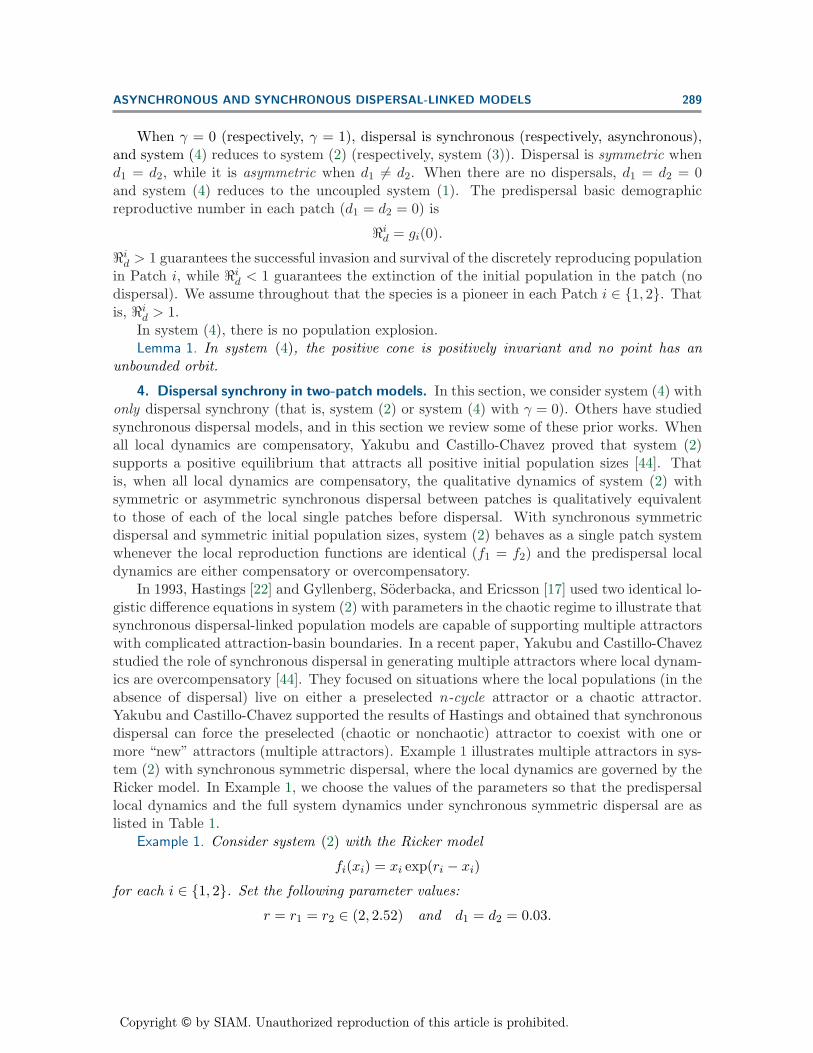
Figure 3. Basins of attraction of two coexisting 2-cycle attractors, where the parameters are exactly as inFigure 1. The white region is the basin of attraction of the black “specks” ( 2-cycle) in the figure, and the blackregion is the basin of attraction of the other coexisting attractor. On the horizontal axis 0 ≤ x1 ≤ 4, and onthe vertical axis 0 ≤ x2 ≤ 4. Figure 3 is plotted over 5000 time steps.

When r ∈ (2.53, 2.59), the predispersal identical local patches are on a 4-cycle attrac-tor, and the full system with symmetric dispersal supports two coexisting attractors con-sisting of a symmetric 4-cycle attractor and an asymmetric 2-cycle attractor (see Table 1).At r ∈ (2.6, 2.65), the predispersal identical local patches are on a 4-cycle attractor, whilethe full system with symmetric dispersal supports three coexisting attractors consisting ofa symmetric 4-cycle attractor, an asymmetric 4-cycle attractor, and an asymmetric 2-cycleattractor (see Table 1). For values of r ∈ (2.66, 2.68), the predispersal identical local patchesare on an 8-cycle attractor, and the full system with symmetric dispersal supports three coex-isting attractors consisting of a symmetric 8-cycle attractor, an asymmetric 4-cycle attractor,and an asymmetric 2-cycle attractor (see Table 1). At r ∈ (2.69, 2.6901), the predispersalidentical local patches are on a 16-cycle attractor, while the full system with symmetric dis-persal supports four coexisting attractors consisting of a symmetric 16-cycle attractor, anasymmetric 8-cycle attractor, an asymmetric 4-cycle attractor, and an asymmetric 2-cycleattractor (see Table 1). When r ∈ (2.695, 2.701), the predispersal identical local patches areon a chaotic attractor, and the full system with symmetric dispersal supports four coexist-ing attractors consisting of a symmetric chaotic attractor, a period-2 limit cycle attractor,an asymmetric 4-cycle attractor, and an asymmetric 16-cycle attractor (see Figure 2 andTable 1).

The qualitative structure and number of the attractors in dispersal-linked populationmodels are the result of a complex interaction between the dispersal rate and predispersallocal patch dynamics. The basins of attraction, the set of all population sizes that eventuallysettle into an attractor under iteration, may provide critical information on a variety of issuesincluding the final attractor observed. In Example 1, the Dynamics software of Nusse andYorke is used to study the nature of the basins of attraction of the multiple attractors inFigures 1 and 2 [39]. As in [44], Figures 3 and 4 highlight that the basins of attraction



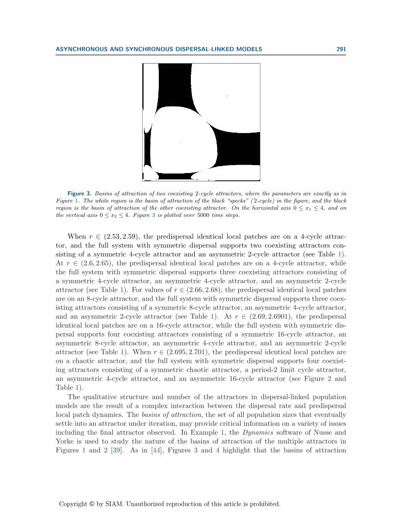
Figure 4. Basins of attraction of the 4 attractors, where the parameters are exactly as in Figure 2. On thehorizontal axis 0 ≤ x1 ≤ 6, and on the vertical axis 0 ≤ x2 ≤ 6. Figure 4 is plotted over 5000 time steps.

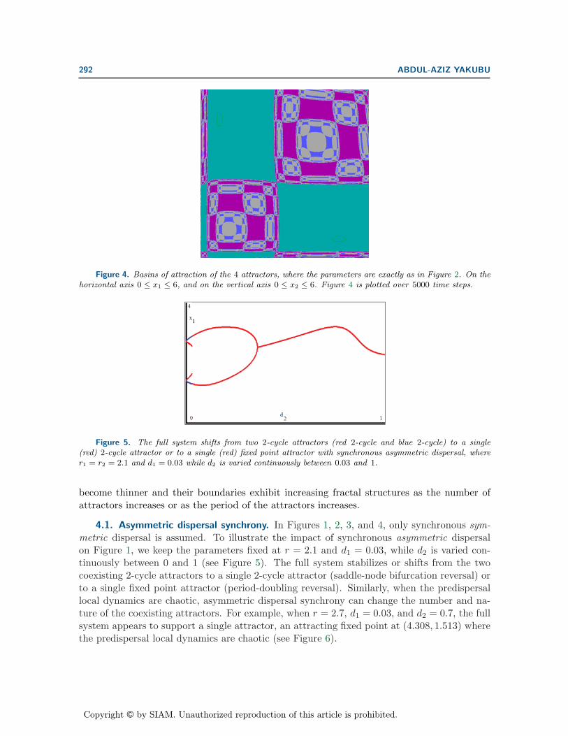
Figure 5. The full system shifts from two 2-cycle attractors (red 2-cycle and blue 2-cycle) to a single(red) 2-cycle attractor or to a single (red) fixed point attractor with synchronous asymmetric dispersal, wherer1 = r2 = 2.1 and d1 = 0.03 while d2 is varied continuously between 0.03 and 1.

become thinner and their boundaries exhibit increasing fractal structures as the number ofattractors increases or as the period of the attractors increases.

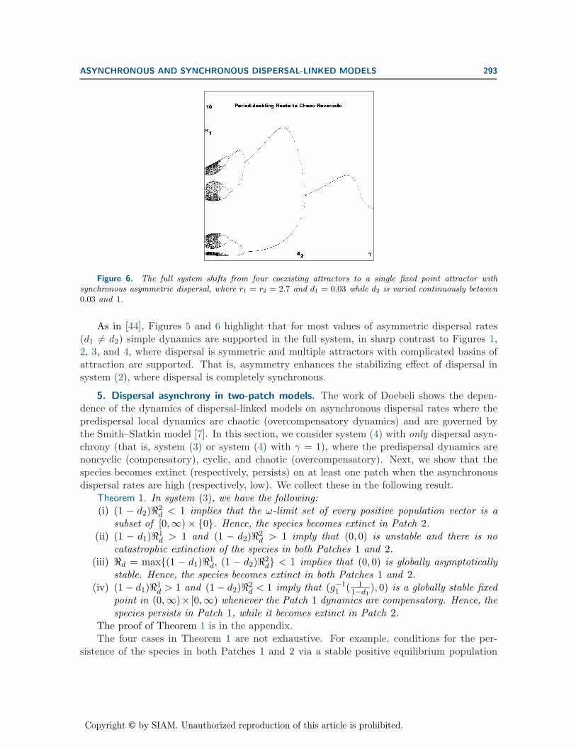
4.1. Asymmetric dispersal synchrony. In Figures 1, 2, 3, and 4, only synchronous sym-metric dispersal is assumed. To illustrate the impact of synchronous asymmetric dispersalon Figure 1, we keep the parameters fixed at r = 2.1 and d1 = 0.03, while d2 is varied con-tinuously between 0 and 1 (see Figure 5). The full system stabilizes or shifts from the twocoexisting 2-cycle attractors to a single 2-cycle attractor (saddle-node bifurcation reversal) orto a single fixed point attractor (period-doubling reversal). Similarly, when the predispersallocal dynamics are chaotic, asymmetric dispersal synchrony can change the number and na-ture of the coexisting attractors. For example, when r = 2.7, d1 = 0.03, and d2 = 0.7, the fullsystem appears to support a single attractor, an attracting fixed point at (4.308, 1.513) wherethe predispersal local dynamics are chaotic (see Figure 6).



Figure 6. The full system shifts from four coexisting attractors to a single fixed point attractor withsynchronous asymmetric dispersal, where r1 = r2 = 2.7 and d1 = 0.03 while d2 is varied continuously between0.03 and 1.

As in [44], Figures 5 and 6 highlight that for most values of asymmetric dispersal rates(d1 �= d2) simple dynamics are supported in the full system, in sharp contrast to Figures 1,2, 3, and 4, where dispersal is symmetric and multiple attractors with complicated basins ofattraction are supported. That is, asymmetry enhances the stabilizing effect of dispersal insystem (2), where dispersal is completely synchronous.

5. Dispersal asynchrony in two-patch models. The work of Doebeli shows the depen-dence of the dynamics of dispersal-linked models on asynchronous dispersal rates where thepredispersal local dynamics are chaotic (overcompensatory dynamics) and are governed bythe Smith–Slatkin model [7]. In this section, we consider system (4) with only dispersal asyn-chrony (that is, system (3) or system (4) with γ = 1), where the predispersal dynamics arenoncyclic (compensatory), cyclic, and chaotic (overcompensatory). Next, we show that thespecies becomes extinct (respectively, persists) on at least one patch when the asynchronousdispersal rates are high (respectively, low). We collect these in the following result.

Theorem 1. In system (3), we have the following:(i) (1 − d2)�2

d < 1 implies that the ω-limit set of every positive population vector is asubset of [0,∞) × {0}. Hence, the species becomes extinct in Patch 2.

(ii) (1 − d1)�1d > 1 and (1 − d2)�2

d > 1 imply that (0, 0) is unstable and there is nocatastrophic extinction of the species in both Patches 1 and 2.

(iii) �d = max{(1 − d1)�1d, (1 − d2)�2

d} < 1 implies that (0, 0) is globally asymptoticallystable. Hence, the species becomes extinct in both Patches 1 and 2.

(iv) (1 − d1)�1d > 1 and (1 − d2)�2

d < 1 imply that (g−11 ( 1

1−d1), 0) is a globally stable fixed

point in (0,∞)× [0,∞) whenever the Patch 1 dynamics are compensatory. Hence, thespecies persists in Patch 1, while it becomes extinct in Patch 2.

The proof of Theorem 1 is in the appendix.The four cases in Theorem 1 are not exhaustive. For example, conditions for the per-

sistence of the species in both Patches 1 and 2 via a stable positive equilibrium population



vector can be obtained if one assumes the persistence of the species in Patch 2 where the asyn-chronous dispersal rates are low and the local dynamics are compensatory. To illustrate thisin the simplest setting, we assume that the predispersal Patch 1 local population has reachedthe positive equilibrium X1, and we let f1(x1) ≡ X1 [43, 46]. Then system (3) reduces to thesystem

(5)x1(t + 1) = (1 − d1)X1 + d2x2(t)g2(x2(t) + d1X1),x2(t + 1) = (1 − d2)x2(t)g2(x2(t) + d1X1).

}

If the dispersal rate from Patch 2 to Patch 1 is low, then system (5) supports a globallystable positive equilibrium whenever the predispersal local patch dynamics are compensatoryand the Patch 1 carrying capacity is small. That is, dispersal asynchrony like dispersal syn-chrony is capable of supporting the persistence of the pioneer species in all patches. Wesummarize these in the following result.

Theorem 2. In system (5), let each local patch dynamics be modeled by fi, an α-monotoneconcave map, with the positive fixed point Xi ∈ (0, α). If (1 − d2)�2

d > 1, then the positiveequilibrium population vector,(

(1 − d1)X1 +d2

1 − d2

(g−12

(1

1 − d2

)− d1X1

), g−1

2

(1

1 − d2

)− d1X1

),

is globally attracting whenever X1 <g−12 ( 1

1−d2)

d1. That is, the dispersal-linked system supports

a globally stable positive fixed point whenever the predispersal local patch dynamics are com-pensatory.

The proof of Theorem 2 is in the appendix.

In Example 2, we use compensatory local dynamics via the Beverton–Holt model to illus-trate the dependence of the dynamics of system (3) on the asynchronous dispersal rates.

Example 2. Consider system (3) with

fi(xi) =aixi

1 + bixi


a1 = 2, a2 = 2.1, b1 = b2 = 1, and d1 = d2 = 0.01.

In Example 2, the local dynamics in both patches are compensatory, where g1(0) = a1,

g2(0) = a2, X1 = 0.01, X2 = 0.1, (1 − d2)�2d > 1, and X1 <

g−12 ( 1

1−d2)

d1. Consequently, the

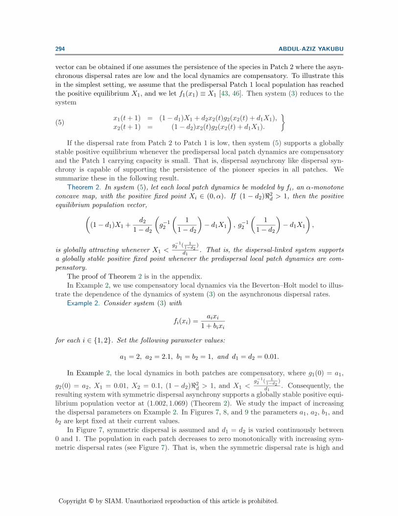
resulting system with symmetric dispersal asynchrony supports a globally stable positive equi-librium population vector at (1.002, 1.069) (Theorem 2). We study the impact of increasingthe dispersal parameters on Example 2. In Figures 7, 8, and 9 the parameters a1, a2, b1, andb2 are kept fixed at their current values.

In Figure 7, symmetric dispersal is assumed and d1 = d2 is varied continuously between0 and 1. The population in each patch decreases to zero monotonically with increasing sym-metric dispersal rates (see Figure 7). That is, when the symmetric dispersal rate is high and



Figure 7. When the symmetric dispersal rate d1 = d2 is low the species persists in both Patches 1 and 2.However, when d1 = d2 > 0.53 it becomes extinct in both Patches 1 and 2.

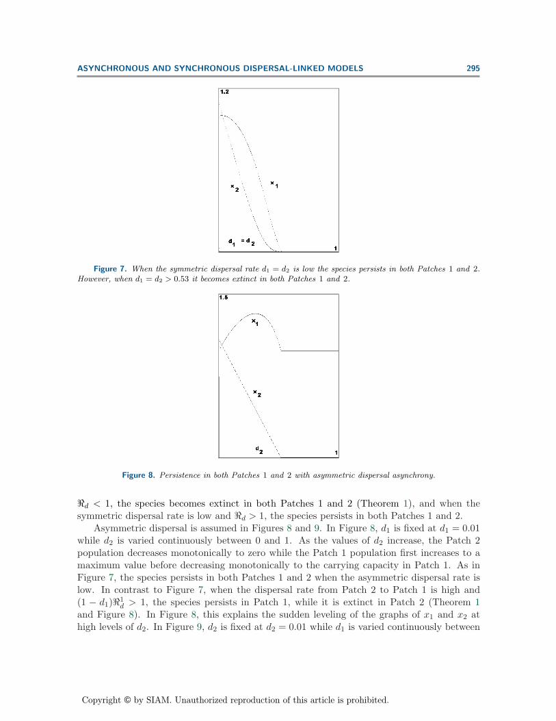
Figure 8. Persistence in both Patches 1 and 2 with asymmetric dispersal asynchrony.

�d < 1, the species becomes extinct in both Patches 1 and 2 (Theorem 1), and when thesymmetric dispersal rate is low and �d > 1, the species persists in both Patches 1 and 2.

Asymmetric dispersal is assumed in Figures 8 and 9. In Figure 8, d1 is fixed at d1 = 0.01while d2 is varied continuously between 0 and 1. As the values of d2 increase, the Patch 2population decreases monotonically to zero while the Patch 1 population first increases to amaximum value before decreasing monotonically to the carrying capacity in Patch 1. As inFigure 7, the species persists in both Patches 1 and 2 when the asymmetric dispersal rate islow. In contrast to Figure 7, when the dispersal rate from Patch 2 to Patch 1 is high and(1 − d1)�1

d > 1, the species persists in Patch 1, while it is extinct in Patch 2 (Theorem 1and Figure 8). In Figure 8, this explains the sudden leveling of the graphs of x1 and x2 athigh levels of d2. In Figure 9, d2 is fixed at d2 = 0.01 while d1 is varied continuously between



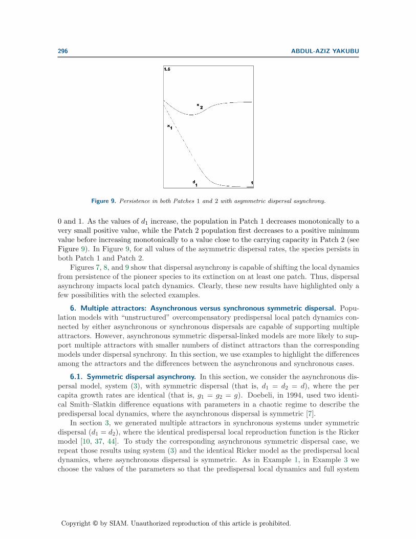
Figure 9. Persistence in both Patches 1 and 2 with asymmetric dispersal asynchrony.

0 and 1. As the values of d1 increase, the population in Patch 1 decreases monotonically to avery small positive value, while the Patch 2 population first decreases to a positive minimumvalue before increasing monotonically to a value close to the carrying capacity in Patch 2 (seeFigure 9). In Figure 9, for all values of the asymmetric dispersal rates, the species persists inboth Patch 1 and Patch 2.

Figures 7, 8, and 9 show that dispersal asynchrony is capable of shifting the local dynamicsfrom persistence of the pioneer species to its extinction on at least one patch. Thus, dispersalasynchrony impacts local patch dynamics. Clearly, these new results have highlighted only afew possibilities with the selected examples.

6. Multiple attractors: Asynchronous versus synchronous symmetric dispersal. Popu-lation models with “unstructured” overcompensatory predispersal local patch dynamics con-nected by either asynchronous or synchronous dispersals are capable of supporting multipleattractors. However, asynchronous symmetric dispersal-linked models are more likely to sup-port multiple attractors with smaller numbers of distinct attractors than the correspondingmodels under dispersal synchrony. In this section, we use examples to highlight the differencesamong the attractors and the differences between the asynchronous and synchronous cases.

6.1. Symmetric dispersal asynchrony. In this section, we consider the asynchronous dis-persal model, system (3), with symmetric dispersal (that is, d1 = d2 = d), where the percapita growth rates are identical (that is, g1 = g2 = g). Doebeli, in 1994, used two identi-cal Smith–Slatkin difference equations with parameters in a chaotic regime to describe thepredispersal local dynamics, where the asynchronous dispersal is symmetric [7].

In section 3, we generated multiple attractors in synchronous systems under symmetricdispersal (d1 = d2), where the identical predispersal local reproduction function is the Rickermodel [10, 37, 44]. To study the corresponding asynchronous symmetric dispersal case, werepeat those results using system (3) and the identical Ricker model as the predispersal localdynamics, where asynchronous dispersal is symmetric. As in Example 1, in Example 3 wechoose the values of the parameters so that the predispersal local dynamics and full system



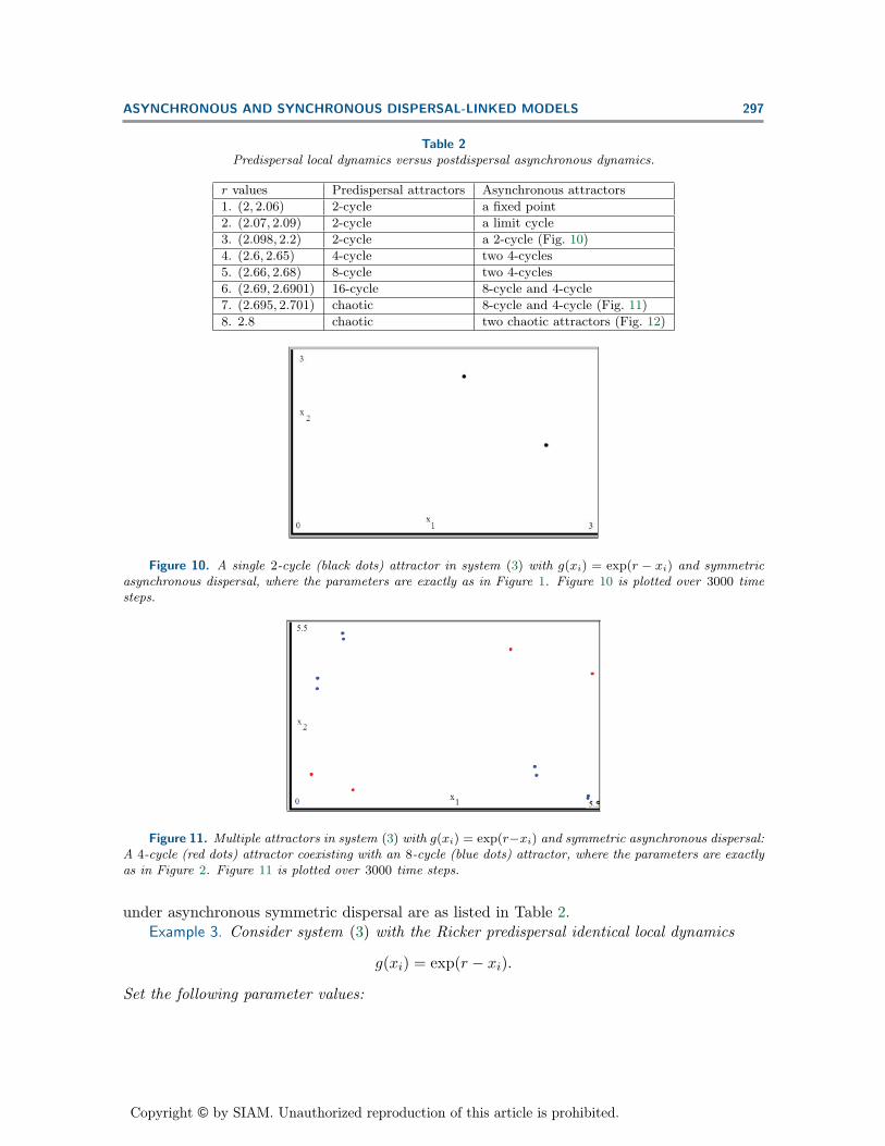
Table 2Predispersal local dynamics versus postdispersal asynchronous dynamics.

r values Predispersal attractors Asynchronous attractors

1. (2, 2.06) 2-cycle a fixed point

2. (2.07, 2.09) 2-cycle a limit cycle

3. (2.098, 2.2) 2-cycle a 2-cycle (Fig. 10)

4. (2.6, 2.65) 4-cycle two 4-cycles

5. (2.66, 2.68) 8-cycle two 4-cycles

6. (2.69, 2.6901) 16-cycle 8-cycle and 4-cycle

7. (2.695, 2.701) chaotic 8-cycle and 4-cycle (Fig. 11)

8. 2.8 chaotic two chaotic attractors (Fig. 12)

Figure 10. A single 2-cycle (black dots) attractor in system (3) with g(xi) = exp(r − xi) and symmetricasynchronous dispersal, where the parameters are exactly as in Figure 1. Figure 10 is plotted over 3000 timesteps.

Figure 11. Multiple attractors in system (3) with g(xi) = exp(r−xi) and symmetric asynchronous dispersal:A 4-cycle (red dots) attractor coexisting with an 8-cycle (blue dots) attractor, where the parameters are exactlyas in Figure 2. Figure 11 is plotted over 3000 time steps.

under asynchronous symmetric dispersal are as listed in Table 2.Example 3. Consider system (3) with the Ricker predispersal identical local dynamics

g(xi) = exp(r − xi).

Set the following parameter values:



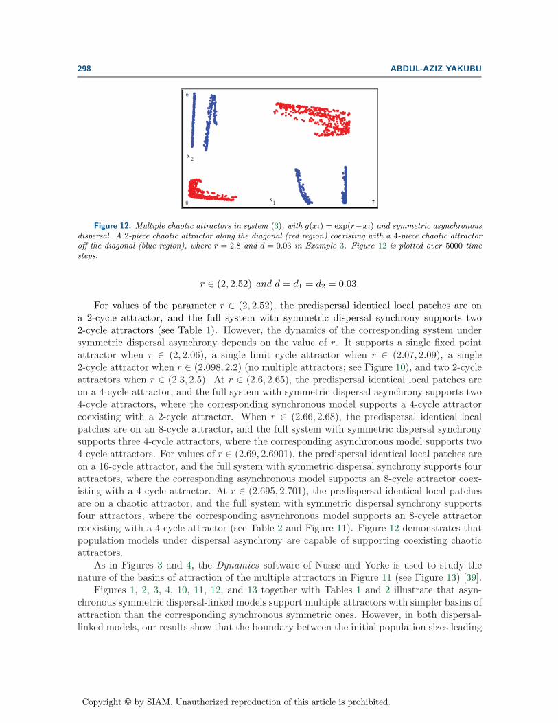
Figure 12. Multiple chaotic attractors in system (3), with g(xi) = exp(r−xi) and symmetric asynchronousdispersal. A 2-piece chaotic attractor along the diagonal (red region) coexisting with a 4-piece chaotic attractoroff the diagonal (blue region), where r = 2.8 and d = 0.03 in Example 3. Figure 12 is plotted over 5000 timesteps.

r ∈ (2, 2.52) and d = d1 = d2 = 0.03.

For values of the parameter r ∈ (2, 2.52), the predispersal identical local patches are ona 2-cycle attractor, and the full system with symmetric dispersal synchrony supports two2-cycle attractors (see Table 1). However, the dynamics of the corresponding system undersymmetric dispersal asynchrony depends on the value of r. It supports a single fixed pointattractor when r ∈ (2, 2.06), a single limit cycle attractor when r ∈ (2.07, 2.09), a single2-cycle attractor when r ∈ (2.098, 2.2) (no multiple attractors; see Figure 10), and two 2-cycleattractors when r ∈ (2.3, 2.5). At r ∈ (2.6, 2.65), the predispersal identical local patches areon a 4-cycle attractor, and the full system with symmetric dispersal asynchrony supports two4-cycle attractors, where the corresponding synchronous model supports a 4-cycle attractorcoexisting with a 2-cycle attractor. When r ∈ (2.66, 2.68), the predispersal identical localpatches are on an 8-cycle attractor, and the full system with symmetric dispersal synchronysupports three 4-cycle attractors, where the corresponding asynchronous model supports two4-cycle attractors. For values of r ∈ (2.69, 2.6901), the predispersal identical local patches areon a 16-cycle attractor, and the full system with symmetric dispersal synchrony supports fourattractors, where the corresponding asynchronous model supports an 8-cycle attractor coex-isting with a 4-cycle attractor. At r ∈ (2.695, 2.701), the predispersal identical local patchesare on a chaotic attractor, and the full system with symmetric dispersal synchrony supportsfour attractors, where the corresponding asynchronous model supports an 8-cycle attractorcoexisting with a 4-cycle attractor (see Table 2 and Figure 11). Figure 12 demonstrates thatpopulation models under dispersal asynchrony are capable of supporting coexisting chaoticattractors.

As in Figures 3 and 4, the Dynamics software of Nusse and Yorke is used to study thenature of the basins of attraction of the multiple attractors in Figure 11 (see Figure 13) [39].

Figures 1, 2, 3, 4, 10, 11, 12, and 13 together with Tables 1 and 2 illustrate that asyn-chronous symmetric dispersal-linked models support multiple attractors with simpler basins ofattraction than the corresponding synchronous symmetric ones. However, in both dispersal-linked models, our results show that the boundary between the initial population sizes leading



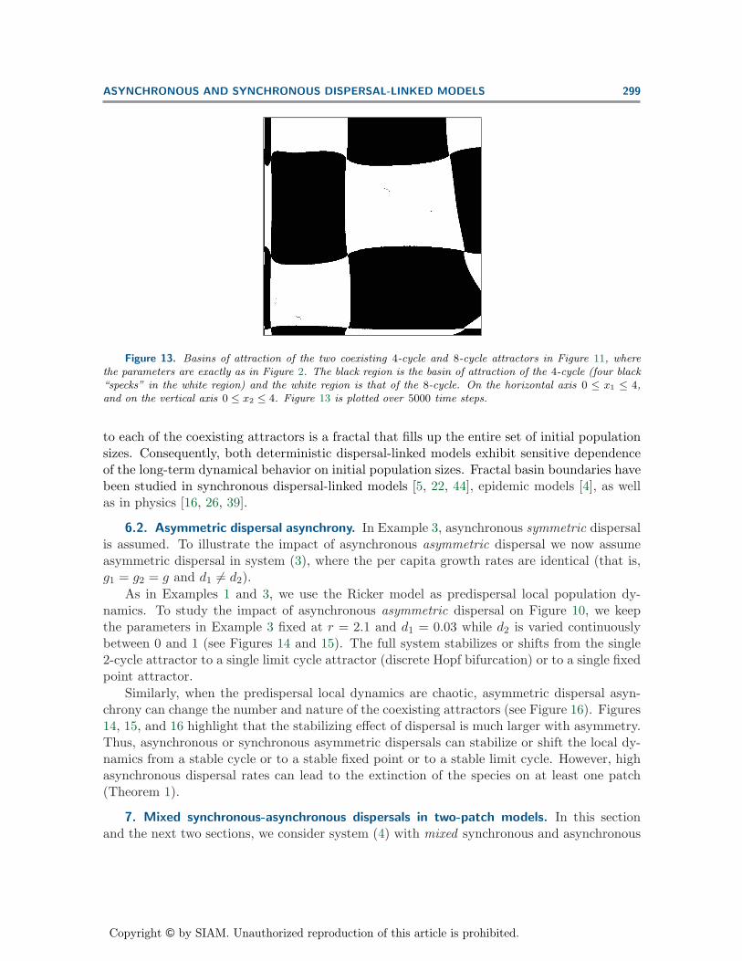
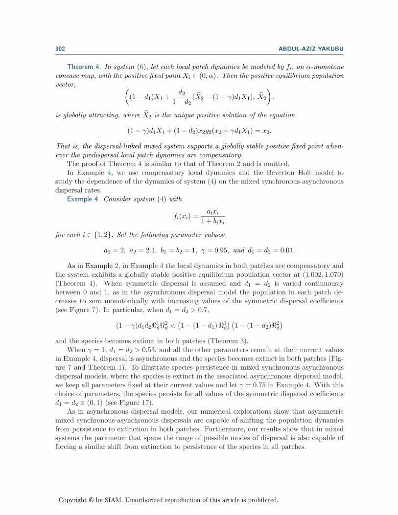
Figure 13. Basins of attraction of the two coexisting 4-cycle and 8-cycle attractors in Figure 11, wherethe parameters are exactly as in Figure 2. The black region is the basin of attraction of the 4-cycle (four black“specks” in the white region) and the white region is that of the 8-cycle. On the horizontal axis 0 ≤ x1 ≤ 4,and on the vertical axis 0 ≤ x2 ≤ 4. Figure 13 is plotted over 5000 time steps.

to each of the coexisting attractors is a fractal that fills up the entire set of initial populationsizes. Consequently, both deterministic dispersal-linked models exhibit sensitive dependenceof the long-term dynamical behavior on initial population sizes. Fractal basin boundaries havebeen studied in synchronous dispersal-linked models [5, 22, 44], epidemic models [4], as wellas in physics [16, 26, 39].

6.2. Asymmetric dispersal asynchrony. In Example 3, asynchronous symmetric dispersalis assumed. To illustrate the impact of asynchronous asymmetric dispersal we now assumeasymmetric dispersal in system (3), where the per capita growth rates are identical (that is,g1 = g2 = g and d1 �= d2).

As in Examples 1 and 3, we use the Ricker model as predispersal local population dy-namics. To study the impact of asynchronous asymmetric dispersal on Figure 10, we keepthe parameters in Example 3 fixed at r = 2.1 and d1 = 0.03 while d2 is varied continuouslybetween 0 and 1 (see Figures 14 and 15). The full system stabilizes or shifts from the single2-cycle attractor to a single limit cycle attractor (discrete Hopf bifurcation) or to a single fixedpoint attractor.

Similarly, when the predispersal local dynamics are chaotic, asymmetric dispersal asyn-chrony can change the number and nature of the coexisting attractors (see Figure 16). Figures14, 15, and 16 highlight that the stabilizing effect of dispersal is much larger with asymmetry.Thus, asynchronous or synchronous asymmetric dispersals can stabilize or shift the local dy-namics from a stable cycle or to a stable fixed point or to a stable limit cycle. However, highasynchronous dispersal rates can lead to the extinction of the species on at least one patch(Theorem 1).

7. Mixed synchronous-asynchronous dispersals in two-patch models. In this sectionand the next two sections, we consider system (4) with mixed synchronous and asynchronous



Figure 14. After period-doubling reversals and Hopf bifurcation, Patch 2 population decreases monotonicallyto zero, while Patch 1 population increases monotonically to a maximum value before decreasing to the Patch 1predispersal 2-cycle dynamics, where r1 = 2.1, d1 = 0.03, and d2 is varied continuously between 0 and 1.

Figure 15. A limit cycle attractor with asymmetric dispersal asynchrony, where r1 = 2.1, d1 = 0.03, andd2 = 0.032.

dispersals (that is, system (4) with 0 < γ < 1). Recall that there is no population explosion insystem (4). Consequently, by regular perturbation analysis at the endpoints γ = 0 and γ = 1,one obtains that when γ is sufficiently small (respectively, large) the qualitative dynamics ofthe dispersal-linked system under mixed synchronous and asynchronous dispersals are similarto that of the corresponding system under only synchronous (respectively, asynchronous)dispersal.

If γ = 0 and dispersal is synchronous (0 < d1, d2 < 1), it is known that the speciesalways persists in both patches, where g1(0), g2(0) > 1 [44]. However, if γ = 1 and dispersal isasynchronous, then the species does not always persist in both patches (Theorem 3). If γ �= 1 in



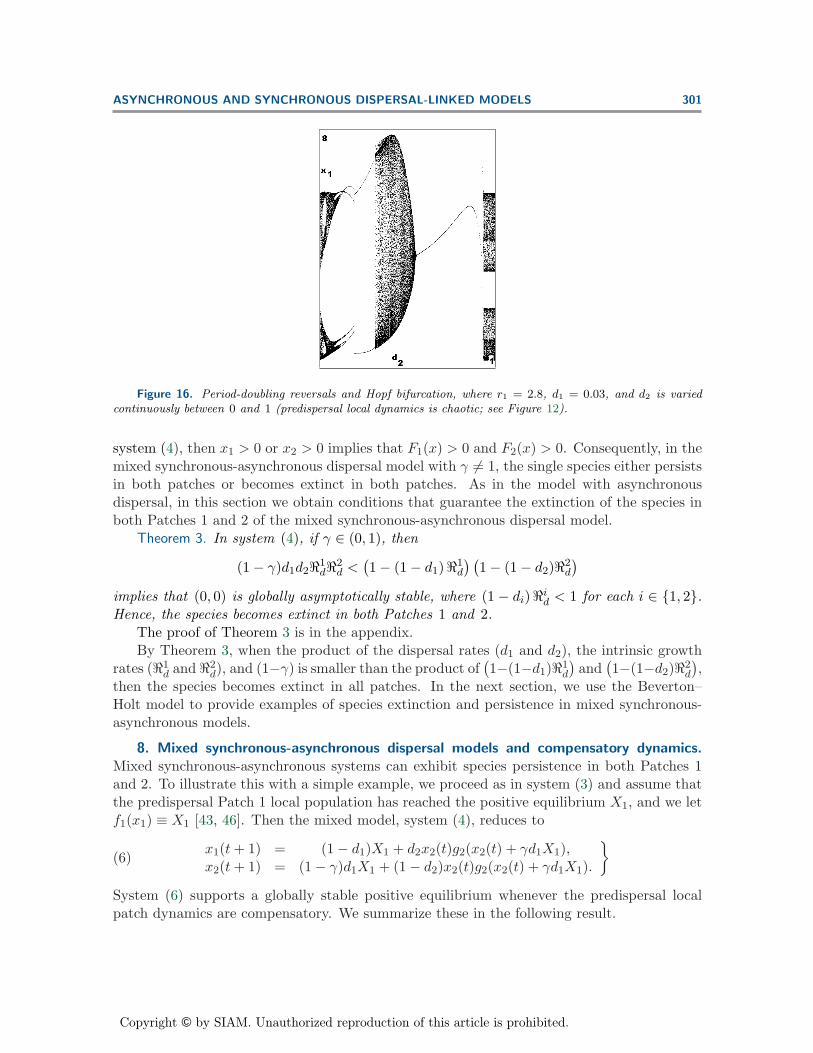
Figure 16. Period-doubling reversals and Hopf bifurcation, where r1 = 2.8, d1 = 0.03, and d2 is variedcontinuously between 0 and 1 (predispersal local dynamics is chaotic; see Figure 12).

system (4), then x1 > 0 or x2 > 0 implies that F1(x) > 0 and F2(x) > 0. Consequently, in themixed synchronous-asynchronous dispersal model with γ �= 1, the single species either persistsin both patches or becomes extinct in both patches. As in the model with asynchronousdispersal, in this section we obtain conditions that guarantee the extinction of the species inboth Patches 1 and 2 of the mixed synchronous-asynchronous dispersal model.

Theorem 3. In system (4), if γ ∈ (0, 1), then

(1 − γ)d1d2�1d�2

d <(1 − (1 − d1)�1

d

) (1 − (1 − d2)�2

d

)implies that (0, 0) is globally asymptotically stable, where (1 − di)�i

d < 1 for each i ∈ {1, 2}.Hence, the species becomes extinct in both Patches 1 and 2.

The proof of Theorem 3 is in the appendix.By Theorem 3, when the product of the dispersal rates (d1 and d2), the intrinsic growth

rates (�1d and �2

d), and (1−γ) is smaller than the product of(1−(1−d1)�1

d

)and

(1−(1−d2)�2

d

),

then the species becomes extinct in all patches. In the next section, we use the Beverton–Holt model to provide examples of species extinction and persistence in mixed synchronous-asynchronous models.

8. Mixed synchronous-asynchronous dispersal models and compensatory dynamics.Mixed synchronous-asynchronous systems can exhibit species persistence in both Patches 1and 2. To illustrate this with a simple example, we proceed as in system (3) and assume thatthe predispersal Patch 1 local population has reached the positive equilibrium X1, and we letf1(x1) ≡ X1 [43, 46]. Then the mixed model, system (4), reduces to

(6)x1(t + 1) = (1 − d1)X1 + d2x2(t)g2(x2(t) + γd1X1),x2(t + 1) = (1 − γ)d1X1 + (1 − d2)x2(t)g2(x2(t) + γd1X1).

}

System (6) supports a globally stable positive equilibrium whenever the predispersal localpatch dynamics are compensatory. We summarize these in the following result.



Theorem 4. In system (6), let each local patch dynamics be modeled by fi, an α-monotoneconcave map, with the positive fixed point Xi ∈ (0, α). Then the positive equilibrium populationvector, (

(1 − d1)X1 +d2

1 − d2(X2 − (1 − γ)d1X1), X2

),

is globally attracting, where X2 is the unique positive solution of the equation

(1 − γ)d1X1 + (1 − d2)x2g2(x2 + γd1X1) = x2.

That is, the dispersal-linked mixed system supports a globally stable positive fixed point when-ever the predispersal local patch dynamics are compensatory.

The proof of Theorem 4 is similar to that of Theorem 2 and is omitted.In Example 4, we use compensatory local dynamics and the Beverton–Holt model to

study the dependence of the dynamics of system (4) on the mixed synchronous-asynchronousdispersal rates.

Example 4. Consider system (4) with

fi(xi) =aixi

1 + bixi


a1 = 2, a2 = 2.1, b1 = b2 = 1, γ = 0.95, and d1 = d2 = 0.01.

As in Example 2, in Example 4 the local dynamics in both patches are compensatory andthe system exhibits a globally stable positive equilibrium population vector at (1.002, 1.070)(Theorem 4). When symmetric dispersal is assumed and d1 = d2 is varied continuouslybetween 0 and 1, as in the asynchronous dispersal model the population in each patch de-creases to zero monotonically with increasing values of the symmetric dispersal coefficients(see Figure 7). In particular, when d1 = d2 > 0.7,

(1 − γ)d1d2�1d�2

d <(1 − (1 − d1)�1

d

) (1 − (1 − d2)�2

d

)and the species becomes extinct in both patches (Theorem 3).

When γ = 1, d1 = d2 > 0.53, and all the other parameters remain at their current valuesin Example 4, dispersal is asynchronous and the species becomes extinct in both patches (Fig-ure 7 and Theorem 1). To illustrate species persistence in mixed synchronous-asynchronousdispersal models, where the species is extinct in the associated asynchronous dispersal model,we keep all parameters fixed at their current values and let γ = 0.75 in Example 4. With thischoice of parameters, the species persists for all values of the symmetric dispersal coefficientsd1 = d2 ∈ (0, 1) (see Figure 17).

As in asynchronous dispersal models, our numerical explorations show that asymmetricmixed synchronous-asynchronous dispersals are capable of shifting the population dynamicsfrom persistence to extinction in both patches. Furthermore, our results show that in mixedsystems the parameter that spans the range of possible modes of dispersal is also capable offorcing a similar shift from extinction to persistence of the species in all patches.



Figure 17. Persistence in both Patches 1 and 2 with symmetric mixed synchronous-asynchronous dispersal,where γ = 0.75, d1 = d2 ∈ (0, 1), and all other parameters remain fixed at their current values in Example 4.

Figure 18. Example 5 has two coexisting 2-cycle attractors for values of γ ∈ [0.0.45) and only a single2-cycle attractor for values of γ ∈ (0.45, 1).

9. Mixed synchronous-asynchronous dispersal models and overcompensatory dynam-ics. The qualitative dynamics of mixed synchronous-asynchronous dispersal systems are simi-lar to those of the associated synchronous (respectively, asynchronous) dispersal systems whenγ, the parameter that spans the range of possible modes of dispersal, is close to 0 (respec-tively, close to 1). In this section, we highlight the possible behaviors of mixed synchronous-asynchronous systems, where the local dynamics are overcompensatory and are governed bythe Ricker model.

Example 5. Consider system (4) with the Ricker model

fi(xi) = xi exp(ri − xi)


r = r1 = r2 = 2.1, γ ∈ [0, 1], and d = d1 = d2 = 0.03.

With our choice of parameters, Example 4 exhibits two coexisting 2-cycle attractors (seeExample 1 and Figures 1 and 18) when γ ∈ [0, 0.45). That is, for these values of the parame-ters, the qualitative dynamics of the system with mixed synchronous-asynchronous dispersals



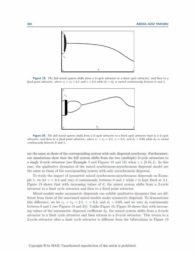
Figure 19. The full mixed system shifts from a 2-cycle attractor to a limit cycle attractor, and then to afixed point attractor, where r1 = r2 = 2.1 and γ = 0.4 while d1 = d2 is varied continuously between 0 and 1.

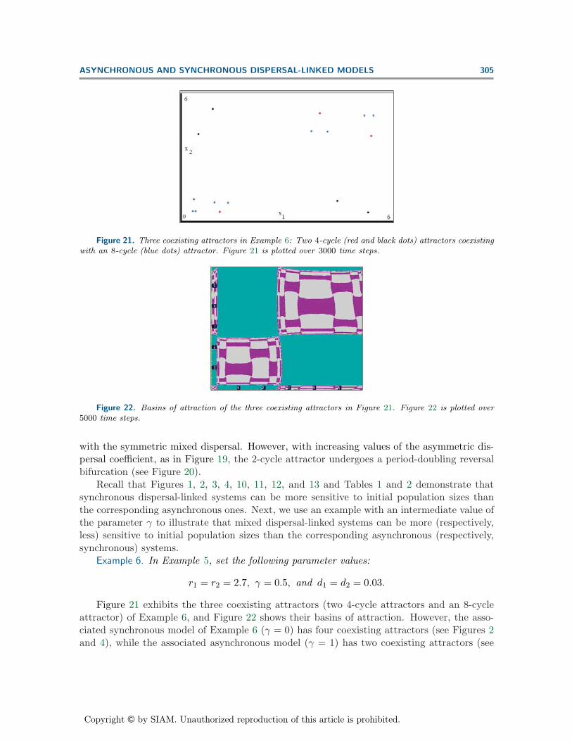
Figure 20. The full mixed system shifts from a 2-cycle attractor to a limit cycle attractor back to a 2-cycleattractor, and then to a fixed point attractor, where r1 = r2 = 2.1, γ = 0.4, and d1 = 0.03 while d2 is variedcontinuously between 0 and 1.

are the same as those of the corresponding system with only dispersal synchrony. Furthermore,our simulations show that the full system shifts from the two (multiple) 2-cycle attractors toa single 2-cycle attractor (see Example 3 and Figures 10 and 18) when γ ∈ [0.45, 1]. In thiscase, the qualitative dynamics of the mixed synchronous-asynchronous dispersal model arethe same as those of the corresponding system with only asynchronous dispersal.

To study the impact of symmetric mixed synchronous-asynchronous dispersals on Exam-ple 5, we let γ = 0.4 and vary d continuously between 0 and 1 while r is kept fixed at 2.1.Figure 19 shows that with increasing values of d, the mixed system shifts from a 2-cycleattractor to a limit cycle attractor and then to a fixed point attractor.

Mixed models under asymmetric dispersals can exhibit qualitative dynamics that are dif-ferent from those of the associated mixed models under symmetric dispersal. To demonstratethis difference, we let r1 = r2 = 2.1, γ = 0.4, and d1 = 0.03, and we vary d2 continuouslybetween 0 and 1 (see Figures 19 and 20). Unlike Figure 19, Figure 20 shows that with increas-ing values of the asymmetric dispersal coefficient d2, the mixed system shifts from a 2-cycleattractor to a limit cycle attractor and then returns to a 2-cycle attractor. This return to a2-cycle attractor after a limit cycle attractor is different from the bifurcations in Figure 19



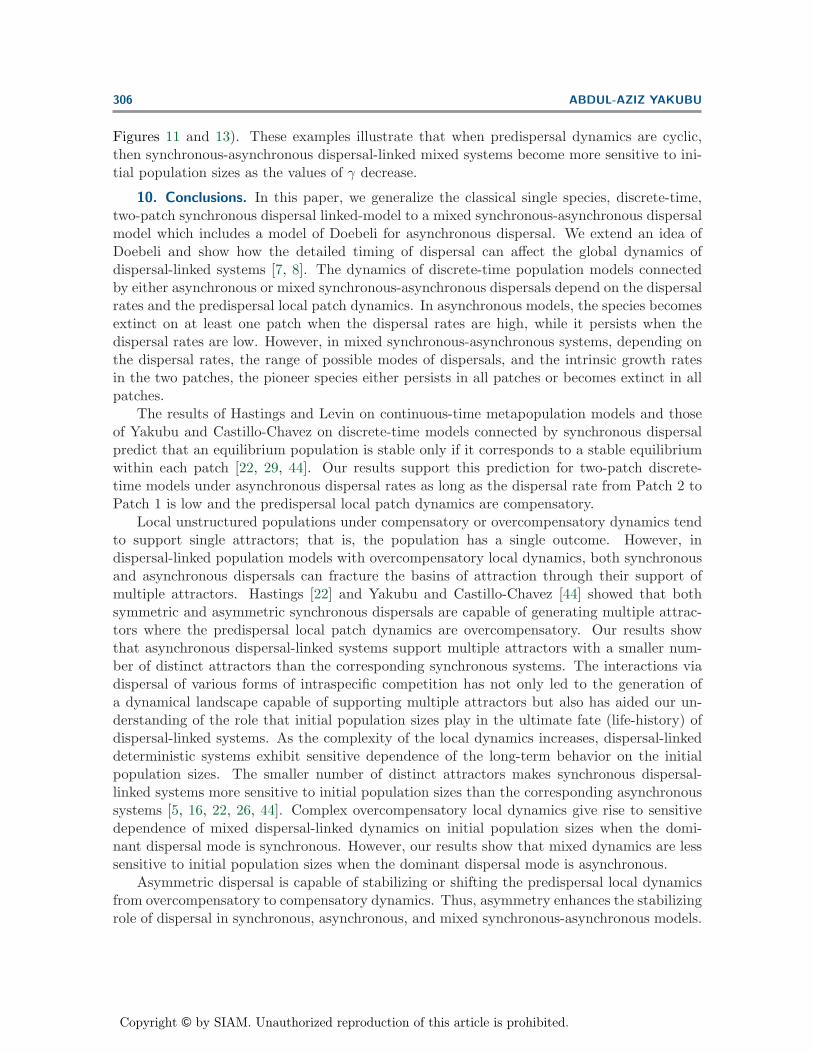
Figure 21. Three coexisting attractors in Example 6: Two 4-cycle (red and black dots) attractors coexistingwith an 8-cycle (blue dots) attractor. Figure 21 is plotted over 3000 time steps.

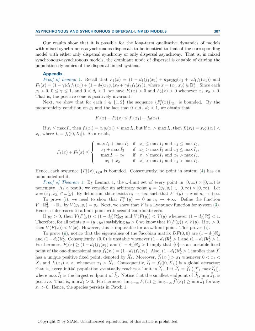
Figure 22. Basins of attraction of the three coexisting attractors in Figure 21. Figure 22 is plotted over5000 time steps.

with the symmetric mixed dispersal. However, with increasing values of the asymmetric dis-persal coefficient, as in Figure 19, the 2-cycle attractor undergoes a period-doubling reversalbifurcation (see Figure 20).

Recall that Figures 1, 2, 3, 4, 10, 11, 12, and 13 and Tables 1 and 2 demonstrate thatsynchronous dispersal-linked systems can be more sensitive to initial population sizes thanthe corresponding asynchronous ones. Next, we use an example with an intermediate value ofthe parameter γ to illustrate that mixed dispersal-linked systems can be more (respectively,less) sensitive to initial population sizes than the corresponding asynchronous (respectively,synchronous) systems.

Example 6. In Example 5, set the following parameter values:

r1 = r2 = 2.7, γ = 0.5, and d1 = d2 = 0.03.

Figure 21 exhibits the three coexisting attractors (two 4-cycle attractors and an 8-cycleattractor) of Example 6, and Figure 22 shows their basins of attraction. However, the asso-ciated synchronous model of Example 6 (γ = 0) has four coexisting attractors (see Figures 2and 4), while the associated asynchronous model (γ = 1) has two coexisting attractors (see



Figures 11 and 13). These examples illustrate that when predispersal dynamics are cyclic,then synchronous-asynchronous dispersal-linked mixed systems become more sensitive to ini-tial population sizes as the values of γ decrease.

10. Conclusions. In this paper, we generalize the classical single species, discrete-time,two-patch synchronous dispersal linked-model to a mixed synchronous-asynchronous dispersalmodel which includes a model of Doebeli for asynchronous dispersal. We extend an idea ofDoebeli and show how the detailed timing of dispersal can affect the global dynamics ofdispersal-linked systems [7, 8]. The dynamics of discrete-time population models connectedby either asynchronous or mixed synchronous-asynchronous dispersals depend on the dispersalrates and the predispersal local patch dynamics. In asynchronous models, the species becomesextinct on at least one patch when the dispersal rates are high, while it persists when thedispersal rates are low. However, in mixed synchronous-asynchronous systems, depending onthe dispersal rates, the range of possible modes of dispersals, and the intrinsic growth ratesin the two patches, the pioneer species either persists in all patches or becomes extinct in allpatches.

The results of Hastings and Levin on continuous-time metapopulation models and thoseof Yakubu and Castillo-Chavez on discrete-time models connected by synchronous dispersalpredict that an equilibrium population is stable only if it corresponds to a stable equilibriumwithin each patch [22, 29, 44]. Our results support this prediction for two-patch discrete-time models under asynchronous dispersal rates as long as the dispersal rate from Patch 2 toPatch 1 is low and the predispersal local patch dynamics are compensatory.

Local unstructured populations under compensatory or overcompensatory dynamics tendto support single attractors; that is, the population has a single outcome. However, indispersal-linked population models with overcompensatory local dynamics, both synchronousand asynchronous dispersals can fracture the basins of attraction through their support ofmultiple attractors. Hastings [22] and Yakubu and Castillo-Chavez [44] showed that bothsymmetric and asymmetric synchronous dispersals are capable of generating multiple attrac-tors where the predispersal local patch dynamics are overcompensatory. Our results showthat asynchronous dispersal-linked systems support multiple attractors with a smaller num-ber of distinct attractors than the corresponding synchronous systems. The interactions viadispersal of various forms of intraspecific competition has not only led to the generation ofa dynamical landscape capable of supporting multiple attractors but also has aided our un-derstanding of the role that initial population sizes play in the ultimate fate (life-history) ofdispersal-linked systems. As the complexity of the local dynamics increases, dispersal-linkeddeterministic systems exhibit sensitive dependence of the long-term behavior on the initialpopulation sizes. The smaller number of distinct attractors makes synchronous dispersal-linked systems more sensitive to initial population sizes than the corresponding asynchronoussystems [5, 16, 22, 26, 44]. Complex overcompensatory local dynamics give rise to sensitivedependence of mixed dispersal-linked dynamics on initial population sizes when the domi-nant dispersal mode is synchronous. However, our results show that mixed dynamics are lesssensitive to initial population sizes when the dominant dispersal mode is asynchronous.

Asymmetric dispersal is capable of stabilizing or shifting the predispersal local dynamicsfrom overcompensatory to compensatory dynamics. Thus, asymmetry enhances the stabilizingrole of dispersal in synchronous, asynchronous, and mixed synchronous-asynchronous models.



Our results show that it is possible for the long-term qualitative dynamics of modelswith mixed synchronous-asynchronous dispersals to be identical to that of the correspondingmodel with either only dispersal synchrony or only dispersal asynchrony. That is, in mixedsynchronous-asynchronous models, the dominant mode of dispersal is capable of driving thepopulation dynamics of the dispersal-linked systems.

Appendix.Proof of Lemma 1. Recall that F1(x) = (1 − d1)f1(x1) + d2x2g2(x2 + γd1f1(x1)) and

F2(x) = (1− γ)d1f1(x1) + (1− d2)x2g2(x2 + γd1f1(x1)), where x = (x1, x2) ∈ R2+. Since each

gi > 0, 0 ≤ γ ≤ 1, and 0 < di < 1, we have F1(x) > 0 and F2(x) > 0 whenever x1, x2 > 0.That is, the positive cone is positively invariant.

Next, we show that for each i ∈ {1, 2} the sequence {F ti (x)}t≥0 is bounded. By the

monotonicity condition on g2 and the fact that 0 < d1, d2 < 1, we obtain that

F1(x) + F2(x) ≤ f1(x1) + f2(x2).

If xi ≤ max Ii, then fi(xi) = xigi(xi) ≤ max Ii, but if xi > max Ii, then fi(xi) = xigi(xi) <xi, where Ii ≡ fi([0, Xi]). As a result,

F1(x) + F2(x) ≤

⎧⎪⎪⎨⎪⎪⎩

max I1 + max I2 if x1 ≤ max I1 and x2 ≤ max I2,x1 + max I2 if x1 > max I1 and x2 ≤ max I2,max I1 + x2 if x1 ≤ max I1 and x2 > max I2,x1 + x2 if x1 > max I1 and x2 > max I2.

Hence, each sequence {F ti (x)}t≥0 is bounded. Consequently, no point in system (4) has an

unbounded orbit.Proof of Theorem 1. By Lemma 1, the ω-limit set of every point in [0,∞) × [0,∞) is

nonempty. As a result, we consider an arbitrary point y = (y1, y2) ∈ [0,∞) × [0,∞). Letx = (x1, x2) ∈ ω(y). By definition, there exists ni → +∞ such that Fni(y) → x as ni → +∞.

To prove (i), we need to show that Fni2 (y) → 0 as ni → +∞. Define the function

V : R2+ → R+ by V (y1, y2) = y2. Next, we show that V is a Lyapunov function for system (3).

Hence, it decreases to a limit point with second coordinate zero.If y2 > 0, then V (F (y)) < (1 − d2)�2

dy2 and V (F (y)) < V (y) whenever (1 − d2)�2d < 1.

Therefore, for all points y = (y1, y2) satisfying y2 > 0 we know that V (F (y)) < V (y). If x2 > 0,then V (F (x)) < V (x). However, this is impossible for an ω-limit point. This proves (i).

To prove (ii), notice that the eigenvalues of the Jacobian matrix DF (0, 0) are (1 − d1)�1d

and (1− d2)�2d. Consequently, (0, 0) is unstable whenever (1− d1)�1

d > 1 and (1− d2)�2d > 1.

Furthermore, F1(x) ≥ (1 − d1)f1(x1) and (1 − d1)�1d > 1 imply that {0} is an unstable fixed

point of the one-dimensional map f1(x1) = (1−d1)f1(x1). Also, (1−d1)�1d > 1 implies that f1

has a unique positive fixed point, denoted by X1. Moreover, f1(x1) > x1 whenever 0 < x1 <X1 and f1(x1) < x1 whenever x1 > X1. Consequently, I1 ≡ f1([0, X1]) is a global attractor;

that is, every initial population eventually reaches a limit in I1. Let J1 ≡ f1

([X1,max I1]

),

where max I1 is the largest endpoint of I1. Notice that the smallest endpoint of J1, min J1, is

positive. That is, min J1 > 0. Furthermore, limt→∞ F t1(x) ≥ limt→∞ f t

1(x1) ≥ min J1 for anyx1 > 0. Hence, the species persists in Patch 1.



To prove (iii) and (iv), notice that when Patch 2 is empty (that is, when (1− d2)�2d < 1),

the Patch 1 population is governed by the “limiting equation” F1(x) = (1 − d1)f1(x1). ThatPatch 1 dynamics are compensatory implies that (0, 0) is globally stable when �d < 1, while(0, 0) is unstable and (g−1

1 ( 11−d1

), 0) is globally stable when (1−d1)�1d > 1 and (1−d2)�2

d < 1.This completes the proof.

The following result is useful in the proof of Theorem 2.Lemma 2. Let f2(x2) = (1 − d2)x2g2(x2 + d1X1). If Patch 2 dynamics are compensatory

and (1 − d2)�2d > 1, then f2 is orientation-preserving and all positive densities approach the

positive equilibrium at X2 = g−12 ( 1

1−d2) − d1X1 monotonically under f2 iterations.

Proof of Lemma 2. First, notice that (1− d2)�2d > 1 implies that f2 has a unique positive

fixed point at X2. To prove the result, we need to show that X2 is globally stable in (0,∞). If

we know that f2 cannot support 2-cycles, then Sharkovskii’s theorem implies that f2 cannothave cycles except for a fixed point. Using the monotonicity condition on g2 and the fact thatX2 > 0, we obtain that zero and infinity are repellors under f2 iterations. Since no pointovershoots X2, we obtain that the unique positive fixed point of f2, X2 is globally stable in(0,∞) and no point overshoots it under f2 iterations.

Now, we prove that f2 cannot support 2-cycles. Suppose that f2 has a 2-cycle. SincePatch 2 predispersal local dynamics are compensatory and (1 − d2)�2

d > 1, we have that the

fixed point X2 must be unstable and (f2)′(X2) < −1. That is, (f2)

′(X2) = (1− d1)(g2(X2) +

X2g′2(X2)) < −1. Since gi(Xi) = 1 and X2 = X2 − d1X1, we have

(1 − d1)f′2(X2) = (1 − d1)(1 + X2g

′2(X2))

≤ (1 − d1)(1 + (X2 + d1X1)g′2(X2)) < −1 + (1 − d1)d1X1g

′2(X2) < 0.

This contradicts the fact that (1 − d1)f′2(X2) > 0 (compensatory dynamics). As a result, f2

cannot support 2-cycles. This establishes Lemma 2.Proof of Theorem 2. Notice that system (4) is essentially a one-dimensional system. By

Lemma 2, limt→∞ F t2(x) = (g−1

2 ( 11−d2

) − d1X1) for each point x = (x1, x2) ∈ (0,∞) × (0,∞).

Consequently, limt→∞ F t1(x) = (1 − d1)X1 + d2

1−d2(g−1

2 ( 11−d2

) − d1X1), and the positive fixedpoint is globally asymptotically stable in (0,∞) × (0,∞).

Proof of Theorem 3. To prove Theorem 3, we proceed as in the proof of Theorem 1 anddefine the function V : R

2+ → R+ by

V (y1, y2) = y1 + by2,

where

0 <d2�2

d

1 − (1 − d2)�2d

< b <1 − (1 − d1)�1

d

(1 − γ)d1�1d

.

Next, we show that V is a Lyapunov function for system (4), where γ �= 0, 1. Hence, itdecreases to a limit point with both coordinates equal to zero.

V (F (y)) = ((1 − d1) + (1 − γ)bd1) f1(y1) + (d2 + b(1 − d2))y2g2(y2 + γd1f1(y1)). If y =(y1, y2) �= (0, 0), then

V (F (y)) < ((1 − d1) + (1 − γ)bd1)�1dy1 + (d2 + b(1 − d2))�2

dy2.



With our choice of the positive constant b, we have

((1 − d1) + (1 − γ)bd1)�1d < 1

and(d2 + b(1 − d2))�2

d < b.

Hence V (F (y)) < V (y) whenever 0 <d2�2

d

1−(1−d2)�2d<

1−(1−d1)�1d

(1−γ)d1�1d

. Therefore, for all points

y = (y1, y2) �= (0, 0) we know that V (F (y)) < V (y). Now, proceed exactly as in the proof ofTheorem 1 to complete the proof.

Acknowledgment. The author thanks the referees for their useful suggestions.

REFERENCES

[1] L. J. Allen, Persistence, extinction, and critical patch number for island populations, J. Math. Biol., 24(1987), pp. 617–625.

[2] M. Begon, J. L. Harper, and C. R. Townsend, Ecology: Individuals, Populations and Communities,Blackwell Science, Malden, MA, 1996.

[3] F. Brauer and C. Castillo-Chavez, Mathematical Models in Population Biology and Epidemiology,Texts Appl. Math. 40, Springer-Verlag, New York, 2001.

[4] C. Castillo-Chavez and A. A. Yakubu, Dispersal, disease and life-history evolution, Math. Biosci.,173 (2001), pp. 35–53.

[5] C. Castillo-Chavez and A. A. Yakubu, Intraspecific competition, dispersal and disease dynamicsin discrete-time patchy environments, in Mathematical Approaches for Emerging and ReemergingInfectious Diseases: An Introduction to Models, Methods and Theory, C. Castillo-Chavez, S. Blower,P. van den Driessche, D. Kirschner, and A.-A. Yakubu, eds., Springer-Verlag, New York, 2001, pp.165–181.

[6] D. Cohen and S. A. Levin, The interaction between dispersal and dormancy strategies in varyingand heterogeneous environments, in Mathematical Topics in Population Biology, Morphogenesis andNeurosciences, E. Teramoto and M. Yamaguti, eds., Springer-Verlag, Berlin, 1987, pp. 110–122.

[7] M. Doebeli, Dispersal and dynamics, Theoret. Population Biol., 47 (1995), pp. 82–106.[8] M. Doebeli and G. D. Ruxton, Evolution of dispersal rates in metapopulation model: Branching and

cyclic dynamics in phenotype space, Evolution, 5 (1997), pp. 1730–1741.[9] D. J. Earn, S. A. Levin, and P. Rohani, Coherence and conservation, Science, 290 (2000), pp. 1360–

1364.[10] P. L. Errington, Some contributions of a fifteen year local study of the northern bobwhite to a knowledge

of population phenomena, Ecol. Monogr., 15 (1945), pp. 1–34.[11] J. E. Franke and A.-A. Yakubu, Extinction and persistence of species in discrete competitive systems

with a safe refuge, J. Math. Anal. Appl., 23 (1996), pp. 746–761.[12] J. E. Franke and A.-A. Yakubu, Geometry of exclusion principles in discrete systems, J. Math. Anal.

Appl., 168 (1992), pp. 385–400.[13] J. E. Franke and A.-A. Yakubu, Mutual exclusion versus coexistence for discrete competitive systems,

J. Math. Biol., 30 (1991), pp. 161–168.[14] M. Gadgil, Dispersal: Population consequences and evolution, Ecology, 52 (1971), pp. 253–261.[15] J. L. Gonzalez-Andujar and J. N. Perry, Chaos, metapopulations and dispersal, Ecol. Model., 65

(1993), pp. 255–263.[16] C. Grebogi, E. Ott, and J. A. Yorke, Chaos, strange attractors, and fractal basin boundaries in

nonlinear dynamics, Science, 228 (1987), pp. 632–638.[17] M. Gyllenberg, G. Soderbacka, and S. Ericsson, Does migration stabilize local population dynam-

ics? Analysis of a discrete metapopulation model, Math. Biosci., 118 (1993), pp. 25–49.[18] I. Hanski, Single-species metapopulation dynamics: Concepts, models and observations, Biol. J. Linn.

Soc., 42 (1991), pp. 17–38.



[19] I. A. Hanski and M. E. Gilpin, Metapopulation Biology: Ecology, Genetics, and Evolution, AcademicPress, San Diego, 1997.

[20] M. P. Hassell, The Dynamics of Competition and Predation, Studies in Biol. 72, Edward Arnold,London, 1976.

[21] M. P. Hassell, J. H. Lawton, and R. M. May, Patterns of dynamical behavior in single speciespopulations, J. Anim. Ecol., 45 (1976), pp. 471–486.

[22] A. Hastings, Complex interactions between dispersal and dynamics: Lessons from coupled logistic equa-tions, Ecology, 75 (1993), pp. 1362–1372.

[23] A. Hastings, Dynamics of a single species in a spatially varying environment: The stabilizing role ofhigh dispersal rates, J. Math. Biol., 16 (1982), pp. 49–55.

[24] S. M. Henson, R. F. Constantino, J. M. Cushing, B. Dennis, and R. A. Desharnais, Multipleattractors, saddles, and population dynamics in periodic habitats, Bull. Math. Biol., 61 (1999), pp.1121–1149.

[25] S. M. Henson and J. M. Cushing, Hierarchical models of intraspecific competition: Scramble versuscontest, J. Math. Biol., 34 (1996), pp. 755–772.

[26] I. Kan, Open sets of diffeomorphisms having two attractors, each with an everywhere dense basin, Bull.Amer. Math. Soc. (N.S.), 31 (1994), pp. 68–74.

[27] S. A. Levin, Dispersion and population interactions, Amer. Naturalist, 108 (1974), pp. 207–228.[28] S. A. Levin, The problem of pattern and scale in ecology, Ecology, 73 (1992), pp. 1943–1967.[29] S. Levin and R. T. Paine, Disturbance, patch formation, and community structure, Proc. Nat. Acad.

Sci. USA, 68 (1974), pp. 2744–2747.[30] R. Levins, Some demographic and genetic consequences of environmental heterogeneity for biological

control, Bull. Entomol. Soc. Amer., 15 (1969), pp. 237–240.[31] R. Levins, The effect of random variation of different types on population growth, Proc. Nat. Acad. Sci.

USA, 62 (1969), pp. 1061–1062.[32] R. M. May and G. F. Oster, Bifurcations and dynamic complexity in simple ecological models, Amer.

Naturalist, 110 (1976), pp. 573–579.[33] R. M. May, Simple mathematical models with very complicated dynamics, Nature, 261 (1977), pp. 459–

469.[34] R. M. May, Stability and Complexity in Model Ecosystems, Princeton University Press, Princeton, NJ,

1974.[35] R. M. May, M. P. Hassell, R. M. Anderson, and D. W. Tonkyn, Density dependence in host-

parasitoid models, J. Anim. Ecol., 50 (1981), pp. 855–865.[36] J. Maynard Smith and M. Slatkin, The stability of predator-prey systems, Ecology, 54 (1973), pp.

384–391.[37] J. G. Milton and J. Belair, Chaos, noise, and extinction in models of population growth, Theoret.

Population Biol., 37 (1990), pp. 273–290.[38] A. J. Nicholson, Compensatory reactions of populations to stresses, and their evolutionary significance,

Aust. J. Zool., 2 (1954), pp. 1–65.[39] H. E. Nusse and J. A. Yorke, Dynamics: Numerical Explorations, Springer-Verlag, New York, 1997.[40] W. E. Ricker, Stock and recruitment, J. Fisheries Research Board of Canada, 11 (1954), pp. 559–623.[41] T. Royama, Analytical Population Dynamics, Pop & Comm. Biol. Series 10, Chapman & Hall, Boca

Raton, FL, 1992.[42] H. L. Smith, Cooperative systems of differential equations with concave nonlinearities, Nonlinear Anal.,

10 (1986), pp. 1037–1052.[43] H. R. Thieme, Convergence results and a Poincare-Bendixson trichotomy for asymptotically autonomous

differential equations, J. Math. Biol., 30 (1992), pp. 755–763.[44] A. Yakubu and C. Castillo-Chavez, Interplay between local dynamics and dispersal in discrete-time

metapopulation models, J. Theoret. Biol., 218 (2002), pp. 273–288.[45] P. Yodzis, Introduction to Theoretical Ecology, Harper & Row, New York, 1989.[46] X.-Q. Zhao, Asymptotic behavior for asymptotically periodic semiflows with applications, Comm. Appl.

Nonlinear Anal., 3 (1996), pp. 43–66.

asynchronous and synchronous dispersals in spatially...

Documents