arX

iv:a

stro

-ph/

0610

949v

1 3

1 O

ct 2

006

Draft version September 3, 2018Preprint typeset using LATEX style emulateapj v. 02/09/03

MAGNETIZED NON-LINEAR THIN SHELL INSTABILITY: NUMERICAL STUDIES IN 2D

Fabian Heitsch1, Adrianne D. Slyz2,3, Julien E.G. Devriendt2, Lee W. Hartmann1, and Andreas Burkert4

Draft version September 3, 2018

ABSTRACT

We revisit the analysis of the Non-linear Thin Shell Instability (NTSI) numerically, including magneticfields. The magnetic tension force is expected to work against the main driver of the NTSI – namelytransverse momentum transport. However, depending on the field strength and orientation, theinstability may grow. For fields aligned with the inflow, we find that the NTSI is suppressed onlywhen the Alfven speed surpasses the (supersonic) velocities generated along the collision interface.Even for fields perpendicular to the inflow, which are the most effective at preventing the NTSIfrom developing, internal structures form within the expanding slab interface, probably leading tofragmentation in the presence of self-gravity or thermal instabilities. High Reynolds numbers resultin local turbulence within the perturbed slab, which in turn triggers reconnection and dissipation ofthe excess magnetic flux. We find that when the magnetic field is initially aligned with the flow, thereexists a (weak) correlation between field strength and gas density. However, for transverse fields, thiscorrelation essentially vanishes. In light of these results, our general conclusion is that instabilities areunlikely to be erased unless the magnetic energy in clouds is much larger than the turbulent energy.Finally, while our study is motivated by the scenario of molecular cloud formation in colliding flows,our results span a larger range of applicability, from supernovae shells to colliding stellar winds.Subject headings: instabilities — MHD — turbulence — methods:numerical — ISM:clouds — ISM:

magnetic fields

1. motivation

Shocks and shells exist abundantly in the interstel-lar medium (ISM). Driven by supernovae, expandingHII-regions, gravitational flows or wholesale cloud col-lisions, they not only strongly influence the ISM dy-namics, but also affect its chemistry. However, struc-tural analyses of the ISM show spectral indices closerto the Kolmogorov value of incompressible turbulence(see Elmegreen & Scalo 2004 for a review). Indepen-dently of the problem of how well these indices con-strain the type of turbulence, there are plenty of physicalmechanisms to explain the closeness to the Kolmogorovvalue, ranging from the intrinsic nature of MHD tur-bulence (e.g. Goldreich & Sridhar 1995, Boldyrev et al.2002, Cho & Lazarian 2003) to the conversion of com-pressible to solenoidal modes (Falgarone et al. 1994,Elmegreen & Scalo 2004).It is the latter mechanism that motivated this study.

In the absence of shear flows (oblique shocks) and ther-mal instabilities, the Non-linear Thin Shell Instability(Vishniac 1994) provides a natural mechanism to convertcompressible motions into solenoidal ones. The NTSI isa rippling instability, relying on transverse momentumtransport due to bends in the collision interface of twoopposing flows. It is likely to arise in a wide range of envi-ronments, from colliding stellar winds, supernova shells,colliding HI streams/clouds, to galaxy mergers.

1 Dept. of Astronomy, University of Michigan, 500 Church St.,Ann Arbor, MI 48109-1042, U.S.A

2 Universite Claude Bernard Lyon 1, CRAL, Observatoire deLyon, 9 Avenue Charles Andre, 69561 St-Genis Laval Cedex,France; CNRS, UMR 5574; ENS Lyon

3 Oxford University, Astrophysics, Denys Wilkinson Building,Keble Road, Oxford, OX1 3RH, United Kingdom

4 University Observatory Munich, Scheinerstr. 1, 81679 Munich,Germany

The NTSI has been widely studied numerically (seeHeitsch et al. 2006 for a summary of the literature),mostly focusing on the effects of self-gravity and ther-mal instabilities. Our interest in the NTSI comesfrom the role it plays in the evolution of molecu-lar clouds in colliding HI flows (Heitsch et al. 2005,2006; Vazquez-Semadeni et al. 2006), but the resultshave a wider applicability. With the exception ofKlein & Woods (1998), who included the magnetic pres-sure term in their study of cloud collisions, work onthe NTSI has so far neglected the effect of magneticfields. However, fields could have a deciding influenceon the evolution of a shock-bounded slab. Motivated bythe numerical models of Vazquez-Semadeni et al. (1995)and Passot et al. (1995), Hartmann et al. (2001) andBergin et al. (2004) suggested that fields could, in fact,lead to a selection effect for molecular cloud formation:clouds can only form if the fields are aligned with theflows assembling the gas.As a first step, we revisit the isothermal analysis of

Vishniac (1994) numerically, and study the evolution ofthe NTSI in a two-dimensional, magnetohydrodynami-cal environment. While the general expectation (§2 2.1)is met in the laminar case, namely that magnetic fieldscan efficiently damp the NTSI, the geometry of the rip-pled interface induces non-ideal MHD effects, requiringa numerical method capable of handling such effects in astable and accurate way (§2 2.2). However, we find thatthe exact amount of dampening crucially depends on thefield orientation and strength (§3). This is especially truein the turbulent case, where turbulent reconnection in-side the over-pressured slab leads to a pressure deficit,thus compressing the gas even further. Finally, we showthat the correlation between field strength and gas den-sity is at best weak, even in the case of fields perpendic-ularly oriented with respect to the inflow, for which the

2 Magnetized NTSI in 2D

field would be expected to scale linearly with the density.

2. physics and numerics

2.1. Physics

The growth rate of the NTSI is mostly controlled by kη,the product of the wave number of the slab perturbationk, and the amplitude of the slab’s initial displacementη (equivalently, the amplitude of the collision interface’sgeometrical perturbation). The instability is driven bylateral transport of longitudinal momentum, i.e. if theinflow is parallel to the x direction, and the slab is in they-z-plane, x-momentum is transported laterally in y (andz), collecting at the focal points of the perturbed slab.The efficiency of lateral momentum transport is key tothe development of the instability, since it is the imbal-ance of ram pressure at the focal points that eventuallypropels matter forward, driving the growth of the slab’sperturbation. Vishniac (1994) derived a growth rate of

ω ≈ csk(kη)1/2, (1)

with the sound speed cs. Blondin & Marks (1996) foundthat at constant η and for small ks, equation (1) yieldsonly a lower limit, while for large ks, the analyticalgrowth rates agree well with the numerical results. Thereason for this seems to lie in the efficiency of deflectingthe incoming flow: for small ks, a small fraction of theincoming flow’s momentum is converted to lateral mo-tions, while a large part compresses the slab (dependingon the equation of state, this could lead to an increasein energy losses).After the initial growth-phase (eq. [1]), the NTSI

reaches saturation through two mechanisms: (i) expan-sion of the slab which stops the lateral momentum trans-port by preventing the inflow from reaching the focalpoints, and (ii) shear flow (Kelvin-Helmholtz) instabil-ities (KHI) in regions of the slab connecting the focalpoints. The KHIs both generate inner structure and re-vive the slab’s expansion. Note that strong cooling (notmodeled here) can also suppress the NTSI via early frag-mentation (Hueckstaedt 2003).Qualitatively, we expect magnetic fields to prevent the

NTSI and subsequent KHI-modes from occurring. How-ever, the detailed quantitative extent of the dampingshould depend on the orientation of the field with respectto the inflow. Indeed, fields aligned with the inflow resistinstabilities via the magnetic tension force, and thereforeshould be more efficient in suppressing the NTSI whenkη is small, even though the strong pairwise field rever-sals arising from the opposed shear velocities along theslab (see §3 3.1) could trigger reconnection. On the otherhand, fields perpendicular to the inflow (but still in the2D plane), primarily prevent instabilities from growingbecause of the magnetic pressure term in the Lorentzforce, and to a lesser extent, because of magnetic tension.For the sake of completeness, we mention that the thirdpossible field configuration in 2D, i.e. the one in whichthe magnetic field is perpendicular to the flow plane, isirrelevant for this study since in that case the gas behavesas a system with an adiabatic exponent of 2 for whichthe NTSI cannot be excited (Vishniac 1994).

2.2. Numerics

The magnetohydrodynamical scheme5 is based ona conservative gas-kinetic flux-splitting method, intro-duced by Xu (1999) and Tang & Xu (2000) and derivedfrom the 1st-order BGK (Bhatnagar et al. 1954) model.Representing the velocity distributions as Maxwelliansin each cell, fluxes across cell walls are derived from thedifferences in the velocity moments of Maxwellian distri-butions reconstructed at the cell walls. The reconstruc-tion is second order in space using MUSCL limiters, andit allows a fast and consistent way to implement vis-cosity and Ohmic resistivity in the form of dissipativefluxes (Heitsch et al. 2004) at close to zero extra com-puting cost, while preserving the time order of PRO-TEUS since the dissipative terms are not simply added assource terms but are part of the flux computation. Thisallows us to control dissipation in a physical manner,without having to rely on numerical dissipation to ter-minate the turbulent cascade at grid scale. Total energyis conserved at machine-accuracy level for an adiabaticequation of state. In the isothermal version which weare using in §3, the total energy equation is not evolved.PROTEUS uses a 2nd order TVD Runge-Kutta timestepping (Shu & Osher 1988) for the MHD equations toachieve 2nd order temporal accuracy. Fluxes are up-dated in time-unsplit fashion, i.e. flux updates for spa-tial directions are computed using the initial conditionsof the current time step. In order to keep ∇ · B = 0,PROTEUS employs a Hodge projection (Balsara 1998;Zachary et al. 1994). The code is fully message passinginterface (MPI) parallelized.With PROTEUS, one may switch between the MHD-

solver previously described and a purely hydrodynamicalsolver based on the 2nd-order BGK model. The latterimplementation has been introduced and extensively dis-cussed by Prendergast & Xu (1993), Slyz & Prendergast(1999), Heitsch et al. (2006) and Slyz et al. (2006), andwe therefore refer the reader interested in implementa-tion details to these papers.One-dimensional shock tests and the Orszag-Tang vor-

tex have already been discussed by Tang & Xu (2000),hence in what follows, we focus on three other MHD testcases. The two first ones, i.e. the propagation of a linearAlfven wave under resistive damping (§2 2.2 2.2.1) andthe current sheet evolution (§2 2.2 2.2.2) are both meantto test the resistive fluxes, while the third one, i.e. theadvection of a field loop (§2 2.2 2.2.3) is a geometry test.A detailed study of the magnetized Kelvin-Helmholtz In-stability is under way (Palotti et al. 2006).

2.2.1. Propagation of a linear Alfven Wave

This one-dimensional test checks the resistive fluximplementation as well as the accuracy of the overallscheme. A linear Alfven wave under weak Ohmic dissi-pation is damped at a rate of

ωi =1

2λΩk

2, (2)

5 We called the scheme PROTEUS, under which name we willrefer to it subsequently. Proteus is a lesser god in Greek mythology,also known as ”The Old Man of the Sea”. He lives in the sea off thecoast of Egypt and can see things in the past, presence and future,but is very unwilling to share his knowledge. In order to evadequestions, he has the ability to change his appearance. However, ifyou manage to catch and hold him, he will assume his true shapeand answer your questions.

Heitsch et al. 3

Fig. 1.— Damping rate (eq. [2]) of a linear Alfven wave againstOhmic resistivity for κ = 1, 2, 4. The resolution is N = 64. Errorsof the measured damping rates are smaller than the symbol sizes.Lines denote the analytical solution.

where λΩ is the Ohmic resistivity, and k = 2πκ/L isthe wave number of the Alfven wave, with κ ∈ N. Thestrongly damped case, where the decay dominates thetime evolution, is physically uninteresting for our appli-cation, since the Ohmic resistivity is mainly used to con-trol numerical dissipation. Figure 1 shows the dampingrate against Ohmic resistivity λΩ for κ = 1, 2, 4 at a gridresolution of N = 64.From Figure 1, it is clear that, as one diminishes the

value of λΩ, there comes a point when the numerical re-sistivity of the scheme becomes comparable to the phys-ical one, causing the measured damping rate to flattenout and depart from the analytical solution. For κ = 4and λΩ = 0.1, the wave decays too quickly to allow a re-liable measurement, and the system enters the stronglydamped branch of the dispersion relation. However, weemphasize that, even for this high value of κ in lightof the modest resolution we used, the resistivity rangeavailable to PROTEUS spans three orders of magnitude.

2.2.2. Current Sheet

This test is taken from Hawley & Stone (1995) andthe ATHENA test suite6. A square domain of extent−0.5 ≤ x, y ≤ 0.5 and of constant density n0 = 1 andpressure p0 is permeated by a magnetic field along they direction such that By(|x| < 0.25) =

√4π, and By =

−√4π elsewhere. This results in two magnetic null lines,

which then are perturbed by velocities vx = A sin(2πy).The goal is to find the pressure p0 and velocity amplitudeA for which the code crashes. The main problem is –especially in conservative schemes – that the resistivedecay of the field leads to strong localized heating thatin turn generates strong magnetosonic waves. Thus, thesmaller p0 and/or the larger A, the harder the test. Wechose p0 = 0.1 and A = 0.3 fairly close to the “standard”values quoted on the ATHENA web site6, p0 = 0.05 andA = 0.1. Here, we use an adiabatic exponent of γ = 5/3and employ the conservative formulation of the scheme.

6 http://www.astro.princeton.edu/∼jstone/tests/field-loop/Field-loop.html

Fig. 2.— Total magnetic energy against time for the currentsheet test. A finite resistivity λΩ helps stabilize the code.

The test turns out to be very hard for PROTEUS,because of its low numerical diffusivity. Figure 2 sum-marizes the test results in the form of the total magneticenergy against time. The energy evolution splits intotwo branches: one corresponding to the lower-resolutionmodels at all resistivities, and the other representing thehigher-resolution models at λΩ = 0 and λΩ = 10−5. AtλΩ = 10−4, the field decay has converged: both resolu-tions give the same curve. At N = 2562 and λΩ = 0, thecode crashes around t = 6. All other models run up tot = 10 and further.The result confirms the discussion by Tang & Xu

(2000), namely that while the conservative gas-kineticflux splitting method in the BGK-formalism performswell for high-β plasmas (with β defined as the ratio ofthermal over magnetic pressure), it might not be themethod of choice for low-β plasmas, i.e. magneticallydominated systems. Note, however, that this is mainlya consequence of the scheme’s conservative formulation.We experimented with a non-conservative version (i.e.just evolving the internal energy instead of the total en-ergy), which was stable for lower p0 and higher A, albeitat the cost of a less accurate total energy evolution.

2.2.3. Advection of a Field Loop

A cylindrical current distribution (i.e. a fieldloop) is advected diagonally across the simulation do-main. We follow the implementation presented byGardiner & Stone (2005) and the ATHENA test suite6,based on an earlier version by Toth & Odstrcil (1996).Density and pressure are both initially uniform at n0 = 1and p = 1, and the fluid is described as an ideal gaswith an adiabatic exponent of γ = 5/3. The square gridranges from −0.5 ≤ x ≤ 0.5, and the loop is advected atan angle of 30 degrees with respect to the x-axis. Thus,two round trips in x correspond to one crossing in y. Theamplitude of the field loop is set to values 10−3, 10−2 and10−1, with an initial radius of R0 = 0.3. Figure 3 showsthe initial current distribution with the magnetic fieldvectors over-plotted (left), and the final current distribu-tion after two time-units measured in horizontal crossingtimes. The overall shape is preserved, although some ar-tifacts are visible at the upper rim of the loop. These

4 Magnetized NTSI in 2D

Fig. 3.— Current density for field loop advection test (see§2 2.2 2.2.3). Left: Initial condition. Right: After two horizontalcrossings. The grid resolution is 2562.

Fig. 4.— Normalized magnetic energy against time (in unitsof horizontal crossing time), for two resolutions and three fieldstrengths. The highest amplitude leads to waves when perturbedby advection. At a resolution of 1282, the magnetic energy hasdecayed by 3.3% after two crossing times. The fit decay times τare indicated for each model.

results concerning the shape are qualitatively similar tothose posted on the above mentioned website. Note thatwe show the current density, since the artifacts do notshow up in the magnetic energy. This test uses λΩ ≡ 0.Figure 4 presents a quantitative diagnostic of the be-

havior of the code as it tracks the magnetic energy de-cay against the simulation time, in units of horizon-tal crossing times. The initial energy is normalized toone. Line styles denote different amplitudes of the fieldstrength. The solid lines correspond to the case given byGardiner & Stone (2005), the dashed and dash-dottedlines denote cases with larger amplitudes. At an ampli-tude of A = 10−3 and a resolution of 1282, the magneticenergy decays by 3.3% over two horizontal crossing times.The ATHENA website6 quotes a decay of 3.5% with a256x148 grid, using a Roe solver and 3rd order recon-struction.In summary, these numerical test cases demonstrate

that PROTEUS models dissipative MHD effects accu-rately, due to a low intrinsic numerical diffusivity thatcompares well with that of higher-order Godunov meth-ods. Furthermore, it can advect geometrically complexmagnetic field patterns properly, and is well suited in itsenergy conserving form to model MHD flows with β > 1.

2.3. Initial Conditions

To remain as close as possible to Vishniac (1994), wewill use the isothermal version of PROTEUS in the fol-lowing. The initial conditions are similar to those dis-cussed in Heitsch et al. (2005, 2006). Two uniform, iden-tical flows in the x-y computational plane initially collidehead-on at a sinusoidal interface with given wave num-ber ky and amplitude η. The field is either aligned orperpendicular to the inflow, but in both cases in the x-y plane. For the standard runs, we used a rectangulargrid with an extent of 88 pc in x and 44 pc in y. Fieldstrength as well as viscosity and resistivity are varied.The grid resolution varies between Nx ×Ny = 256× 128and 2048× 1024 by factors of 2 in linear resolution. Theisothermal sound speed is cS = 5.3 km s−1, the Machnumber of the instreaming gas is M = 4, and the inflowdensity is set to n0 = 1 cm−3. Thus, in the code unitsystem, the Alfven speed in the inflow region is given bycA = B, the magnetic field strength.

3. results

We give a rough estimate for the field strength requiredto prevent the excitation of the NTSI in §3 3.1. The mor-phology of the instability naturally depends strongly onthe field orientation. We present some examples in §3 3.2.Because of the strong shear flows, the explicit control ofdissipation is crucial in reaching numerical convergence.This can be further quantified by monitoring the growthrates (§3 3.3). Finally, we show that the geometry ofthe flow and magnetic field strongly influence the field-density relation (§3 3.4).

3.1. Estimate of Threshold Field Strength

A very rough estimate of the threshold field strengthpreventing the excitation of the NTSI can be derived bysimple pressure considerations. Figure 5 gives a sketchof the simplified situation. Only one half of the slab inthe vertical direction is shown. The slab is displaced byη in the horizontal direction around the (dotted) centerline. The angle between the slab and the symmetry linemeasured at point 0 is given by α, with tanα ≈ 2ηk/π.Gas is streaming in horizontally from the left and theright with velocity u, and the magnetic field B is alignedwith the inflow, pointing to the right. Incoming flow withpositive velocities exerts a pressure at point 0, which canbe split into a normal component 0D and a tangentialcomponent 0F = 0E sinα. The tangential componentcorresponds to the ram pressure exerted by material de-flected by the slab and sliding along 0F . To a zerothorder approximation, the component of this ram pres-sure perpendicular to B is available for bending the fieldlines, thus

ρ u2 sinα cosα ≈ B2/2. (3)

The maximum is reached for α = π/4, in which caseρu2 ≈ B

2. For an inflow velocity of |u| = 4cs, we thusrequire a field strength corresponding to an Alfven speedof cA ≈ 4cs to suppress the NTSI.

3.2. Morphology

We begin with our standard runs, in order to com-pare to Vishniac’s analysis. These are the “laminar”

Heitsch et al. 5

G

L/2

η

α

0

slab

u −u

B

D

E

F

Fig. 5.— Sketch of force geometry for estimating the thresholdfield strength. A thick solid line marks the interface of the collidingflows (the “slab”). The magnetic field is represented by horizontallong short-dashed arrows, and inflow velocities by short solid ones.Other (force) vectors are defined in the text.

cases (§3 3.2 3.2.1), i.e. cases that do not develop tur-bulent substructure. The turbulent case and the rele-vance of fixed physical dissipation scales are discussed in§3 3.2 3.2.2.

3.2.1. Laminar Case

The left column of Figure 6 displays a model sequencein resolution for the hydro runs, corresponding to Vish-niac’s analysis. The top panel shows the initial condition(strictly, just after t = 0), The increasing overall ampli-tude of the slab signifies that the NTSI is clearly at work.Most of the gas is collected at the focal points, and bythe end of the simulations, the system is close to satu-ration. The lowest resolution run differs from all othersin that it is the only one for which numerical conver-gence has not been achieved. The two highest resolutionruns (Nx = 1024, 2048, lower two panels), on the otherhand have converged even in detail. Note that the vis-cosity and resistivity provide fixed physical dissipativescales, independent of the resolution. Thus, the modelat Nx = 256 is not resolved with respect to these dissi-pative scales, while the high-resolution models are.This is also true for the magnetic runs (right column

of Figure 6) where the field has slowed down the growthof the NTSI. The resulting slab is also more structuredthan in the pure hydro case. High-density regions, es-pecially thin filaments, coincide with regions of field re-versals (loss of magnetic pressure support). To see this,one can compare the gas density to the magnetic energy(Figure 7) maps. The center column corresponds to theright column of Figure 6. Not only do the field rever-

Fig. 6.— Left column: Logarithmic density maps of hydrody-namical models at t = 3.8 Myr corresponding to the end of simula-tion, resolution increasing from top to bottom (Nx = 256 to 2048by factors of 2). The two highest resolutions have converged evenin detail. Right column: Same as left, but for the magnetic models,where the field is aligned with inflow and cA/cs = 1.0. Again, thetwo highest resolutions have converged.

sals lead to dense structures, but magnetic waves arise.The left column of Figure 7 shows the same resolutionsequence at half the field strength, i.e. cA/cs = 0.5,while the right column stands for cA/cs = 2.0. Higherfield strengths not only reduce the growth rate of theNTSI, but also suppress the internal turbulent structurevisible for cA/cs = 0.5. Numerical convergence is moreeasily achieved with higher field strength, which is an-other indicator that turbulence plays a minor role, i.e.we remain safely entrenched within the laminar regime.This is slightly different in the weak-field case where thetwo highest resolution runs have only mildly converged.Here, the field starts to get too weak to prevent the ex-citation of KHI modes.A variation on the theme is shown in Figures 8 and 9

where the field is oriented vertically this time around. Ina 1D geometry, the magnetic pressure would prevent thegas from efficiently accumulating to form high-densityregions (i.e. clouds, see Bergin et al. 2004). The systemwould behave as if the gas had an adiabatic exponent of2. This is the situation traced out by the models shown inthe right column of Figures 8 and 9: because of the stiff-ened equation of state, high (flux-)density regions expandfaster. However, high density is found at the focal points,hence the initial perturbation of the slab is smoothed out,and the slab ends up with plane-parallel shock fronts(due to the fields, there are some waves inside the slab,

6 Magnetized NTSI in 2D

Fig. 7.— Logarithm of magnetic energy at t = 3.8 Myr. Left: Four resolutions increasing from top to bottom (Nx = 256 to 2048 byfactors of 2) at cA/cs = 0.5. Center: For cA/cs = 1.0. Right: For cA/cs = 2.0.

though). Reducing the field strength (left column) bya factor of 2 however changes the situation drastically.Although the NTSI is only weak, high-density filamentsstart to form in the thick slab, again at the locationsof field reversals. Thus, a transverse field is much lessof an inhibiting factor for substructure or high-densityregion generation than what would be expected from a1D-argument. For cA/cs = 1.0, the fast magnetosonicmodes have already reached the boundaries, causing thegeometric patterns visible in the density plot.

3.2.2. Turbulent Case

In the previous section, we discussed models with afixed physical dissipative scale. The purpose of this sec-tion is to demonstrate that without a fixed dissipationscale, numerical convergence cannot be reached. In otherwords, for large Reynolds numbers, the system can evolvequalitatively differently.Figure 10 shows a sequence in resolution of models with

zero physical resistivity and viscosity, i.e. models forwhich the numerical dissipation at resolution scale willset the Reynolds number. Thus, higher resolution willlead to larger Reynolds numbers. For resolution reasonswe chose the wave number of the interface perturbationto be k = 1 in §3 3.2 3.2.1. Since the condition for fastgrowth of the instability is given by kη ≈ 1, this requireda larger initial amplitude perturbation and an elongatedbox. Here, we are interested in the (later) turbulent evo-

Fig. 8.— Logarithmic density maps for models with the field ori-ented transversally, i.e. perpendicular to the inflow, at t = 3.8 Myr.Left: Three resolutions increasing from top to bottom (Nx = 256to 1024 by factors of 2) at cA/cs = 0.5. Right: For cA/cs = 1.0.The geometric pattern at the boundaries is an artifact caused bymagnetosonic modes reaching the inflow boundaries.

lution of the slab, thus we start with k = 4, which allowsus to reduce the initial amplitude of the perturbation bythe same factor 4 and therefore considerably extends thespatial range in which the slab can develop.

Heitsch et al. 7

Fig. 9.— Logarithmic magnetic energy maps of models withthe field oriented transversally, i.e. perpendicular to the inflow,at t = 3.8 Myr. Left: Three resolutions increasing from top tobottom (Nx = 256 to 1024 by factors of 2) at cA/cs = 0.5. Right:For cA/cs = 1.0.

At our lowest resolution (Nx = 256), we essentially geta laminar behavior: the pairwise field reversal regionsare stretched along the width of the slab but persist tothe end of the simulation (top). At Nx = 1024, the mainmagnetic null regions are accompanied by secondary re-gions as a result of additional shear flows. The slabis thinner. Increasing the resolution further introducesmore and more substructure in the slab, especially at the“heads” of the slab’s perturbations: here, field reversalsseem to accumulate, leading to additional field dissipa-tion. Thus, with higher Reynolds numbers, the slab getsmore turbulent, and reconnection proceeds not only inthe two main magnetic null regions, but all throughoutthe slab in small regions. Consequently, turbulent fieldstructures inside the slab are dissipated faster, leading toa deficit in magnetic pressure inside the slab, and thusto a thinner slab.While this effect is certainly interesting to note, the sit-

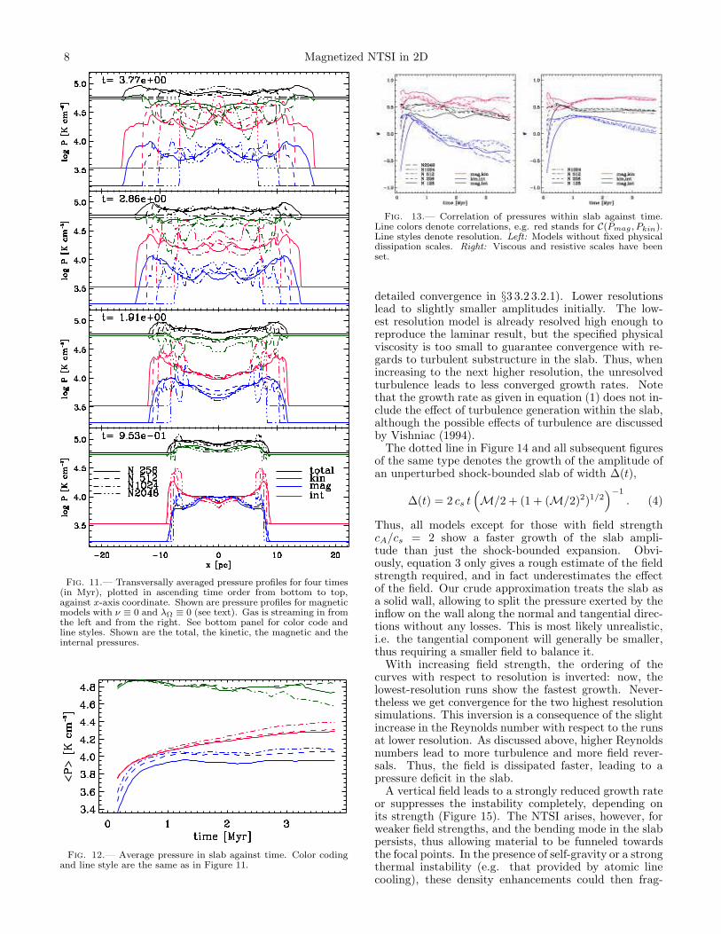
uation might be less extreme in a truly three-dimensionalsystem: a third field component without magnetic nullcould give rise to sufficient magnetic pressure to preventreconnection (see also Heitsch & Zweibel 2003). In thiscase, small-scale fields entangled by the turbulence in theslab could actually lead to additional pressure.The pressure profiles (Fig. 11) actually tell us a slightly

more complicated story than that of simple magnetic en-ergy dissipation. Pressures were averaged transversally(i.e. along the y-axis) and plotted against x, the in-flow direction. The magnetic pressure profile stays prettymuch at a constant level, independent of resolution andtime. What changes is the kinetic pressure, which dropsbelow its inflow value (all panels but bottom). This ef-fect gets stronger with increasing resolution. Thus, themagnetic field only acts as a dissipation channel for thekinetic energy. One could even interpret the kinetic pres-sure drop and simultaneous magnetic and internal (redlines) pressure rise as an attempt of the system to achieveequipartition (Fig. 12).This is not to say that the various pressure compo-

nents are in equilibrium, as the left panel of Figure 13

Fig. 10.— Logarithmic magnetic energy maps for models withviscosity ν ≡ 0 and resistivity λΩ = 0, i.e. the dissipation scaleis given by the grid resolution. Resolution increases from top tobottom (2562 to 20482 by factors of 2). Since the period in yis repeated four times, we show only one quarter of the domain.t = 3.8 Myr.

easily demonstrates. This panel shows the correlationcoefficient C for the three pairs of pressures, Pmag, Pint,and Pkin, for the case without (left) and with (right)a physical dissipation scale. Balance between the pres-sure components would show up as an anti-correlation,whereas a correlation can be interpreted as pressures be-ing in phase (and thus driving waves). Decorrelated pres-sures indicate a mixture. Kinetic and magnetic pressuredecorrelate at higher resolution, pointing to strong recon-nection events. Internal and magnetic pressure are onlyslightly correlated (see below), while kinetic and inter-nal pressure anti-correlate at late times, because high-density regions show more inertia. The models with afixed physical dissipation scale do not show strong reso-lution effects. Note, however, that the “dissipation-less”models are farther in the dynamical evolution than the“controlled” models, because of the different initial con-ditions (ky = 4 against ky = 1).These results demonstrate that only a fixed dissipa-

tive scale can guarantee full convergence of the modelswith resolution. Relying on numerical diffusion leads toflows with increasing Reynolds numbers as the resolu-tion increases and results that depend qualitatively andquantitatively on resolution.

3.3. Growth Rates

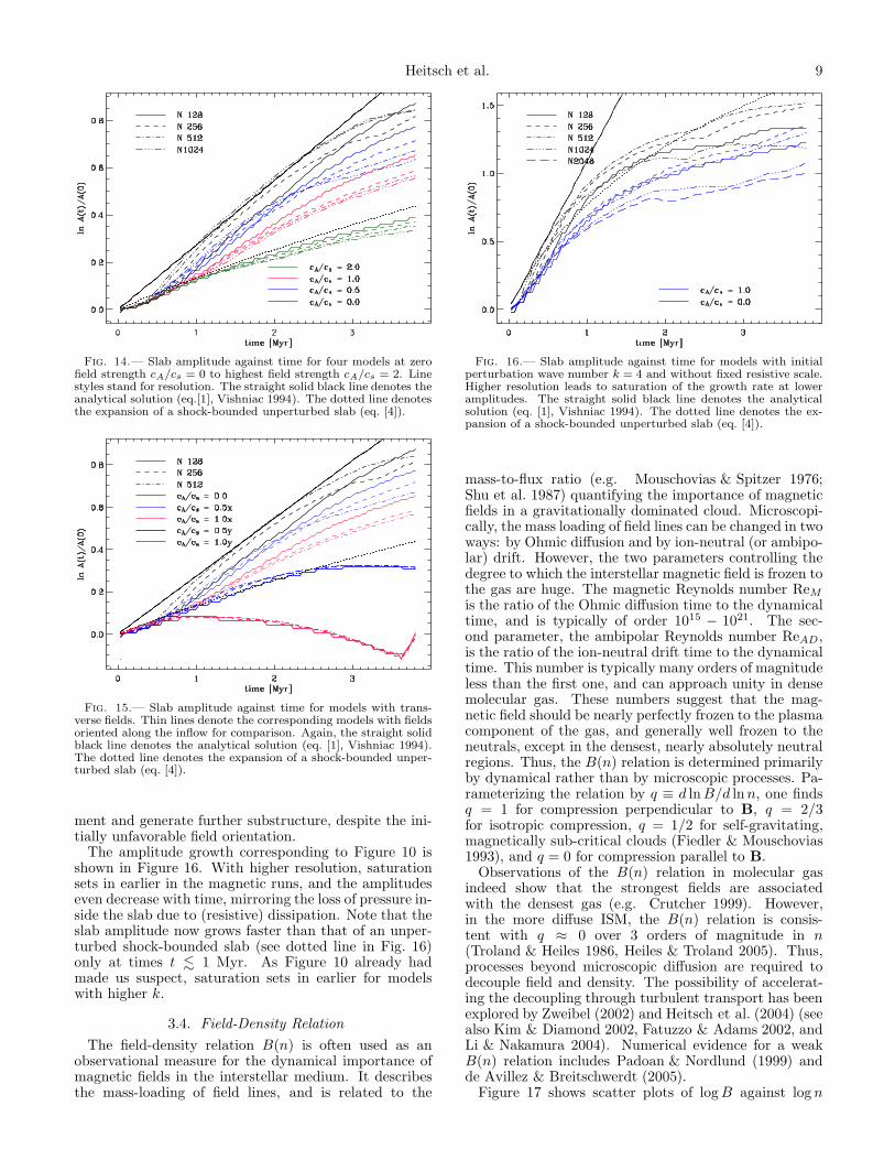
Figure 14 summarizes the growth of the slab’s ampli-tude with time. The hydrodynamical growth rates areconsistent with the analytical predictions (eq. [1], solidstraight black line). Saturation sets in when the focalpoints are shut off from the inflow (see also left col-umn of Fig. 6). The two highest resolution runs haveconverged also in terms of growth rates (we established

8 Magnetized NTSI in 2D

Fig. 11.— Transversally averaged pressure profiles for four times(in Myr), plotted in ascending time order from bottom to top,against x-axis coordinate. Shown are pressure profiles for magneticmodels with ν ≡ 0 and λΩ ≡ 0 (see text). Gas is streaming in fromthe left and from the right. See bottom panel for color code andline styles. Shown are the total, the kinetic, the magnetic and theinternal pressures.

Fig. 12.— Average pressure in slab against time. Color codingand line style are the same as in Figure 11.

Fig. 13.— Correlation of pressures within slab against time.Line colors denote correlations, e.g. red stands for C(Pmag , Pkin).Line styles denote resolution. Left: Models without fixed physicaldissipation scales. Right: Viscous and resistive scales have beenset.

detailed convergence in §3 3.2 3.2.1). Lower resolutionslead to slightly smaller amplitudes initially. The low-est resolution model is already resolved high enough toreproduce the laminar result, but the specified physicalviscosity is too small to guarantee convergence with re-gards to turbulent substructure in the slab. Thus, whenincreasing to the next higher resolution, the unresolvedturbulence leads to less converged growth rates. Notethat the growth rate as given in equation (1) does not in-clude the effect of turbulence generation within the slab,although the possible effects of turbulence are discussedby Vishniac (1994).The dotted line in Figure 14 and all subsequent figures

of the same type denotes the growth of the amplitude ofan unperturbed shock-bounded slab of width ∆(t),

∆(t) = 2 cs t(

M/2 + (1 + (M/2)2)1/2)

−1

. (4)

Thus, all models except for those with field strengthcA/cs = 2 show a faster growth of the slab ampli-tude than just the shock-bounded expansion. Obvi-ously, equation 3 only gives a rough estimate of the fieldstrength required, and in fact underestimates the effectof the field. Our crude approximation treats the slab asa solid wall, allowing to split the pressure exerted by theinflow on the wall along the normal and tangential direc-tions without any losses. This is most likely unrealistic,i.e. the tangential component will generally be smaller,thus requiring a smaller field to balance it.With increasing field strength, the ordering of the

curves with respect to resolution is inverted: now, thelowest-resolution runs show the fastest growth. Never-theless we get convergence for the two highest resolutionsimulations. This inversion is a consequence of the slightincrease in the Reynolds number with respect to the runsat lower resolution. As discussed above, higher Reynoldsnumbers lead to more turbulence and more field rever-sals. Thus, the field is dissipated faster, leading to apressure deficit in the slab.A vertical field leads to a strongly reduced growth rate

or suppresses the instability completely, depending onits strength (Figure 15). The NTSI arises, however, forweaker field strengths, and the bending mode in the slabpersists, thus allowing material to be funneled towardsthe focal points. In the presence of self-gravity or a strongthermal instability (e.g. that provided by atomic linecooling), these density enhancements could then frag-

Heitsch et al. 9

Fig. 14.— Slab amplitude against time for four models at zerofield strength cA/cs = 0 to highest field strength cA/cs = 2. Linestyles stand for resolution. The straight solid black line denotes theanalytical solution (eq.[1], Vishniac 1994). The dotted line denotesthe expansion of a shock-bounded unperturbed slab (eq. [4]).

Fig. 15.— Slab amplitude against time for models with trans-verse fields. Thin lines denote the corresponding models with fieldsoriented along the inflow for comparison. Again, the straight solidblack line denotes the analytical solution (eq. [1], Vishniac 1994).The dotted line denotes the expansion of a shock-bounded unper-turbed slab (eq. [4]).

ment and generate further substructure, despite the ini-tially unfavorable field orientation.The amplitude growth corresponding to Figure 10 is

shown in Figure 16. With higher resolution, saturationsets in earlier in the magnetic runs, and the amplitudeseven decrease with time, mirroring the loss of pressure in-side the slab due to (resistive) dissipation. Note that theslab amplitude now grows faster than that of an unper-turbed shock-bounded slab (see dotted line in Fig. 16)only at times t . 1 Myr. As Figure 10 already hadmade us suspect, saturation sets in earlier for modelswith higher k.

3.4. Field-Density Relation

The field-density relation B(n) is often used as anobservational measure for the dynamical importance ofmagnetic fields in the interstellar medium. It describesthe mass-loading of field lines, and is related to the

Fig. 16.— Slab amplitude against time for models with initialperturbation wave number k = 4 and without fixed resistive scale.Higher resolution leads to saturation of the growth rate at loweramplitudes. The straight solid black line denotes the analyticalsolution (eq. [1], Vishniac 1994). The dotted line denotes the ex-pansion of a shock-bounded unperturbed slab (eq. [4]).

mass-to-flux ratio (e.g. Mouschovias & Spitzer 1976;Shu et al. 1987) quantifying the importance of magneticfields in a gravitationally dominated cloud. Microscopi-cally, the mass loading of field lines can be changed in twoways: by Ohmic diffusion and by ion-neutral (or ambipo-lar) drift. However, the two parameters controlling thedegree to which the interstellar magnetic field is frozen tothe gas are huge. The magnetic Reynolds number ReMis the ratio of the Ohmic diffusion time to the dynamicaltime, and is typically of order 1015 − 1021. The sec-ond parameter, the ambipolar Reynolds number ReAD,is the ratio of the ion-neutral drift time to the dynamicaltime. This number is typically many orders of magnitudeless than the first one, and can approach unity in densemolecular gas. These numbers suggest that the mag-netic field should be nearly perfectly frozen to the plasmacomponent of the gas, and generally well frozen to theneutrals, except in the densest, nearly absolutely neutralregions. Thus, the B(n) relation is determined primarilyby dynamical rather than by microscopic processes. Pa-rameterizing the relation by q ≡ d lnB/d lnn, one findsq = 1 for compression perpendicular to B, q = 2/3for isotropic compression, q = 1/2 for self-gravitating,magnetically sub-critical clouds (Fiedler & Mouschovias1993), and q = 0 for compression parallel to B.Observations of the B(n) relation in molecular gas

indeed show that the strongest fields are associatedwith the densest gas (e.g. Crutcher 1999). However,in the more diffuse ISM, the B(n) relation is consis-tent with q ≈ 0 over 3 orders of magnitude in n(Troland & Heiles 1986, Heiles & Troland 2005). Thus,processes beyond microscopic diffusion are required todecouple field and density. The possibility of accelerat-ing the decoupling through turbulent transport has beenexplored by Zweibel (2002) and Heitsch et al. (2004) (seealso Kim & Diamond 2002, Fatuzzo & Adams 2002, andLi & Nakamura 2004). Numerical evidence for a weakB(n) relation includes Padoan & Nordlund (1999) andde Avillez & Breitschwerdt (2005).Figure 17 shows scatter plots of logB against logn

10 Magnetized NTSI in 2D

for four models, each measured at t = 4 Myr. The toprow shows models with the field parallel to the inflow(denoted by cAx in the label), while the field is orientedtransversally, or perpendicularly to the inflow in the bot-tom row (denoted by cAy). Idealized scalings are indi-cated by the dashed lines.The most striking difference between the top and the

bottom row is that for the configuration where the fieldis parallel to the inflow, field and density seem to corre-late more strongly than for the configuration where thefield is perpendicular to the inflow. This might seem sur-prising at first. After all, one would expect the field tobe correlated least with density if the gas is compressedalong the field lines (top row), and to be correlated mostwith density when the gas is compressed perpendicularlyto the field lines (bottom row). However, looking back atFigures 7 and 9 on the one hand, and Figure 10 on theother, we realize that the models with fields parallel tothe inflow generally develop turbulence, leading to fieldline stretching. Thus, in the (denser) slab, the field gen-erally will be stronger. Why, then, is there close to nocorrelation observable in the bottom row of Figure 17?The answer is hidden in the way we set up the initial con-ditions. To avoid the generation of strong MHD waves,we kept the field uniform, despite the fact that the flowcollision interface is strongly perturbed (see top row ofFig. 6 for the initial conditions). Thus, when gas is de-flected at the flanks (point “0” in Figure 5), it is essen-tially free to move along the field lines, i.e. transversally,but is increasingly prevented from continuing its trip to-wards the slab, because the magnetic pressure is increas-ing (note that the bulk magnetic field strength is higherin the bottom row of Fig. 17). Thus, the density can takeon any values in the slab, while the field value is givenby the ram pressure. A weaker field (lower right panel vslower left panel of Figure 17) reduces this effect, allowingsome scatter in the field strength, and, indeed, checkingFigure 9 for this case, the slab actually shows substruc-ture and is allowed to bend. Note that there is a strictd lnB/d lnn = 1 scaling for the strong field model (lowerleft panel), which results from the initial compression ofthe field lines.While it is hard to generalize the results of our two-

dimensional models, they demonstrate that the B(n) re-lation is strongly influenced by the geometry of the fieldsand the gas flows. Even compression perpendicular tothe field lines can lead to a nearly complete decouplingof field and density – as long as the gas flow is given thechance to break the symmetry.In a sense, we expect the “geometrical” mechanism

decoupling the field from the density (lower row of Fig-ure 17) to compete with the turbulent transport of themagnetic field: both act on dynamical (flow) timescales.For fields oriented perpendicularly to the inflow, ourmodels do not develop any substantial turbulence (thismight also be due to a too small Reynolds number). Onthe other hand, the models with field parallel to the in-flow direction do generate some turbulence. For thesemodels, B and n decorrelate only at higher density val-ues, corresponding to small scales, while the lower den-sity regions show a reasonably well established correla-tion between B and n.

4. summary

The Non-linear Thin Shell Instability (NTSI, Vishniac1994) is expected to occur in expanding shells, shocks orcolliding gas streams. Previous studies have addressedthe evolution of the NTSI under hydrodynamical condi-tions, including gravity and cooling. We have presenteda numerical study of the NTSI including magnetic fields.We have established that our numerical method is wellsuited to tackle the problem. We have found that the ef-fects of magnetic fields on the NTSI can be summarizedas follows:(1) Fields principally tend to weaken or even suppress

the NTSI. We further distinguish between two cases: (i)fields aligned with the inflow resist the transverse mo-mentum transport – which is the main driving agent ofthe NTSI – via the magnetic tension force; (ii) fields per-pendicular to the inflow lead to a stiffer equation of state.If cA ≈ u, the NTSI is suppressed. However, even fortransverse fields, substructures can form within the slab,which can serve as fragmentation seeds in the presenceof thermal instabilities or self-gravity.(2) A fixed physical scale both for viscous and resistive

dissipation is necessary to reach numerical convergence.When relying on numerical dissipation at the resolutionscale, the Reynolds number will increase with resolution,leading to a more turbulent environment and thus toresults which qualitatively and quantitatively depend onresolution (Figs 7, 10 and 16).(3) At larger Reynolds numbers, turbulent reconnec-

tion plays a role in the turbulent dense slab generatedby the NTSI. Magnetic energy is therefore dissipated athigher rates, leading to a pressure deficit in the denseslab. The magnetic field acts as a dissipation channel(Figs 11 and 12).(4) Although the energies (or average pressures) seem

to show a tendency of the system to evolve towardsequipartition, pressures do not balance locally withinthe slab (Figs. 12 and 13). Correlated pressures lead towaves, i.e. the slab’s inner structure is highly dynamical.(5) The relation between field and density is, at best,

weak in all models (Fig. 17). Models with fields paral-lel to the inflow exhibit a stronger B(n) correlation thanmodels with fields oriented perpendicularly to the inflow.The main reason for this is the generation of turbulence,which leads to field line stretching and thus field amplifi-cation within the denser slab. Fields oriented perpendic-ularly to the inflow allow instreaming material to movelaterally, permitting the field and density to decorrelate.Our isothermal models only allow a limited exploration

of the effect of fields on colliding flows in a thermally orgravitationally unstable medium. Clearly, substructurecan form in the slab under most conditions, providingpotential seeds for thermal or gravitational instabilities.Thus, to establish the role of magnetic fields for molec-ular cloud formation in the colliding flow scenario, thethermal and gravitational effects have to be addressed.

We thank E. Zweibel for a critical reading of themanuscript and for enlightening discussions, and E. Vish-niac for comments on magnetic field effects in theNTSI. Computations were performed at the NCSA(AST040026) and on the local resources at U of M, per-fectly administered and maintained by J. Hallum. Thiswork was supported by the University of Michigan and

Heitsch et al. 11

Fig. 17.— Scatter plots of magnetic field strength logB against density logn for models with parameters indicated in panels. Dashedlines denote idealized B(n)-scalings.

has made use of the NASA Astrophysics Data System.

REFERENCES

Balsara, D. S. 1998, ApJS, 116, 133Bergin, E. A., Hartmann, L. W., Raymond, J. C., & Ballesteros-

Paredes, J. 2004, ApJ, 612, 921Bhatnagar, P. L., Gross, E. P., & Krook, M. 1954, Physical Review,

94, 511Blondin, J. M. & Marks, B. S. 1996, New Astronomy, 1, 235Boldyrev, S., Nordlund, A., & Padoan, P. 2002, Physical Review

Letters, 89, 031102Cho, J. & Lazarian, A. 2003, MNRAS, 345, 325Crutcher, R. M. 1999, ApJ, 520, 706de Avillez, M. A. & Breitschwerdt, D. 2005, A&A, 436, 585Elmegreen, B. G. & Scalo, J. 2004, ARA&A, 42, 211Falgarone, E., Lis, D. C., Phillips, T. G., Pouquet, A., Porter, D. H.,

& Woodward, P. R. 1994, ApJ, 436, 728Fatuzzo, M. & Adams, F. C. 2002, ApJ, 570, 210Fiedler, R. A. & Mouschovias, T. C. 1993, ApJ, 415, 680Gardiner, T. A. & Stone, J. M. 2005, Journal of Computational

Physics, 205, 509Goldreich, P. & Sridhar, S. 1995, ApJ, 438, 763Hartmann, L., Ballesteros-Paredes, J., & Bergin, E. A. 2001, ApJ,

562, 852Hawley, J. F. & Stone, J. M. 1995, Comp. Phys. Comm., 89, 127Heiles, C. & Troland, T. H. 2005, ApJ, 624, 773Heitsch, F., Burkert, A., Hartmann, L. W., Slyz, A. D., &

Devriendt, J. E. G. 2005, ApJ, 633, L113Heitsch, F., Slyz, A. D., Devriendt, J. E. G., Hartmann, L. W., &

Burkert, A. 2006, ApJ, 648, 1052

Heitsch, F. & Zweibel, E. G. 2003, ApJ, 590, 291Heitsch, F., Zweibel, E. G., Slyz, A. D., & Devriendt, J. E. G. 2004,

ApJ, 603, 165Hueckstaedt, R. M. 2003, New Astronomy, 8, 295Kim, E.-j. & Diamond, P. H. 2002, ApJ, 578, L113Klein, R. I. & Woods, D. T. 1998, ApJ, 497, 777Li, Z.-Y. & Nakamura, F. 2004, ApJ, 609, L83Mouschovias, T. C. & Spitzer, Jr., L. 1976, ApJ, 210, 326Padoan, P. & Nordlund, A. 1999, ApJ, 526, 279Palotti, M. L., Heitsch, F., Zweibel, E. G., & Huang, Y.-M. 2006,

ApJ, submittedPassot, T., Vazquez-Semadeni, E., & Pouquet, A. 1995, ApJ, 455,

536Prendergast, K. H. & Xu, K. 1993, Journal of Computational

Physics, 109, 53Shu, C.-W. & Osher, S. 1988, J. Chem. Phys., 77, 439Shu, F. H., Adams, F. C., & Lizano, S. 1987, ARA&A, 25, 23Slyz, A., Devriendt, J. E. G., Bryan, G. L., Heitsch, F., & Silk, J.

2006, MNRAS, submittedSlyz, A. & Prendergast, K. H. 1999, A&AS, 139, 199Tang, H.-Z. & Xu, K. 2000, J. Chem. Phys., 165, 69Toth, G. & Odstrcil, D. 1996, J. Chem. Phys., 182, 82Troland, T. H. & Heiles, C. 1986, ApJ, 301, 339Vazquez-Semadeni, E., Passot, T., & Pouquet, A. 1995, ApJ, 441,

702Vazquez-Semadeni, E., Ryu, D., Passot, T., Gonzalez, R. F., &

Gazol, A. 2006, ApJ, 643, 245

12 Magnetized NTSI in 2D

Vishniac, E. T. 1994, ApJ, 428, 186Xu, K. 1999, J. Chem. Phys., 153, 334Zachary, A. L., Malagoli, A., & Collella, P. 1994,

J. Sci. Stat. Comput., 15, 263

Zweibel, E. G. 2002, ApJ, 567, 962