arX

iv:1

502.

0305

5v1

[as

tro-

ph.H

E]

10

Feb

2015

Draft version November 16, 2018Preprint typeset using LATEX style emulateapj v. 5/2/11

GAMMA-RAY BURST SPECTRA AND SPECTRAL CORRELATIONS FROM SUB-PHOTOSPHERICCOMPTONIZATION

Atul Chhotray and Davide LazzatiDepartment of Physics, Oregon State University, 301 Weniger Hall, Corvalis, OR 97331, USA

Draft version November 16, 2018

ABSTRACT

One of the most important unresolved issues in gamma-ray burst physics is the origin of the promptgamma-ray spectrum. Its general non-thermal character and the softness in the X-ray band remainunexplained. We tackle these issues by performing Monte Carlo simulations of radiation-matter in-teractions in a scattering dominated photon-lepton plasma. The plasma – initially in equilibrium – isdriven to non-equilibrium conditions by a sudden energy injection in the lepton population, mimickingthe effect of a shock wave or the dissipation of magnetic energy. Equilibrium restoration occurs dueto energy exchange between the photons and leptons. While the initial and final equilibrium spectraare thermal, the transitional photon spectra are characterized by non-thermal features such as power-law tails, high energy bumps, and multiple components. Such non-thermal features are observed atinfinity if the dissipation occurs at small to moderate optical depths, and the spectrum is releasedbefore thermalization is complete. We model the synthetic spectra with a Band function and showthat the resulting spectral parameters are similar to observations for a frequency range of 2-3 orders ofmagnitude around the peak. In addition, our model predicts correlations between the low-frequencyphoton index and the peak frequency as well as between the low- and high-frequency indices. Weexplore baryon and pair dominated fireballs and reach the conclusion that baryonic fireballs are abetter model for explaining the observed features of gamma-ray burst spectra.Subject headings: gamma-ray burst: general — radiation mechanisms: non-thermal

1. INTRODUCTION

The radiation mechanism that produces the bulk of theprompt emission of Gamma-Ray Bursts (GRBs) is stilla matter of open debate (e.g. Mastichiadis & Kazanas2009; Medvedev et al. 2009; Ryde & Pe’er 2009; Asanoet al. 2010; Ghisellini 2010; Lazzati & Begelman 2010;Daigne et al. 2011; Massaro & Grindlay 2011; Resmi& Zhang 2012; Hascoet et al. 2013; Crumley & Ku-mar 2013). Among the many proposed possibilities, thesynchrotron shock model (SSM) and the photosphericmodel (PhM) have recently gathered most of the atten-tion (Rees & Meszaros 1994; Piran 1999; Lloyd & Pet-rosian 2000; Meszaros & Rees 2000; Rees & Meszaros2005; Giannios 2006; Pe’er et al. 2006; Bosnjak et al.2009; Lazzati et al. 2009; Beloborodov 2010; Mizutaet al. 2011; Nagakura et al. 2011). Within the SSM,the bulk of the prompt radiation is produced by syn-chrotron from a non-thermal population of electrons gy-rating around a strong, locally-generated magnetic field.The non-thermal leptons are produced either by trans-relativistic internal shocks (the SSM proper, Rees &Meszaros 1994) or by magnetic reconnection in a Poynt-ing flux dominated outflow (e.g. the ICMART model,Zhang & Yan 2011). The SSM naturally accounts for thebroad, non-thermal nature of the spectrum. However, ithas difficulties in accounting for bursts with particularlysteep low-frequency slopes (Preece et al. 1998; Ghiselliniet al. 2000) and has limited predictive power, since theradiation properties are tied to poorly constrained quan-tities such as the lepton’s energy distribution, the ad-hoc equipartition parameters, and the ejection history ofshells from the central engine.The PhM does not specify a radiation mechanism, as-

suming instead that the burst radiation is produced inthe optically thick part of the outflow and advected out,its spectrum being the result of the strain between mech-anisms that tend to bring radiation and plasma in ther-mal equilibrium and mechanisms that can bring them outof balance (e.g., Beloborodov 2013). The PhM has beenshown to be able to reproduce ensemble properties of theGRB population, such as the debated Amati correlation,the Golenetskii correlation, and the recently discoveredcorrelation between the burst energetics and the Lorentzfactor of the outflow (Amati et al. 2002; Amati 2006;Liang et al. 2010; Fan et al. 2012; Ghirlanda et al.2012; Lazzati et al. 2013; Lopez-Camara et al. 2014).However, it is not yet understood how the broad-bandnature of the prompt spectrum, spanning many ordersof magnitude in frequency, is produced. In a hot, dissi-pationless flow, only the adiabatic cooling of the plasmawould work as a mechanism to break equilibrium, andthe GRB outflow would work as a miniature big bang,the entrained radiation maintaining a Planck spectrum.In a cold, dissipationless outflow, lepton scattering domi-nates the radiation-matter interaction producing a Wienspectrum (Rybicki & Lightman 1979). Outflows fromGRB progenitors are, however, far from dissipationless.Hydrodynamic outflows are continuously shocked out tolarge radii (Lazzati et al. 2009), and Poynting-dominatedoutflows suffer dissipation through magnetic reconnec-tion (Giannios & Spruit 2006). Either way, even if ther-mal equilibrium is reached at some point in the outflow,it is likely that such equilibrium is broken by a suddenrelease of energy in the lepton population or altered bya slow and continuous (or episodic) injection of energy.The effects of such energy injection on the photosphericspectrum are profound (e.g., Giannios 2006; Pe’er et al.

2

2006; Beloborodov 2010; Lazzati & Begelman 2010). Inaddition, the interaction between different parts of theoutflow in a stratified flow alter the thermal spectra into anon-thermal, highly polarized spectrum (Ito et al. 2013,2014; Lundman et al. 2013).In this paper we investigate the evolution of the radi-

ation spectrum following the sudden injection of energyin the lepton population of a plasma, assuming that theradiation and leptons interact via Compton scatteringand pair processes. We use a Monte Carlo (MC) methodthat evolves simultaneously the photon and lepton pop-ulations by performing inelastic scattering between pho-tons and leptons in both the non-relativistic and therelativistic (Klein-Nishina) regimes. The code also ac-counts for e−e+ annihilation (pair annihilation hence-forth) and e−e+ pair production from photon-photon col-lisions (pair production henceforth). We focus on tran-sient features that can be observed if the episode(s) ofenergy injection in the leptons occur at small or moder-ate optical depths (τ < 1000).This manuscript is organized as follows. In Section

2 we describe the physics and the methods of the MCcode, in Section 3 we show our results and in Section4 we discuss the results and compare them to previousfindings.

2. METHODOLOGY

2.1. Step 1: Particle Generation

As a first task, the code generates a user-defined num-ber of leptons and photons. Their energies follow a distri-bution that can be either of thermal equilibrium (Wienfor the photons and Maxwell-Juttner for the leptons) orany other user-specified distribution. After initializingthe photon and lepton distributions, our code performsthe following steps iteratively.

2.2. Step 2: Particle/Process selection

To initiate either a scattering or a pair event we needto select two particles1 - which we obtain by randomlyselecting a pair from our generated distributions. De-pending upon the particles selected, Compton scattering(if a photon and a lepton is chosen), pair annihilation (ifan e− or e+ is chosen) or pair production (if two photonsare chosen) is performed or another pair is re-selected ifany other combination occurs. After the selection, thecode proceeds with the following calculations:

1. Incident angle generation (θ) using the appropriaterelativistic scattering rates, under the assumptionthat both leptons and photons are isotropically dis-tributed.

2. Lorentz boost to the necessary reference frames(details explained in successive sections) from thelab frame.

3. Event probability computations from total crosssection (σ) calculations.

4. Scattering angle generation from differential crosssection ( dσ

dΩ).

1 Note that here particle can mean both a lepton or a photon.

5. Lorentz boost from the necessary frame back to thelab frame.

In the following sub-sections we discuss each of the threepossible processes in detail

2.2.1. Process 1: Compton Scattering

As the choice of reference frame is arbitrary, in the labframe we can assume that the lepton is traveling alongthe x-axis and the photon is incident upon the lepton inthe xy plane without any loss of generality. The angle ofincidence θγe between the chosen photon-lepton pair isgenerated by a probability distribution Pγe:

Pγe(βe, θγe) ∝ sin θγe(1− βe cos θγe) (1)

where βe = ve/c, is the ratio of lepton speed to the speedof light.To simulate the scattering event the code Lorentz trans-forms to the lepton frame (that we call the co-movingframe). The probability that the chosen photon-leptonpair interacts depends on the incident photon energy inthe co-moving frame. As Compton scattering becomesless efficient at higher energies, photons having energiescomparable to or greater than the lepton’s rest mass en-ergy are less likely to scatter. Using Monte Carlo sam-pling we determine if scattering occurs or not. This isdone by generating a random number and comparing itto the ratio of the Klein-Nishina cross section σγe to theThomson cross section, which we use as a reference value.We proceed with the scattering event if σγe/σT ≥ s1where s1 is a random number. If the condition is notsatisfied, the code returns to step 2. If instead the condi-tion is satisfied and the scattering occurs, the code gen-erates the polar scattering angle θ′s in accordance withthe Klein-Nishina differential cross-section formula

dσγe

dΩ=

r202

E′2s

E′2

(

E′

E′

s

+E′

s

E′− sin2 θ′s

)

(2)

where r0 is the classical radius of an electron, E′ andE′

s are the energies of the incident and scattered pho-ton respectively (e.g. Bluementhal & Gould 1970, Lon-gair 2003 and Rybicki & Lightman 1979). The energytransfer equation connecting E′ with E′

s is the Comptonequation (e.g. Bluementhal & Gould 1970, Longair 2003and Rybicki & Lightman 1979)

E′

s =E′

1 + E′

mec2(1 − cos θ′s)

. (3)

(Note here that θ′s is the angle that the scattered pho-ton makes with the direction of propagation of the inci-dent photon in the co-moving frame. Hence equations (2)and (3) hold true only in the lepton frame). Finally, theazimuthal angle φ′

s is generated randomly between zeroand 2π. Thus, we now have the four momenta of thescattered particles in the co-moving frame.

2.2.2. Process 2: Pair Production / Photon Annihilation

If the particle selection process selects two photonsthen the pair production/photon annihilation channel ischosen. The code computes the angle of incidence θγγbetween the chosen photons by using the probability dis-tribution Pγγ :

Pγγ(θγγ) ∝ sin θγγ(1− cos θγγ). (4)

3

To ensure that the photon pair has enough energy tolead to a pair production event the code checks the en-ergy of the photon/s in the zero momentum frame. Thezero momentum frame photon energy E′

o can be com-puted given the incident photon energies E1, E2 and theincident angle as

E′

o =√

E1E2 sin(θγγ/2). (5)

(Gould & Schereder 1967). If E′

o < mec2 the colliding

photon pair is not energetic energy to produce an e−e+

pair, hence the code jumps to step 2 for a new particlepair selection. Due to the energy dependence of cross-section σγγ , even photons exceeding the energy thresholdmight not produce pairs. To make this determination, weagain use the Thomson cross section as a reference anddetermine if the photon annihilation takes place by ran-domly drawing one number s2, obtaining σγγ by boost-ing to the center of momentum frame and evaluating ifσγγ/σT ≥ s2. If the inequality holds true, the code pro-ceeds with the pair production calculation. Otherwise,it is abandoned and the code returns to step 2.Once the photons succeed in producing leptons, the po-lar scattering angle θ′s of the newly born e− is computedfrom the pair annihilation differential cross section asgiven by

dσγγ

dΩ=

r20π

2b

(

mec2

E′

o

)2 1− b4 cos4 θ′s + 2(

mec2

E′

o

)2

b2 sin2 θ′s

(1− b2 cos2 θ′s)2 .

(6)(see Jauch & Rohrlich 1980, p.300) where b =√

1−(

mec2

E′

o

)2

. A random azimuthal angle φ′

s ∈ [0, 2π)

is assigned to the e−. Note that Lorentz transformationto the zero momentum frame is necessary because equa-tion (6) is frame dependent. Utilizing conservation laws,the four momenta of the e+ can be determined.

2.2.3. Process 3: Pair Annihilation/ Photon Production

The pair annihilation channel is chosen if the randomparticle selection constitutes an e−e+ pair. As with theother channels, we first determine the incident angle θee(subscript ee stands for lepton pair annihilation) betweenthe pair by computing the probability distribution ofscattering as given by

Pee(βe− , βe+ , θee) ∝ sin θeefkin (7)

where fkin as obtained from (Coppi & Blandford 1990)is given by:

fkin =√

β2e−

+ β2e+

− β2e−

β2e+

sin2 θee − 2βe−βe+ cos θee.

(8)Here βe =

veci.e. the ratio of lepton speed to the speed of

light. The code transforms all quantities to the rest frameof the electron to calculate the the total cross section σee

as (Jauch & Rohrlich 1980, p.269):

σee =r20π

β′2

(

γ′ + 1γ′

+ 4)

ln (γ′ +√

γ′2 − 1)− β′(γ′ + 3)

γ′(γ′ + 1)

(9)

where β′ = v′e+/c, γ′ = 1√

1−β′2i.e. the e+ speed and

Lorentz factor respectively in the co-moving frame trav-eling with the e−. On comparing the σee/σT with a ran-dom number s3 the code evaluates the occurrence of theannihilation event. If the event fails, the code returns tostep 2 to re-select another pair of particles. Following asuccessful event, the polar scattering angle θ′s between ei-ther of the pair produced photons is generated from thedifferential cross section (from Jauch & Rohrlich 1980,p.268)

dσee

dΩ=

r20π

β′γ′d

[

γ′ + 3−[1 + d]

2

(1 + γ′)d−

2(1 + γ′)d

[1 + d]2

]

(10)

where x = cos θ′s and d = γ′(1 − β′x). As pointed outin the preceding sub-sections, Lorentz transformation tothe electron frame is necessary as equation (10) is ex-pressed in terms of quantities defined in the electron’s co-moving frame. The random azimuthal angle φ′

s ∈ [0, 2π)is randomly assigned to either photon. Using conserva-tion laws, the four momenta of the pair produced photonscan be obtained.

2.3. Step 3: Back to the lab frame

At the end of the event, the code transforms the fourmomenta of the particles back to the lab frame by em-ploying Lorentz transformations. The loop is repeateduntil equilibrium is restored i.e. when the particle num-bers saturate and distributions become thermal.

3. RESULTS

We employ the Monte Carlo code described above tostudy the evolution of the radiation spectrum in a closedbox containing leptons and photons. The simulations areinitialized with a Wien radiation spectrum at 106 K anda non-equilibrium lepton population, either because lep-tons and photons are at different temperature or becausethe leptons energy distribution is non-thermal. This isexpected to mimic a scenario in which the leptons andradiation were initially at equilibrium, but the leptonpopulation has been brought out of equilibrium by a sud-den energy release. Such energy release may be due toshocks in the fluid (e.g., Rees & Meszaros 1994; Laz-zati & Begelman 2010) or by magnetic reconnection in amagnetized outflow (e.g. Giannios & Spruit 2006, McK-inney & Uzdensky 2012). As it will be clear at the end, afundamental parameter that determines the interactionbetween the photons and leptons is the particle ratio,i.e., the ratio of photon and lepton number densities. Ina GRB outflow, such a ratio can be readily estimated.Let us call EK the kinetic energy of the outflow carried

by particles with non-zero rest mass and Eγ the energyin electromagnetic radiation. We have:

Eγ

EK

=Nγhνpk

(

Np +me

mpNlep

)

Γmpc2

≃ 10−5 nγ

np +nlep

1836

(

hνpk1MeV

)

Γ−12 (11)

By calling η = Eγ/(Eγ + EK) the radiative efficiencyof the outflow, and assuming that matter and radiation

4

are coupled in the optically thick region and occupy thesame volume, equation (11) can be inverted to yield:

nγ

nlep=

105 η1−η

(

1MeVhνpk

)

Γ2 nlep = np

50 η1−η

(

1MeVhνpk

)

Γ2 nlep ≫ np

(12)

where the top line is valid for a non-pair enriched fireballwhile the bottom line is for a pair-dominated fireball. Allvalues in between are allowed for a partially pair-enrichedfireball. Note also that we used the convention Γ2 =Γ/102. GRB fireballs are therefore photon-dominated,even if highly pair-enriched.We here consider two possible values of the parti-

cle ratio. As a representative of pair-enriched plasma,we explore the case nγ/nlep = 10. A non-enrichedplasma (or photon-rich plasma) is represented by the ra-tio nγ/nlep = 1000. Note that the latter value is notas extreme as the one in equation (12). It is, however,technically challenging to simulate any higher value ofthe particle ratio. To ensure that the statistics of thelepton population is under control, we need to simu-late at least 1000 irreducible electrons (electrons thatare not possibly annihilated by a positron). For a parti-cle ratio nγ/nlep = 105, that would require the simula-tion of 108 photons. We believe that the adopted valuenγ/nlep = 1000 does capture the characteristics of thespectrum emerging from a photon-rich plasma and wewill discuss the consequences of higher particle ratios inSection 4.For each particle ratio, we explore different scenarios

in which the accelerated leptons are either thermal (Laz-zati & Begelman 2010) or non-thermal (e.g. Giannios2006; Pe’er et al. 2006; Beloborodov 2010) and we con-sider the possibility of multiple acceleration events, inwhich the leptons are re-energized before the equilibriumis reached. Some of these possibilities have been previ-ously explored, in particular the Comptonization froma non-thermal population of electrons (e.g. Pe’er et al.2006). We do not consider in this study continuous en-ergy injection, in which a stationary equilibrium betweenphotons and electrons is reached, and for which our codeis not well suited (e.g. Giannios 2006; Pe’er et al. 2006).All simulations are run until equilibrium is attained.

Here we define equilibrium as the time at which the spec-tral shape does not change with further collisions andthe number of photons and leptons saturate. This isgenerally much later than the time at which the totalenergies in leptons and photons approach their asymp-totic values, since a very small amount of energy canmake a significant difference in the tails of the distribu-tion, which are the interesting aspect of the spectrum forthis study. Our simulations do not have a time stamp,since all processes involved are scale free. A time stampcan be added upon deciding on a particle and photondensity, rather than a total number as specified in thecode. A meaningful comparison with the data can beaccomplished by considering that a photon in a relativis-tic outflow with Thomson opacity τ scatters-off/collideswith leptons an average number of times nsc ≃ τ be-fore being detected by an observer at infinity (e.g. Pe’eret al. 2005). Here we adopt as the Thomson opacityof a medium τ =

∫

nlepσT ds (see Rybicki & Lightman1979). It is possible therefore to look at our spectra in

101

102

103

104

105

106

10-3 10-2 10-1 100 101 102 103101

102

103

104

105

106

Initial Spectra

τdiss = 0.001

τdiss = 0.05

τdiss = 5.0

τdiss = 75.0

τdiss = 2246.0

Energy (keV)

F(E

)

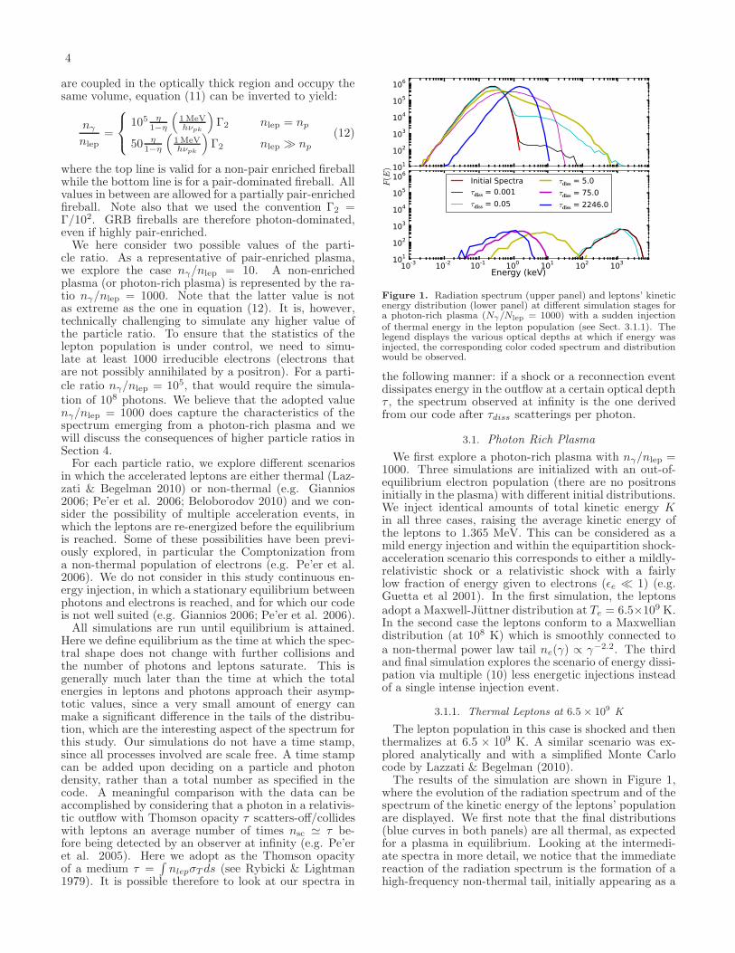
Figure 1. Radiation spectrum (upper panel) and leptons’ kineticenergy distribution (lower panel) at different simulation stages fora photon-rich plasma (Nγ/Nlep = 1000) with a sudden injectionof thermal energy in the lepton population (see Sect. 3.1.1). Thelegend displays the various optical depths at which if energy wasinjected, the corresponding color coded spectrum and distributionwould be observed.

the following manner: if a shock or a reconnection eventdissipates energy in the outflow at a certain optical depthτ , the spectrum observed at infinity is the one derivedfrom our code after τdiss scatterings per photon.

3.1. Photon Rich Plasma

We first explore a photon-rich plasma with nγ/nlep =1000. Three simulations are initialized with an out-of-equilibrium electron population (there are no positronsinitially in the plasma) with different initial distributions.We inject identical amounts of total kinetic energy Kin all three cases, raising the average kinetic energy ofthe leptons to 1.365 MeV. This can be considered as amild energy injection and within the equipartition shock-acceleration scenario this corresponds to either a mildly-relativistic shock or a relativistic shock with a fairlylow fraction of energy given to electrons (ǫe ≪ 1) (e.g.Guetta et al 2001). In the first simulation, the leptonsadopt a Maxwell-Juttner distribution at Te = 6.5×109 K.In the second case the leptons conform to a Maxwelliandistribution (at 108 K) which is smoothly connected toa non-thermal power law tail ne(γ) ∝ γ−2.2. The thirdand final simulation explores the scenario of energy dissi-pation via multiple (10) less energetic injections insteadof a single intense injection event.

3.1.1. Thermal Leptons at 6.5× 109 K

The lepton population in this case is shocked and thenthermalizes at 6.5 × 109 K. A similar scenario was ex-plored analytically and with a simplified Monte Carlocode by Lazzati & Begelman (2010).The results of the simulation are shown in Figure 1,

where the evolution of the radiation spectrum and of thespectrum of the kinetic energy of the leptons’ populationare displayed. We first note that the final distributions(blue curves in both panels) are all thermal, as expectedfor a plasma in equilibrium. Looking at the intermedi-ate spectra in more detail, we notice that the immediatereaction of the radiation spectrum is the formation of ahigh-frequency non-thermal tail, initially appearing as a

5

−8

−6

−4

−2

0

2α,β

α

β

0 100 200 300 400 500τdiss

0.0

0.5

1.0

1.5

2.0

Ep(keV

)

Ep

Figure 2. Evolution of the Band parameters α, β and, Ep ofspectra from the simulation shown in Figure 1. The x-axis indicatesthe optical depth of energy injection.

10-1 100 10110-1

100

101

102

103

104

105

106

107α=0.15 β=-2.25 Epeak=1.037 keV

Energy (keV)

N(ν

)

Figure 3. Fitting of the Band parameters α, β and Ep of spectrafrom the simulation shown in Figure 1 at τdiss = 103.

new component (for spectra at τdiss = 0.001) and sub-sequently forming a continuous tail stemming from thethermal photon population (τdiss = 5). At a subsequentstage, the low-frequency part of the radiation spectrum isalso modified, with the spectral peak migrating to higherfrequencies and causing a flattening of the low-frequencycomponent (τdiss = 75). The figure shows that the spec-trum takes a very large number of scatterings for equi-librium restoration, especially for frequencies lower thanthe peak. For energy dissipation at optical depths up to∼ 100 a high-frequency non-thermal tail is observed. Anon thermal low-frequency tail is instead observed evenfor a larger optical depth, up to a few thousand.In order to quantify our synthetic transient spectra and

compare them with observations, we fit them to an an-alytic model. We adopt the widely used Band function(Band et al. 1993) and fit it to the data over a fre-quency range of three orders of magnitude. Althoughthe GRB spectra are in most cases more complex thana Band function (e.g. Burgess et al. 2014, Guiriec etal. 2011, 2013) this still constitutes a zero-order testthat any model should pass. We begin by computingthe mean frequency from our data and select neighbor-ing frequencies within 1.5 orders of magnitude around

101

102

103

104

105

106

10-3 10-2 10-1 100 101 102 103 104101

102

103

104

105

106

Initial Spectra

τdiss = 0.01

τdiss = 0.5

τdiss = 50.0

τdiss = 400.0

τdiss = 2200.0

Energy (keV)

F(E

)

Figure 4. Color coded photon spectrum (upper panel) and lep-tons’ kinetic energy distribution (lower panel) at different stages forthe photon-rich simulation discussed in Section 3.1.2. The legenddisplays the various optical depths at which if energy was injected,the corresponding color coded spectrum and distribution would beobserved.

the mean. This data set is binned in frequency and abest-fit Band function is obtained by minimizing the χ2.Figure 2 shows the evolution of the spectral parame-

ters α, β and Ep for increasing optical depths. We againemphasize that this should not be considered as a timeevolution, since the number of scattering is set by theoptical depth at which the energy is released in the lep-tons. A sample fit of the spectrum at τdiss = 103 tothe Band function is shown in Figure 3. The figure rep-resents a typical case, and shows that the Band modelfits well the frequencies around the peak but deviationsare observed for the lowest and highest frequencies. Wewill address this issue further in the discussion. The leg-end at the top of the figure shows the Band parametersfor the fit. An interesting aspect of these simulations isthat the low-frequency photon index α and the peak fre-quency are strongly anti-correlated. This is due to thefact that it is necessary that the peak frequency shifts tohigher values for the low-frequency spectrum to changefrom its thermal equilibrium shape. We also note thatthe high-energy slope anticipates the low-energy one, thenon-thermal features building-up earlier and disappear-ing faster. We will discuss in more detail these correla-tions and their implications in Section 4.

3.1.2. Maxwellian leptons at 108 K with a power law tailp = 2.2

Most models of internal shocks predict the accelera-tion of non-thermal particles. Comptonization of seedthermal photons by non-thermal leptons has been widelystudied in different scenarios and under different assump-tions (e.g. Giannios 2006; Pe’er et al. 2005, 2006). Inthis scenario the shock generates a non-thermal leptondistribution characterized by

N(E)dE ∝ γ−pdγ (13)

where γ is the lepton Lorentz factor and p = 2.2. Theresults of the simulation are shown in Figure 4, where wepresent the evolving radiation spectrum and distributionof the kinetic energy of the leptons’ population. We no-tice that the equilibrium photon and lepton distributions(blue curves) are thermal, as expected at equilibrium.

6

−8

−6

−4

−2

0

2α,β

α

β

0 100 200 300 400 500τdiss

0.0

0.5

1.0

1.5

2.0

Ep(keV

)

Ep

Figure 5. Evolution of the Band parameters α, β and Ep ofspectra from the simulation shown in Figure 4. The x-axis indicatesthe optical depth of energy injection.

We also notice that the spectrum appears non-thermalfor a wide range of opacities. Initially a prominent high-energy power-law tail is developed, for a very small opac-ity (or τdiss ∼ 0.01). As the injection opacity increases,the power-law tail is truncated at progressively lower fre-quencies, the peak frequency shifts to higher values, anda non-thermal tail at low-frequencies develops. The high-frequency tail disappears for τdiss ∼ 400, but even largeropacities are required to turn the low-frequency tail backto the scattering-dominated equilibrium spectrum. Wefit the Band function to our synthetic spectra and ob-tain Figure 5, which shows the evolution of the spectralparameters α, β and Ep for increasing injection opticaldepths. We also notice correlations between the spec-tral parameters α and the peak frequency, as discussedin Section 3.1.1.

3.1.3. Discrete Multiple Energy Injections

The presence of multiple minor shocks has been em-phasized in 2D axisymmetric numerical simulations ofjets in collapsars (e.g. Lazzati et al. 2009) and seemto be an even more common feature in 3D simulations(Lopez-Camara et al. 2013). Hence, to provide a morerealistic scenario for the energy injection we explore lep-ton heating by multiple energy injections mimicking mul-tiple shocks instead of a single more powerful one. Thetotal energy injected into the lepton population is identi-cal to the amount injected in the simulations discussed inSections 3.1.1 and 3.1.2. However, the energy is dividedinto 10 equal and discrete partitions with each one beinginjected and distributed uniformly among the leptons,after every million scatterings.The results of the MC simulation are shown in Fig-

ure 6, where the evolving radiation spectrum and thespectrum of the kinetic energy of the leptons’ populationare displayed. In comparison to Figures 1 and 4, twodifferences are apparent for small optical depths. First,the high-frequency tail develops much more slowly. Sec-ondly, the slowly developing tail does not extend to thesame high energies and in fact, it never approaches theMeV mark. Neither of these differences is surprising,given that a smaller amount of energy is injected at reg-ular intervals. The results of the Band function fittingare reported in Figure 7 and bring to our attention that

101

102

103

104

105

106

10-3 10-2 10-1 100 101 102101

102

103

104

105

106

Initial Spectra

τdiss = 1.01

τdiss = 3.08

τdiss = 9.1

τdiss = 50.0

τdiss = 2300.0

Energy (keV)

F(E

)

Figure 6. Photon spectrum (upper panel) and leptons’ kinetic en-ergy distribution (lower panel) at different stages of the simulationdiscussed in Section 3.1.3. The legend associates the various opti-cal depths of energy injection with the corresponding color codedspectrum and distribution observed.

−8

−6

−4

−2

0

2

α,β

α

β

0 100 200 300 400 500τdiss

0.0

0.5

1.0

1.5

2.0

Ep(keV

)

Ep

Figure 7. Evolution of the Band parameters α, β and Ep ofspectra from the simulation shown in Figure 6. The x-axis displaysthe opacity at which energy deposition occurred.

−5

−4

−3

−2

−1

0

1

2

α,β

α

β

0 2 4 6 8 10 12τdiss

0.0

0.1

0.2

0.3

0.4

0.5

Ep(keV

)

Ep

Figure 8. Magnified version of Figure 7 depicting the response ofthe Band function parameters α, β and Ep to discrete and multipleenergy injections, indicated by the broken black vertical lines. Thex-axis displays the opacity at which energy deposition occurred.

7

like previous other simulations, the high-frequency pho-ton index β is the first to respond, and also the first todrop just when the α parameter reaches it’s minimumvalue. Another remarkable aspect of the multiple injec-tion scenario is the immediate reaction of the spectrumto new injections, especially for the high-frequency pho-ton index and the peak frequency (see Figure 8).What is perhaps mostly interesting, rather than the sub-tle differences among the three scenarios discussed here,is the fact the Band parameters of Figures 2, 5, and 7show remarkably similar behavior, even though the injec-tion scenarios are very different. In all three cases, injec-tion at low optical depth only produces a high-frequencypower-law tail. Injection at moderate optical depths(τdiss ∼ 10 − 100) produces a high-frequency power-lawtail, a shift in the peak frequency, and a non-thermallow-frequency tail. Injection at high to very high opticaldepths only results in a non-thermal low-frequency tail(see also Section 4 for a discussion).

3.2. Pair Enriched Plasmas

In this section we investigate plasmas enriched bye−e+ pairs, by choosing nγ/nlep = 10. GRB plasmascan become pair enriched via energy injection throughshocks/magnetic dissipation (Rees & Meszaros 2005;Meszaros et al. 2002; Pe’er & Waxman 2004) and if thepeak energy of the resulting distribution exceeds 20 keV(Svensson 1982). The generation of pairs is also evidentfrom the photon and lepton distributions crossing the 511keV mark as shown in the simulations in Sections 3.1.1and 3.1.2. We assume, as in the previous scenario, thatthe the pair enriched leptons are impulsively heated byinjecting equal amounts of kinetic energy K/10 for thefirst two simulations, albeit with different distributionfunctions (Maxwellian and Maxwellian plus power law).The third simulation explores the spectral evolution of apair enriched plasma with an even greater kinetic energyinjection. The initial photon count of the plasma Nγ is1.01 × 105. Being pair-enriched, the total lepton countNe of the plasma is 1.01× 104,

Ne = Ne− + 2Ne+e− = 102 + 104 (14)

where Ne− are electrons associated with protons andNe+e− denotes the number of pairs in the system.

3.2.1. Maxwellian leptons

We initiate the simulation with Maxwellian pair-enriched leptons that have been impulsively heated to108 K, thereby taking the population out of equilibriumwith the photons. The results of the simulation are dis-played in Figure 9 with the upper panel depicting thephoton spectra and the lower panel illustrating the ki-netic energies of the leptons. Firstly, as observed in thesection on photon rich plasmas, the final (blue curve)spectra is consistent with the equilibrium Wien distri-bution. For τdiss ∼ 1 a bump is observed to spike nearthe annihilation line along with a power law tail (blackcurve). The lepton distribution also displays a two com-ponent distribution (black curve in the lower panel). Forτdiss ∼ 2.3, the power law tail extends farther to high fre-quencies and merges with the annihilation bump (cyancurve). On increasing the injection opacity to around 13,the low frequency spectrum flattens, the peak frequency

101

102

103

104

105

10-2 10-1 100 101 102 103101

102

103

104

105

106Initial Spectra

τdiss = 0.956

τdiss = 2.337

τdiss = 12.659

τdiss = 31.531

τdiss = 117.116

Energy (keV)

F(E

)

Figure 9. Photon spectrum (upper panel) and leptons’ kineticenergy distribution (lower panel) at different stages of the pair-enriched simulation discussed in Section 3.2.1. The legend displaysthe various optical depths at which if energy was injected, thecorresponding color coded spectrum and distribution would be ob-served.

−8

−6

−4

−2

0

2

α,β

α

β

0 10 20 30 40 50τdiss

0

20

40

60

80

100

120

140

Ep(keV

)

Ep

Figure 10. Evolution of the Band parameters α, β and Ep ofspectra from the simulation shown in Figure 9 for increasing valuesof energy-injection optical depths.

increases and the annihilation bump merges completelywith the initial Wien distribution (or the remnant ofthe initial spectrum) creating a non-thermal flattenedplateau-like feature (yellow curve). The high-frequencypower law tail returns to the equilibrium Wien spectrummuch earlier (τdiss ≤ 32) than the non-thermal low fre-quency tail, which requires about (τdiss ∼ 100) to formthe equilibrium spectrum. We interpret this behavior tothe inability of the plasma to support a large populationof pairs. As a consequence the pairs quickly annihilateand a large amount of ∼ 511 keV photons are injected inthe plasma.The Band parameters obtained by fitting the Band func-tions to the simulation spectra are plotted in Figure 10.We note that for moderate optical depths, α = −0.75and β = −1.15 which corresponds to an extremely non-thermal spectrum. We also observe from the lower panelof Figure 10 that Ep = 20−40 keV. Furthermore, an anti-correlation is observed between the Band parameters αand β and between α and Ep.

8

101

102

103

104

105

10-2 10-1 100 101 102 103101

102

103

104

105

106

107Initial Spectra

τdiss = 0.098

τdiss = 1.879

τdiss = 12.656

τdiss = 45.045

τdiss = 130.631

Energy (keV)

F(E

)

Figure 11. Photon spectrum (upper panel) and leptons’ kineticenergy distribution (lower panel) at different stages of the simu-lation discussed in Section 3.2.2. The legend associates the vari-ous optical depths of energy injection with the corresponding colorcoded spectrum and distribution observed.

−8

−6

−4

−2

0

2

α,β

α

β

0 10 20 30 40 50τdiss

0

20

40

60

80

100

120

140

Ep(keV

)

Ep

Figure 12. Evolution of the Band parameters α, β and Ep ofspectra from the simulation shown in Figure 11. The x-axis dis-plays the opacity at which energy injection occurred.

3.2.2. Maxwellian leptons at 108 K with a power law tail

This simulation initializes the lower energy lepton pop-ulation as thermally distributed at 108 K and a higherenergy population with a power law tail. However, pairenrichment and constraining the injected kinetic energyto K/10 lowers the average kinetic energy per lepton incomparison to the photon-rich plasmas. As a result theleptons are generated according to the distribution

N(E)dE ∝ (γ − 1)−pd(γ − 1) (15)

where γ is the lepton’s Lorentz factor and p = 2.2. Thered curve in lower panel of Figure 11 displays the ini-tial kinetic energy distribution of the lepton population.Note that the power law tail does not extend to high ener-gies as the tail in Figure 4 does. The figure also shows theevolution of the photon spectra and leptons’ kinetic en-ergy as equilibrium restoration occurs. For the photons,the initial spectra (red curve) and equilibrium spectrum(blue curve) fit the Wien distribution. As is expected,pair annihilation produces a hump in the vicinity of the511 keV region. Meanwhile, the photons forming the ini-

101

102

103

104

105

10-2 10-1 100 101 102 103 104101

102

103

104

105

106Initial Spectra

τdiss = 0.049

τdiss = 0.98

τdiss = 3.405

τdiss = 13.902

τdiss = 72.273

Energy (keV)

F(E

)

Figure 13. Photon spectrum (upper panel) and leptons’ kineticenergy distribution (lower panel) at different stages of the pair-enriched simulation discussed in Section 3.2.3. The legend asso-ciates the various optical depths of energy injection with the cor-responding color coded particle spectrum and distribution.

tial Wien spectrum form a power law tail. Similar to theprevious scenario, at around τdiss ∼ 2 , the power lawextends to high frequencies and merges with the grow-ing annihilation hump (cyan curve). We also observea two component distribution in the lepton panel. Byτdiss ∼ 13, the two component spectrum transforms intoa broad band flat-plateau like spectrum (yellow curve)with the low-frequency spectrum being modified as well.The high frequency spectrum of the magenta curve (forτdiss ∼ 45) assumes the exponential cut-off of the Wienspectrum while the low-frequency tail is still prominent.These features make the transient spectra highly non-thermal.A comparison of Figure 9 with Figure 11 informs us thatthe spectra of these two scenarios are quite similar. Con-sequently, a comparison among Figure 10 and Figure 12also exhibits very similar results - including the anti-correlations between α and peak frequency and betweenα and β.

3.2.3. Maxwellian leptons at 108 K with a power law tailp = 2.2

This section explores the system when pair en-riched leptons are distributed according the Maxwell-Boltzmann distribution at 108 K for lower energieswhereas the high energy ones form a power-law tail withindex p = 2.2.Similar to the previously discussed cases, the photon

spectrum fits the Wien spectrum at equilibrium inFigure 13. A remarkable difference between Figure 13,and between Figures 9 and 11 is that the high frequencypower law tail catches up with the pair-annihilationmuch earlier (τdiss << 0.05) as depicted by the blackcurve. Remnants of the hump are visible in the blackand cyan curves. Furthermore, for less than 1 scat-terings, the low frequency tail becomes softer thanthe Wien spectrum (cyan curve). Another importantnon-thermal feature is the broadband nature of theflattened spectrum (the yellow curve extends over fourorders of magnitude in frequency). By about τdiss ∼ 14,the truncated high frequency tail approaches the expo-nential cut-off of the Wien spectrum, whereas the soft

9

−8

−6

−4

−2

0

2α,β

α

β

0 10 20 30 40 50τdiss

0

50

100

150

200

250

300

350

Ep(keV

)

Ep

Figure 14. Evolution of the Band parameters α, β and Ep ofspectra from the simulation shown in Figure 13 with increasingenergy-injection opacity.

10-2 10-1 100 101 1020.00

0.01

0.02

0.03

0.04

0.05

0.06

τdiss

Ne(10

5)

Ne−

Ne+

Ne− (Thermal)

Ne+ (Thermal)

Figure 15. Evolution of lepton count Ne for the simulations inSection 3.2.1 (labeled as Thermal) and 3.2.3. Note that the lep-ton count evolution of the simulations discussed in Sections 3.2.1and 3.2.2 is indistinguishable. The x-axis displays the opacity atwhich energy injection occurred.

low frequency tail still persists.The best-fit Band function obtained by χ2 minimizationtechnique, produces highly non-thermal spectral indices(α and β) but the peak frequency as shown in Figure 14is relatively high for GRBs. The lack of smoothnessin the α values for moderate optical depths is due tothe flatness of the photon spectrum as seen from theyellow curve in Figure 13, which occurs in conjunctionwith the transient saturation phase in the lepton count(see Figure 15). Figure 15 also displays and comparesthe lepton count for the simulation in Section 3.2.1 (thecurves labeled as Thermal, which are indistinguishablefrom the pair evolution in Section 3.2.2). Althoughthe initial lepton content of the plasmas in the threediscussed simulations is identical, the plasma with agreater kinetic energy injection can sustain pairs forlarger optical depths leading to a much broader andflatter spectrum. For moderate number of scatter-ings, we obtain α = −1 and β = −0.95. Again, ananti-correlation is found to exist between the param-eters α and β and also between α and the peak frequency.

−1.0 −0.5 0.0 0.5 1.0 1.5 2.0α

10-2

10-1

100

101

102

Ep(keV

)

Thermal

Thermal + Tail

Injection

Thermal

Thermal + Tail

Thermal + High Energy Tail

Figure 16. Plot of Band parameters Ep and α for the various sim-ulations discussed. The solid curves represent photon-rich plasmas

(Nγ

Nlep= 1000) whereas the broken curves are indicative of pair-

enriched plasmas where (Nγ

Nlep= 10). Note the similarity among

the curves and the exhibited anti-correlation.

−1.0 −0.5 0.0 0.5 1.0 1.5 2.0α

−4.0

−3.5

−3.0

−2.5

−2.0

−1.5

−1.0

−0.5

βThermal

Thermal + Tail

Injection

Thermal

Thermal + Tail

Thermal + High Energy Tail

Figure 17. Plot of Band parameters β and α for the various sim-ulations discussed. The solid curves represent photon-rich plasmas

(Nγ

Nlep= 1000) whereas the broken curves are indicative of pair-

enriched plasmas where (Nγ

Nlep= 10). Note the complex behavior

of the curves, especially the evolution of β.

4. SUMMARY AND DISCUSSION

We present Monte Carlo simulations of Compton scat-tering, e−e+ pair production, and e−e+ pair annihilationin GRB fireballs subject to mild to moderate internaldissipation. We explore cases of photon-rich media – asexpected in baryonic fireballs – and of pair-dominatedmedia. The leptonic component in our simulations isinitially set out of equilibrium by a sudden injection ofenergy and the spectrum is followed as continuous col-lisions among photons and leptons restore equilibrium.

We find that non-thermal spectra arise from transienteffects. Such spectra could be advected by the expandingfireball and released before equilibrium is reached if thedissipation takes place at optical depths of up to several

10

hundred. We show that the transient spectra can be rea-sonably fit by a Band function (Band et al. 1993) withina frequency range of 2-3 orders of magnitude around thepeak and could therefore explain GRB observations. Assuggested by Lazzati & Begelman (2010), non-thermalfeatures can arise even if both the photon and leptondistributions are initially thermal, provided that they areat different temperatures. As a matter of fact, we findthat the spectrum emerging from the fireball after a dis-sipation event at a certain optical depth does not dependstrongly on the way in which the energy was deposited inthe leptons. For the photon-rich cases, the first reactionof the photon spectrum to a sudden energy injection intothe leptons is the formation of a high-frequency power-law, either because non-thermal leptons are present orthrough the mechanism described in Lazzati & Begel-man (2010). If the injection happens at moderate opti-cal depths, the peak frequency of the photon spectrumalso shifts to higher frequencies and a non-thermal low-frequency tail appears. If the energy injection occurs atsomewhat large optical depths, the high frequency taildisappears and the spectrum presents a cutoff just abovethe peak. The low-frequency non-thermal tail is how-ever very resilient and only if the dissipation takes placeat very large optical depths, the equilibrium Wien spec-trum is attained. The pair-enriched simulations showa more complex behavior at low optical depths due topair processes, however we still observe the low frequencytail’s resilient behavior. We show that this phenomenol-ogy is rather independent on the details of the energydissipation process and generated lepton distributions:non-thermal leptons, high-temperature thermal leptons,and multiple discrete injection events all produce simi-lar spectra. For the case of the pair-enriched simulationshowever, we obtain peak frequencies that are somewhatlarge in the comoving frame (several hundred keV) mak-ing this scenario less interesting for explaining observedburst spectra. However their complex behavior and ex-treme peak energies offer a tantalizing explanation for therich diversity observed in peak energies of GRBs (Gold-stein et al 2012) especially when the peak energies >MeV.The conclusion we can glean from this study is there-

fore that comptonization of advected seed photons bysub-photospheric dissipation continues to be a viablemodel to explain the prompt gamma-ray bursts spec-trum. Agreement is particularly strong when the dis-sipation occurs at moderate optical depth (of the or-der of tens) so that both a high- and a low-frequencytail are produced. Dissipation at too low optical depthwould only produce a high-frequency tail, while dissipa-tion at too large optical depth would only produce a low-frequency tail. In a GRB dissipation is likely to occur atall optical depths (e.g. Lazzati et al. 2009). The dissipa-tion events that occur at moderate optical depth wouldtherefore be those mostly affecting the spectrum and giv-ing it its non-thermal appearance. Bursts characterizedby a Band spectrum over more than three orders of mag-nitude of frequency remain however challenging for thismodel, and other effects need to be invoked to avoid devi-ations from the pure power-law behavior at very low andhigh frequencies. Among these effects, some studied inthe literature are sub-photospheric, radiation mediatedmultiple shocks (Keren & Levinson 2014), line of sight

effects (Pe’er & Ryde 2011) and high-latitude emissions(Deng & Zhang 2014).

4.1. Spectral correlations

Besides finding that the overall shape of the partiallyComptonized spectra is qualitatively analogous to whatobserved in GRBs, we find that this model predicts theexistence of two correlations that can be used as a test ofits validity. We first notice an anti-correlation betweenthe low-energy photon index α and the peak frequency.The correlation is clearly seen in Figure 16, whereresults from all simulations are shown simultaneously.All simulations start with the same injected photonspectrum, the common point in the lower right of thediagram. The leptons in all three of the photon-richsimulations are energized to identical total kineticenergies K albeit different distribution functions. It isclear that the evolution of all photon-rich simulationsis virtually indistinguishable from each other. Asmore and more scatterings occur, the peak frequencyinitially grows and the low-frequency slope flattens.At moderate optical depths (∼ 100 in all three cases)the peak frequency reaches its maximum, the highfrequency tail disappears (shown in the Figure 17) andthe low-frequency tail begins to thermalize, dragging thepeak frequency to slightly lower values. The correlationhas two branches, a steeper one for τ < 100 and aflatter one at τ > 100. The second branch corresponds,however, to spectra without a high-frequency tail andis therefore not expected to represent observed GRBs.A similar pattern is followed by the pair-enriched cases,with the main difference that larger peak frequenciesare attained along with softer values for α and β. Theevolutionary curves for the pair-enriched cases showcomplexity due to the presence of pairs especially at lowopacities - with the simulation in Section 3.2.3 showinga greater amount of variability due to its ability tosustain pairs by temporarily balancing the number ofpair production and annihilation events (see Figure 15).In addition to the α − νpk anti-correlation, we alsofind hints of an anti-correlation between α and β.This correlation is shown in Figure 17 and is muchmore complex, reflecting the more complex behaviorof the high-frequency spectrum with respect to thelow-frequency one. In the case of the high-frequencyphoton-index β, the way in which the energy is injectedin the lepton population matters, each simulationproducing a different track on the graph.

Comparing these predictions to GRB spectral data isnot straightforward, since the correlations should not bestrong in observational data. Adding together data fromdifferent bursts, the correlations in the observer framewould be diluted by the different bulk Lorentz factors ofbursts and by the diversity of the particle ratio, radia-tion temperature, and dissipation intensity among bustsand pulses in a single burst. Still, some degree of cor-relation has been discussed in the literature, with con-tradictory conclusions as to its robustness. The α− νpkanti-correlation has been discussed in large burst samples(e.g. Amati et al. 2002; Goldstein at al. 2012; Burgesset al. 2014). The α-β anti-correlation has been observedfor some bursts (Zhang et al. 2011), however it is not acommon feature among GRBs.

11

Photospheric dissipation models have found it difficultto reproduce low frequency photon index α ∼ −1 andhave been unable to explain the GeV emissions (Zhanget al 2011). Figure 13 displays the emission spectra in therest frame of the burst and once Lorentz boosted the pho-tons forming the high frequency tail reach GeV energies.For low/moderate opacities, our simulations have consis-tently reproduced the low-energy photon index α < 0 asshown in Figure 16 thus providing a possible resolutionfor the mentioned issues. Our current model is unable toreproduce α < −1.1 for the parameter space explored,however additional effects such can modify and furthersoften the low frequency spectra. Analogous studies ofcomptonization effects in GRB outflows have been per-formed in the past, for example by Giannios (2006) andPe’er et al. (2006). Our work differs from both of theseprevious studies in both content and methodology. Gi-annios (2006) studied with Monte Carlo techniques theformation of the spectrum in magnetized outflows, con-sidering a particular form of dissipation and assumingthat the electrons distribution is always thermalized, al-beit at an evolving temperature. Pe’er et al. (2006),instead, used a code that solves the kinetic equationsfor particles and photons, and considered injection ofnon-thermal particles (as in our Section 3.1.2) as wellas continuous injection of energy in a thermal distribu-tion. None of these previous studies consider impulsiveinjection of energy in thermal leptons, as discussed hereor the case of multiple, discrete injection events. In an at-tempt to keep our results as general as possible we haveperformed the calculations in a static medium, ratherthan in an expanding jet. As long as the opacity atwhich the dissipation occurs is not too large, this shouldnot be a major limitation, and the advantage is thatour results are not limited to a particular prescriptionfor the jet radial evolution. In addition, most of the in-teresting results (the non-thermal spectra) are obtainedfor small and moderate values of the optical depth (or,analogously, of the number of scatterings that take placebefore the radiation is released). It should also be notedthat the assumption of an impulsive acceleration of theleptons that does not affect the photon spectra is likelynot adequate in a highly opaque medium. A final limi-tation of this study is that only moderate values of theparticle ratio can be explored. This is an inevitable lim-itation when both the lepton and photon distributionsare followed in the scattering process with a Monte Carlotechnique. If one of the two significantly outnumbers theother, a very large number of photons (or leptons) are re-quired, making the calculation extremely challenging andwould require parallelizing the code. While performingsuch simulations is important and will eventually becomepossible, we do not anticipate big phenomenological dif-ferences with respect to what we consider here. Evenwith less electrons, we expect the formation of a high-frequency tail (e.g. Lazzati & Begelman 2010), the subse-quent shift of the peak frequency accompanied by a flat-tening of the low-frequency photon index, and completethermalization only after many scatterings (i.e., only ifthe dissipation occurs at a very high optical depth).

ACKNOWLEDGMENTS

We thank the anonymous referee for her/his com-ments leading to improvement and clarity of the

manuscript. We thank Paolo Coppi for his adviceand insight into the physics of scattering and GabrieleGhisellini and Dimitrios Giannios for insightful discus-sions. This work was supported in part by NASAFermi GI grant NNX12AO74G and NASA Swift GI grantNNX13AO95G.

REFERENCES

Amati, L., Frontera, F., Tavani, M., et al. 2002, A&A, 390, 81Amati L. 2006, MNRAS, 372, 233Asano, K., Inoue, S., & Meszaros P. 2010, ApJ, 725, L121Band, D., Matteson, J., Ford, L., et al. 1993, ApJ, 413, 281Blumenthal, G.R., & Gould, R.J. 1970, Rev. Mod. Phys, 42, 237Beloborodov A. M. 2010, MNRAS, 407, 1033Beloborodov A. M. 2013, ApJ, 764, 157Bosnjak Z., Daigne F., & Dubus G. 2009, A&A, 498, 677Burgess, J. M., Ryde, F., & Yu, H.-F. 2014, arXiv:1410.7647Coppi P.S., & Blandford R.D. 1990, MNRAS, 245, 453Crumley P., & Kumar P. 2013, MNRAS, 429, 3238Daigne F., Bosnjak Z., & Dubus G. 2011, A&A, 526, A110Deng, W., & Zhang, B. 2014, ApJ, 785, 112Fan Y.-Z., Wei D.-M., Zhang F.-W., et al. 2012, ApJ, 755, L6Ghirlanda G., Nava L., Ghisellini G., et al. 2012, MNRAS, 420,

483Ghisellini G., Celotti A., & Lazzati D. 2000, MNRAS, 313, L1Ghisellini G. 2010, AIPC, 1248, 45fGiannios D. 2006, A&A, 457, 763Giannios D., & Spruit H. C. 2006, A&A, 450, 887Goldstein, A., Burgess, J.M., Preece, R.D., et al. 2012, ApJS,

199, 19Gould, R.J., & Schreder, G.P. 1967, Phy.Rev., 155, 1404Guetta, D., Spada, M., & Waxman, E. 2001, ApJ, 557, 399Guiriec, S., Connaughton, V., Briggs, M., et al. 2011, ApJ, 727, 33Guiriec, S., Daigne, F., Hascoet, R., et al. 2013, ApJ, 770, 32Hascoet R., Daigne F., & Mochkovitch R. 2013, A&A, 551, A124Ito,H., Nagataki, S., Ono, M., et al. 2013, ApJ, 777, 62Ito H., Nagataki S., Matsumoto J., et al. 2014, arXiv:1405.6284Jauch, J.M., & Rohrlich, F. 1980, Theory of Photons and

Electrons (2nd Extended ed.; New York: Springer-Verlag.)Keren, S., & Levinson, A. 2014, ApJ, 789, 128Lazzati D., Morsony B. J., & Begelman M. C. 2009, ApJ, 700, L47Lazzati D., & Begelman M. C. 2010, ApJ, 725, 1137Lazzati D., Morsony B. J., Margutti R., et al. 2013, ApJ, 765, 103Liang E.-W., Yi S.-X., Zhang J., et al. 2010, ApJ, 725, 2209Lloyd N. M., & Petrosian V. 2000, ApJ, 543, 722Longair, Malcolm, S. 2011, High Energy Astrophysics, (New

York: Cambridge)Lopez-Camara D., Morsony B. J., Begelman M. C., et al. 2013,

ApJ, 767, 19Lopez-Camara D., Morsony B. J. & Lazzati D. 2014, MNRAS,

442, 2202Lundman C., Pe’er A., & Ryde F. 2013, MNRAS, 428, 2430Massaro F., & Grindlay J. E. 2011, ApJ, 727, L1Mastichiadis A., & Kazanas D. 2009, ApJ, 694, L54McKinney J. C. & Uzdensky D. A. 2012, MNRAS, 419, 573Medvedev M. V., Pothapragada S. S. & Reynolds S. J. 2009,

ApJ, 702, L91Meszaros, P., Ramirez-Ruiz, E., Rees, M. J., et al. 2002, ApJ,

578, 812Meszaros P., & Rees M. J. 2000, ApJ, 530, 292Mizuta A., Nagataki S., & Aoi J. 2011, ApJ, 732, 26Nagakura H., Ito H., Kiuchi K., et al. 2011, ApJ, 731, 80Pe’er A., Meszaros P., & Rees M. J. 2005, ApJ, 635, 476Pe’er A., Meszaros P., & Rees M. J. 2006, ApJ, 642, 995Pe’er A., & Ryde, F., 2011, ApJ, 732, 49Pe’er, A., & Waxman, E. 2004, ApJ, 613, 448Piran T., 1999, PhR, 314, 575Preece R. D., Briggs M. S., Mallozzi R. S., et al. 1998, ApJ, 506,

L23Rees M. J., & Meszaros P. 1994, ApJ, 430, L93Rees M. J., & Meszaros P. 2005, ApJ, 628, 847Resmi L., & Zhang B. 2012, MNRAS, 426, 1385Rybicki, G.B. & Lightman, A.P. 1979, Radiative Processes in

Astrophysics, (New York: John Wiley)

12

Ryde, F., & Pe’er A. 2009, ApJ, 702, 1211Svensson, R. 1982, ApJ, 258, 335

Zhang, B., & Yan H. 2011, ApJ, 726, 90Zhang, B.B., Zhang, B., Liang, E.-W., et al. 2011, ApJ, 730, 141