ATK Nanowire Tutorial

Setup and Calculate the Properties of a Nanowire

Version 2015.2

ATK Nanowire Tutorial: Setup and Calculate the Properties of a Nano-

wire

Version 2015.2

Copyright © 2008–2015 QuantumWise A/S

Atomistix ToolKit Copyright Notice

All rights reserved.

This publication may be freely redistributed in its full, unmodified form. No part of this publication may be incorporated or used in other publications

without prior written permission from the publisher.

TABLE OF CONTENTS

1. Introduction ............................................................................................................ 1

2. Setting up the geometry ............................................................................................ 2

Nanowire custom builder ..................................................................................... 2

Hydrogen passivation of the structure .................................................................... 4

3. Relaxing the geometry of the nanowire ...................................................................... 8

Relaxing the nanowire using non-self-consistent tight binding ................................. 8

Relaxing the nanowire with DFT ........................................................................ 11

Bibliography ............................................................................................................. 15

iii

CHAPTER 1. INTRODUCTION

This tutorial focuses on the calculation and analysis of a silicon nanowire. You will learn how

to setup a nanowire with ATK, calculate the electronic and optical properties, and set up trans-

port calculations.

Some of the calculations in this tutorial are quite time-consuming; for a quicker introduction to

quantum transport studies with ATK, see the ATK Tutorial for Device Configurations.

It is assumed that you are familiar with the general workflow of VNL, as described in the basic

ATK Tutorial.

The DFT model in Atomistix ToolKit (ATK) is the underlying calculation engine used in this

tutorial. A complete description of all the parameters, and in many cases a longer discussion

about their physical relevance, can be found in the ATK reference manual.

1

CHAPTER 2. SETTING UP THE GEOMETRY

NANOWIRE CUSTOM BUILDER

To setup the nanowire geometry the nanowire builder in the Custom Builder will be used. Open

the tool by clicking the Custom Builder icon in the VNL toolbar.

Select Builders → Nanowire from the menu at the top of the tool. You should now see the

following.

The builder takes a cubic crystal structure and generates a nanowire using the Wulff construc-

tion. In this method you must specify the growth direction and the radius of the nanowire. The

shape of the nanowire is then determined by minimizing the surface energy, and for this purpose

you must specify the relative surface energy of the three main cubic surfaces, (100), (110) and

(111).

2

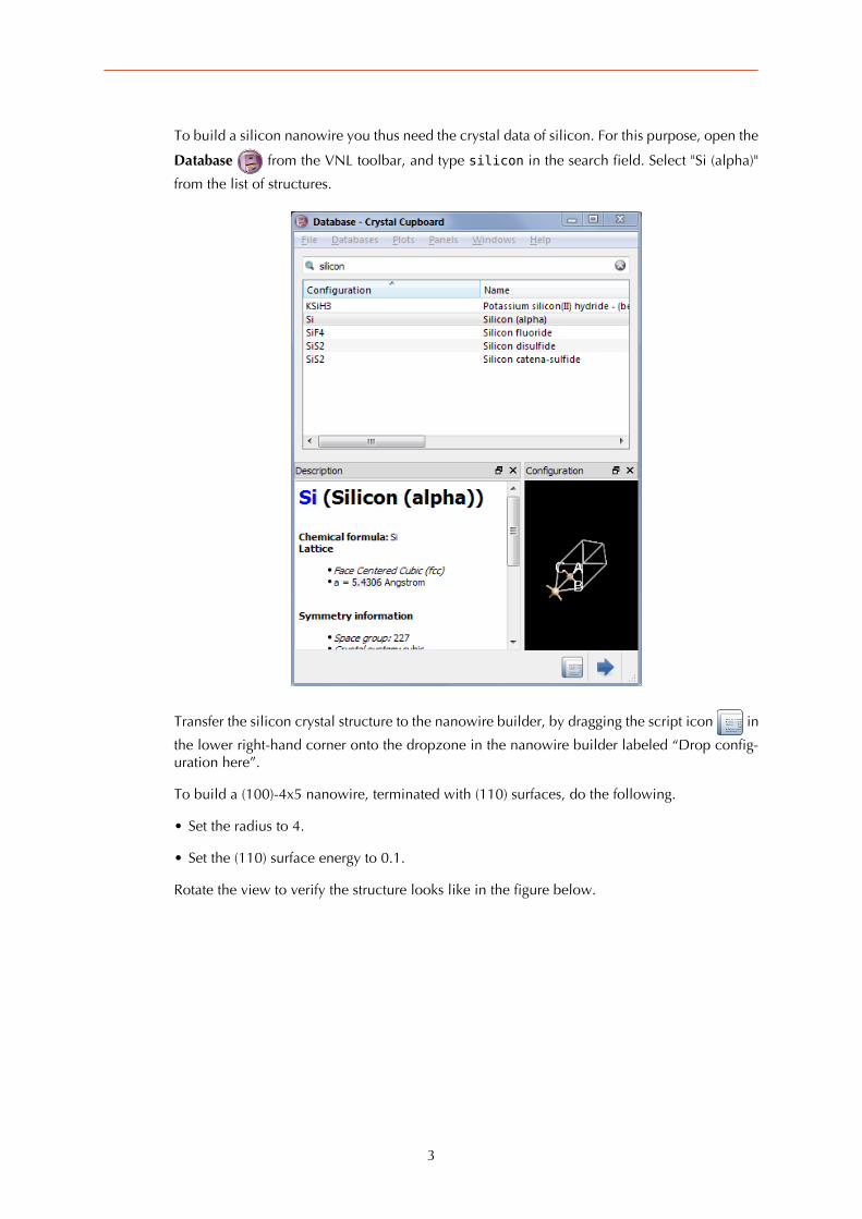
To build a silicon nanowire you thus need the crystal data of silicon. For this purpose, open the

Database from the VNL toolbar, and type silicon in the search field. Select "Si (alpha)"

from the list of structures.

Transfer the silicon crystal structure to the nanowire builder, by dragging the script icon in

the lower right-hand corner onto the dropzone in the nanowire builder labeled “Drop config-

uration here”.

To build a (100)-4x5 nanowire, terminated with (110) surfaces, do the following.

• Set the radius to 4.

• Set the (110) surface energy to 0.1.

Rotate the view to verify the structure looks like in the figure below.

3

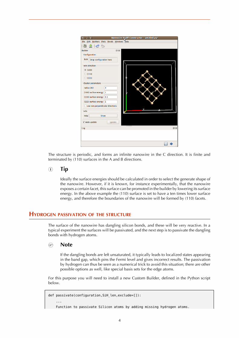
The structure is periodic, and forms an infinite nanowire in the C direction. It is finite and

terminated by (110) surfaces in the A and B directions.

Tip

Ideally the surface energies should be calculated in order to select the generate shape of

the nanowire. However, if it is known, for instance experimentally, that the nanowire

exposes a certain facet, this surface can be promoted in the builder by lowering its surface

energy. In the above example the (110) surface is set to have a ten times lower surface

energy, and therefore the boundaries of the nanowire will be formed by (110) facets.

HYDROGEN PASSIVATION OF THE STRUCTURE

The surface of the nanowire has dangling silicon bonds, and these will be very reactive. In a

typical experiment the surfaces will be passivated, and the next step is to passivate the dangling

bonds with hydrogen atoms.

Note

If the dangling bonds are left unsaturated, it typically leads to localized states appearing

in the band gap, which pins the Fermi level and gives incorrect results. The passivation

by hydrogen can thus be seen as a numerical trick to avoid this situation; there are other

possible options as well, like special basis sets for the edge atoms.

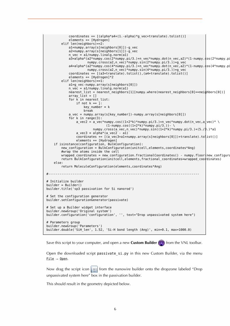
For this purpose you will need to install a new Custom Builder, defined in the Python script

below.

def passivate(configuration,SiH_len,exclude=[]):

''' Function to passivate Silicon atoms by adding missing hydrogen atoms.

4

Finds all atoms that dont have 4 nearest neighbors and attaches a hydrogen atom in such a way that all silicon atoms in a system have a sp3 structure.

Parameters: configuration : The configuration to be passivated SiH_len : The Si-H bond length exclude : A list of atoms (indices) not to be passivated

Returns: The passivated configuration '''

if configuration == None: return

nearest_neighbor_distance = 2.35152 alpha=SiH_len/nearest_neighbor_distance # Extract the original elements and coordinates (peel off units) # Extract the original elements and coordinates (peel off units) elements = numpy.array(configuration.elements()).tolist() num_atoms = len(elements) unitcell = configuration.bravaisLattice() c = configuration.cartesianCoordinates().inUnitsOf(Ang) coordinates = configuration.cartesianCoordinates().tolist()

if isinstance(configuration, BulkConfiguration): NA,NB,NC = (3,3,3) else: NA,NB,NC = (1,1,1)

supercell = configuration.repeat(NA,NB,NC) offset1 = NA*NB*NC/2 offset2 = offset1+1 s = supercell.cartesianCoordinates().inUnitsOf(Ang) super_coordinates = supercell.cartesianCoordinates().tolist() super_elements = configuration.elements()

# Compute the distance from each atom to all others (order N) distances = [] for i in s: distances.append(numpy.sqrt(((i-s)**2).sum(axis=1))) distances = numpy.array(distances)

# Determine which atoms are nearest neighbors, by the given criterion nearest_neighbors = numpy.where((distances<1.1*nearest_neighbor_distance) & \ (distances>1e-4))

# Count how many nearest neighbors each atoms has num_neighbors = [0,]*len(super_coordinates) for i in range(len(nearest_neighbors[0])): num_neighbors[nearest_neighbors[0][i]] += 1 # Filter out those atoms with only 2 nearest neighbors all_low_coordination_atoms = numpy.where((numpy.array(num_neighbors)<4))[0] in_original_cell = numpy.where((all_low_coordination_atoms>=num_atoms*offset1) & \ (all_low_coordination_atoms<num_atoms*offset2))[0] low_coordination_atoms = all_low_coordination_atoms[in_original_cell]

for j in low_coordination_atoms: i = j - num_atoms*offset1

# Exclude atoms that are in the "exclude" list if i in exclude or elements[i]!=Silicon: continue # Find neighbors of the low coordination atoms neighbors = nearest_neighbors[1][numpy.where(nearest_neighbors[0]==j)] g_vec = s[j] translate = s[i]-s[j] if len(neighbors)==3: a1=numpy.array(s[neighbors[0]]) a2=numpy.array(s[neighbors[1]]) a3=numpy.array(s[neighbors[2]]) a4=(4*g_vec-a1-a2-a3)

5

coordinates += [(alpha*a4+(1.-alpha)*g_vec+translate).tolist()] elements += [Hydrogen] elif len(neighbors)==2: a1=numpy.array(s[neighbors[0]])-g_vec a2=numpy.array(s[neighbors[1]])-g_vec n_vec = a1/numpy.linalg.norm(a1) a3=alpha*(a2*numpy.cos(2*numpy.pi/3.)+n_vec*numpy.dot(n_vec,a2)*(1-numpy.cos(2*numpy.pi/3.))- \ numpy.cross(a2,n_vec)*numpy.sin(2*numpy.pi/3.))+g_vec a4=alpha*(a2*numpy.cos(4*numpy.pi/3.)+n_vec*numpy.dot(n_vec,a2)*(1-numpy.cos(4*numpy.pi/3.))- \ numpy.cross(a2,n_vec)*numpy.sin(4*numpy.pi/3.))+g_vec coordinates += [(a3+translate).tolist(),(a4+translate).tolist()] elements += [Hydrogen]*2 elif len(neighbors)==1: a1=g_vec-numpy.array(s[neighbors[0]]) n_vec = a1/numpy.linalg.norm(a1) nearest_list = nearest_neighbors[1][numpy.where(nearest_neighbors[0]==neighbors[0])] array_list = [] for k in nearest_list: if not k == j: key_number = k break a_vec = numpy.array(s[key_number])-numpy.array(s[neighbors[0]]) for k in range(3): a_vec2 = a_vec*numpy.cos((1+2*k)*numpy.pi/3.)+n_vec*numpy.dot(n_vec,a_vec)* \ (1-numpy.cos((1+2*k)*numpy.pi/3.))- \ numpy.cross(a_vec,n_vec)*numpy.sin((1+2*k)*numpy.pi/3.)+(5./3.)*a1 a_vec3 = alpha*(a_vec2 - a1) coordinates += [(a_vec3+a1+numpy.array(s[neighbors[0]])+translate).tolist()] elements += [Hydrogen] if isinstance(configuration, BulkConfiguration): new_configuration = BulkConfiguration(unitcell,elements,coordinates*Ang) #wrap the atoms inside the cell wrapped_coordinates = new_configuration.fractionalCoordinates() - numpy.floor(new_configuration.fractionalCoordinates()) return BulkConfiguration(unitcell,elements,fractional_coordinates=wrapped_coordinates) else: return MoleculeConfiguration(elements,coordinates*Ang)

#---------------------------------------------------------------------------------

# Initialize builderbuilder = Builder()builder.title('sp3 passivation for Si nanorod')

# Set the configuration generatorbuilder.setConfigurationGenerator(passivate)

# Set up a Builder widget interfacebuilder.newGroup('Original system')builder.configuration('configuration', '', text="Drop unpassivated system here")

# Parameters groupbuilder.newGroup('Parameters')builder.double('SiH_len', 1.52, 'Si-H bond length (Ang)', min=0.1, max=1000.0)

Save this script to your computer, and open a new Custom Builder from the VNL toolbar.

Open the downloaded script passivate_si.py in this new Custom Builder, via the menu

File → Open.

Now drag the script icon from the nanowire builder onto the dropzone labeled “Drop

unpassivated system here” box in the passivation builder.

This should result in the geometry depicted below.

6

Note

The nanowire has only been passivated in the A/B plane. In the C-direction the structure

is periodic, and the half bonds on the outer-most atoms in this direction illustrate that

they have a bond to atoms in the neighbouring cell.

Save the geometry (File → Save) under the name si_nw45.py.

At this point the arrangement of the Si atoms corresponds to the bulk lattice constant of the

crystal. However, the atoms in the nanowire see a different environment than an infinite periodic

crystal, and so it can be expected that there will be some rearrangements of the positions, in

particular on the surface. Thus, your next task will be to relax the geometry of the structure.

7

CHAPTER 3. RELAXING THE GEOMETRY OF THE

NANOWIRE

RELAXING THE NANOWIRE USING NON-SELF-CONSISTENT TIGHT BINDING

You will now relax the geometry using a non-self-consistent tight-binding method. This is a very

fast method that gives reasonably accurate results for this system. Furthermore, it is a convenient

method to find out a good setting of the different accuracy parameters.

Select the geometry file created in the previous chapter, and drop it onto the Script Genera-

tor icon on the VNL toolbar.

•Add a New Calculator block.

•Add 2 OptimizeGeometry blocks.

•Add one more New Calculator block.

•Add an additional OptimizeGeometry block.

• Change the output filename to si_nw_tb.nc.

The Script Generator should now appears as in the figure below.

8

The idea is now to change the parameters for each relaxation, and check how sensitive the

results are to the parameters.

For the first calculator, setup a non-self-consistent tight-binding method with the following set-

tings.

• Select the ATK-SE: Slater-Koster calculator.

• Set the k-point sampling to (1,1,2).

• Under Slater-Koster basis set, make sure that DFTB (CP2K, non-self-consistent) is selected.

Note

The CP2K tight-binding parameters are generated by the CP2K consortium.

Next open the first OptimizeGeometry block

• Set the Maximum force to 0.02.

• Set the Maximum stress to 0.005.

• Remove the tick from the z-direction under Constrain cell.

9

The second OptimizeGeometry block will be used to check the effect of increasing the accuracy

of the optimization.

• Set the Maximum force to 0.01.

• Set the Maximum stress to 0.001.

• Again remove the tick from cell constraint in the z-direction.

The purpose of the last set of script blocks is to check if an increased k-point sampling will

modify the relaxed geometry.

Open the last New calculator block and make the following settings.

• Select the ATK-SE: Slater-Koster calculator.

• Set the k-point sampling to (1,1,8).

• Again, under Slater-Koster basis set, make sure that DFTB (CP2K, non-self-consistent) is se-

lected.

Repeat the settings of the first OptimizeGeometry block, i.e.

• Set the Maximum force to 0.01.

• Set the Maximum stress to 0.0005.

• Remove the constraint of the cell in the z-direction.

It is a good idea to save the script, for future reference.

10

EXECUTING AND ANALYSING THE RELAXATION

Now transfer the calculation to the Job Manager using the "Send to" button, and start the

calculation.

When the job finishes (it will only take a few minutes), save the log into a file si_nw_tb.log.

On inspection of the log file, several important observations can be made.

• The lowering of the total energy due to the increased threshold for the optimized geometry

is in the meV range.

• The error due to having as few as 2 k-points in the C-direction is negligible.

• The strain on the cell is very small, already in the intial configuration.

Thus, for the more expensive relaxations with the DFT model, you do not need to check the

accuracy of k-point sampling and force tolerance, but can stick to the choice used for the first

optimization. Moreover, it is not necessary to relax the strain.

RELAXING THE NANOWIRE WITH DFT

In the following you will relax the nanowire using a DFT model in order to check the accuracy

of the tight-binding model.

The GGA.PBE exchange-correlation functional in DFT is known to give accurate results for the

structure of geometries, also for semiconductors. To understand the accuracy of different basis

sets, as well as the tight-binding calculation, the first task is to compare the forces and stress

obtained with different basis sets.

CALCULATING DFT FORCES

In the VNL file browser locate the file si_nw45.py from before and drop it onto the Script

Generator icon in the VNL toolbar.

In the Script Generator, add a calculator and a Forces block from Analysis. Repeat this 3 times,

so in total you have 8 blocks.

Change the output file name to si_nw_gga_forces.nc.

11

The Next step is to modify the calculators. Open the first New Calculator block, and

• Select the ATK-SE: Slater-Koster calculator,

• set the k-point sampling to (1,1,2),

• and finally make sure that the DFTB (CP2K, non-self-consistent) basis set is selected.

Open the second calculator block and

• Select the ATK-DFT calculator,

• set the k-points to (1,1,2),

• select the GGA exchange correlation functional,

• and finally select the SingleZeta basis set for both Si and H.

Use the same DFT settings for the third calculator block, except

• change the basis set to DoubleZeta for both Si and H.

Finally, open the last calculator and again use the same DFT settings, exceot

• set the basis set to DoubleZetaPolarized (this is actually the default).

ANALYZING THE DFT FORCES

Transfer the script to the Job Manager and start the calculation.

The calculation will take 5-10 minutes. To analyze the forces, use the following small script.

#Read in list of forces objectsforces_objects = nlread('si_nw_gga_forces.nc', Forces)

#Comparing forces of the different basis setsn = len(forces_objects)norm_correlation = numpy.zeros(n*n).reshape(n,n)for i, forces1 in enumerate(forces_objects): f1 = forces1.evaluate().inUnitsOf(eV/Ang) for j, forces2 in enumerate(forces_objects): f2 = forces2.evaluate().inUnitsOf(eV/Ang) if i == j: norm_correlation[i,j] = numpy.linalg.norm(f1) else: norm_correlation[i,j] = numpy.linalg.norm(f1-f2)

12

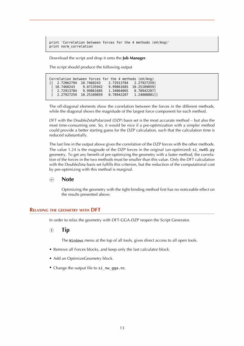
print 'Correlation between forces for the 4 methods (eV/Ang)'print norm_correlation

Download the script and drop it onto the Job Manager.

The script should produce the following output

Correlation between forces for the 4 methods (eV/Ang)[[ 2.72062794 10.7460243 2.72913784 2.27927259] [ 10.7460243 9.07135942 9.99861685 10.25109059] [ 2.72913784 9.99861685 1.34064065 0.78942207] [ 2.27927259 10.25109059 0.78942207 1.24008081]]

The off-diagonal elements show the correlation between the forces in the different methods,

while the diagonal shows the magnitude of the largest force component for each method.

DFT with the DoubleZetaPolarized (DZP) basis set is the most accurate method − but also the

most time-consuming one. So, it would be nice if a pre-optimization with a simpler method

could provide a better starting guess for the DZP calculation, such that the calculation time is

reduced substantially.

The last line in the output above gives the correlation of the DZP forces with the other methods.

The value 1.24 is the magnude of the DZP forces in the original (un-optimized) si_nw45.pygeometry. To get any benefit of pre-optimizing the geometry with a faster method, the correla-

tion of the forces in the two methods must be smaller than this value. Only the DFT calculation

with the DoubleZeta basis set fulfills this criterion, but the reduction of the computational cost

by pre-optimizing with this method is marginal.

Note

Optimizing the geometry with the tight-binding method first has no noticeable effect on

the results presented above.

RELAXING THE GEOMETRY WITH DFT

In order to relax the geometry with DFT-GGA-DZP reopen the Script Generator.

Tip

The Windows menu at the top of all tools, gives direct access to all open tools.

• Remove all Forces blocks, and keep only the last calculator block.

• Add an OptimizeGeometry block.

• Change the output file to si_nw_gga.nc.

13

Transfer the calculation to the Job Manager and start the calculation.

The job will take around an hour to finish.

Note

In relation to the discussion above about pre-optimization, it is interesting to note that

the relaxation goes through 17 optimization steps. If we start the relaxation from a ge-

ometry optimized with the tight-binding method, this number increases to 23. Thus,

indeed there is no gain in pre-optimizing this particular system. This is not to say this

approach is never useful; if the initial geometry is very far away from equillibrium, the

tight-binding method can be used to quickly get a better starting guess.

14

BIBLIOGRAPHY

[1] K. Stokbro, J. Taylor, M. Brandbyge, J.-L. Mozos, and P. Ordejón. Comp. Mat. Sci., 27, 151, 2003

[2] K. S. Thygesen, and K. W. Jacobsen. Chemical Physics, 319, 111-125, 2005

15