atmospheric acetylene and its relationship with co as an...

Atmospheric acetylene and its relationship with CO

as an indicator of air mass age

Yaping Xiao,1,2 Daniel J. Jacob,1 and Solene Turquety1,3

Received 20 November 2006; revised 12 February 2007; accepted 5 March 2007; published 21 June 2007.

[1] Acetylene (C2H2) and CO originating from combustion are strongly correlated inatmospheric observations, offering constraints on atmospheric dilution and chemicalaging. We examine here the C2H2-CO relationships in aircraft observations worldwide,and interpret them with simple models as well as with a global chemical transport model(GEOS-Chem). A C2H2 global source of 6.6 Tg yr�1 in GEOS-Chem simulates theensemble of global C2H2 observations without systematic bias, and captures most seasonaland regional features. C2H2/CO concentration ratios decrease from continental sourceregions to the remote atmosphere in a manner consistent between the observations and themodel. However, the dC2H2/dCO slope from the linear regression does not show such asystematic decrease, either in the model or in the observations, reflecting variability inbackground air. The slope b = dlog[C2H2]/dlog[CO] of the linear regression ofconcentrations in log space offers information for separating the influences of dilution andchemical aging. We find that a linear mixing model with constant dilution rate andbackground is successful in fresh continental outflow but not in remote air. A diffusionmodel provides a better conceptual framework for interpreting the observations, where thevalue of b relative to the square root of the ratio of C2H2 and CO chemical lifetimes(1.7–1.9) measures the relative importance of dilution and chemistry. We thus find thatdilution dominates in fresh outflow but chemical loss dominates in remote air. This resultis supported by GEOS-Chem sensitivity simulations with modified OH concentrations,and suggests that the model overestimates OH in the southern tropics.

Citation: Xiao, Y., D. J. Jacob, and S. Turquety (2007), Atmospheric acetylene and its relationship with CO as an indicator of air

mass age, J. Geophys. Res., 112, D12305, doi:10.1029/2006JD008268.

1. Introduction

[2] Acetylene (C2H2) and carbon monoxide (CO) havecommon sources from combustion and are highly correlatedin atmospheric observations [Blake et al., 1992, 1993, 1999,2001, 2003; Wofsy et al., 1992; Wang et al., 2003]. They areboth removed from the atmosphere by reaction with the OHradical, with mean lifetimes of about two weeks for C2H2

and 2 months for CO. A number of studies have used theobserved C2H2/CO concentration ratio as a tracer of the ageof air since it last encountered a combustion source region[Smyth et al., 1996; Gregory et al., 1997; Russo et al., 2003;Swanson et al., 2003], following the general use for thispurpose of hydrocarbon pairs with common sources anddifferent lifetimes [Parrish et al., 1992; McKeen and Liu,1993; Parrish et al., 2004; de Gouw et al., 2005]. TheC2H2-CO pair is of particular value for diagnosing the age

of air in the remote troposphere because the C2H2 lifetime islong and the observed correlation with CO remains strong.Beyond its qualitative use as a tracer of the age of air, theC2H2-CO relationship may offer important quantitativeinformation to test our understanding of OH levels andglobal atmospheric dilution rates.[3] McKeen et al. [1996] offered the first theoretical

analysis for interpreting relationships between hydrocarbonpairs in terms of relative contributions of dilution andchemical aging. They treated the transport term as a linearmixing between the point of emission and a uniformbackground, and showed that dilution with nonzero back-ground complicates the simple interpretation of log-logconcentration relationships as a measure of chemical aging(‘‘photochemical clock’’). They presented an improvedinterpretation in terms of both chemical and dilution rateconstants. The simple linear mixing assumption is accept-able in the initial stages of dilution of a large isolated sourcein an otherwise clean atmosphere, but it is questionable forinterpreting correlations in the remote troposphere and thislimitation was acknowledged by McKeen et al. [1996].[4] Ehhalt et al. [1998] addressed this difficulty by using

a hierarchy of atmospheric transport models including one-dimensional (turbulent diffusion), two-dimensional (diffu-sion-advection), and three-dimensional to examine theinformation content of correlations between idealized

JOURNAL OF GEOPHYSICAL RESEARCH, VOL. 112, D12305, doi:10.1029/2006JD008268, 2007ClickHere

for

FullArticle

1Department of Earth and Planetary Sciences and Division ofEngineering and Applied Sciences, Harvard University, Cambridge,Massachusetts, USA.

2Now at Climate Change Research Center, University of NewHampshire, Durham, New Hampshire, USA.

3Now at Service d’Aeronomie, IPSL, Paris, France.

Copyright 2007 by the American Geophysical Union.0148-0227/07/2006JD008268$09.00

D12305 1 of 14

http://dx.doi.org/10.1029/2006JD008268

chemical tracers with fixed lifetimes and common conti-nental emissions. They found that the log-log concentrationrelationship for a pair of tracers varies with the modelrepresentation of transport. In the three-dimensional model,the slope of the log-log regression line typically variedbetween 1 (aging controlled by dilution) and the square rootof the ratio of chemical lifetimes (comparable contributionsfrom dilution and chemical decay), but could also be higher(aging dominated by chemical decay).[5] In this paper, we analyze the variability of the C2H2-

CO relationships for a large ensemble of aircraft observa-tions in different regions of the world, and examine thevalidity of theMcKeen et al. [1996] and Ehhalt et al. [1998]conceptual models for interpreting these relationships. Wealso apply a global chemical transport model (GEOS-ChemCTM) to interpret the observed C2H2-CO relationships indifferent parts of the world and use them as a test of modeltransport and chemical processes.[6] An important first step in our analysis is to construct a

global atmospheric budget for C2H2. Previous estimatesvary over a wide range. Gupta et al. [1998] estimated aglobal C2H2 emission of 3.1 Tg yr�1 as the needed fluxboundary condition for a two-dimensional simulation ofC2H2 constrained with atmospheric observations at remotesites. The Emission Database for Global AtmosphericResearch (EDGAR) for 1990 [Olivier et al., 1996] givesC2H2 emission totals of 1.7, 1.2, and 1.7 Tg yr�1 from fossilfuel, biofuel, and biomass burning. Gautrois et al. [2003]found that the EDGAR inventory for 1990 had to be scaledup by more than a factor of 2 in the extratropical NorthernHemisphere to match the C2H2 observations at the Alert sitein the Canadian Arctic. Kanakidou et al. [1988] and Plass-Dulmer et al. [1995] identified a small oceanic source (0.2–1.4 Tg yr�1) that could significantly affect the interpretationof C2H2-CO correlations in remote oceanic air. We use herea GEOS-Chem simulation of C2H2 observations worldwide,together with observations of C2H2/CO enhancement ratiosin source regions, to better constrain the global C2H2 sourceand its distribution.

2. Model Description

2.1. General Description

[7] We use the GEOS-Chem global three-dimensionalCTM (version 5.04) driven by assimilated meteorologicalobservations from the NASA Goddard Earth ObservingSystem (GEOS) [Bey et al., 2001]. Our analysis is basedon a 1-year simulation of C2H2 and CO for 2001, starting inJuly 2000 to ensure proper initialization. The GEOS-3meteorological fields for 2001 have 1� � 1� horizontalresolution, 48 layers in the vertical, and 6-hour temporalresolution (3-hour for mixing depths and surface properties).For computational expediency we degrade the horizontalresolution in GEOS-Chem to 2� latitude � 2.5� longitude.The simulation of transport includes a flux form semi-Lagrangian advection scheme applied to the grid-scalewinds [Lin and Rood, 1996], a Relaxed Arakawa-Schubertconvection scheme [Moorthi and Suarez, 1992] usingarchived convective mass fluxes, and full vertical mixingwithin the GEOS-diagnosed mixing depth generated bysurface instability. We also conduct shorter simulationsusing 1996 (GEOS-Strat) and 2004 (GEOS-4) meteorolog-

ical fields for analysis of the PEM-Tropics A and INTEX-Aaircraft data sets, as discussed further below.[8] Sources of C2H2 and CO are described in section 2.2.

Reaction with OH is the only significant atmospheric sinkfor C2H2 and CO, and the corresponding rate constants arefrom DeMore et al. [1997]. Reaction of C2H2 with OH is athree-body reaction but has only weak sensitivity to temper-ature or pressure. The rate constant decreases by about 20%when temperature decreases from 300 to 270 K or when thepressure decreases from 1000 to 500 hPa. Reactions of C2H2

with O3 and NO3 are negligibly slow [Atkinson, 2000]. Wecompute chemical loss of C2H2 and CO with archivedmonthly mean three-dimensional OH concentrations froma GEOS-Chem (version 4.33) simulation of troposphericozone-NOx-hydrocarbon chemistry [Fiore et al., 2003]. Theresulting global mean tropospheric lifetimes are 12 days forC2H2 and 60 days for CO. A standard test for the globalmean OH concentration computed in a CTM is the tropo-spheric lifetime of methylchloroform, which should be in therange 5.3–6.9 years as constrained by observed atmosphericconcentrations and emission inventories [Prinn et al., 2001].The Fiore et al. [2003] OH fields yield a lifetime of 6.3years, consistent with that constraint.

2.2. Sources of C2H2 and CO

[9] Table 1 shows the combustion sources of C2H2 andCO used in the model. Sources of CO are as described byDuncan et al. (B.N. Duncan et al., The global budget of CO,1988–1997: Source estimates and validation with a globalmodel, submitted to Journal of Geophysical Research, 2006)and include 480 Tg yr�1 from fossil fuel, 190 Tg yr�1 frombiofuel, and 490 Tg yr�1 from climatological biomassburning. These numbers include direct CO emission plusthe chemical source from oxidation of short-lived hydro-carbons coemitted from combustion. The chemical sourceamounts to 18% of direct CO emission for fossil fuel andbiofuel, and 11% for biomass burning. The fossil fuel andbiofuel sources are aseasonal. The biomass burning sourcehas monthly temporal variation specified from multiyearsatellite data [Duncan et al., 2003]. The GEOS-Chem COsimulation has been evaluated extensively with observationsin the work of Duncan et al. (hereinafter referred to asDuncan et al., submitted manuscript, 2006) and other studies[Heald et al., 2003, 2004; Jaegle et al., 2003; Palmer et al.,2003; Duncan and Bey, 2004; Liang et al., 2004]. It isoverall unbiased in the Northern Hemisphere relative toMOPITT satellite observations [Heald et al., 2003].[10] Simulation of the INTEX-A aircraft data over North

America in summer 2004 uses a modified regional COsource inventory as needed to match the constraints fromthe aircraft and MOPITT observations [Hudman et al., 2007;Turquety et al., 2007]. The US fossil fuel source of CO is 5.0Tg yr�1, as compared to 7.3 Tg yr�1 by Duncan et al.(hereinafter referred to as Duncan et al., submitted manu-script, 2006) reflecting recent emission decreases [Parrish,2006; Hudman et al., 2007]. North American biomassburning for summer 2004 is simulated with a daily emissioninventory that accounts for large Alaskan and Canadian firesduring that period and pyroconvective injection to the freetroposphere [Turquety et al., 2007].[11] Our fossil fuel source of C2H2 is based on the

EDGAR inventory for 1990 with 1� � 1� horizontal

D12305 XIAO ET AL.: GLOBAL ACETYLENE BUDGET AND C2H2-CO CORRELATION

2 of 14

D12305

resolution and no seasonal variation [Olivier et al., 1996];90% of that source is from transportation. For the UnitedStates, EDGAR gives an emission total of 0.26 Tg yr�1, ascompared to 0.079 Tg yr�1 in the National EmissionInventory for 1999 (NEI-99) of the US EnvironmentalProtection Agency (EPA). Underestimate of C2H2 emissionsin NEI-99 has been previously pointed out by Fortin et al.[2005]. For East Asian C2H2 emissions, we adopt the spatialdistribution of EDGAR but scale the total to that of Streetset al. [2003], which gives a regional total of 0.91 Tg yr�1 ascompared to 0.25 Tg yr�1 in EDGAR. The Streets et al. [2003]estimate is more consistent with Asian outflow observationsfrom the TRACE-P aircraft mission [Carmichael et al., 2003].[12] The resulting C2H2/CO molar emission ratio for

fossil fuel is 4.8 � 10�3 in East Asia and 2.5 � 10�3

elsewhere (4.6 � 10�3 for the INTEX-A conditions due to

the CO emission decrease). Aircraft observations in theurban plume of Nashville, Tennessee give a C2H2/COenhancement ratio of 6 � 10�3 [Harley et al., 2001]. Amuch higher ratio of 11.4 � 10�3 was observed byGrosjean et al. [1998] for urban air in Brazil. Canistermeasurements from 43 Chinese cities indicate a mean ratioof 5 � 10�3 [Barletta et al., 2005], while observations ofthe fresh Shanghai plume during TRACE-P show a maxi-mum ratio of 9.4 � 10�3 [Russo et al., 2003]. Variability inthe C2H2/CO emission ratio from vehicles could reflect theuse and condition of catalysts [Sigsby et al., 1987].[13] We estimate the biomass burning source of C2H2 by

applying a C2H2/CO molar emission ratio of 4 � 10�3

[Andreae and Merlet, 2001] to the biomass burning sourceof CO. Literature on C2H2/CO molar emission ratios frombiomass burning include 2–4 � 10�3 for seven forest firesin North America [Hegg et al., 1990], and 3.3–4.5 � 10�3

for Brazilian and African fires sampled in the TRACE-Aaircraft campaign [Blake et al., 1996; Hao et al, 1996].[14] Biofuel emissions of C2H2 are estimated by applying

a molar ratio of 19 � 10�3 to the corresponding source ofCO. This high emission ratio is based on the measurementsby Bertschi et al. [2003], which are to our knowledge theonly available. Bertschi et al. [2003] also find high emissionratios relative to biomass burning for other compoundsincluding C2H6, organic acids, and NH3, and this may relateto the flaming combustion character of biofuel fires [Yokelsonet al., 2003]. The Asian regional total C2H2 emission frombiofuel is 1.7 Tg yr�1, as compared to 1.3 Tg yr�1 in the workof Streets et al. [2003].

Table 1. Global Combustion Source Inventories for C2H2 and CO

Fossil Fuel Biofuel Biomass Burning

C2H2, Tg yr�1 1.7 3.3 1.6CO, 103 Tg yr�1 0.48 0.19 0.49C2H2/CO

a,10�3 mol mol�1

4.8 (East Asia)b 19 3.6

2.5 (elsewhere)(2–11)c

(5–21)d (2–4.5)e

aC2H2/CO combustion source ratios in the model. Numbers inparentheses are literature ranges.

bFrom Streets et al. [2003].cFrom Sigsby et al. [1987], Pierson et al. [1996], Grosjean et al. [1998],

and Harley et al. [2001].dFrom Bertschi et al. [2003].eFrom Hegg et al. [1990] and Blake et al. [1996].

Table 2. C2H2 Measurements Used for Model Evaluation

Observation Period Reference

Surface StationsArctic

Alert (82�N,63�W) 1989–1996 Gautrois et al. [2003]Zeppelin (78�N, 11�E), 474 m Sep. 1989–Dec. 1994 Solberg et al. [1996]

EuropePallas (68�N, 24�E) Jan. 1994–Dec. 1994 Laurila and Hakola [1996]Uto (60�N, 21�E) Jan. 1993–Dec. 1994 Laurila and Hakola [1996]Rorvik (57�N, 12�E) Feb. 1989–Oct. 1990 Laurila and Hakola [1996]Birkenes (58�N, 8�E) Jan. 1988–Dec. 1994 Solberg et al. [1996]Rucava (56�N, 21�E) Sep. 1992–Dec. 1994 Solberg et al. [1996]Waldhof (52�N, 10�E) Oct. 1992–Dec. 1994 Solberg et al. [1996]Kosetice (49�N, 15�E) Aug. 1992–Dec. 1994 Solberg et al. [1996]Tanikon (47�N, 8�E) Sep. 1992–Dec. 1994 Solberg et al. [1996]

North AmericaHarvard Forest (43�N, 72�W) 1992–1994 Goldstein et al. [1995]

Ground-Based Column Stationsa

Spitsbergen (79�N, 12�E) 1992–1999 Notholt et al. [1997]Jungfraujoch (47�N, 8�E), 3.6 km 1986–2000 Mahieu et al. [1997]Japan (44�N, 143�E)b May 1995–Jun. 2000 Zhao et al. [2002]

Aircraft Missions1. TRACE-P, China Coast (25�–40�N, 122�–126�E) Feb.–Apr. 2001 Jacob et al. [2003]2. TRACE-P, west tropical Pacific (13�–25�N, 126�–146�E)3. TRACE-P, northeastern tropical Pacific (15�–35�N, 120�–160�W)4. PEM-West A, northwestern Pacific (20–50�N, 120�–150�E) Sep.–Oct. 1991 Hoell et al. [1996]5. PEM-Tropics B, southern tropical Pacific (10�–30�S, 160�E–100�W) Mar.–Apr. 1999 Raper et al. [2001]6. PEM-Tropics A, southern tropical Pacific (10�–35�S, 170�E–145�W) Aug.–Sep. 1996 Hoell et al. [1999]7. TRACE-A, South Africa (0�–20�S, 0�–10�E) Sep.–Oct. 1992 Fishman et al. [1996]8. INTEX-A, North America (28�–50�N, 55�–95�W) Jul. –Aug. 2004 Singh et al. [2006]9. North Atlantic Ocean (55�–58�N, 5�–10�W)c Jan. 1987–Apr. 1990 Penkett et al. [1993]aSensitivity of the retrieval to atmospheric concentrations (averaging kernel) is within 10% of unity at all altitudes (Justus Notholt, personal

communication). A sensitivity of unity is assumed in the comparison to model results, so that the model values in Figure 3 are actual columns.bAverage of observations at Moshiri (44.4�N, 142.3�E) and Rikubetsu (43.5�N, 143.8�E).cThese C2H2 observations are in near-surface air and are used in the surface site evaluation (Figure 2). No CO observations were made.


3 of 14

D12305

[15] We do not include an oceanic source of C2H2.Observed C2H2 vertical profiles in the remote marineatmosphere do not show a marine boundary layer enhance-ment [Blake et al., 2001], whereas a sensitivity simulationwith an oceanic source of 0.5 Tg yr�1 shows such anenhancement. We conclude that the oceanic source mustbe at the low end of the range of the estimates of Kanakidouet al. [1988] (0.2–1.4 Tg yr�1) and Plass-Dulmer et al.[1995] (0.2–0.5 Tg yr�1).[16] Overall, our global C2H2 source is 6.6 Tg yr�1 (1.7

from fossil fuel, 3.3 from biofuel, 1.6 from biomass burning).Biofuel accounts for 50% of the total C2H2 source. Asiaaccounts for 70% of the biofuel source, and as we willsee this is consistent with aircraft observations in Asianoutflow.

3. Simulation of Acetylene: Comparison toObservations

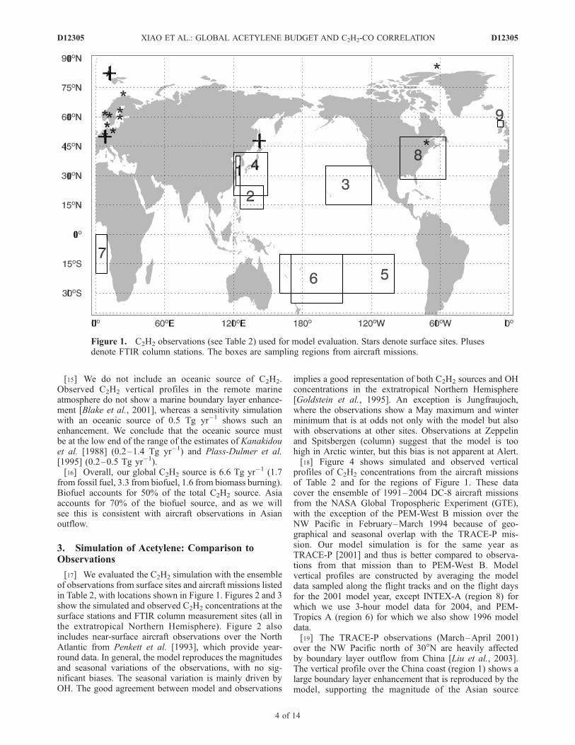
[17] We evaluated the C2H2 simulation with the ensembleof observations from surface sites and aircraft missions listedin Table 2, with locations shown in Figure 1. Figures 2 and 3show the simulated and observed C2H2 concentrations at thesurface stations and FTIR column measurement sites (all inthe extratropical Northern Hemisphere). Figure 2 alsoincludes near-surface aircraft observations over the NorthAtlantic from Penkett et al. [1993], which provide year-round data. In general, the model reproduces the magnitudesand seasonal variations of the observations, with no sig-nificant biases. The seasonal variation is mainly driven byOH. The good agreement between model and observations

implies a good representation of both C2H2 sources and OHconcentrations in the extratropical Northern Hemisphere[Goldstein et al., 1995]. An exception is Jungfraujoch,where the observations show a May maximum and winterminimum that is at odds not only with the model but alsowith observations at other sites. Observations at Zeppelinand Spitsbergen (column) suggest that the model is toohigh in Arctic winter, but this bias is not apparent at Alert.[18] Figure 4 shows simulated and observed vertical

profiles of C2H2 concentrations from the aircraft missionsof Table 2 and for the regions of Figure 1. These datacover the ensemble of 1991–2004 DC-8 aircraft missionsfrom the NASA Global Tropospheric Experiment (GTE),with the exception of the PEM-West B mission over theNW Pacific in February–March 1994 because of geo-graphical and seasonal overlap with the TRACE-P mis-sion. Our model simulation is for the same year asTRACE-P [2001] and thus is better compared to observa-tions from that mission than to PEM-West B. Modelvertical profiles are constructed by averaging the modeldata sampled along the flight tracks and on the flight daysfor the 2001 model year, except INTEX-A (region 8) forwhich we use 3-hour model data for 2004, and PEM-Tropics A (region 6) for which we also show 1996 modeldata.[19] The TRACE-P observations (March–April 2001)

over the NW Pacific north of 30�N are heavily affectedby boundary layer outflow from China [Liu et al., 2003].The vertical profile over the China coast (region 1) shows alarge boundary layer enhancement that is reproduced by themodel, supporting the magnitude of the Asian source

Figure 1. C2H2 observations (see Table 2) used for model evaluation. Stars denote surface sites. Plusesdenote FTIR column stations. The boxes are sampling regions from aircraft missions.


4 of 14

D12305

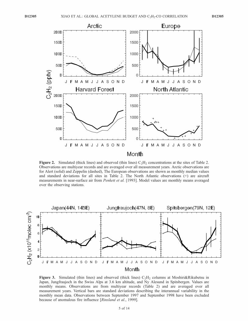
Figure 3. Simulated (thin lines) and observed (thick lines) C2H2 columns at Moshiri&Rikubetsu inJapan, Jungfraujoch in the Swiss Alps at 3.6 km altitude, and Ny Alesund in Spitsbergen. Values aremonthly means. Observations are from multiyear records (Table 2) and are averaged over allmeasurement years. Vertical bars are standard deviations describing the interannual variability in themonthly mean data. Observations between September 1997 and September 1998 have been excludedbecause of anomalous fire influence [Rinsland et al., 1999].

Figure 2. Simulated (thick lines) and observed (thin lines) C2H2 concentrations at the sites of Table 2.Observations are multiyear records and are averaged over all measurement years. Arctic observations arefor Alert (solid) and Zeppelin (dashed), The European observations are shown as monthly median valuesand standard deviations for all sites in Table 2. The North Atlantic observations (+) are aircraftmeasurements in near-surface air from Penkett et al. [1993]. Model values are monthly means averagedover the observing stations.


5 of 14

D12305

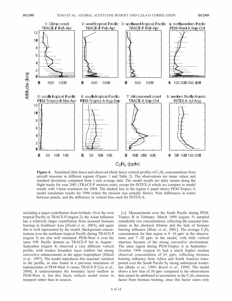
including a major contribution from biofuels. Over the westtropical Pacific in TRACE-P (region 2), the Asian influencehas a relatively larger contribution from seasonal biomassburning in Southeast Asia [Heald et al., 2003], and againthis is well represented by the model. Background concen-trations over the northeast tropical Pacific during TRACE-P(region 3) are also well simulated. PEM-West A over thesame NW Pacific domain as TRACE-P but in August–September (region 4) observed a very different verticalprofile, with weaker boundary layer outflow but strongconvective enhancements in the upper troposphere [Ehhaltet al., 1997]. The model reproduces this seasonal variationin the profile, as also found in a previous simulation ofradionuclides in PEM-West A versus TRACE-P [Liu et al.,2004]. It underestimates the boundary layer outflow inPEM-West A, but this likely reflects model errors intransport rather than in sources.

[20] Measurements over the South Pacific during PEM-Tropics B in February–March 1999 (region 5) sampledremarkably low concentrations, reflecting the seasonal min-imum in the chemical lifetime and the lack of biomassburning influence [Blake et al., 2001]. The average C2H2

concentration for that region is 9–16 pptv in the observa-tions and 7–20 pptv in the model, with little verticalstructure because of the strong convective environment.The same region during PEM-Tropics A in September–October 1996 (region 6) had a much higher medianobserved concentration of 65 pptv, reflecting biomassburning influence from Africa and South America trans-ported over the South Pacific by strong subtropical wester-lies [Blake et al., 1999; Board et al., 1999]. The modelshows a low bias of 30 pptv compared to the observationsthat cannot be attributed to uncertainty in the C2H2 emissionfactor from biomass burning, since this factor varies only

Figure 4. Simulated (thin lines) and observed (thick lines) vertical profiles of C2H2 concentrations fromaircraft missions in different regions (Figure 1 and Table 2). The observations are mean values andstandard deviations computed from 1-min average data. The model results are daily means along theflight tracks for year 2001 (TRACE-P mission year), except for INTEX-A which we compare to modelresults with 3-hour resolution for 2004. The dashed line in the region 6 panel shows PEM-Tropics Amodel simulation results for 1996 (when the mission was actually flown). Note differences in scalesbetween panels, and the difference in vertical bins used for INTEX-A.


6 of 14

D12305

over a narrow range (Table 1), and the model gives asuccessful simulation of C2H2 concentrations in Africanbiomass burning outflow during the TRACE-A aircraft mis-sion in September–October 1992 (region 7 of Figure 4).Amajor factor for the bias appears to be interannual variabilityin transport, as the simulation using 1996meteorology (dashedline) shows a reduction of 18 pptv (i.e., by 60%) in the bias.Meteorological conditions in 1996 were particularly condu-cive to transport of African biomass burning plumes over theSouth Pacific [Fuelberg et al., 1999; Staudt et al., 2002].[21] Also shown in Figure 4 (region 8) are the simulated

and observed vertical profiles of C2H2 over eastern NorthAmerica during the INTEX-A mission (July August 2004).The observed C2H2 concentrations average 145 pptv in theboundary layer and 90 pptv in the free troposphere. Theboundary layer enhancement in the model is due almostexclusively to US fossil fuel emissions; boreal forest fireinfluence is weak and vertically distributed, contributing onaverage 15 pptv to the vertical profile. The model is about30 pptv too low throughout the profile, suggesting a 30%bias in background C2H2 at northern midlatitudes in sum-mer. However, such a bias is not apparent in the surface andcolumn data of Figures 2 and 3.

4. The C2H2-CO Relationship

[22] The aircraft missions in Figure 1 cover differentregions of the world in different seasons. We examine herethe C2H2-CO correlations and linear regressions in thesedifferent data sets and compare to results from the GEOS-Chem simulation. Our goal is to determine the informationcontained in the C2H2-CO relationships for testing model

emissions, transport, and OH levels, and to better interpretthese relationships as markers for air mass age. All linearregressions presented here use the reduced-major-axis meth-od allowing for errors in both variables.

4.1. dC2H2/dCO Regression Slopes and ConcentrationRatios

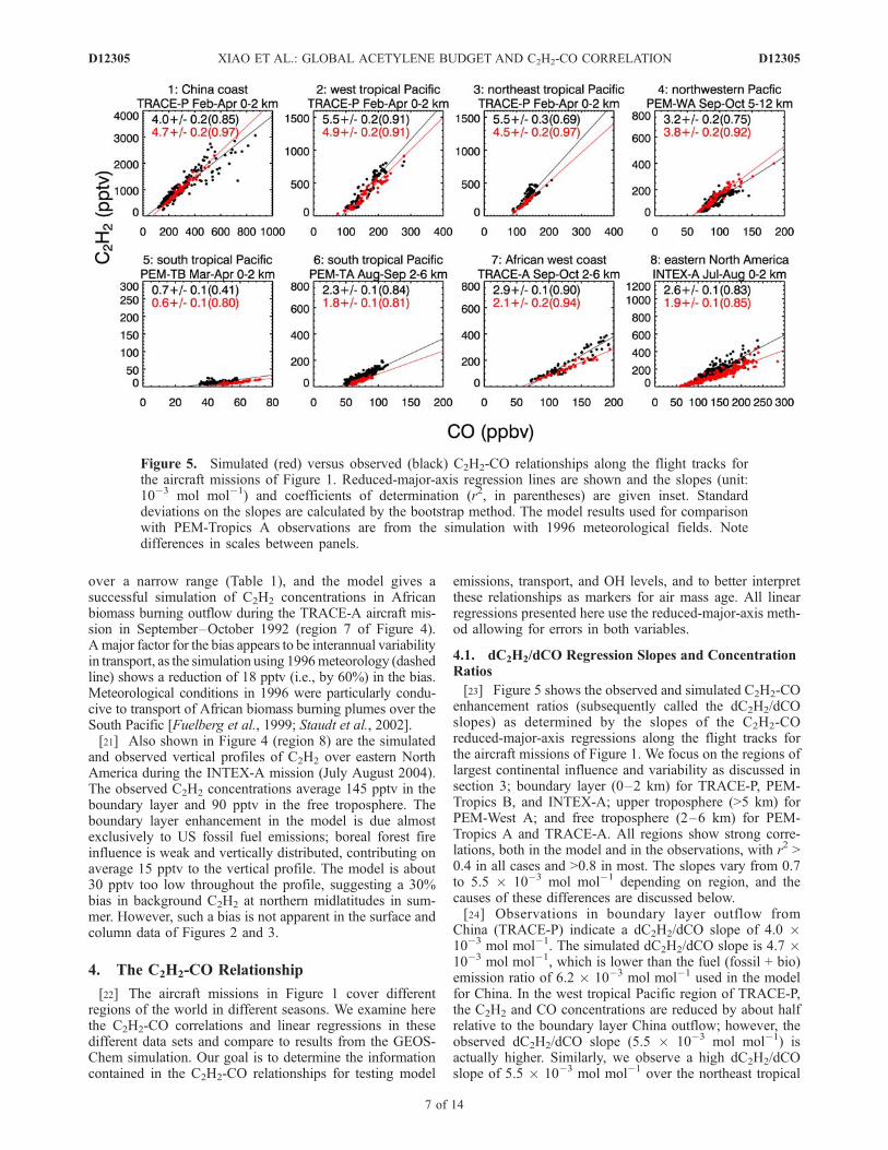
[23] Figure 5 shows the observed and simulated C2H2-COenhancement ratios (subsequently called the dC2H2/dCOslopes) as determined by the slopes of the C2H2-COreduced-major-axis regressions along the flight tracks forthe aircraft missions of Figure 1. We focus on the regions oflargest continental influence and variability as discussed insection 3; boundary layer (0–2 km) for TRACE-P, PEM-Tropics B, and INTEX-A; upper troposphere (>5 km) forPEM-West A; and free troposphere (2–6 km) for PEM-Tropics A and TRACE-A. All regions show strong corre-lations, both in the model and in the observations, with r2 >0.4 in all cases and >0.8 in most. The slopes vary from 0.7to 5.5 � 10�3 mol mol�1 depending on region, and thecauses of these differences are discussed below.[24] Observations in boundary layer outflow from

China (TRACE-P) indicate a dC2H2/dCO slope of 4.0 �10�3 mol mol�1. The simulated dC2H2/dCO slope is 4.7 �10�3 mol mol�1, which is lower than the fuel (fossil + bio)emission ratio of 6.2 � 10�3 mol mol�1 used in the modelfor China. In the west tropical Pacific region of TRACE-P,the C2H2 and CO concentrations are reduced by about halfrelative to the boundary layer China outflow; however, theobserved dC2H2/dCO slope (5.5 � 10�3 mol mol�1) isactually higher. Similarly, we observe a high dC2H2/dCOslope of 5.5 � 10�3 mol mol�1 over the northeast tropical

Figure 5. Simulated (red) versus observed (black) C2H2-CO relationships along the flight tracks forthe aircraft missions of Figure 1. Reduced-major-axis regression lines are shown and the slopes (unit:10�3 mol mol�1) and coefficients of determination (r2, in parentheses) are given inset. Standarddeviations on the slopes are calculated by the bootstrap method. The model results used for comparisonwith PEM-Tropics A observations are from the simulation with 1996 meteorological fields. Notedifferences in scales between panels.


7 of 14

D12305

Pacific during TRACE-P (region 3), although this regionwas remote from continental influence. The model under-estimates the slopes in regions 2 and 3, but it reproduces thequalitative result that the slopes do not decline duringapparent aging. We find that the C2H2-CO correlations inregions 2 and 3 are driven in part by contrast betweentropical air masses with low C2H2 and midlatitude airmasses with high C2H2. A problem with interpretingC2H2-CO correlations to diagnose aging is the assumptionthat the background air anchoring the correlation is the sameas the background air in which the polluted air dilutes. Thatassumption fails for regions 2 and 3.[25] The slope observed over the NW Pacific above 5 km

altitude during PEM-West A in August–September is 3.2 �10�3 mol mol�1, lower than in TRACE-P. The model (3.8�10�3 mol mol�1) reproduces the relatively lower slopeobserved in PEM-West A than in TRACE-P, which canbe attributed mainly to the influence of chemical aging. Thesimulated dC2H2/dCO slope in biomass burning outflowsampled over the African west coast during TRACE-A is2.1 � 10�3 mol mol�1, as compared to the observed slopeof 2.9 � 10�3 mol mol�1. It is lower than in Asian outflowbecause of the relatively low emission ratio from biomassburning (Table 1). A very low slope of 0.7 � 10�3 molmol�1 is observed over the south tropical Pacific duringPEM-Tropics B (region 5), consistent with the model (0.6 �10�3 mol mol�1) and reflecting the extensive aging.[26] PEM-Tropics A observations over the South Pacific

were influenced by biomass burning effluents transportedfrom southern Africa and South America over typicaltimescales of 5–7 days [Fuelberg et al., 1999; Gregory etal., 1999; Staudt et al., 2002]. The median C2H2 concen-tration observed in PEM-Tropics A is about 60% of that inTRACE-A outflow (70 pptv in region 6 versus 128 pptv inregion 7). The observed dC2H2/dCO slope in PEM-TropicsA (2.3 � 10�3 mol mol�1) is similar to that observed inTRACE-A (2.9 � 10�3 mol mol�1). The simulated slopesin PEM-Tropics A and TRACE-A are also close to eachother (1.8 � 10�3 mol mol�1 versus 2.1 � 10�3 molmol�1). Again, this appears to be due to difference betweenthe background in which the biomass burning effluents are

diluting versus the background anchoring the C2H2-COcorrelation, as previously discussed by Mauzerall et al.[1998] for the interpretation of dO3/dCO slopes in agedbiomass burning plumes during TRACE-A. The back-ground C2H2 and CO concentrations (as defined by the10th percentiles of the data sets) are 30 pptv and 55 ppbv inPEM-Tropics A, versus 77 pptv and 85 ppbv in the AfricanWest Coast outflow of TRACE-A.[27] The observed dC2H2/dCO slope in the North American

boundary layer during INTEX-A is 2.6 � 10�3 mol mol�1.The simulated slope is 1.9� 10�3 mol mol�1, reflectingmodelbias in simulating the C2H2 background (see section 3).[28] Figure 6 shows the global distribution of the simu-

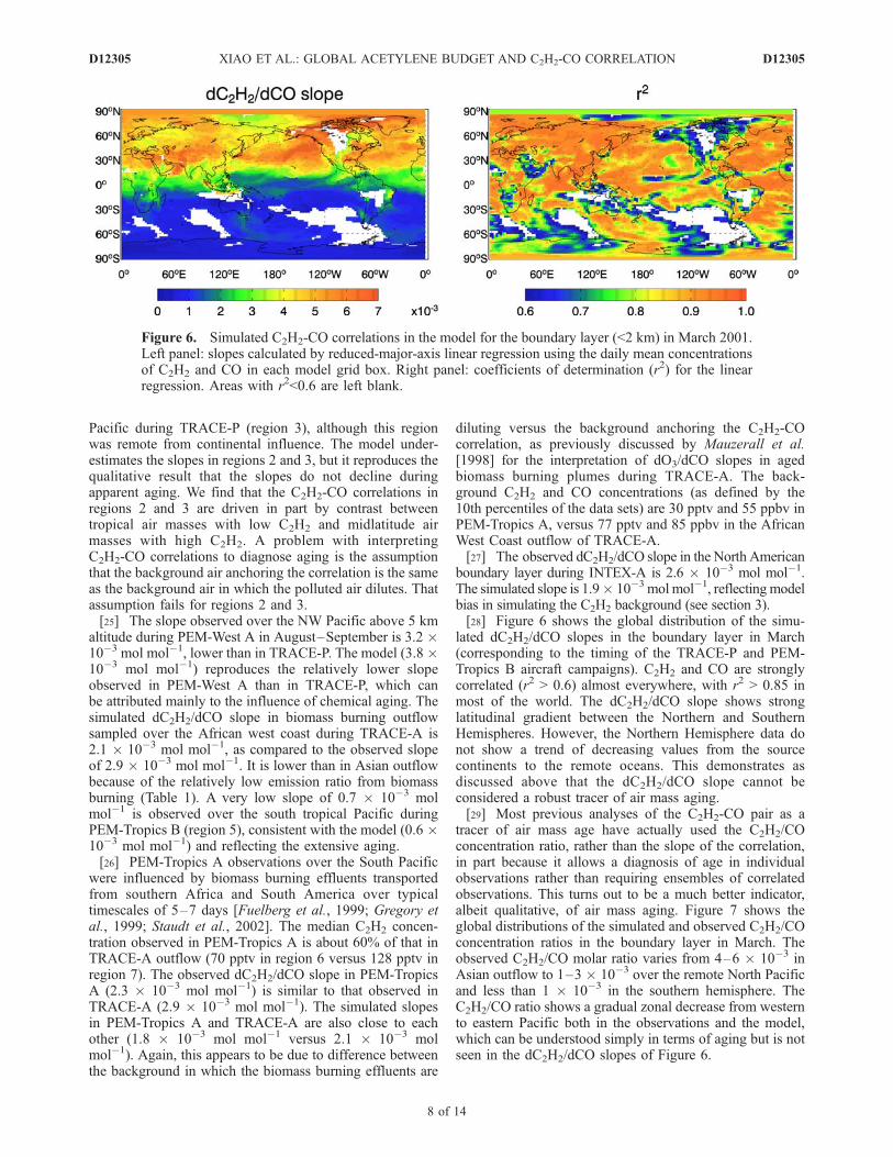
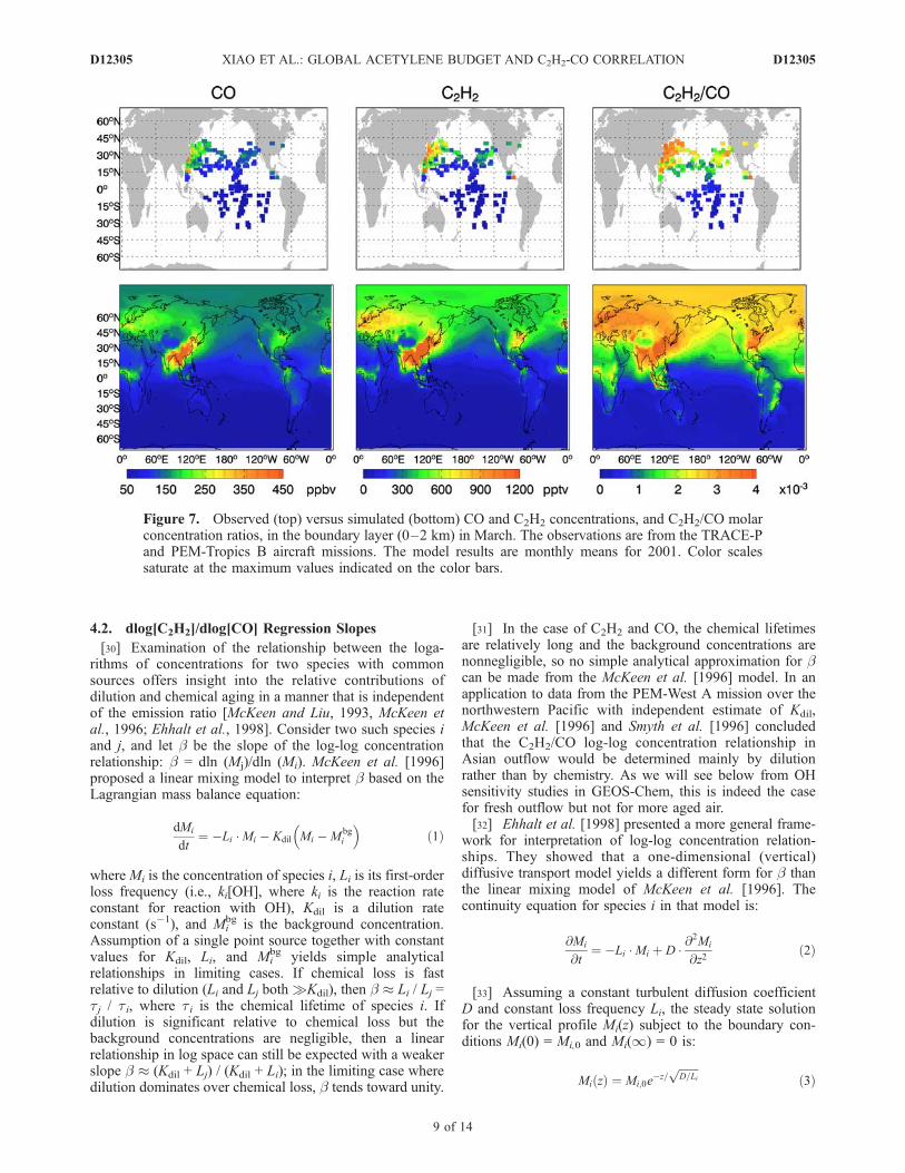
lated dC2H2/dCO slopes in the boundary layer in March(corresponding to the timing of the TRACE-P and PEM-Tropics B aircraft campaigns). C2H2 and CO are stronglycorrelated (r2 > 0.6) almost everywhere, with r2 > 0.85 inmost of the world. The dC2H2/dCO slope shows stronglatitudinal gradient between the Northern and SouthernHemispheres. However, the Northern Hemisphere data donot show a trend of decreasing values from the sourcecontinents to the remote oceans. This demonstrates asdiscussed above that the dC2H2/dCO slope cannot beconsidered a robust tracer of air mass aging.[29] Most previous analyses of the C2H2-CO pair as a

tracer of air mass age have actually used the C2H2/COconcentration ratio, rather than the slope of the correlation,in part because it allows a diagnosis of age in individualobservations rather than requiring ensembles of correlatedobservations. This turns out to be a much better indicator,albeit qualitative, of air mass aging. Figure 7 shows theglobal distributions of the simulated and observed C2H2/COconcentration ratios in the boundary layer in March. Theobserved C2H2/CO molar ratio varies from 4–6 � 10�3 inAsian outflow to 1–3 � 10�3 over the remote North Pacificand less than 1 � 10�3 in the southern hemisphere. TheC2H2/CO ratio shows a gradual zonal decrease from westernto eastern Pacific both in the observations and the model,which can be understood simply in terms of aging but is notseen in the dC2H2/dCO slopes of Figure 6.

Figure 6. Simulated C2H2-CO correlations in the model for the boundary layer (<2 km) in March 2001.Left panel: slopes calculated by reduced-major-axis linear regression using the daily mean concentrationsof C2H2 and CO in each model grid box. Right panel: coefficients of determination (r2) for the linearregression. Areas with r2<0.6 are left blank.


8 of 14

D12305

4.2. dlog[C2H2]/dlog[CO] Regression Slopes

[30] Examination of the relationship between the loga-rithms of concentrations for two species with commonsources offers insight into the relative contributions ofdilution and chemical aging in a manner that is independentof the emission ratio [McKeen and Liu, 1993, McKeen etal., 1996; Ehhalt et al., 1998]. Consider two such species iand j, and let b be the slope of the log-log concentrationrelationship: b = dln (Mj)/dln (Mi). McKeen et al. [1996]proposed a linear mixing model to interpret b based on theLagrangian mass balance equation:

dMi

dt¼ �Li �Mi � Kdil Mi �M

bgi

� �ð1Þ

where Mi is the concentration of species i, Li is its first-orderloss frequency (i.e., ki[OH], where ki is the reaction rateconstant for reaction with OH), Kdil is a dilution rateconstant (s�1), and Mi

bg is the background concentration.Assumption of a single point source together with constantvalues for Kdil, Li, and Mi

bg yields simple analyticalrelationships in limiting cases. If chemical loss is fastrelative to dilution (Li and Lj both �Kdil), then b � Li / Lj =tj / ti, where ti is the chemical lifetime of species i. Ifdilution is significant relative to chemical loss but thebackground concentrations are negligible, then a linearrelationship in log space can still be expected with a weakerslope b � (Kdil + Lj) / (Kdil + Li); in the limiting case wheredilution dominates over chemical loss, b tends toward unity.

[31] In the case of C2H2 and CO, the chemical lifetimesare relatively long and the background concentrations arenonnegligible, so no simple analytical approximation for bcan be made from the McKeen et al. [1996] model. In anapplication to data from the PEM-West A mission over thenorthwestern Pacific with independent estimate of Kdil,McKeen et al. [1996] and Smyth et al. [1996] concludedthat the C2H2/CO log-log concentration relationship inAsian outflow would be determined mainly by dilutionrather than by chemistry. As we will see below from OHsensitivity studies in GEOS-Chem, this is indeed the casefor fresh outflow but not for more aged air.[32] Ehhalt et al. [1998] presented a more general frame-

work for interpretation of log-log concentration relation-ships. They showed that a one-dimensional (vertical)diffusive transport model yields a different form for b thanthe linear mixing model of McKeen et al. [1996]. Thecontinuity equation for species i in that model is:

@Mi

@t¼ �Li �Mi þ D � @

2Mi

@z2ð2Þ

[33] Assuming a constant turbulent diffusion coefficientD and constant loss frequency Li, the steady state solutionfor the vertical profile Mi(z) subject to the boundary con-ditions Mi(0) = Mi,0 and Mi(1) = 0 is:

MiðzÞ ¼ Mi;0e�z=

ffiffiffiffiffiffiffiD=Li

pð3Þ

Figure 7. Observed (top) versus simulated (bottom) CO and C2H2 concentrations, and C2H2/CO molarconcentration ratios, in the boundary layer (0–2 km) in March. The observations are from the TRACE-Pand PEM-Tropics B aircraft missions. The model results are monthly means for 2001. Color scalessaturate at the maximum values indicated on the color bars.


9 of 14

D12305

[34] This model yields a linear log-log relationshipbetween species i and j with slope b ¼

ffiffiffiffiffiffiffiffiffiffiti=tj

p. Ehhalt et

al. [1998] presented illustrative simulations with a three-dimensional CTM indicating that b varies with the relativeimportance of dilution versus photochemical loss. For b = 1,the decline is only due to dilution acting on both species atthe same rate, in the same way as the McKeen et al. [1996]model. b ¼

ffiffiffiffiffiffiffiffiffiffiti=tj

pindicates that dilution and chemical

decay act at comparable rates. b >ffiffiffiffiffiffiffiffiffiffiti=tj

p(where ti > tj)

indicates that chemical decay dominates over dilution. Forthe C2H2-CO pair, the lifetime ratio tCO/tC2H2 remains in anarrow range 3–3.5 (

ffiffiffiffiffiffiffiffiffiffiffiffiffiffiffiffiffiffiffiffiffitCO=tC2H2

pis in the range 1.7–1.9)

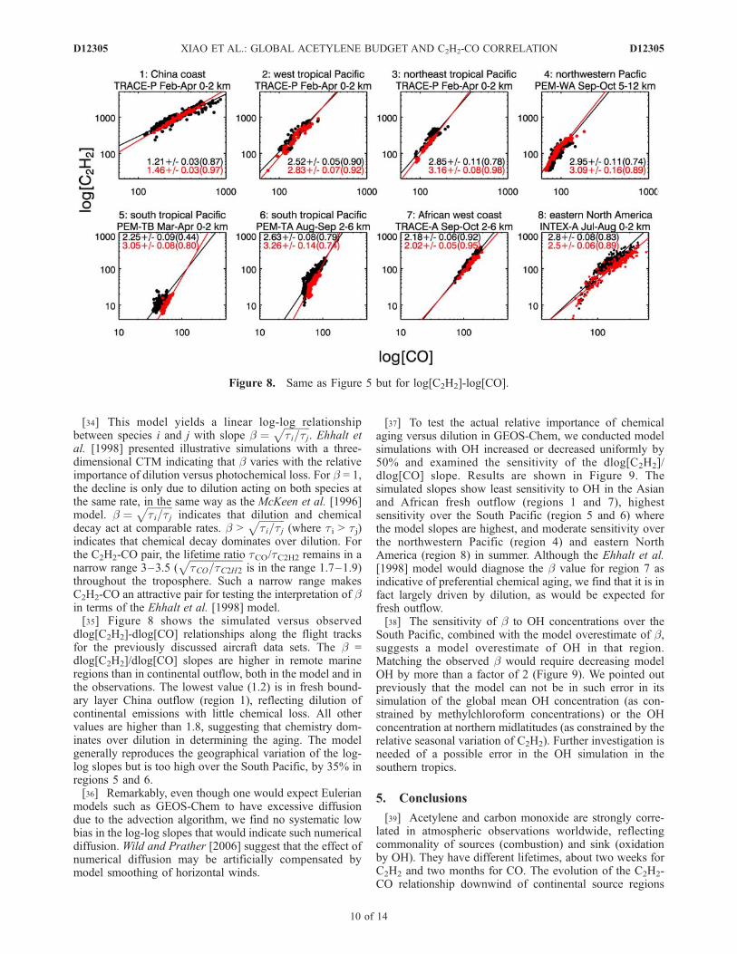
throughout the troposphere. Such a narrow range makesC2H2-CO an attractive pair for testing the interpretation of bin terms of the Ehhalt et al. [1998] model.[35] Figure 8 shows the simulated versus observed

dlog[C2H2]-dlog[CO] relationships along the flight tracksfor the previously discussed aircraft data sets. The b =dlog[C2H2]/dlog[CO] slopes are higher in remote marineregions than in continental outflow, both in the model and inthe observations. The lowest value (1.2) is in fresh bound-ary layer China outflow (region 1), reflecting dilution ofcontinental emissions with little chemical loss. All othervalues are higher than 1.8, suggesting that chemistry dom-inates over dilution in determining the aging. The modelgenerally reproduces the geographical variation of the log-log slopes but is too high over the South Pacific, by 35% inregions 5 and 6.[36] Remarkably, even though one would expect Eulerian

models such as GEOS-Chem to have excessive diffusiondue to the advection algorithm, we find no systematic lowbias in the log-log slopes that would indicate such numericaldiffusion. Wild and Prather [2006] suggest that the effect ofnumerical diffusion may be artificially compensated bymodel smoothing of horizontal winds.

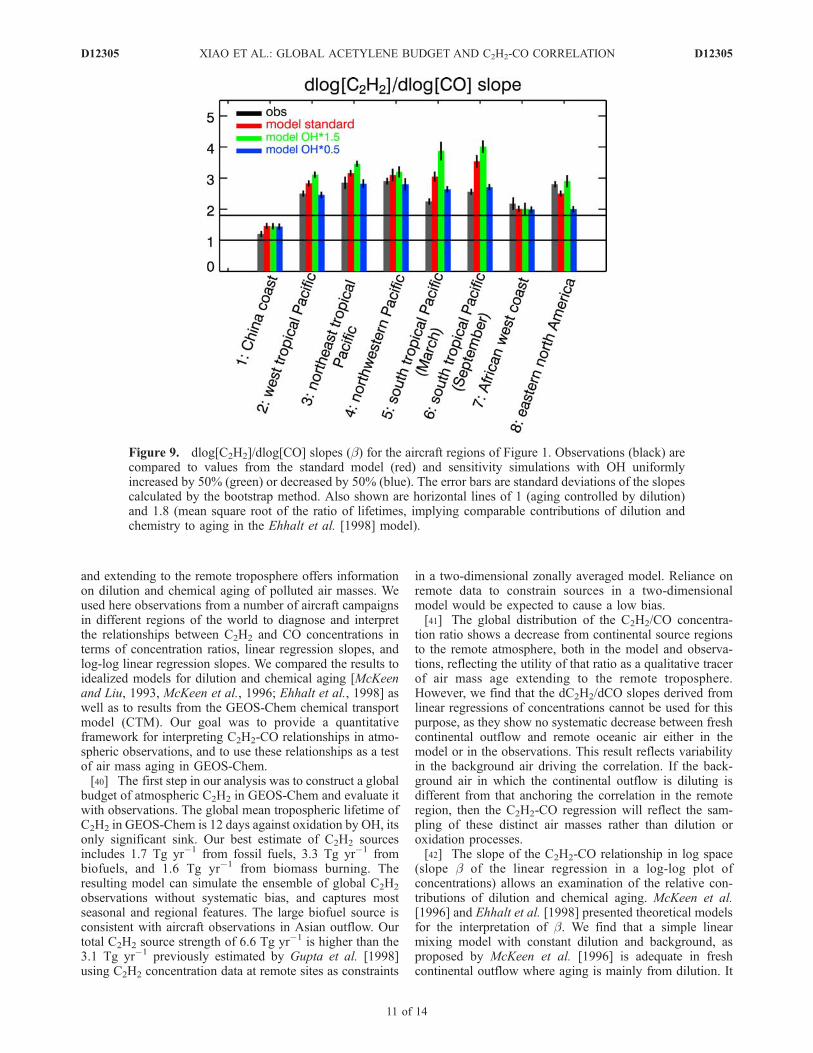
[37] To test the actual relative importance of chemicalaging versus dilution in GEOS-Chem, we conducted modelsimulations with OH increased or decreased uniformly by50% and examined the sensitivity of the dlog[C2H2]/dlog[CO] slope. Results are shown in Figure 9. Thesimulated slopes show least sensitivity to OH in the Asianand African fresh outflow (regions 1 and 7), highestsensitivity over the South Pacific (region 5 and 6) wherethe model slopes are highest, and moderate sensitivity overthe northwestern Pacific (region 4) and eastern NorthAmerica (region 8) in summer. Although the Ehhalt et al.[1998] model would diagnose the b value for region 7 asindicative of preferential chemical aging, we find that it is infact largely driven by dilution, as would be expected forfresh outflow.[38] The sensitivity of b to OH concentrations over the

South Pacific, combined with the model overestimate of b,suggests a model overestimate of OH in that region.Matching the observed b would require decreasing modelOH by more than a factor of 2 (Figure 9). We pointed outpreviously that the model can not be in such error in itssimulation of the global mean OH concentration (as con-strained by methylchloroform concentrations) or the OHconcentration at northern midlatitudes (as constrained by therelative seasonal variation of C2H2). Further investigation isneeded of a possible error in the OH simulation in thesouthern tropics.

5. Conclusions

[39] Acetylene and carbon monoxide are strongly corre-lated in atmospheric observations worldwide, reflectingcommonality of sources (combustion) and sink (oxidationby OH). They have different lifetimes, about two weeks forC2H2 and two months for CO. The evolution of the C2H2-CO relationship downwind of continental source regions

Figure 8. Same as Figure 5 but for log[C2H2]-log[CO].


10 of 14

D12305

and extending to the remote troposphere offers informationon dilution and chemical aging of polluted air masses. Weused here observations from a number of aircraft campaignsin different regions of the world to diagnose and interpretthe relationships between C2H2 and CO concentrations interms of concentration ratios, linear regression slopes, andlog-log linear regression slopes. We compared the results toidealized models for dilution and chemical aging [McKeenand Liu, 1993, McKeen et al., 1996; Ehhalt et al., 1998] aswell as to results from the GEOS-Chem chemical transportmodel (CTM). Our goal was to provide a quantitativeframework for interpreting C2H2-CO relationships in atmo-spheric observations, and to use these relationships as a testof air mass aging in GEOS-Chem.[40] The first step in our analysis was to construct a global

budget of atmospheric C2H2 in GEOS-Chem and evaluate itwith observations. The global mean tropospheric lifetime ofC2H2 in GEOS-Chem is 12 days against oxidation by OH, itsonly significant sink. Our best estimate of C2H2 sourcesincludes 1.7 Tg yr�1 from fossil fuels, 3.3 Tg yr�1 frombiofuels, and 1.6 Tg yr�1 from biomass burning. Theresulting model can simulate the ensemble of global C2H2

observations without systematic bias, and captures mostseasonal and regional features. The large biofuel source isconsistent with aircraft observations in Asian outflow. Ourtotal C2H2 source strength of 6.6 Tg yr�1 is higher than the3.1 Tg yr�1 previously estimated by Gupta et al. [1998]using C2H2 concentration data at remote sites as constraints

in a two-dimensional zonally averaged model. Reliance onremote data to constrain sources in a two-dimensionalmodel would be expected to cause a low bias.[41] The global distribution of the C2H2/CO concentra-

tion ratio shows a decrease from continental source regionsto the remote atmosphere, both in the model and observa-tions, reflecting the utility of that ratio as a qualitative tracerof air mass age extending to the remote troposphere.However, we find that the dC2H2/dCO slopes derived fromlinear regressions of concentrations cannot be used for thispurpose, as they show no systematic decrease between freshcontinental outflow and remote oceanic air either in themodel or in the observations. This result reflects variabilityin the background air driving the correlation. If the back-ground air in which the continental outflow is diluting isdifferent from that anchoring the correlation in the remoteregion, then the C2H2-CO regression will reflect the sam-pling of these distinct air masses rather than dilution oroxidation processes.[42] The slope of the C2H2-CO relationship in log space

(slope b of the linear regression in a log-log plot ofconcentrations) allows an examination of the relative con-tributions of dilution and chemical aging. McKeen et al.[1996] and Ehhalt et al. [1998] presented theoretical modelsfor the interpretation of b. We find that a simple linearmixing model with constant dilution and background, asproposed by McKeen et al. [1996] is adequate in freshcontinental outflow where aging is mainly from dilution. It

Figure 9. dlog[C2H2]/dlog[CO] slopes (b) for the aircraft regions of Figure 1. Observations (black) arecompared to values from the standard model (red) and sensitivity simulations with OH uniformlyincreased by 50% (green) or decreased by 50% (blue). The error bars are standard deviations of the slopescalculated by the bootstrap method. Also shown are horizontal lines of 1 (aging controlled by dilution)and 1.8 (mean square root of the ratio of lifetimes, implying comparable contributions of dilution andchemistry to aging in the Ehhalt et al. [1998] model).


11 of 14

D12305

is inadequate for more remote conditions. Ehhalt et al.[1998] offer a more general model framework for interpret-ing the observed log-log relationships in remote air. In thatmodel, a b value equal to the square root of the ratios ofchemical lifetimes (1.8 for the C2H2-CO pair) indicatescomparable contributions from dilution and chemical aging;lower values of b indicate a dominance from dilution, andhigher values indicate a dominance from chemistry. Thismodel suggests that aging of air in remote regions asdiagnosed by the log[C2H2]-log[CO] relationship is drivenby chemical loss more than by dilution.[43] The GEOS-Chem CTM generally reproduces the

values of b observed for the different regions, in particularthe gradient between continental air and remote oceanic air.Sensitivity simulations with modified OH concentrationsshow that b is insensitive to OH in continental outflow(where aging is controlled by dilution) but sensitive to OHin remote air (where aging is controlled by chemistry).Model values of b are biased high over the South Pacific. Asensitivity simulation with OH concentrations reduced by50% significantly reduces the magnitude of the bias, sug-gesting that model OH concentrations in that region may beoverestimated.

[44] Acknowledgments. This work was funded by the AtmosphericChemistry Program of the US National Science Foundation. We would liketo thank Jennifer Logan, Stuart McKeen, and Bill Munger for helpfuldiscussions. We thank Justus Notholt for providing averaging kernelinformation for column observations of C2H2. We thank Hongyu Liu forhelping to set up the GEOS-Chem simulation for the year 1996. We alsothank Rynda Hudman and Inna Megretskaia for help with processing theC2H2 data from aircraft missions.

ReferencesAndreae, M. O., and P. Merlet (2001), Emission of trace gases and aerosolsfrom biomass burning, Glob. Biogeochem. Cycles, 15(4), 955–966.

Atkinson, R. (2000), Atmospheric chemistry of VOCs and NOx, Atmos.Environ., 34, 2063–2101.

Barletta, B., S. Meinardi, F. S. Rowland, C. Y. Chan, X. M. Wang, S. C.Zou, L. Y. Chan, and D. R. Blake (2005), Volatile organic compounds in43 Chinese cities, Atmos. Environ., 39(32), 5979–5990.

Bertschi, I. T., R. J. Yokelson, D. E. Ward, T. J. Christian, and W. M. Hao(2003), Trace gas emissions from the production and use of domestic bio-fuels in Zambia measured by open-path Fourier transform infrared spectro-scopy, J. Geophys. Res., 108(D13), 8469, doi:10.1029/2002JD002158.

Bey, I., D. J. Jacob, R. M. Yantosca, J. A. Logan, B. Field, A. M. Fiore, Q.Li, H. Liu, L. J. Mickley, and M. Schultz (2001), Global modeling oftropospheric chemistry with assimilated meteorology: Model descriptionand evaluation, J. Geophys. Res., 106, 23,073–23,096.

Blake, D. R., D. F. Hurst, T. W. Smith, W. J. Whipple, T. Y. Chen, N. J.Blake, and F. S. Rowland (1992), Summertime measurements of selectednonmethane hydrocarbons in the Arctic and sub-Arctic during the 1998Arctic Boundary-layer Expedition (ABLE-3A), J. Geophys. Res., 97(D15),16,559–16,588.

Blake, N. J., S. A. Penkett, K. C. Clemitshaw, P. Anwyl, P. Lightman,A. R. W. Marsh, and G. Butcher (1993), Estimates of atmospherichydroxyl radical concentrations from the observed decay of manyreactive hydrocarbons in well-defined urban plumes, J. Geophys.Res., 98(D2), 2851–2864.

Blake, D. R., T. Y. Chen, T. Y. Smith, C. J. L. Wang, O. W. Wingenter, N. J.Blake, F. S. Rowland, and E.W. Mayer (1996), Three-dimensional dis-tribution of nonmenthane hydrocarbons and halocarbons over the north-western Pacific during the 1991 Pacific Exploratory Mission (PEM-WestA), J. Geophys. Res., 101(D1), 1763–1778.

Blake, N. J., et al. (1999), Influence of southern hemispheric biomassburning on midtropospheric distributions of nonmethane hydrocarbonsand selected halocarbons over the remote South Pacific, J. Geophys. Res.,104(D13), 16,213–16,232.

Blake, N. J., et al. (2001), Large-scale latitudinal and vertical distributionsof NMHCs and selected halocarbons in the troposphere over the PacificOcean during the March–April 1999 Pacific Exploratory Mission (PEM-Tropics B), J. Geophys. Res., 106(D23), 32,627.

Blake, N. J., D. R. Blake, B. C. Sive, A. S. Katzenstein, S. Meinardi, O. W.Wingenter, E. L. Atlas, F. Flocke, B. A. Ridley, and F. S. Rowland(2003), The seasonal evolution of NMHCs and light alkyl nitrates atmiddle to high northern latitudes during TOPSE, J. Geophys. Res.,108(D4), 8359, doi:10.1029/2001JD001467.

Board, A. S., H. E. Fuelberg, G. L. Gregory, B. G. Heikes, M. G. Schultz,D. R. Blake, J. E. Dibb, S. T. Sandholm, and R. W. Talbot (1999),Chemical characteristics of air from differing source regions during thePacific Exploratory Mission-Tropics A (PEM-Tropics A), J. Geophys.Res., 104(D13), 16,181–16,196.

Carmichael, G. R., et al. (2003), Evaluating regional emission estimatesusing the TRACE-P observations, J. Geophys. Res., 108(D21), 8810,doi:10.1029/2002JD003116.

de Gouw, J. A., et al. (2005), Budget of organic carbon in a pollutedatmosphere: Results from the New England Air Quality Study in 2002,J. Geophys. Res., 110, D16305, doi:10.1029/2004JD005623.

DeMore, W. B. et al. (1997) Chemical kinetics and photochemical data foruse in stratospheric modeling, JPL Publ. 97-4.

Duncan, B. N., and I. Bey (2004), A modeling study of export pathways ofpollution from Europe: Seasonal and Interannual variations (1987–1997), J. Geophys. Res., 109, D08301, doi:10.1029/2003JD004079.

Duncan, B. N., R. V. Martin, A. C. Staudt, R. Yevich, and J. A. Logan(2003), Interannual and seasonal variability of biomass burning emissionsconstrained by satellite observations, J. Geophys. Res., 108(D2), 4040,doi:10.1029/2002JD002378.

Ehhalt, D. H., F. Rohrer, A. B. Kraus, M. J. Prather, D. R. Blake, and F. S.Rowland (1997), On the significance of regional trace gas distributions asderived from aircraft campaigns in PEM-West A and B, J. Geophys. Res.,102(D23), 28,333–28,351.

Ehhalt, D. H., F. Rohrer, A. Wahner, M. J. Prather, and D. R. Blake (1998),On the use of hydrocarbons for the determination of tropospheric OHconcentrations, J. Geophys. Res., 103(D15), 18,981–18,997.

Fiore, A. M., D. J. Jacob, H. Liu, R. M. Yantosca, T. D. Fairlie, and Q. Li(2003), Variability in surface ozone background over the United States:Implications for air quality policy, J. Geophys. Res., 108, (D24), 4787,doi:10.1029/2003JD003855.

Fishman, J., J. M. Hoell, R. D. Bendura, R. J. McNeil, and V. W. J. H.Kirchhoff (1996), NASA GTE TRACE A experiment (September Octo-ber 1992): Overview, J. Geophys. Res., 101(D19), 23,865–23,879.

Fortin, T. J., B. J. Howard, D. D. Parrish, P. D. Goldan, W. C. Kuster, E. L.Atlas, and R. A. Harley (2005), Temporal changes in US benzene emis-sions inferred from atmospheric measurements, Environ. Sci. Technol.,39(6), 1403–1408.

Fuelberg, H. E., R. E. Newell, S. P. Longmore, Y. Zhu, D. J. Westberg, E. V.Browell, D. R. Blake, G. L. Gregory, and G. W. Sachse (1999), Ameteorological overview of the Pacific Exploratory Mission (PEM) Tro-pics period, J. Geophys. Res., 104(D5), 5585–5622.

Gautrois, M., T. Brauers, R. Koppmann, F. Rohrer, O. Stein, and J. Rudolph(2003), Seasonal variability and trends of volatile organic compounds inthe lower polar troposphere, J. Geophys. Res., 108(D13), 4393,doi:10.1029/2002JD002765.

Goldstein, A. H., S. C. Wofsy, and C. M. Spivakovsky (1995), Seasonalvariations of nonmethane hydrocarbons in rural New England: con-straints on OH concentrations in northern midlatitudes, J. Geophys.Res., 100(D10), 21,023–21,033.

Gregory, G. L., J. T. Merrill, M. C. Shipham, D. R. Blake, G. W. Sachse,and H. B. Singh (1997), Chemical characteristics of tropospheric air overthe Pacific Ocean as measured during PEM-West B: Relationship toAsian outflow and trajectory history, J. Geophys. Res., 102, 28,275–28,285.

Gregory, G. L., et al. (1999), Chemical characteristics of Pacific tropo-spheric air in the region of the Intertropical Convergence Zone and SouthPacific Convergence Zone, J. Geophys. Res., 104(D5), 5677–5696.

Grosjean, E., R. A. Rasmussen, and D. Grosjean (1998), Ambient levels ofgas phase pollutants in Porto Alegre, Brazil, Atmos. Environ., 32(22),3371–3379.

Gupta, M. L., R. J. Cicerone, D. R. Blake, F. S. Rowland, and I. S. A.Isaksen (1998), Global atmospheric distributions and source strengths oflight hydrocarbons and tetrachloroethene, J. Geophy. Res., 103, 28,219–28,235.

Hao, W. M., D. E. Ward, G. Olbu, and S. P. Baker (1996), Emissions ofCO2, CO, and hydrocarbons from fires in diverse African savanna eco-systems, J. Geophys. Res., 101(D19), 23,577–23,584.

Harley, R. A., S. A.McKeen, J. Pearson,M. O. Rodgers, andW. A. Lonneman(2001), Analysis of motor vehicle emissions during the Nashville/MiddleTennessee Ozone Study, J. Geophys. Res., 106(D4), 3559–3567.

Heald, C. L., D. J. Jacob, P. I. Palmer, M. J. Evans, G. W. Sachse, H. B.Singh, and D. R. Blake (2003), Biomass burning emission inventory with


12 of 14

D12305

daily resolution: Application to aircraft observations of Asian outflow,J. Geophys. Res., 108(D21), 8811, doi:10.1029/2002JD003082.

Heald, C. L., D. J. Jacob, D. B. A. Jones, P. I. Palmer, J. A. Logan, D. G.Streets, G. W. Sachse, J. C. Gille, R. N. Hoffman, and T. Nehrkorn(2004), Comparative inverse analysis of satellite (MOPITT) and aircraft(TRACE-P) observations to estimate Asian sources of carbon monoxide,J. Geophys. Res., 109, D23306, doi:10.1029/2004JD005185.

Hegg, D. A., L. F. Radke, P. V. Hobbs, R. A. Rasmussen, and P. J. Riggan(1990), Emissions of some tracer gases from biomass fires, J. Geophys.Res., 95(D5), 5669–5675.

Hoell, J. M., D. Davis, S. C. Liu, R. Newell, M. Shipham, H. Akimoto, R. J.McNeal, R. J. Bendura, and J. W. Drewry (1996), Pacific exploratoryMission-West A (PEM-West A): September–October 1991, J. Geophys.Res., 101(D1), 1641–1653.

Hoell, J. M., D. D. Davis, D. J. Jacob, M. O. Rodgers, R. E. Newell, H. E.Fuelberg, R. J. McNeal, J. L. Raper, and R. J. Bendura (1999), PacificExploratory Mission in the tropical Pacific: PEM-Tropics A, August–September 1996, J. Geophys. Res., 104(D5), 5567–5583.

Hudman, R. C., et al. (2007), Surface and lightning sources of nitrogenoxides over the United States: magnitudes, chemical evolution, and out-flow, J. Geophys. Res., 112, D12505, doi:10.1029/2006JD007912.

Jacob, D. J., J. H. Crawford, M. M. Kleb, V. S. Connors, R. J. Bendura, J. L.Raper, G. W. Sachse, J. C. Gille, L. Emmons, and C. L. Heald (2003),The Transport and Chemical Evolution over the Pacific (TRACE-P) air-craft mission: design, execution, and first results, J. Geophys. Res.,108(D20), 9000, doi:10.1029/2002JD003276.

Jaegle, L., D. A. Jaffe, H. U. Price, P. Weiss-Penzias, P. I. Palmer, M. J.Evans, D. J. Jacob, and I. Bey (2003), Sources and budgets for CO andO3 in the Northeastern Pacific during the spring of 2001: Results fromthe PHOBEA-II Experiment, J. Geophys. Res., 108(D20), 8802,doi:10.1029/2002JD003121.

Kanakidou, M., B. Bonsang, J. C. Le Roulley, G. Lambert, D. Martin, andG. Sennequier (1988), Marine source of atmospheric acetylene, Nature,333(6168), 51–52.

Laurila, T., and H. Hakola (1996), Seasonal cycle of C2–C5 hydrocarbonsover the Baltic Sea and Northern Finland, Atmos. Environ., 30(10–11),1597–1607.

Liang, Q., L. Jaegle, D. A. Jaffe, P. Weiss-Penzias, A. Heckman, and J. A.Snow (2004), Long-range transport of Asian pollution to the northeastPacific: Seasonal variations and transport pathways of carbon monoxide,J. Geophys. Res., 109(D23), D23S07, doi:10.1029/2003JD004402.

Lin, S. J., and R. B. Rood (1996), Multidimensional flux-form semi-Lagrangian transport schemes, Mon. Weather Rev., 124(9), 2046–2070.

Liu, H., D. J. Jacob, I. Bey, R. M. Yantosca, B. N. Duncan, and G. W.Sachse (2003), Transport pathways for Asian combustion outflow overthe Pacific: Interannual and seasonal variations, J. Geophys. Res.,108(D20), 8786, doi:10.1029/2002JD003102.

Liu, H., D. J. Jacob, J. E. Dibb, A. M. Fiore, and R. M. Yantosca (2004),Constraints on the sources of tropospheric ozone from 210Pb–7Be–O3

correlations, J. Geophys. Res., 109, D07306, doi:10.1029/2003JD003988.Mahieu, E., R. Zander, L. Delbouille, P. Demoulin, G. Roland, andC. Servais (1997), Observed trends in total vertical column abundancesof atmospheric gases from IR solar spectra recorded at the Jungfraujoch,J. Atmos. Chem., 28(1–3), 227–243.

Mauzerall, D. L., J. A. Logan, D. J. Jacob, B. E. Anderson, D. R. Blake,J. D. Bradshaw, B. Heikes, G. W. Sachse, H. Singh, and B. Talbot (1998),Photochemistry in biomass burning plumes and implications for tropo-spheric ozone over the tropical South Atlantic, J. Geophys. Res.,103(D7), 8401–8423.

McKeen, S. A., and S. C. Liu (1993), Hydrocarbon ratios and photoche-mical history of air masses, Geophys. Res. Lett., 20(21), 2363–2366.

McKeen, S. A., S. C. Liu, E. Y. Hsie, X. Lin, J. D. Bradshaw, S. Smyth,G. L. Gregory, and D. R. Blake (1996), Hydrocarbon ratios during PEM-WEST A: A model perspective, J. Geophys. Res., 101(D1), 2087–2109.

Moorthi, S., and M. J. Suarez (1992), Relaxed Arakawa-Schubert: A para-meterization of moist convection for general circulation models, Mon.Weather Rev., 120, 978–1002.

Notholt, J., G. Toon, F. Stordal, S. Solberg, N. Schmidbauer, E. Becker, A.Meier, and B. Sen (1997), Seasonal variations of atmospheric trace gasesin the high Arctic at 79 degrees N, J. Geophys. Res., 102(11D), 12,855–12,861.

Olivier, J. G. J., et al. (1996) Description of EDGAR Version 2.0, RIVM/TNO report 771060002, RIVM, Bilthoven, December.

Palmer, P. I., D. J. Jacob, D. B. Jones, C. L. Heald, R. M. Yantosca, J. A.Logan, G. W. Sachse, and D. G. Streets (2003), Inverting for emissions ofcarbon monoxide from Asia using aircraft observations over the westernPacific, J. Geophys. Res., 108(D21), 8828, doi:10.1029/2003JD003397.

Parrish, D. D. (2006), Critical evaluation of US on-road vehicle emissioninventories, Atmos. Environ., 40, 2288–2300.

Parrish, D. D., C. J. Hahn, E. J. Williams, R. B. Norton, F. C. Fehsenfeld,H. B. Singh, J. D. Shetter, B. W. Gandrud, and B. A. Ridley (1992),Indications of photochemical histories of Pacific air masses from mea-surements of atmospheric trace species at Point Arena, California,J. Geophys. Res., 97, 15,883–15,901.

Parrish, D. D., Y. Kondo, O. R. Cooper, C. A. Brock, D. A. Jaffe,M. Trainer, T. Ogawa, G. Hubler, and F. C. Fehsenfeld (2004), Intercon-tinental Transport and Chemical Transformation 2002 (ITCT 2K2) andPacific Exploration of Asian Continental Emission (PEACE) experi-ments: An overview of the 2002 winter and spring intensives, J. Geophys.Res., 109(D23), 111, D23S01, doi:10.1029/2004JD004980.

Penkett, S. A., N. J. Blake, P. Lightman, A. R. W. Marsh, P. Anwyl, andG. Butcher (1993), The seasonal variation of nonmethane hydrocarbonsin the free troposphere over the North Atlantic Ocean: Possible evidencefor extensive reaction of hydrocarbons with the nitrate radical, J. Geo-phys. Res., 98(D2), 2865–2885.

Pierson, W. R., A. W. Gertler, N. F. Robinson, J. C. Sagebiel, B. Zielinska,G. A. Bishop, D. H. Stedman, R. B. Zweidinger, and W. D. Ray (1996),Real-world automotive emissions—Summary of studies in the FortMcHenry and Tuscarora Mountain Tunnels, Atmos. Environ., 30(12),2233–2256.

Plass-Dulmer, C., R. Koppmann, M. Ratte, and J. Rudolph (1995), Lightnonmethane hydrocarbons in seawater, Glob. Biogeochem. Cycles, 9,79–100.

Prinn, R. G., et al. (2001), Evidence for substantial variations of atmo-spheric hydroxyl radical in the past two decades, Science, 292, 1882–1887.

Raper, J. L., M. M. Kleb, D. J. Jacob, D. D. Davis, R. E. Newell, H. E.Fuelberg, R. J. Bendura, J. M. Hoell, and R. J. McNeal (2001), PacificExploratory Mission in the tropical Pacific: PEM-Tropics B, March-April1999, J. Geophys. Res., 106(D23), 32,401–32,425.

Rinsland, C. P., et al. (1999), Infrared solar spectroscopic measurements offree tropospheric CO, C2H6, and HCN above Mauna Loa, Hawaii: Sea-sonal variations and evidence for enhanced emissions from the SoutheastAsian tropical fires of 1997–1998, J. Geophys. Res., 104, 18,667–18,680.

Russo, R. S., et al. (2003), Chemical composition of Asian continentaloutflow over the western Pacific: Results from Transport and ChemicalEvolution over the Pacific (TRACE-P), J. Geophys. Res., 108(D20),8804, doi:10.1029/2002JD003184.

Sigsby, J. E., S. T. Jr., W. Ray, J. M. Lang, and J. W. Duncan (1987),Volatile organic compound emissions from 46 in-use passenger cars,Environ. Sci. Technol., 21, 466–475.

Singh, H. B., W. H. Brune, J. H. Crawford, and D. J. Jacob (2006), Over-view of the summer 2004 Intercontinental Chemical Transport Experi-ment-North America (INTEX-A), J. Geophys. Res., 111, D24501,doi:10.1029/2006JD007905.

Smyth, S., et al. (1996), Comparison of free tropospheric western Pacific airmass classification schemes for the PEM-West A experiment, J. Geophys.Res., 101(D1), 1743–1762.

Solberg, S., C. Dye, N. Schmidbauer, A. Herzog, and G. Gehrig (1996),Carbonyls and nonmethane hydrocarbons at rural European sites from theMediterranean to the Arctic, J. Atmos. Chem., 25(1), 33–66.

Staudt, A. C., D. J. Jacob, J. A. Logan, D. Bachiochi, T. N. Krishnamurti,and N. Poisson (2002), Global chemical model analysis of biomass burn-ing and lightning influences over the South Pacific in austral spring,J. Geophys. Res., 107(D14), 4200, doi:10.1029/2000JD000296.

Streets, D. G., et al. (2003), An inventory of gaseous and primary aerosolemissions in Asia in the year 2000, J. Geophys. Res., 108(D21), 8809,doi:10.1029/2002JD003093.

Swanson, A. L., N. J. Blake, E. Atlas, F. Flocke, D. R. Blake, and F. S.Rowland (2003), Seasonal variations of C2–C4 nonmethane hydrocar-bons and C1–C4 alkyl nitrates at the Summit research station in Green-land, J. Geophys. Res., 108(D2), 4065, doi:10.1029/2001JD001445.

Turquety, S., et al. (2007), Inventory of boreal fire emissions forNorth America in 004: The importance of peat burning and pyro-convective injection, J. Geophys. Res., 112, D12503, doi:10.1029/2006JD007281.

Wang, T., A. J. Ding, D. R. Blake, W. Zahorowski, C. N. Poon, and Y. S. Li(2003), Chemical characterization of the boundary layer outflow of airpollution to Hong Kong during February–April 2001, J. Geophys. Res.,108(D20), 8787, doi:10.1029/2002JD003272.

Wild, O., and M. J. Prather (2006), Global tropospheric ozone modeling:quantifying errors due to grid resolution, J. Geophys. Res., 111, D11305,doi:10.1029/2005JD006605.

Wofsy, S. C., et al. (1992), Atmospheric chemistry in the Arctic and sub-Arctic: Influence of natural fires, industrial emissions, and stratosphericinputs, J. Geophys. Res., 97(D15), 16,731–16,746.


13 of 14

D12305

Yokelson, R. J., I. T. Bertschi, T. J. Christian, P. V. Hobbs, D. E. Ward, andW. M. Hao (2003), Trace gas measurements in nascent, aged, and cloud-processed smoke from African savanna fires by airborne Fourier trans-form infrared spectroscopy (AFTIR), J. Geophys. Res., 108(D13), 8478,doi:10.1029/2002JD002322.

Zhao, Y., et al. (2002), Spectroscopic measurements of tropospheric CO,C2H6, C2H2, and HCN in northern Japan, J. Geophys. Res., 107(D18),4343, doi:10.1029/2001JD000748.

��D. J. Jacob, S. Turquety, and Y. Xiao, Department of Earth and Planetary

Sciences and Division of Engineering and Applied Sciences, HarvardUniversity, Cambridge, MA, USA. ([email protected])


14 of 14

D12305

atmospheric acetylene and its relationship with co as an...

Documents