Atmospheric greenhouse gases

monitoring in India

Yogesh K. Tiwari

Indian Institute of Tropical Meteorology (IITM), Pune

India has one of the largest and fastest growing economies in South Asia and is emerging as a

major contributor to CO2 emissions among developing nations.

Uncertainty of estimated emissions of CO2 over above Asian region are larger due to the lack of

sufficient CO2 monitoring ( Schuck et al., 2010; Peylin et al., 2012; Patra et al, 2013).

Towards a better understanding of CO2 transport pathways, CO2 sources and sinks over Indian

subcontinent, need dense network and high quality CO2 monitoring supplemented by a robust

modeling techniques (Bhattacharya et al., 2009;Tiwari et al., 2011, 2014; Ravi et al., 2014).

CO2 emissions from India

CO2 emissions due to fossil fuel and cement

production over South Asia during 1990-2009

(Source: Boden et al,2011)

Le Quéré et al 2013; Global Carbon Project (GCP) 2013

0

1

2

CO2 emissions (GtC/yr)

(Source: Patra et al, 2013)

Major fluxes of CO2, CH4, N2O

and related species in the

South Asian region

zonal mean of CO2 observed over India

(zonal average) Detrended CO2

AIRS CO2 -Source (NASA)

Zonal average(65°E-100°E) of satellite

retrieved over India is shows monotonous

increase at each latitude band.

Satellite retrievals is shows almost 24ppm

of CO2 increase with an average growth rate

of 2 ppm/yr during 2003-2011 over Indian

region.

Zonal average satellite de-trended CO2

shows clear seasonality from year to year.

CO2 from space (satellite)

Greenhouse gases monitoring techniques we use

1)Discrete

2) In-situ

Greenhouse gases monitoring platforms we work

1)Surface

2)Aircraft

3)Ship

1) Surface sites:

SNG

CRI

DJI

Sinhagad (SNG) – Yogesh Tiwari

(2009 – continue)

Cape Rama (CRI) – Marcel

(1993-2002, 2009-2013)

Darjeeling (DJI) – Anita, Bristol Univ

(2010- 2013)

(SNG)

(SNG)

Surface monitoring site SNG, Pune, India

Wet condition Dry condition

Flask sampling unit

Methodology and analysis techniques

Met sensors and Intet pump

Continuous in-situ measurements of

CO2, CH4, H2O at Sinhagad (SNG)

site

Surface Sensitivity [ppm/(µmol m-2 s-1)]

SNG, Jan

SNG,Jul

CO2 sources at the observation sites based on Lagrangian modeling

Surface Sensitivity

Surface Sensitivity Trajectory

Trajectory

Although the particles are transported from the western part of Asia in January, they are primarily transported

by the northeasterly winds within the planetary boundary layer (PBL) over India as they reach SNG.

Impact of marine layer CO2 fluxes is rather significant on the receptor at SNG.

Ref : Yogesh K.Tiwari, V. Valsala, R. K. Vellore, and K. Ravi Kumar (2013): Effectiveness of surface monitoring stations in capturing regional CO2 emissions

over India. Climate Research, 56, 121-129.

Surface Sensitivity [ppm/(µmol m-2 s-1)]

CRI, Jan

CRI,Jul

Cape Rama

During January, higher surface sensitivity is seen over the central and east coast of India as well as over

the foothills of the Himalayas. In contrast, the surface sensitivity magnitudes are significant over the central

Arabian Sea in July.

The concentrations can be more sensitive to local terrestrial (marine/oceanic) fluxes in January (July).

Ref : Yogesh K.Tiwari, V. Valsala, R. K. Vellore, and K. Ravi Kumar (2013): Effectiveness of surface monitoring stations in capturing regional CO2 emissions

over India. Climate Research, 56, 121-129.

NDVI

Rainfall

Seasonal cycle of NDVI (Normalized Difference Vegetation Index)

and Rainfall at SNG and CRI

NDVI shows a minimum value at SNG to represent

bare soil during April to May, which contrasts the

maximum in October to represent the loss of

vegetation canopy.

Although the NDVI magnitude at CRI is larger, the

month-to-month variability in the vegetation cover is

found to be weaker at CRI as compared to SNG. This

suggests that crop harvesting in the vicinity of SNG

appears to play a role ahead of the summer monsoon

season.

The annual cycle of vegetation at both sites follows

the annual cycle of rainfall.

SNG

CRI

CRI

SNG

SNG

CRI

375

380

385

390

395

400

405

410

415

420

425

04.02.11

25.03.11

22.04.11

20.05.11

17.06.11

15.07.11

12.08.11

09.09.11

04.11.11

23.12.11

20.01.12

09.03.12

13.04.12

11.05.12

15.06.12

27.07.12

07.09.12

12.10.12

16.11.12

21.12.12

08.02.13

15.03.13

19.04.13

25.05.13

21.06.13

19.07.13

16.08.13

13.09.13

11.10.13

08.11.13

06.12.13

SNG - CO2 (ppm)

1600

1650

1700

1750

1800

1850

1900

1950

2000

2050

2100

2150

2200

04.02.11

25.03.11

22.04.11

20.05.11

17.06.11

15.07.11

12.08.11

09.09.11

04.11.11

23.12.11

20.01.12

09.03.12

13.04.12

11.05.12

15.06.12

27.07.12

07.09.12

12.10.12

16.11.12

21.12.12

08.02.13

15.03.13

19.04.13

25.05.13

21.06.13

19.07.13

16.08.13

13.09.13

11.10.13

08.11.13

06.12.13

SNG- CH4 (ppb)

Results:

GHGs observations at

Sinhagad (SNG)

monitoring site

(2011-2013)

Climatological mean of

Observed CH4 & CO2 concentrations.

Comparison with northern and

Southern hemisphere global

Monitoring sites

CO

2 (

pp

m)

(20

10

-201

3)

CO

2 (

pp

m)

(19

93

-200

2)

- CRI

- SNG

SN

G C

RI

CH4 observations and comparisons

with model simulation at three

Observational sites in India

SNG

CRI

DJI

Annual cycle of all-India monthly mean

Vegetation index (NDVI) during

drought and flood years over the

period 1981–2000

Annual cycle of CO2 (ppm)

superimposed with annual cycle of

Rainfall (mm) over Cape Rama based

on the data for 1993-2002

(Ref.: Yogesh K. Tiwari, J. V. Revadekar, K. Ravi Kumar,

2013, Variations in atmospheric Carbon Dioxide and its

association with rainfall and vegetation over India.

Atmospheric Environment, Vol.68 (2013), pp 45-51, DOI:

10.1016/j.atmosenv.2012.11.040)

(Ref.: J. V. Revadekar, Yogesh K. Tiwari, K. Ravi Kumar,

2012, Impact of climate variability on NDVI over Indian

region during1981-2000. International Journal of Remote

Sensing, Vol.33, No.22, 2012, 132-7150, DOI:

10.1080/01431161.2012.697642)

CRI

There is a smaller CO2

variability (8–10 ppm) during

summer monsoon months

(JJAS) compared to values

greater than 15 ppm for the

remainder of the year. This is

in part due to higher

vegetation cover in these months

due to intermittent

precipitation spells.

The observational record also

indicated larger variances

seen at SNG during

post-monsoon months (later than

September) than seen at CRI.

Yogesh K. Tiwari, Ramesh K. Vellore, K Ravi Kumar, Marcel Vander Schoot, and Chun-Ho Cho (2014) Influence of

monsoons on atmospheric CO2 spatial variability and ground-based monitoring over India. Science of the Total

Environment 490 (2014) 570–578.

CO2 variability at SNG and CRI observing sites

Carbon flux

Measurement

Netwrok in

India

(FLUXNET)

-IITM operates

Six sites for

Carbon flux

Measurements

In India

Carbon flux measurement (fluxnet): • Multi-level instrumentation

1. Eddy Covariance (EC) systems at two levels consisting of fast-response 3D sonic

anemometer-thermometer, closed-path CO2-H2O analyzer and data logger

2. soil temperature sensor at 5 levels

3. heat flux plates at 2 levels

4. multi-component weather sensors at 4 levels

5. infra-red thermometer

6. Photosynthetic Active Radiation (PAR) quantum sensor

7. net radiometer

Credits: Pramit

2) Airborne GHGs monitoring: 2010, 2014, 2015

• Instrumentation

•Cavity Ring Down Spectroscopy

(CRDS) for measuring CO2, CH4,

CO, H2O concentrations in the air

•CRDS is a linear optical absorption technique for measuring trace levels of a target

compound in air

•Linear optical absorption technique is a process of passing light through a gas sample

and measuring the amount of light absorbed.

CRDS instrument Data display

Calibrations……..

Credits: Thara P.

Calibration and post-processing:

• Three standards, from WMO certified lab NOAA ESRL USA, are

used to calibrate observations

• Calibration is done at the ground before airborne observations

•Output data are stored at every two second interval

• Post-processing is done with the help of co-located met data

from other instruments

0

2

4

6

0.05 0.10 0.15 0.20 370 380 390 1.75 1.80 1.85 0.1 1 10

CO (ppm)

He

igh

t (k

m)

CO2(ppm) CH

4 (ppm) H

2O (ppm)

Vertical profile during a flight Calibrating in the field

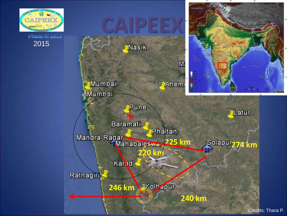
225 km

240 km

274 km220 km

246 km

CAIPEEX 20152015

Credits: Thara P.

Relationship between in-situ CO pollution and

Cloud droplet number concentration over Arabian

sea and inland

Polluted clouds Polluted

No clouds

Clean

No clouds

Clean area

shallow

clouds

Observatio

n height

(m)

Credits: Thara P.

Source: Carl Brenninkmeijer, Max Planck

Schuck et al., 2010, ACP

CruiseTrack and mean CO2 (ppm;

shaded) of the cruise period from

Carbon Tracker model

Land-ocean contrast of surface CO2

The spatial pattern of mean

CO2 from the CarbonTracker

simulations averaged from the

start to the end of the cruise

period.

The sharp land-ocean

contrast in atmospheric CO2 at

the surface (1000 hPa) can be

seen in the CarbonTracker

simulations.

Ref: K. Ravi Kumar., Y. K. Tiwari, V. Valsala, and R. Murtugudde (2014); On understanding of land-ocean contrast of atmospheric CO2 over Bay of Bengal: A

case study during 2009 summer monsoon (Environmental Science and Pollution Research )

3) GHGs monitoring at the ship deck :

Comparison of observations and model simulations over Bay of Bengal

a) b)

c) d)

The land –ocean contrast is observed in the observations of CO2

over BoB. such land-ocean contrast in CO2 prevails during the same

period of every year.

Ref: K. Ravi Kumar., Y. K. Tiwari, V. Valsala, and R. Murtugudde (2014); On understanding of land-ocean contrast of atmospheric CO2 over Bay of Bengal: A

case study during 2009 summer monsoon (Environmental Science and Pollution Research )

Fossil Fuel Bio tracers a

c

b

d

a

c

b

d

The peaks seen here are clearly contributed by the terrestrial

biospheric fluxes (BIO) and fossil fuel (FF), and this also confirms that

the land-ocean contrast is induced by the terrestrial vs. oceanic CO2

fluxes.

Monsoon atmospheric circulation plays a pivotal role in advecting the

CO2 fluxes from the land towards the ocean.

Open ocean – a) 19.07.09 and b) 21.07.09

Coastal ocean - c) 11.08.09 and d) 12.08.09

Ref: K. Ravi Kumar., Y. K. Tiwari, V. Valsala, and R. Murtugudde (2014); On understanding of land-ocean contrast of atmospheric CO2 over Bay of Bengal: A

case study during 2009 summer monsoon (Environmental Science and Pollution Research )

Carbon Tracker CO2

Korean team visited IITM Pune: (MoU between MoES and KMA)

• KMA scientists and engineers visited IITM Gas Chromatograph (GC) lab during

19-23 Sept.2015

•Worked on CO2 and CH4 monitoring at the IITM GC lab

•Monitoring of Sulfur Hexafluoride (SF6) and Nitrous Oxide (N2O) at Gas

Chromatograph (GC) lab at the IITM Pune.

• Collaborations on GHG’s monitoring in India

Inter-comparison of CH4 calibration standards:

Korea (KMA) - India (IITM) - Japan (JMA)

In the intercomparison project, two cylinders containing air of known CH4 mole

fractions are circulated among above participants

New observational sites – starting early next year

72m

20m

Sagar

Cape Rama

Thank You !!