Atmospheric Modeling with High-OrderFinite-Volume Methods

by

Paul Aaron Ullrich

A dissertation submitted in partial fulfillmentof the requirements for the degree of

Doctor of Philosophy(Atmospheric and Space Sciences and Scientific Computing)

in The University of Michigan2011

Doctoral Committee:

Professor Christiane Jablonowski, ChairProfessor Smadar KarniProfessor Richard RoodProfessor Bram van Leer

c© Paul Aaron Ullrich 2011

All Rights Reserved

To Youna

ii

ACKNOWLEDGEMENTS

Throughout the years there have been numerous people who have helped bring

this thesis to fruition. I would like to extend a special thank you to my advisor,

Christiane Jablonowski for her support and insight into both the mathematics and

science of atmospheric dynamics. Another special thank you goes to Bram van Leer

for his seemingly unbounded knowledge on computational fluid dynamics. His insight

and support made the development of this work significantly easier. In addition,

many thanks go to Smadar Karni and Ricky Rood, both of whom have offered unique

insights and perspectives during the development of this project.

I would also like to offer thanks to the many collaborators I have had the pleasure

of working with for the past four years, in particular Peter Lauritzen at NCAR and

Phil Colella at Lawrence Berkeley Lab. I look forward to working with them in the

future.

A special mention goes to all the friends I have met at the University of Michigan,

who have made for many enjoyable experiences both inside and outside the office. I’d

like to give a shout out to Kevin, Ahmed, Jacob, Dan, Kristen, Sid, Matt and many

others who have all been close friends and good company. All of you helped me keep

my sanity in these few years.

Most importantly, I would like to thank my family for all of their support and

encouragement. A special thank you goes to my father, who unfortunately will not

be able to see my graduation – I can honestly say that by accepting nothing short

of the best he led me to where I am today. Of course, thanks go to my mom for

iii

her consistent encouragement and valuable teachings. I would also like to thank my

brother Chris, whose lectures in calculus to me while I was still in elementary school

drove my interest in mathematics, and my sister Carolyn who taught me not to take

life too seriously. Finally, I would like to thank my wife Youna, whose companionship

has made my life here a joy. Her support through stressful times with delicious

cooking, hugs and games of badminton whenever needed will always be cherished.

iv

TABLE OF CONTENTS

DEDICATION . . . . . . . . . . . . . . . . . . . . . . . . . . . . . . . . . . ii

ACKNOWLEDGEMENTS . . . . . . . . . . . . . . . . . . . . . . . . . . iii

LIST OF FIGURES . . . . . . . . . . . . . . . . . . . . . . . . . . . . . . . ix

LIST OF TABLES . . . . . . . . . . . . . . . . . . . . . . . . . . . . . . . . xvi

LIST OF APPENDICES . . . . . . . . . . . . . . . . . . . . . . . . . . . . xviii

ABSTRACT . . . . . . . . . . . . . . . . . . . . . . . . . . . . . . . . . . . xix

CHAPTER

I. Introduction . . . . . . . . . . . . . . . . . . . . . . . . . . . . . . 1

1.1 Why do we Build Models? . . . . . . . . . . . . . . . . . . . . 11.2 A Brief History of Numerical Weather Prediction (Before 1955) 21.3 The First General Circulation Models (1955-1965) . . . . . . 61.4 Algorithmic Development (1965-2000) . . . . . . . . . . . . . 81.5 The Modern State of Numerical Methods for Atmospheric Mod-

els (2000-Today) . . . . . . . . . . . . . . . . . . . . . . . . . 101.5.1 Hydrostatic Models . . . . . . . . . . . . . . . . . . 111.5.2 Non-hydrostatic Models . . . . . . . . . . . . . . . . 13

1.6 Future Trends in Model Development . . . . . . . . . . . . . 151.6.1 The Cubed-Sphere Grid . . . . . . . . . . . . . . . . 151.6.2 Adaptive Mesh Refinement . . . . . . . . . . . . . . 16

1.7 Outline of Thesis . . . . . . . . . . . . . . . . . . . . . . . . . 17

II. Geometrically Exact Conservative Remapping . . . . . . . . . 19

2.1 Introduction . . . . . . . . . . . . . . . . . . . . . . . . . . . 192.2 Geometrically exact conservative remapping . . . . . . . . . . 25

2.2.1 Source and target grids . . . . . . . . . . . . . . . . 252.2.2 Overview of the method . . . . . . . . . . . . . . . 28

v

2.2.3 Summary of the GECoRe Algorithm . . . . . . . . . 322.3 Practical considerations . . . . . . . . . . . . . . . . . . . . . 33

2.3.1 Search algorithm . . . . . . . . . . . . . . . . . . . . 332.3.2 Spherical coordinates . . . . . . . . . . . . . . . . . 342.3.3 Extensions to higher orders . . . . . . . . . . . . . . 352.3.4 Parallelization considerations . . . . . . . . . . . . . 352.3.5 Bisected Elements . . . . . . . . . . . . . . . . . . . 35

2.4 Results . . . . . . . . . . . . . . . . . . . . . . . . . . . . . . 362.4.1 Test cases . . . . . . . . . . . . . . . . . . . . . . . 362.4.2 Error measures . . . . . . . . . . . . . . . . . . . . 392.4.3 Calculation of reconstruction coefficients . . . . . . 392.4.4 Discussion . . . . . . . . . . . . . . . . . . . . . . . 422.4.5 Impact of the reconstruction method . . . . . . . . 472.4.6 Impact of the monotone filter . . . . . . . . . . . . 49

2.5 Summary . . . . . . . . . . . . . . . . . . . . . . . . . . . . . 49

III. Wave Reflection . . . . . . . . . . . . . . . . . . . . . . . . . . . . 53

3.1 Introduction . . . . . . . . . . . . . . . . . . . . . . . . . . . 533.2 Numerical discretizations . . . . . . . . . . . . . . . . . . . . 56

3.2.1 Diffusion, phase velocity and group velocity . . . . . 583.2.2 Linear discretizations . . . . . . . . . . . . . . . . . 613.2.3 The 2∆x mode problem . . . . . . . . . . . . . . . . 633.2.4 The gas dynamics form of the piecewise-parabolic

method (PPM) . . . . . . . . . . . . . . . . . . . . 633.2.5 A second-order upwind (FV2) scheme . . . . . . . . 653.2.6 A third-order upwind (FV3p3) scheme . . . . . . . . 673.2.7 A third-order semi-Lagrangian integrated-mass (SLIM3p3)

scheme . . . . . . . . . . . . . . . . . . . . . . . . . 693.3 Wave reflection . . . . . . . . . . . . . . . . . . . . . . . . . . 70

3.3.1 Wavemaker driven grid reflection . . . . . . . . . . . 713.3.2 Decay of parasitic modes . . . . . . . . . . . . . . . 733.3.3 Amplitude of the parasitic mode at the discontinuity 753.3.4 Wave reflection by symmetric FV schemes . . . . . 793.3.5 Wave reflection by upwind FV schemes . . . . . . . 803.3.6 Wave reflection by SLIM FV schemes . . . . . . . . 82

3.4 The 1D shallow-water equations and linearized 1D shallow-water equations . . . . . . . . . . . . . . . . . . . . . . . . . 82

3.4.1 Riemann invariants . . . . . . . . . . . . . . . . . . 863.4.2 Numerical discretizations . . . . . . . . . . . . . . . 873.4.3 Leftgoing and rightgoing mode separation . . . . . . 883.4.4 Wave reflection due to coupling of Riemann invariants 89

3.5 A brief note on staggered FV schemes for the linear shallow-water equations . . . . . . . . . . . . . . . . . . . . . . . . . 90

3.6 Conclusions . . . . . . . . . . . . . . . . . . . . . . . . . . . . 92

vi

IV. High-order Finite-Volume Methods . . . . . . . . . . . . . . . . 96

4.1 Introduction . . . . . . . . . . . . . . . . . . . . . . . . . . . 964.2 The Cubed-Sphere . . . . . . . . . . . . . . . . . . . . . . . . 1004.3 The Shallow-Water Equations on the Cubed-Sphere . . . . . 1034.4 The High-Order Finite-Volume Approach . . . . . . . . . . . 107

4.4.1 Overview . . . . . . . . . . . . . . . . . . . . . . . . 1074.4.2 Orthonormalization and the Orthonormal Riemann

Problem . . . . . . . . . . . . . . . . . . . . . . . . 1084.4.3 Discretization of the Metric and Coriolis Terms . . . 1104.4.4 Discretization of the Topography Term . . . . . . . 1114.4.5 The Sub-Grid-Scale Reconstruction . . . . . . . . . 1144.4.6 Treatment of Panel Edges . . . . . . . . . . . . . . 1164.4.7 Extensions to Arbitrary Order-of-Accuracy . . . . . 117

4.5 Numerical Approaches . . . . . . . . . . . . . . . . . . . . . . 1184.5.1 A Dimension-Split Piecewise-Parabolic Scheme (FV3s)1184.5.2 The Piecewise-Cubic (FV4) Scheme . . . . . . . . . 120

4.6 Approximate Riemann Solvers . . . . . . . . . . . . . . . . . 1224.6.1 Rusanov . . . . . . . . . . . . . . . . . . . . . . . . 1234.6.2 Roe . . . . . . . . . . . . . . . . . . . . . . . . . . . 1244.6.3 AUSM+-up . . . . . . . . . . . . . . . . . . . . . . . 126

4.7 Numerical Results . . . . . . . . . . . . . . . . . . . . . . . . 1284.7.1 Advection of a Cosine Bell . . . . . . . . . . . . . . 1294.7.2 Steady-State Geostrophically Balanced Flow . . . . 1314.7.3 Steady-State Geostrophically Balanced Flow with Com-

pact Support . . . . . . . . . . . . . . . . . . . . . . 1344.7.4 Zonal Flow over an Isolated Mountain . . . . . . . . 1394.7.5 Rossby-Haurwitz Wave . . . . . . . . . . . . . . . . 1444.7.6 Barotropic Instability . . . . . . . . . . . . . . . . . 1484.7.7 Computational Performance . . . . . . . . . . . . . 153

4.8 Conclusions and Future Work . . . . . . . . . . . . . . . . . . 156

V. Operator-Split Runge-Kutta-Rosenbrock (RKR) Methods forNon-hydrostatic Atmospheric Models . . . . . . . . . . . . . . 159

5.1 Introduction . . . . . . . . . . . . . . . . . . . . . . . . . . . 1595.2 The non-hydrostatic fluid equations in Cartesian coordinates 162

5.2.1 Incorporating topography . . . . . . . . . . . . . . . 1645.3 Runge-Kutta-Rosenbrock (RKR) Schemes . . . . . . . . . . . 166

5.3.1 The Runge-Kutta-Rosenbrock approach . . . . . . . 1675.3.2 A crude splitting scheme . . . . . . . . . . . . . . . 1695.3.3 The second-order-accurate Strang-Carryover scheme 1705.3.4 The Ascher-Ruuth-Spiteri (2,3,3) scheme . . . . . . 171

5.4 Spatial discretization . . . . . . . . . . . . . . . . . . . . . . . 172

vii

5.4.1 Fourth-order horizontal accuracy in 3D . . . . . . . 1755.4.2 The AUSM+-up Riemann Solver . . . . . . . . . . . 1775.4.3 Modified AUSM+-up Riemann solver . . . . . . . . 179

5.5 Numerical Results . . . . . . . . . . . . . . . . . . . . . . . . 1815.5.1 Rising Thermal Bubble . . . . . . . . . . . . . . . . 1815.5.2 Wide Hydrostatic Mountain . . . . . . . . . . . . . 1825.5.3 Steady-state Geostrophically Balanced Flow in a Chan-

nel . . . . . . . . . . . . . . . . . . . . . . . . . . . 1885.5.4 Baroclinic Instability in a Channel . . . . . . . . . . 194

5.6 Conclusions . . . . . . . . . . . . . . . . . . . . . . . . . . . . 198

VI. MCore: A Non-hydrostatic Atmospheric Dynamical CoreUtilizing High-Order Finite-Volume Methods . . . . . . . . . . 199

6.1 Introduction . . . . . . . . . . . . . . . . . . . . . . . . . . . 1996.2 The Cubed-Sphere . . . . . . . . . . . . . . . . . . . . . . . . 2026.3 The non-hydrostatic fluid equations in cubed-sphere coordinates2076.4 Numerical Method . . . . . . . . . . . . . . . . . . . . . . . . 210

6.4.1 Finite-Volume Discretization . . . . . . . . . . . . . 2116.4.2 Horizontal Reconstruction . . . . . . . . . . . . . . 2146.4.3 Vertical Reconstruction . . . . . . . . . . . . . . . . 2196.4.4 Horizontal-Vertical Splitting and Time-stepping Scheme2206.4.5 Orthonormalization . . . . . . . . . . . . . . . . . . 2226.4.6 Riemann Solvers . . . . . . . . . . . . . . . . . . . . 2256.4.7 Fourth-order Horizontal Accuracy . . . . . . . . . . 2276.4.8 Inclusion of Topography . . . . . . . . . . . . . . . 2296.4.9 Treatment of Panel Boundaries . . . . . . . . . . . . 2306.4.10 Rayleigh Friction . . . . . . . . . . . . . . . . . . . 2306.4.11 Design Features . . . . . . . . . . . . . . . . . . . . 231

6.5 Numerical Results . . . . . . . . . . . . . . . . . . . . . . . . 2326.5.1 Baroclinic Instability . . . . . . . . . . . . . . . . . 2336.5.2 3D Rossby-Haurwitz Wave . . . . . . . . . . . . . . 2376.5.3 Mountain-Induced Rossby Wave-train . . . . . . . . 239

6.6 Conclusions and Future Work . . . . . . . . . . . . . . . . . . 242

VII. Conclusions . . . . . . . . . . . . . . . . . . . . . . . . . . . . . . . 246

APPENDICES . . . . . . . . . . . . . . . . . . . . . . . . . . . . . . . . . . 252

BIBLIOGRAPHY . . . . . . . . . . . . . . . . . . . . . . . . . . . . . . . . 286

viii

LIST OF FIGURES

Figure

1.1 A cross-section of a general circulation model, identifying variablesand interactions which compose the dynamical core (shaded region)and those which are handled by physics (unshaded region). . . . . . 3

2.1 The cell boundaries of the cubed-sphere south polar panel plotted inCartesian coordinates. SCRIP approximates cell edges by connectingthe cell vertices (filled circles) with straight lines in RLL coordinates(dotted lines). The solid lines are the exact ABP cell walls that aregreat circle arcs. . . . . . . . . . . . . . . . . . . . . . . . . . . . . . 22

2.2 An illustration of the regular latitude-longitude (RLL) grid (thin solidlines) and cubed-sphere grid (dotted lines). Thick lines mark theboundaries of each panel, distinguished by the panel index given inthe upper-right corner. By convention we choose for the southernand northern polar panels to have indices 5 and 6, respectively. . . . 27

2.3 An example of a quadrilateral target grid cell Ak that overlaps severalsource grid cells. The region overlapped by both Ak and An is denotedby Ank. . . . . . . . . . . . . . . . . . . . . . . . . . . . . . . . . . . 29

2.4 Contours of the analytical function (a) Y 22 , (b) Y 16

32 , and (c) the vor-tex fields with one of the vortices centered about (λ0, θ0) = (0, 0.6).Dotted lines show the regular latitude-longitude grid. . . . . . . . . 38

2.5 A depiction of the halo region along the boundary of the top panel(dashed lines), showing the overlap with cells of the neighbouringpanels. Observe that accurate modeling of the halo region only re-quires 1D interpolation for this choice of grid. . . . . . . . . . . . . 41

2.6 Performance measures for the remapping of Y 22 , Y 16

32 and the idealizedvortices (VX) from a medium-resolution ABP grid (Nc = 80) to a RLLgrid (Nλ = 128, Nθ = 64) using GECoRe, SCRIP and CaRS withpiecewise constant (PCoM), piecewise linear (PLM) and piecewiseparabolic (PPM) reconstructions. . . . . . . . . . . . . . . . . . . . 43

2.7 As Fig. 2.6, except with Nc = 40. . . . . . . . . . . . . . . . . . . . 442.8 As Fig. 2.6, except remapping from a RLL grid (Nλ = 128, Nθ = 64)

to an ABP grid (Nc = 80). . . . . . . . . . . . . . . . . . . . . . . . 45

ix

2.9 Spatial distribution of the error (×10−2) for the remapping of Y 1632

from a coarse-resolution ABP grid (Nc = 40) to a RLL grid (Nλ =128, Nθ = 64) using (a) GECoRe, (b) SCRIP and (c) CaRS withpiecewise parabolic (third-order) reconstructions. Both SCRIP andCaRS show clear correlation between the errors are the underlyingcubed-sphere grid, whereas this “grid imprinting” is reduced underthe GECoRe scheme. . . . . . . . . . . . . . . . . . . . . . . . . . . 47

2.10 Performance measures for the remapping of Y 22 , Y 16

32 and the idealizedvortices (VX) from a high-resolution ABP grid (Nc = 80) to a RLLgrid (Nλ = 128, Nθ = 64) using GECoRe with four choices of sub-grid scale reconstruction techniques: 3-point stretched equiangular(3-St), 5-point stretched equiangular (5-St), 3-point non-equidistantGnomonic (3-NE) and 5-point non-equidistant (5-NE). . . . . . . . 48

2.11 Performance measures for the remapping of Y 22 , Y 16

32 and the idealizedvortices (VX) from a high-resolution ABP grid (Nc = 80) to a RLLgrid (Nλ = 128, Nθ = 64) using GECoRe with (dotted line) andwithout (solid line) monotone filtering. . . . . . . . . . . . . . . . . 50

3.1 Contour plots showing diffusive and dispersive characteristics associ-ated with PPM with RK3 timestep. Here ∆t is varied so as to spanto CFL range [0, 1.26] with constant wave speed u = 1 and fixed ∆x.Gray regions in the group velocity plot indicate regions of negativegroup velocity. . . . . . . . . . . . . . . . . . . . . . . . . . . . . . . 65

3.2 Contour plots showing diffusive and dispersive characteristics asso-ciated with the FV2 scheme with RK2 timestep. Here ∆t is variedso as to span to CFL range [0, 1] with constant wave speed u = 1.Gray regions indicate regions of significant damping on the plot of theamplification factor (A ≤ 0.8) and negative (backwards propagating)group velocities on the plot of the group velocity. . . . . . . . . . . 67

3.3 As Fig. 3.2 except with the FV3p3 scheme with RK3 timestep. Herewe span the CFL number over the range [0, 1.63]. . . . . . . . . . . 68

3.4 As Fig. 3.2 except with the SLIM3p3 scheme with forward Eulertimestep. Here we span the CFL number over the range [0, 1.0]. . . 70

3.5 We maintain the illusion of resolution regularity by averaging fromthe fine grid to coarse grid ghost elements. To obtain the cell-averagedvalues on the fine grid, we first construct a sub-grid-scale reconstruc-tion on the coarse grid and then integrate it to obtain the cell-averageson the fine grid. The dotted (overlapping) regions contain the ghostcells. . . . . . . . . . . . . . . . . . . . . . . . . . . . . . . . . . . . 72

3.6 The decay rate (−Im(k∆x)) of the dominant parasitic modes for (a)PPM, (b) FV2, (c) FV3p3 and (d) SLIM3p3 under sinusoidal forcingof frequency ω and for several choices of CFL number (indicated inparenthesis on each curve). . . . . . . . . . . . . . . . . . . . . . . . 75

x

3.7 The amplitude ratio of the parasitic mode for various choices of res-olution ratio R and for (a) piecewise constant and (b) piecewiseparabolic reconstructions at the grid resolution discontinuity com-puted from repeated simulations using the PPM scheme. The dashedline indicates the predicted parasitic amplitude from the ideal wavepropagation model, whereas symbols indicate the results of numeri-cal simulation. Observe that the higher-order reconstruction greatlyreduces the amplitude ratio at small forcing frequency, but does notsubstantially affect the reflection amplitude at larger forcing frequen-cies. . . . . . . . . . . . . . . . . . . . . . . . . . . . . . . . . . . . 78

3.8 A wavemaker-driven simulation with PPM, ∆xf = 1/128, resolu-tion ratio R = 4 and CFL = 0.8 taken at time t = 0.75. Theforcing frequency is ω = 20.0 (top) and ω = 100.0 (bottom). Apiecewise constant reconstruction is used at the resolution disconti-nuity (x = 0.5, thick dashed line) for remapping from the coarse grid(x > 0.5, thin dashed line) to the fine grid (x < 0.5, solid line). Thesimulation results are plotted in (a) and the parasitic mode (obtainedfrom differencing the homogeneous resolution and refined resolutionsimulations) is plotted in (b). The abscissa represents the x coordi-nate and the ordinate shows the amplitude (both dimensionless). . . 80

3.9 As Fig. 3.8 except with piecewise parabolic reconstruction at theresolution discontinuity. . . . . . . . . . . . . . . . . . . . . . . . . . 81

3.10 As Fig. 3.9 except with slope/curvature limiter. Note that we haveplotted the difference on a logarithmic scale. . . . . . . . . . . . . . 81

3.11 As Fig. 3.8 except for the FV2 scheme taken at time t = 1.0. Thedecay rate predicted in section 3.3.2 is shown as a dashed line in (b).Note the shorter horizontal range in (b). . . . . . . . . . . . . . . . 83

3.12 As Fig. 3.11 except for the FV3p3 scheme. . . . . . . . . . . . . . . 833.13 As Fig. 3.11 except for the SLIM3p3 scheme. . . . . . . . . . . . . . 933.14 A wavemaker-driven simulation with the second-order CiS scheme

with ∆xf = 1/128, resolution ratio R = 4 and CFL = 0.6. Theforcing frequency is ω = 20.0 (top) and ω = 100.0 (bottom). Thesimulation results at t = 0.8 are plotted in (a) and the parasitic mode(obtained from differencing the homogeneous resolution and refinedresolution simulations) is plotted in (b). The abscissa represents thex coordinate and the ordinate shows the amplitude of h (both dimen-sionless). . . . . . . . . . . . . . . . . . . . . . . . . . . . . . . . . . 93

4.1 Top: A 3D view of the tiling of the cubed-sphere, shown here witha 16× 16 tiling of elements on each panel. Bottom: A closeup viewof the corner of the cubed-sphere, showing the overlap of grid linesfrom the upper panel ghost cells on the neighbouring panels. . . . . 101

xi

4.2 Gaussian quadrature points used for a first- or second-order finite-volume scheme (left) and for a third- and fourth-order finite-volumescheme (right). Edge points used for calculating fluxes through theboundary are depicted as uncircled ×’s. Interior quadrature pointsare depicted as circled ×’s. Here γ is chosen so that the Gaussianquadrature is fourth-order accurate in the size of the grid. . . . . . . 110

4.3 The stencil for the dimension-split FV3s scheme. . . . . . . . . . . . 1194.4 The reconstruction stencil for the FV4 scheme. . . . . . . . . . . . . 1224.5 Time series of the normalized errors for the cosine bell advection test

case with FV3s method (left) and FV4 method (right) in the directionα = 45 for one rotation (12 days) with CFL = 1.0 on a 40× 40× 6grid. Note the difference in the vertical scales of these plots. . . . . 132

4.6 Reference height field (long-dashed line) and numerically computedheight field (solid line) with FV3s method (left) and FV4 method(right) in the direction α = 45 after one rotation (12 days). Contoursare from 0 m to 800 m in intervals of 160 m with the zero contourof the numerically computed solution shown as a dotted line so as toemphasize the numerical oscillations. The direction of motion is tothe bottom-right. . . . . . . . . . . . . . . . . . . . . . . . . . . . . 132

4.7 Difference between the numerically computed solution and true solu-tion with FV3s method (left) and FV4 method (right) in the directionα = 45 after one rotation (12 days) and at a resolution of 40×40×6.Contours are in intervals of 10 m with solid lines denoting positivecontours and dashed lines denoting negative contours. The zero lineis enhanced. . . . . . . . . . . . . . . . . . . . . . . . . . . . . . . . 133

4.8 Background height field (top-left, in m) and absolute errors associatedwith the FV3s scheme on a 40 × 40 × 6 grid with Rusanov (top-right), Roe (bottom-left) and AUSM+-up (bottom-right) solvers forWilliamson et al. (1992) test case 2 with α = 45. Contour linesare in units of 5× 10−2 m, with solid lines corresponding to positivevalues and long dashed lines corresponding to negative values. Thethick line corresponds to zero error. The short dashed lines show thelocation of the underlying cubed-sphere grid. . . . . . . . . . . . . . 135

4.9 As Figure 4.8 except using the FV4 scheme. Contour lines are inunits of 5× 10−4m. . . . . . . . . . . . . . . . . . . . . . . . . . . . 138

4.10 Background height field (top-left, in m) and absolute errors associatedwith the FV3s scheme on a 40×40×6 grid with Rusanov (top-right),Roe (bottom-left) and AUSM+-up (bottom-right) Riemann solversfor Williamson et al. (1992) test case 3 with α = 60. Contour linesare in units of 10−1 m, with solid lines corresponding to positivevalues and dashed lines corresponding to negative values. The thickline corresponds to zero error. . . . . . . . . . . . . . . . . . . . . . 140

4.11 As Figure 4.10 except using the FV4 scheme. Contour lines are inunits of 3× 10−2m. . . . . . . . . . . . . . . . . . . . . . . . . . . . 143

xii

4.12 Total height field for Williamson et al. (1992) test case 5. We showthe simulation results for the FV4 scheme with AUSM+-up Riemannsolver simulated on a 40× 40× 6 grid. The dashed circle representsthe location of the conical mountain. Contour levels are from 4950 mto 5950 m in intervals of 50 m, with the highest elevation being nearthe equator (the small enclosed contours). The results for the FV3sscheme are visually identical. . . . . . . . . . . . . . . . . . . . . . . 145

4.13 Normalized potential enstrophy (top) and total energy (bottom) dif-ference for the flow over an isolated mountain test case using theFV3s scheme simulated on a 40× 40× 6 grid. . . . . . . . . . . . . 146

4.14 Normalized potential enstrophy (top) and total energy (bottom) dif-ference for the flow over an isolated mountain test case using the FV4scheme simulated on a 40× 40× 6 grid. . . . . . . . . . . . . . . . . 147

4.15 Wavenumber four Rossby-Haurwitz wave (test case 6 in Williamsonet al. (1992)). The solution is computed on a 80× 80× 6 grid usingthe FV3s scheme with AUSM+-up solver on day 0, 7 and 14 (leftcolumn, from top to bottom) and day 30, 60 and 90 (right column,from top to bottom). The contour levels are from 8100 m to 10500 min increments of 100 m, with the innermost contours being the highest.149

4.16 As Figure 4.15 except for the FV4 scheme. . . . . . . . . . . . . . . 1504.17 Normalized potential enstrophy (top) and potential energy (bottom)

difference for the Rossby-Haurwitz wave test case using the FV3smethod simulated on a 40× 40× 6 grid. . . . . . . . . . . . . . . . 151

4.18 Normalized potential enstrophy (top) and potential energy (bottom)difference for the Rossby-Haurwitz wave test case using the FV4 sim-ulated on a 40× 40× 6 grid. . . . . . . . . . . . . . . . . . . . . . . 152

4.19 Relative vorticity field associated with the barotropic instability testat day 6 obtained from the FV3s scheme with AUSM+-up solveron a 40 × 40 × 6 mesh (top), 80 × 80 × 6 mesh (2nd from top),120× 120× 6 mesh (3rd from top) and 160× 160× 6 mesh (bottom).Contour lines are in increments of 2.0×10−5s−1 from −1.1×10−4s−1

to −0.1× 10−4s−1 (dashed) and from 0.1× 10−4s−1 to 1.5× 10−4s−1

(solid). The zero line is omitted. Only the northern hemisphere isdepicted in this plot. . . . . . . . . . . . . . . . . . . . . . . . . . . 154

4.20 As Figure 4.19 except for the FV4 scheme. . . . . . . . . . . . . . . 1555.1 Plots of the potential temperature perturbation for the rising thermal

bubble test case with crude splitting at time t = 700 s at four choicesof resolution. The time step is chosen to be 0.06 s. Contour lines arefrom 300 K to 300.5 K with a contour interval of 0.05 K. The 300 Kcontour line is shown in light gray to emphasize oscillations due tothe Gibbs’ phenomenon. . . . . . . . . . . . . . . . . . . . . . . . . 183

5.2 As Fig. 5.1 except with Strang-Carryover splitting. . . . . . . . . . 1845.3 As Fig. 5.1 except with ARS(2,3,3) splitting. . . . . . . . . . . . . . 185

xiii

5.4 Plots of horizontal velocity perturbation (left) and vertical velocity(right) for the linear hydrostatic mountain test case with ac = 10 kmand ARS(2,3,3) splitting. Grid spacing is taken to be 1200 m in thehorizontal and 240 m in the vertical. The simulation is run up tot = 10 h with a time step of 2.5 s. Contour lines in the horizontalvelocity perturbation plot are from −0.025 m s−1 to 0.025 m s−1 witha contour interval of 0.005 m s−1. Contours in the vertical velocityplot are from −0.005 m s−1 to 0.005 m s−1 with a contour intervalof 5 × 10−4 m s−1. Negative values are indicated by shaded regions.The exact solution from linear analysis is plotted as gray dashed lines.189

5.5 As Fig. 5.4 except with ac = 100 km and a horizontal grid spacingof 12000 m. The simulation is run up to t = 100 h with a time stepof 25 s. The vertical velocity contours are from −5 × 10−4 m s−1 to5× 10−4 m s−1 with a contour interval of 5× 10−5 m s−1. . . . . . . 190

5.6 As Fig. 5.4 except with ac = 1000 km and a horizontal grid spacingof 120000 m. The simulation is run up to t = 1000 h with a time stepof 250 s. The vertical velocity contours are from −5× 10−5 m s−1 to5× 10−5 m s−1 with a contour interval of 5× 10−6 m s−1. . . . . . . 190

5.7 Simulation results from the baroclinic instability in a channel com-puted at day 12 using the ARS(2,3,3) scheme with the f -plane ap-proximation. The simulation is run at a horizontal resolution of100 km and a vertical resolution of 1 km with a time step of 1200 s.Contour lines are as indicated on each plot. The 942 hPa line is en-hanced in the pressure plot. The zero line in the relative vorticityplot is enhanced and negative values are plotted using dashed lines. 196

5.8 Simulation results from the baroclinic instability in a channel com-puted at day 10 using the ARS(2,3,3) scheme with the β-plane ap-proximation. The simulation is run at a horizontal resolution of100 km and a vertical resolution of 1 km. Contour lines are as indi-cated on each plot. The 943 hPa line is enhanced in the pressure plot.The zero line in the relative vorticity plot is enhanced and negativevalues are plotted using dashed lines. . . . . . . . . . . . . . . . . . 197

6.1 Left: A 3D view of the tiling of the cubed-sphere along surfacesof constant radius, shown here with a 16 × 16 tiling on each panel.Right: A close-up view of one of the cubed-sphere corners, also show-ing the “halo region” of the upper panel, which consists of elementswhich have been extended into neighboring panels (dashed line). . . 205

6.2 A depiction of the stencil used for computing the fourth-order sub-grid-scale reconstruction on the cubed-sphere. . . . . . . . . . . . . 216

6.3 Snapshots from the baroclinic wave test case at day 7 and 9 simulatedon a c90 grid with 26 vertical levels and 30 kilometer model cap.Surface pressure is plotted in the upper row, 850 hPa temperature inthe middle row and 850 hPa relative vorticity in the bottom row. . . 236

xiv

6.4 Snapshots from the Rossby-Haurwitz wave at day 15 simulated on ac90 grid with 26 vertical levels and 30 kilometer model cap. Zonaland meridional wind (both at 850 hPa) are plotted in the top row,surface pressure and temperature at 850 hPa are shown in the middlerow and 500 hPa geopotential height and 850 hPa vertical velocityare plotted in the bottom row. . . . . . . . . . . . . . . . . . . . . . 240

6.5 Snapshots from the mountain-induced Rossby-wave train wave at day5 (top row), day 15 (middle row) and day 25 (bottom row) simulatedon a c90 grid with 26 vertical levels and 30 kilometer model cap.Geopotential height and temperature at 700 hPa are shown in theleft and right column, respectively. . . . . . . . . . . . . . . . . . . . 243

6.6 Snapshots from the mountain-induced Rossby-wave train wave at day5 (top row), day 15 (middle row) and day 25 (bottom row) simulatedon a c90 grid with 26 vertical levels and 30 kilometer model cap.Zonal and meridional wind at 700 hPa are shown in the left and rightcolumn, respectively. . . . . . . . . . . . . . . . . . . . . . . . . . . 244

E.1 (a) Reconstruction at panel boundaries is necessitated by the factthat the ghost elements of one panel (Panel 1) do not correspondexactly to elements on a neighboring panel (Panel 2) where element-averages are known exactly. (b) The first step in reconstruction re-quires one-sided derivative approximations to be calculated on Panel2 so as to develop a sub-grid-scale reconstruction of the form (4.44).(c) The one-sided reconstructions are then sampled over four Gausspoints (per element on Panel 1) so as to ensure high-order accuracy. 273

E.2 A set of one-sided stencils for the third-order boundary reconstructionalong the left edge. Shading indicates ghost elements, where informa-tion is unavailable. Elements used for computing a reconstruction inthe specified element are shown with diagonal hatching. Reconstruc-tions along other panel edges can be obtained via a straightforwardrotation of the given stencils. . . . . . . . . . . . . . . . . . . . . . . 273

xv

LIST OF TABLES

Table

2.1 List of acronyms used in this chapter. . . . . . . . . . . . . . . . . . 204.1 Properties of the cubed sphere grid for different resolutions. Here

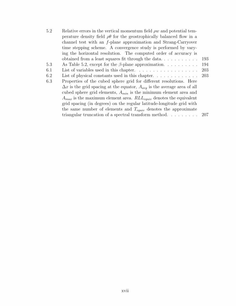
∆x is the grid spacing at the equator, Aavg is the average area of allcubed sphere grid elements, Amin is the minimum element area andAmax is the maximum element area. RLLequiv denotes the equivalentgrid spacing (in degrees) on the regular latitude-longitude grid withthe same number of elements and Tequiv denotes the approximatetriangular truncation of a spectral transform method. . . . . . . . . 103

4.2 Relative errors in the height field h for Williamson et al. (1992) TestCase 1 – advection of a cosine bell (at a resolution of 40 × 40 × 6and after t = 12 days) for the FV3s scheme (top) and FV4 scheme(bottom). . . . . . . . . . . . . . . . . . . . . . . . . . . . . . . . . 131

4.3 Relative errors in the height field h for Williamson et al. (1992) TestCase 2 – Geostrophically balanced flow (at t = 5 days with α = 45)for the FV3s scheme with Rusanov, Roe and AUSM+-up Riemannsolvers. The computed order of accuracy is obtained from a leastsquares fit through the data. . . . . . . . . . . . . . . . . . . . . . . 136

4.4 As Table 4.3 except with the FV4 scheme. . . . . . . . . . . . . . . 1374.5 Relative errors in the height field h for Williamson et al. (1992) Test

Case 3 – Geostrophically balanced flow with compact support (att = 5 days with α = 60) for the FV3s scheme with Rusanov, Roeand AUSM+-up Riemann solvers. The computed order of accuracyis obtained from a least squares fit through the data. . . . . . . . . 141

4.6 As Table 4.5 except with the FV4 scheme. . . . . . . . . . . . . . . 1424.7 The approximate computational performance for each of the numeri-

cal schemes paired with each Riemann solver, as obtained from serialruns on a MacBook Pro with 2.4 GHz Intel Core 2 Duo. The timingscorrespond to the number of seconds required to simulate one day ofWilliamson test case 2 (described in Section 4.7.2) on a 40 × 40 × 6grid. A CFL number of 1.0 is used in all cases. . . . . . . . . . . . . 156

5.1 List of parameters and physical constants used in this chapter. . . . 163

xvi

5.2 Relative errors in the vertical momentum field ρw and potential tem-perature density field ρθ for the geostrophically balanced flow in achannel test with an f -plane approximation and Strang-Carryovertime stepping scheme. A convergence study is performed by vary-ing the horizontal resolution. The computed order of accuracy isobtained from a least squares fit through the data. . . . . . . . . . . 193

5.3 As Table 5.2, except for the β-plane approximation. . . . . . . . . . 1946.1 List of variables used in this chapter. . . . . . . . . . . . . . . . . . 2036.2 List of physical constants used in this chapter. . . . . . . . . . . . . 2036.3 Properties of the cubed sphere grid for different resolutions. Here

∆x is the grid spacing at the equator, Aavg is the average area of allcubed sphere grid elements, Amin is the minimum element area andAmax is the maximum element area. RLLequiv denotes the equivalentgrid spacing (in degrees) on the regular latitude-longitude grid withthe same number of elements and Tequiv denotes the approximatetriangular truncation of a spectral transform method. . . . . . . . . 207

xvii

LIST OF APPENDICES

Appendix

A. Calculation of anti-derivatives . . . . . . . . . . . . . . . . . . . . . . 253

B. High-order bisected element reconstruction . . . . . . . . . . . . . . . 262

C. The gnomonic cubed-sphere projection . . . . . . . . . . . . . . . . . 265

D. The equiangular cubed-sphere projection . . . . . . . . . . . . . . . . 269

E. Treatment of panel boundaries . . . . . . . . . . . . . . . . . . . . . . 272

F. Converting between η and z coordinates . . . . . . . . . . . . . . . . . 275

G. Geometric properties of cubed-sphere coordinates . . . . . . . . . . . . 277

H. The shallow-atmosphere approximation . . . . . . . . . . . . . . . . . 284

xviii

ABSTRACT

Atmospheric Modeling with High-Order Finite-Volume Methods

by

Paul Aaron Ullrich

Chair: Christiane Jablonowski

This thesis demonstrates the versatility of high-order finite-volume methods for

atmospheric general circulation models. In many research areas, these numerical

methods have been shown to be robust and accurate, and further have many proper-

ties which make them desirable for modeling atmospheric dynamics. However, there

have been few attempts to implement high-order methods in atmospheric models, and

none that use finite-volume methods. High-order methods are desirable for future

model development due to their superior wave propagation properties and necessity

when using adaptive mesh refinement.

The thesis describes in detail a hierarchy of atmospheric models that utilize high-

order finite-volume methods. The hierarchy includes a 2D shallow-water model, both

2D and 3D non-hydrostatic models and a 3D non-hydrostatic dynamical core in

spherical geometry. These models span atmospheric motions that range from the

microscale, mesoscale to the global-scale regime while essentially leaving the under-

xix

lying numerical scheme unchanged. A cubed-sphere computational grid has been

chosen for the global models, due to its relative uniformity as compared with the tra-

ditional regular latitude-longitude grid. First, the thesis documents the development

of a finite-volume-based remapping scheme for accurately converting data between

cubed-sphere and latitude-longitude meshes. An analysis of several finite-volume-type

methods in 1D for advection is then presented, with some emphasis on models with

grid adaptation. Furthermore, the thesis describes the formulation of the model hier-

archy that represents a gradual increase in complexity and thereby serves as a testbed.

The 2D (x-y) shallow-water model on the sphere evaluates explicit time-stepping al-

gorithms and demonstrates how to accurately handle the panel boundaries of the

cubed-sphere mesh. The 2D-slice (x-z) and 3D non-hydrostatic finite-volume models

in Cartesian geometry introduce an implicit-explicit time-splitting technique needed

to properly handle the small grid spacings and high-speed waves in the vertical direc-

tion. Finally, a novel 3D non-hydrostatic high-order finite-volume dynamical core in

cubed-sphere geometry is presented. The thesis demonstrates that high-order finite-

volume methods are a viable and promising option for future atmospheric models, and

an important stepping stone for next-generation atmospheric model development.

xx

CHAPTER I

Introduction

1.1 Why do we Build Models?

In 1963, American mathematician and meteorologist Edward Lorenz published

his seminal paper “Deterministic Nonperiodic Flow” (Lorenz , 1963). Lorenz demon-

strated that even a relatively simple system of partial differential equations that arose

from the governing equations of atmospheric motions can lead to chaotic nondeter-

ministic behavior with very strong dependence on the initial conditions. Hence, he

argued, without exacting knowledge of the initial conditions the atmosphere was ef-

fectively unpredictable after even a few days. Lorenz’s work had triggered significant

debate within the atmospheric community that still lingers to today; namely, if pre-

dicting the future behavior of the atmosphere is not only difficult, but effectively

impossible, what is the point in trying to model it?

To some degree, models do not yield explanations analogous to those of rigorous

theory. Yet, models cannot be classified as observational science, which cannot make

future predictions based on incomplete data. In fact, since its inception, the numer-

ical approach has been an altogether different beast. With the advent of modern

numerical methods, modelers could now conduct “experiments” that were previously

inaccessible. If one were interested in how the general circulation of the atmosphere

would change if the Earth had no continents, for example, models could now give

1

answers that could not be found by other methods. Over the past fifty years, atmo-

spheric models have given us incredible insight into the regional and global influences

of the changing climate. However, Lorenz’s words still hold true – atmospheric models

cannot determine the weather next year, but their value is instead found in answering

questions about statistical properties or long term trends of global behavior. As mod-

els more closely match observations of our world, we can be reassured that we have

understood the underlying equations and mechanisms that drive the climate system.

This thesis focuses on the dynamical core component of general circulation models

(GCMs), as depicted in Figure 1.1. The dynamical core is an essential component

of any large-scale model and is responsible for the solution of the fluid equations. It

manages thermodynamic quantities, including density, pressure and temperature as

well as the wind velocity. With the advent of modern supercomputing, massively

parallel computers have become available that can now model the Earth down to

scales of only a few kilometers. Most existing dynamical cores are not well-designed

for computing on these scales and so there is an increasing push for the development

of next-generation software for atmospheric models. This work focused on developing

new technologies, as well as translating existing technologies from other fields, that

would allow us to build a next-generation atmospheric model using methods which

have been proven to be robust, efficient and accurate.

1.2 A Brief History of Numerical Weather Prediction (Be-

fore 1955)

Before proceeding, it is pertinent to review the history of general circulation mod-

els and the developments that have led us to the software system we use today. It

is not our goal to provide a complete history of numerical methods for the atmo-

spheric sciences. For a more complete story, we refer the reader to books such as

2

Figure 1.1:A cross-section of a general circulation model, identifying variables andinteractions which compose the dynamical core (shaded region) and thosewhich are handled by physics (unshaded region).

3

Edwards (2010), Harper (2008) or Randall (2000). An excellent essay by Spencer

Weart on the development of general circulation models for climate is also available

from http://www.aip.org/history/climate/GCM.htm.

The first attempts at predicting the behavior of the atmosphere occurred nearly

a century and a half ago, pioneered by the work of Robert FitzRoy in the 1860s. Us-

ing only telegraph systems to relay local weather information between base stations

across Europe, he produced the first synoptic charts of England and coined the term

“weather forecast.” Into the 1900s advancing technology led to increasingly better

observation data, however, meteorologists of the time still constructed their forecasts

exclusively via historical weather patterns. The idea that the atmosphere could be

treated as a mathematical system was not explored until 1916 when Norwegian me-

teorologist Vilhelm Bjerknes introduced the first set of equations to describe motions

of the atmosphere.

Although Bjerknes’ first work is considered to be the cornerstone in the study

of atmospheric motions, his equations were too complicated to provide insight into

the fundamental dynamics of the atmosphere. In 1922, British mathematician Lewis

Fry Richardson introduced a more complete numerical system for the atmosphere

(Richardson, 1922) and with it a method for performing weather forecasting in a

numerical framework. His idea, modeled after a method mathematicians referred

to as finite-difference solutions, was to break up a given regional domain into a set

of grid cells, each of which stored some component of the state of the atmosphere.

The equations governing the atmosphere could then be discretized and evaluated

to step forward in time. His greatest achievement was in putting this method into

practice, performing months of tedious hand calculations with the goal of predicting

the evolution of a weather system over central Europe over the period of one day.

Sadly, his calculation was also a dramatic failure, as he predicted a huge rise in

pressure (145 mbars) when, in fact, the pressure was more or less static. Although it

4

would not arise until years later, his error was effectively in using an unstable choice

of timestep for his calculations. Under his approach small ampltiude variations in the

pressure field were amplified and led to large-scale disturbances in the solution.

Another shortfall of Richardson’s approach was its complexity. As stated by

Richardson himself, “the scheme is complicated, because the atmosphere itself is

complicated.” Even a one day forecast required thousands of tedious arithmetic cal-

culations. With no concept of modern computing, Richardson’s vision for weather

prediction required tens of thousands of people to simultaneously perform “compu-

tations.” Even then, results would only arrive as fast as weather occurred in reality.

In the mathematics community, work on finite-difference solutions of partial dif-

ferential equations continued. In 1928, Courant, Friedrichs and Lewy published their

fundamental work on stability of numerical methods (Courant et al., 1928). Nonethe-

less, it was not until the advent of modern computing that it became feasible to

perform the computations necessary to predict atmospheric motions.

In the 1940s, John von Neumann had significant success in computing the behav-

ior of explosions using numerical methods. He could see the parallels of his explosion

simulations and numerical weather prediction, and vocally advocated for the use

of modern computers in numerical models of the atmosphere. Jule Gregory Char-

ney, who had come from Carl-Gustaf Rossby’s pioneering meteorology department

at the University of Chicago, was recruited by Von Neumann to develop a numerical

framework for weather prediction. Richardson’s equations were the starting point,

but Charney quickly realized that filtering of these equations was necessary to make

large-scale calculations feasible. The first successful numerical weather prediction ex-

periment finally came about in 1950, performed by Charney at Princeton University

on ENIAC (Charney et al., 1950). Following Richardson’s approach, they divided

the atmosphere over North America into grid cells with a spacing of roughly 700 km.

The time step of these simulations was approximately 3 hours and the calculation

5

was computed purely in 2D. The simulations were far from perfect, but numerically

stable and had enough observed features to motivate continued research.

It did not take long for real-time numerical weather prediction to be adopted

by meteorologists worldwide. The first real-time numerical weather prediction ex-

periments were performed by the Royal Swedish Air Force Weather Service in 1954

(Bergthorsson et al., 1955). In North America, the Weather Bureau established the

Joint Numerical Weather Prediction Unit, which in May of 1955 began issuing real-

time forecasts. Although primitive, these calculations were believed to be reasonably

reliable for up to three days in advance.

Since these early simulations, the infrastructure of predicting the weather has

become a resounding success. With advancing technology and computational power,

it has even become an integral part of our everyday lives.

1.3 The First General Circulation Models (1955-1965)

Up until 1955, weather prediction efforts were limited to regional scales. Ob-

servational data, which were necessary for a model’s initialization, were not reliable

enough to initialize global models so the idea of extending weather forecasting models

to global scales was perceived as unnecessary. Nonetheless, academic efforts began

in 1955 to model the general circulation of the Earth. The first atmospheric general

circulation model was developed by Norman Phillips at Princeton University in 1955

(Phillips , 1956). His computer system held a mere five kilobytes of memory, with an

additional ten kilobytes of data storage. He developed an improved set of equations

for the two-layer atmosphere and modeled circulation on a cylinder 17 cells high and

16 in circumference. The resulting simulation produced a plausible jet stream and a

realistic-looking weather disturbance that evolved in time.

Von Neumann enthusiastically publicized Phillips’ results, which quickly led to

government funding for a long-term project to model the global circulation. In 1955,

6

Joseph Smagorinsky, who at the time worked at the U.S. Weather Bureau, directed

the development of a general circulation model of the entire three-dimensional atmo-

sphere built from the primitive equations (Smagorinsky , 1983). In 1958, Smagorinsky

invited Syukuro Manabe, who had studied at Tokyo University, to join the team. The

contributions of Manabe led to the development of physical parameterizations for ra-

diative transfer, as well as ocean, land and ice exchange processes. It took until 1965

before Manabe’s group had completed, to some degree, a three-dimensional global

model that incorporated nine vertical levels (Manabe and Smagorinsky , 1965). This

model would be the forerunner for the GCMs developed under the banner of the

Geophysical Fluid Dynamics Laboratory (GFDL, Princeton).

Simultaneous with the development of the U.S. Weather Bureau model, another

model was under development at the University of California at Los Angeles (UCLA).

Motivated by Phillips’ 1956 paper, Yale Mintz undertook an ambitious program to

advance the development of GCMs. He recruited Akio Arakawa, also from Tokyo

University, to develop the mathematical foundation for another general circulation

model. By 1964 they had developed a two-layer model that, unlike the Manabe

model, incorporated realistic orography over the entire globe (Mintz , 1965; Arakawa,

1970). Their work ended up being a forerunner for many future modeling groups,

including the Goddard Institute for Space Sciences (GISS) model. Work from both

Mintz and Manabe was later incorporated into the European Centre for Medium-

Range Weather Forecasts (ECMWF) model.

By the end of the 1960s, half a dozen GCMs were already in development, in-

cluding teams at the UK Met Office and the National Maritime Center (NMC) and

a team at the National Center for Atmospheric Research (NCAR), led by Warren

Washington and yet another Tokyo University graduate, Akira Kasahara (Kasa-

hara and Washington, 1967). For a “family tree” of GCM development, we refer

to http://www.aip.org/history/climate/xAGCMtree.htm.

7

1.4 Algorithmic Development (1965-2000)

In 1965 a panel of the U.S. National Academy of Sciences reported on recent devel-

opments in GCMs, observing that global models were largely successful at reproduc-

ing gross features of the atmosphere. Nonetheless, there were significant shortfalls in

these models that could only be addressed by substantially increased computational

power (National Academy of Sciences , 1966). Equally important, however, was the

development of algorithms that produced improved results with fewer computations.

Two problems that were a proverbial thorn in the side of GCM developers were

the poles of the simulation grid. Up until 1965 GCMs had largely used a latitude-

longitude plane for their simulations on the sphere. Although this grid is perhaps the

most natural choice, it is inefficient computationally since it leads to small physical

grid spacing near the poles. A reduced-resolution grid was proposed by Kurihara

(1965), which kept the latitude-longitude mesh but removed grid cells in the lon-

gitudinal direction at high latitudes to maintain grid uniformity. Grids based on

an icosahedral projection were proposed by Sadourny et al. (1968) and Williamson

(1968), and referred to as geodesic grids. A grid based on a cubic projection and

known as a “cubed-sphere grid” was later developed by Sadourny (1972). These

grids were an elegant solution to the pole problem, but in many cases were not com-

petitive with existing models. As a consequence, uniform grids were largely not used

in operational atmospheric models until the mid-1990s. One notable exception was

the GFDL SKYHI model (Fels et al., 1980), which used a reduced resolution grid

throughout the 1980s.

In the 1970s other innovations aimed at the finite-difference methods that had been

used in most GCMs. Instead of dividing the planet’s surface into a grid of elements,

the equations of motion were rewritten in terms of spherical harmonics. This “spectral

transform” technique simplified many computations and allowed the pole problem to

be sidestepped entirely, but was only feasible with faster computers. Nonetheless,

8

the spectral transform method was very popular in the GCM community and is even

in use in models today. For example, the ECMWF model still uses the spectral

transform method for forecasts, having adopted it into their forecasting systems in

1983. However, the spectral transform method is not without its disadvantages.

Firstly, monotonicity and positivity are not guaranteed – that is, numerical errors can

result in significant spurious overshoots and undershoots in flow variables, which may

result in negative tracer concentrations. Secondly, dispersive errors in the spectral

model can lead to “Gibbs ringing” in regions where solutions are not perfectly smooth,

and so high-frequency waves must be explicitly damped. Finally, spectral transform

methods require the use of global Fourier transforms, which reduces the efficiency

of these models on parallel computational architectures. Nonetheless, the spectral

transform method proved to be a very effective technique for global atmospheric

models.

By the mid-1980s, substantial progress had been made in other research areas that

were also tied to hydrodynamics. Aerospace and astrophysics, in particular, had de-

veloped their own algorithmic treatments of the fluid equations, although their work

often dealt with very-high-speed flows. Interestingly, much of this work was again due

to the involvement of John von Neumann, who had driven interest in numerical meth-

ods for atmospheric phenomena. Finite-volume methods had become very popular in

these fields, but were largely unheard of in the atmospheric sciences. Finite-volume

methods had their own fundamental history, tracing their roots back to the work of

Godunov (1959), who had developed conservative finite-volume methods for modeling

shockwaves, and subsequently was involved in developing a class of methods which

are today referred to as Godunov-type methods. This work was later extended by

Bram van Leer in a series of papers (van Leer , 1974, 1977, 1979) which described

an approach for extending Godunov’s method to second-order accuracy. This work

was simultaneous with that of Boris and Book (1973), who developed flux-corrected-

9

transport (FCT) methods (extended by Zalesak , 1979). Later, Colella and Woodward

(1984) developed the piecewise-parabolic method (PPM) for gas hydrodynamics prob-

lems, which was a Godunov-type finite-volume method of third-order accuracy. Other

prominent figures in computational fluid dynamics research at this time included Pe-

ter Lax (Lax and Wendroff , 1960), Robert MacCormack (MacCormack , 2003), Philip

Roe (Roe, 1981), Amiram Harten (Harten et al., 1983) and Stanley Osher (Osher and

Sethian, 1988).

In 1987, Richard Rood wrote a fundamental paper comparing many numerical

methods for advection (Rood , 1987). Advection had been a significant problem in at-

mospheric models, since it required monotonicity preserving filters and was generally

poorly handled by spectral transform methods. His work drew heavily on research

from other fields, which generally had only minimal contact with the atmospheric

sciences. In particular, he advocated for finite-volume methods, which preserved

positive-definite results, guaranteed conservation of mass and maintained high accu-

racy. This work contributed prominently to the development of a finite-volume dy-

namical core with Shian-Jiann “S.J.” Lin (Lin and Rood , 1996; Lin and Rood , 1997;

Lin, 2004) at NASA, which used a staggered grid and a piecewise-parabolic-type re-

construction procedure. This dynamical core is perhaps one of the most well-known

dynamics models today, and remains well-used within GFDL, NASA’s Goddard Earth

Observing System Model, Version 5 (GEOS-5) and NCAR’s Community Atmosphere

Model (CAM).

1.5 The Modern State of Numerical Methods for Atmospheric

Models (2000-Today)

By the end of the 20th century, computational power was continuing to increase

exponentially. The advent of supercomputing had led to massively parallel systems,

10

which consisted of thousands or more interconnected processors. Models running on

these systems can now reach resolutions on the order of 10 kilometers or less – far

beyond anything Richardson could have dreamt of! However, it was also clear that

many of the operational GCMs were not well-designed to truly harness these sys-

tems. Communication between processors was beginning to be a bottleneck, since

many prominent numerical methods (spectral transform methods, as well as finite-

difference or finite-volume methods which are built on a latitude-longitude grid) re-

quire a substantial amount of communication between processors at each timestep.

Dozens of atmospheric models are in use today, with applications ranging from

experimental science to operational forecasting. Recent developments in modeling

atmospheric dynamics have tended away from the latitude-longitude grid, instead

returning to uniform grids, including the icosahedral or cubed-sphere grids. This

choice has allowed for the design of models which can be run at very fine resolutions

on vast parallel computing systems. The drive towards finer and finer resolutions

has also forced many models to re-evaluate the basic equations that governs their

dynamics. At scales less than ten kilometers the hydrostatic approximation is no

longer valid, and so models typically resort to using the full non-hydrostatic primitive

equations. A list of many models that are either under development or operational is

given below.

1.5.1 Hydrostatic Models

Hydrostatic models approximate the vertical structure of the atmosphere to be in

a state of hydrostatic balance. Under this approximation, the vertical velocity is no

longer a prognostic quantity but is instead determined using the computed pressure

and divergence of the horizontal velocity field. This approximation works well when

the horizontal grid spacing is much larger than the vertical grid spacing, and so has

been a mainstay of atmospheric models for the past several decades.

11

• CAM Eulerian model: (NCAR, Boulder, Colorado) (Collins et al., 2004)

A hydrostatic model that uses the spectral transform method with triangular

truncation on a Gaussian grid with hybrid η vertical coordinate (Simmons and

Burridge, 1981).

• CAM/GEOS finite-volume model: (NCAR, Boulder, Colorado and NASA

Goddard Space Flight Center, Greenbelt, Maryland) (Lin and Rood , 1996; Lin,

2004) A hydrostatic model that uses a monotonic and potentially third-order

piecewise-parabolic finite-volume reconstruction (overall second-order in space

due to flux evaluation) on a latitude-longitude grid, mixed Arakawa D/C-grid

staggering and floating Lagrangian vertical coordinate. A polar filter is em-

ployed to remove grid-scale noise in the polar regions.

• CSU model: (Colorado State University, Fort Collins, Colorado) (Ringler

et al., 2000) A third-order finite-differences based model with icosahedral hexag-

onal grid.

• NASA/GFDL finite-volume cubed-sphere model: (NASA Goddard Space

Flight Center, Greenbelt, Maryland / Geophysical Fluid Dynamics Laboratory,

Princeton, New Jersey) (Putman and Lin, 2007; Putman and Lin, 2009) As

CAM/GEOS finite-volume model except on a cubed-sphere grid, removing the

need for polar filtering.

• NOAA Flow-following finite-volume Icosahedral Model (FIM): (Lee

et al., 2006; Henderson et al., 2010) A second-order finite-volume model on the

icosahedral grid using flux-corrected transport with semi-Lagrangian vertical

levels.

• German Weather Service GME model: (Majewski , 1998; Majewski et al.,

2002) A hydrostatic model that uses second-order finite-differences on an icosa-

12

hedral grid with unstaggered variables and hybrid η vertical coordinate.

• GISS ModelE: (NASA Goddard Institute for Space Studies, New York, NY)

(Schmidt et al., 2006) A hydrostatic model that uses second-order centered

finite-differences plus the quadratic upstream method of Prather (1986) (semi-

Lagrangian discontinuous Galerkin) for advection. The model is built on a

latitude-longitude grid with B-grid staggering and hybrid η vertical coordinate.

• High-Order Method Modeling Environment (HOMME) models: (NCAR,

Boulder, Colorado) (the Spectral Element Atmosphere Model, SEAM) (Fournier

et al., 2004; Taylor et al., 2008) A set of hydrostatic models built on finite-

element-type compact methods, including spectral element and discontinuous

Galerkin in the horizontal and second-order finite-differences with hybrid η co-

ordinate in the vertical.

1.5.2 Non-hydrostatic Models

Non-hydrostatic models make no approximation to the vertical structure of the

atmosphere and so allow for features such as horizontal transport of vertical momen-

tum.

• Icosahedral Non-hydrostatic (ICON) GCM: (Max-Planck Institute for

Meteorology, Hamburg, Germany and DWD) (Wan, 2009; Gaßmann, 2010)

Initially, ICON was developed as a hydrostatic prototype model, but has re-

cently been updated to use the full non-hydrostatic equations. This model uses

a finite-difference method on an icosahedral grid with Arakawa C-grid stagger-

ing and hybrid η vertical coordinate.

• ECMWF Integrated Forecast System (IFS) model: (Wedi et al., 2010) A

non-hydrostatic model using the spectral transform method with semi-Lagrangian

transport and built on the reduced latitude-longitude grid. Note that IFS was

13

developed as a hydrostatic model and has been in operational use for decades.

Recently, it was extended to a non-hydrostatic version that is currently under-

going testing.

• Global Environmental Multiscale (GEM) model: (Yeh et al., 2002) An

implicit second-order semi-Lagrangian model using an Arakawa C-grid and

hydrostatic-pressure based vertical coordinate, and built on a latitude-longitude

grid.

• MIT GCM: (Massachusetts Institute of Technology, Boston, Massachusetts)

(Adcroft et al., 2004) A finite-volume cubed-sphere-grid model with height-based

vertical coordinate and shaved-cell topography.

• Model for Prediction Across Scales (MPAS): (Skamarock et al., 2010)

(NCAR, LANL/DOE) A new non-hydrostatic global model designed to su-

percede the Weather Research and Forecasting (WRF) model. Uses conserva-

tive 2nd-order finite-differences on a icosahedral hexagonal mesh with Arakawa

C-grid staggering, height-based vertical coordinate and 3rd-order split-explicit

Runge-Kutta time integration.

• Non-hydrostatic ICosahedral Atmospheric Model (NICAM): (Tomita

and Satoh, 2004) Developed in cooperation with the Center for Climate Sys-

tem Research (CCSR, Japan). This non-hydrostatic atmospheric model uses

2nd-order finite-differences on an icosahedral grid with horizontally unstaggered

variables and vertically staggered vertical velocity. The vertical coordinate is

height-based.

• Non-hydrostatic Icosahedral Model (NIM): (Govett et al., 2010) (Earth

System Research Laboratory, NOAA) A Riemann-solver-based finite-volume

model on an icosahedral hexagonal grid with monotonic Adams-Bashforth third-

14

order multistep time integrator and height-based vertical coordinate.

• Ocean-Land-Atmosphere Model (OLAM): (Walko and Avissar , 2008)

(Duke University) A non-hydrostatic, finite-volume based model using an icosa-

hedral grid with Arakawa C-grid staggering, height-based vertical coordinate

and shaved cells for representing topography.

• UK Met Office Unified Model: (Davies et al., 2005; Staniforth and Wood ,

2008) A non-hydrostatic model using a conservative finite-difference approach

on a latitude-longitude grid with height-based vertical coordinate. Both the

shallow and deep-atmosphere equations as well as the hydrostatic and non-

hydrostatic equations are supported in this model.

1.6 Future Trends in Model Development

Looking forward, it is clear that substantial work remains to be done in developing

next-generation general circulation models. Scalability on massively parallel systems

is an essential requirement of any future model, and so should be a cornerstone of any

future designs. Further, new technologies will play an increasingly important role,

such as graphical processing units (GPUs), which have the potential to dramatically

speed up existing simulations.

1.6.1 The Cubed-Sphere Grid

As mentioned previously, the icosahedral (geodesic) grid has many desirable prop-

erties, but since it relies on either triangles or hexagons (and pentagons) to form each

grid cell, it is more difficult to optimize organization of computational grid cells than

on a more structured grid. In 1996, the cubed-sphere grid was revived by Ronchi et al.

(1996) and later used as the basis for a shallow-water model by Rancic et al. (1996).

Since then, shallow-water models have been developed using the cubed-sphere that

15

utilize finite-volume methods (Rossmanith, 2006; Ullrich et al., 2010), multi-moment

finite-volume (Chen and Xiao, 2008), the discontinuous Galerkin method (Nair et al.,

2005) and the spectral element method (Taylor et al., 1997). The spectral element

method was successfully extended to a full hydrostatic atmospheric model (the Spec-

tral Element Atmosphere Model, SEAM) (Fournier et al., 2004), which is part of the

High-Order Method Modeling Environment (HOMME). HOMME incorporates both

the spectral element and discontinuous Galerkin methods, and has proven to scale

efficiently to hundreds of thousands of processors. More recently, the GFDL finite-

volume dynamical core has been modified to utilize a cubed-sphere grid (Putman and

Lin, 2009; Putman and Suarez , 2009), and has been demonstrated to also be very

effective at high resolutions.

1.6.2 Adaptive Mesh Refinement

Although computational power has increased substantially in recent years, large

parallel systems are still required to properly resolve many important atmospheric

features. In order to reduce the computational burden of these fine-scale simulations,

the next generation of atmospheric models will likely need to rely on adaptive mesh

refinement (AMR). Mesh refinement refers to the addition of grid elements to regions

with small-scale features so as to reduce errors that arise due to insufficient resolution.

Static mesh refinement implies that the grid does not change in time, but regions of

significant dynamical behavior, such as the equator, are initially enhanced. Dynamic

mesh refinement is similar, but allows the grid to change over the process of the

simulation.

Mesh refinement can be categorized into either using conformal or non-conformal

grids. Conformal grids use a smooth mapping between some initial regular mesh (such

as a Cartesian or hexagonal grid) and the desired mesh. These grids include stretched

grids, wherein grid elements are slowly distorted so as to enhance resolution in certain

16

locations (Fox-Rabinovitz et al., 1997, 2006). Non-conformal grids, on the other hand,

are not the product of such a conformal mapping. Block adaptive grids, for instance,

are an example of a non-conformal grid (Berger and Oliger , 1984; Berger and Colella,

1989; Skamarock et al., 1989; St-Cyr et al., 2008). Non-conformal meshes are largely

preferred for dynamical mesh refinement since they only require local modification of

the mesh when additional resolution is added or removed.

Grid reflection is a prominent issue with non-conformal meshes that will be dis-

cussed in this thesis. When a wave packet propagates through a resolution discon-

tinuity, the discontinuous modification of the dispersion relation leads to behavior

analogous to what one would expect at a discontinuity in the physical properties of

the fluid. As a consequence, part of the wave is transmitted and the remainder re-

flected. The artificial reflection of the wave packet can lead to the phenomenon of

trapped waves in regions of fine grid resolution, which can in turn affect the accuracy

of the solution.

1.7 Outline of Thesis

In this thesis we present our ongoing work on high-order finite-volume methods in

the context of atmospheric GCMs. In many research areas, these methods have been

demonstrated to be robust and accurate, and further have many properties which

make them desirable for modeling atmospheric dynamics.

This thesis is organized as follows. In Chapter 2 we introduce the cubed-sphere ge-

ometry in the context of the Geometrically Exact Conservative Remapping (GECoRe)

scheme, which was developed for conservative remapping between the cubed-sphere

and latitude-longitude grid. Chapter 3 pursues a theoretical analysis of the proper-

ties of various high-order finite-volume methods, particularly in the context of refined

grids. In Chapter 4 we develop a high-order finite-volume shallow water model on

the cubed-sphere and compare several methods for computing element fluxes using

17

Riemann solvers. The problem of horizontal-vertical aspect ratio in non-hydrostatic

atmospheric models in Cartesian geometry is tackled in Chapter 5, wherein we propose

an implicit-explicit Runge-Kutta-Rosenbrock (RKR) approach for coupling horizontal

and vertical motions while maintaining high-order-accuracy and a timestep limit that

is only proportional to the horizontal grid spacing. In Chapter 6 we discuss an exten-

sion of the high-order finite-volume shallow-water model on the cubed-sphere grid to

a fully non-hydrostatic shallow-atmosphere model utilizing the implicit-explicit split-

ting approach. Finally, conclusions and future work are presented in Chapter 7. A

substantial portion of the mathematics behind the cubed-sphere grid and high-order

finite-volume methods can be found in the Appendices.

18

CHAPTER II

Geometrically Exact Conservative Remapping

2.1 Introduction

Land, ocean and atmosphere components of coupled climate system models are

often implemented on different spherical grids, individually designed to enhance the

accuracy or capture features unique to their respective settings. Historically, the

regular latitude-longitude (RLL; see Table 2.1 for a complete list of acronyms used

in this chapter) grid has been the predominant choice for global atmospheric models,

but problems associated with the polar singularity persist, and hence this grid is not

well-suited for highly scalable atmospheric models. Much interest in recent years

has been instead directed towards the development of atmospheric solvers defined on

more isotropic spherical grids. For example, the cubed-sphere grid, which divides

the polar singularities among eight weaker singularities located at the corners of a

cube, and is otherwise highly scalable on parallel architectures. The cubed-sphere

grid was originally introduced by Sadourny (1972), and more recently reintroduced

by Ronchi et al. (1996) and Rancic et al. (1996) with equiangular grid spacing and

orthogonality. For the land component, however, the RLL grid does not pose polar

singularity problems as is the case for the atmosphere (with the current complexity

of land models). Neither does the land model seem to be susceptible to scalability

problems since most of the computation is in vertical columns rather than in the

19

Table 2.1: List of acronyms used in this chapter.

Acronym

GECoRe Geometrically Exact Conservative Remapping()-M suffix stands for Monotone filter appliedPCoM Piecewise Constant methodPLM Piecewise Linear methodPPM Piecewise Parabolic MethodRLL Regular Latitude-LongitudeABP Alpha-Beta-Panel (Equiangular cubed-sphere Coordinates)SCRIP Spherical Coordinate Remapping and Interpolation PackageCaRS Cascade Remapping between Spherical grids

horizontal. Hence for the foreseeable future the RLL grid seems to be a viable and

convenient grid for land model components.

An intricate problem introduced by defining the model components on different

spherical grids is that the exchange of information between the grids is non-trivial and

requires a regridding algorithm. In a coupled climate system model it is paramount

that the regridding process is not a spurious source or sink for first-order moment

variables such as mass. To prevent the generation of unphysical negative and/or

large values, the regridding must also be shape-preserving/monotone for mixing-ratio

related variables. Regridding with these constraints, conservation and monotonicity,

is a non-trivial problem if higher than first-order accuracy is desired.

The regridding problem is not only limited to a static grid-to-grid information

transfer setting. The problem is essentially the same for finite-volume advection

schemes where the mass-transport into a given cell is given in terms of integrals

over overlapping areas. In fact, methods developed for advection schemes can be

readily applied in grid-to-grid regridding problems such as articulated by Margolin

and Shashkov (2003). A major difference between the advection regridding problem

and static grid-to-grid regridding is that the source or target grid is not static for

advection problems. Hence the regridding algorithm must be able to deal with a

20

large class of source or target grids changing dynamically at each time step. For grid-

to-grid regridding the problem is static, facilitating certain parts of the algorithm.

For example, the regridding problem can be optimized for specific grid pairs. On the

other hand, the advection problem is usually constrained by Courant numbers and

the number of source and target grid cells are identical which constrains the overlap

regions. On the contrary, grid-to-grid regridding does not have that constraint so

many source grid cells can overlap a particular target grid cell and vice versa.

A strategy for doing conservative regridding without ad hoc conservation fixers is

to reconstruct a sub-grid-cell distribution in each source grid cell with conservation as

a constraint and then integrate the sub-grid-cell distributions for the respective source

grid cells over the overlap areas. This process of conservative transfer of variables

between grids is referred to as remapping or rezoning. Depending on the source and

target grid cell geometries the overlap regions over which one must integrate can be

very complex. Hence direct integration on the sphere of the overlap areas seems like

an almost impossible task in terms of algorithmic complexity. Note, however, that it

has been done in Cartesian geometry in the context of advection (see Rancic 1992).

The problem can be greatly simplified by making use of the powerful mathematical

theorem, Gauss’s divergence theorem, that converts area integrals into line integrals

(see Dukowicz and Kodis 1987). This is the approach taken in the most widely

used regridding software in the climate community called the Spherical Coordinate

Remapping and Interpolation Package (SCRIP, Jones 1999). Also in the algorithm

presented in this chapter we make use of Gauss’s divergence theorem.

In order to perform the line integrals on the sphere one usually makes simplifying

assumptions about the cell sides. For example, the sides of the grid cells are approx-

imated by straight lines in (λ, θ)-space in SCRIP. This obviously leads to exact cell

wall representations for the RLL grid but other spherical grids such as the cubed-

sphere grids do not share that property (see Figure 2.1). The remapping algorithm’s

21

Figure 2.1:The cell boundaries of the cubed-sphere south polar panel plotted inCartesian coordinates. SCRIP approximates cell edges by connecting thecell vertices (filled circles) with straight lines in RLL coordinates (dottedlines). The solid lines are the exact ABP cell walls that are great circlearcs.

22

inability to represent the cell sides exactly is here referred to as the geometric error

(Lauritzen and Nair 2007; hereafter referred to as LN2007). In other words, the ge-

ometric error is the deviation from exact closed-form integration along the cell walls.

Unfortunately, exact closed-form integration is not always achievable, except for a

small set of source and target grids. As a consequence, generic conservative remap-

ping schemes, such as SCRIP and CaRS, must apply potentially crude geometrical

approximations in order to yield a conservative and computationally efficient scheme

(Figure 2.1). Perhaps serendipitously, we find that complete removal of geometric

error via exact closed-form integration is possible for the RLL grid and gnomonic

cubed-sphere grids, and hence these grids immediately lend to the development of a

geometrically exact conservative scheme.

Assuming small geometric error, the order of the remapping algorithm is deter-

mined by the accuracy of the sub-grid cell reconstruction. The errors introduced

by the reconstruction are referred to as the derivative error. The simplest recon-

struction is a piecewise constant (first-order) representation in each source grid cell.

This method is inherently monotone but is excessively damping at least in idealized

remapping problems. First-order reconstructions are, for example, used in NCAR’s

Coupled Climate System Model (CCSM3, Collins et al. 2006) through SCRIP for

remapping variables requiring conservation. The effect on climate by using higher-

order remapping in a coupled climate system model is unknown (as far as the authors

are aware) but it seems instinctive to speculate that it could have a significant effect;

especially in areas where remapping is done from a coarse to a fine grid.

Unfortunately, high-order reconstructions are not inherently monotone, making it

harder to achieve conservation, monotonicity and high-order accuracy simultaneously.

LN2007 choose to apply the cascade remapping approach to achieve monotonocity

with high-order reconstructions. This algorithm is referred to as CaRS (monotone

and conservative cascade remapping between spherical grids). In CaRS the remapping

23

problem is split into two one-dimensional problems and hence only one-dimensional

limiters are needed to guarantee monotonicity, making it relatively easy to impose

shape-preservation simultaneously with higher-order reconstructions. Unfortunately,

the CaRS method is inherently prone to geometric errors, although it seems to com-

pensate for these via the higher-order reconstructions that are easily and efficiently

applied in one dimension. The geometric errors can be reduced by artificially in-

creasing the resolution in areas of higher geometric error (see LN2007 for details).

A necessary, but insufficent, condition for completely eliminating the geometric er-

ror is to approximate the grid cells in a two-dimensional manner rather than the

dimensional split approach such as done in CaRS. However, a fully two-dimensional

approach requires fully two-dimensional integrals, reconstructions and limiters. This

greatly increases the complexity of the problem, especially when aiming for higher-

order remapping. SCRIP has the option of performing second-order remapping if the

user supplies the gradient in latitude-longitude coordinates. In theory SCRIP could

be extended to higher-order by including the curvature and high-order derivatives in

the line-integral computations but that route was not explored by Jones (1999) and

is not a trivial extension.

In this chapter we present a new conservative remapping method between gnomonic

cubed-sphere grids and the RLL grids hereafter referred to as GECoRe (geometrically

exact conservative remapping). GECoRe uses Gauss’s divergence theorem to convert

area integrals into line integrals. The line integrals are exact (to machine precision)

for given polynomial sub-grid-cell reconstructions since the lines along which the line

integrals are computed exactly coincide with grid lines on the cubed-sphere and RLL

grid. Consequently the geometric error is completely eliminated in GECoRe. We also

use up to third-order-accurate reconstructions and apply limiters to obtain monotonic-

ity thereby obtaining high-order accuracy and shape-preservation simultaneously in

two dimensions.

24

The paper is organized as follows. In Section 2 we introduce the mathematical

basis for GECoRe, that is, how to compute the potentials needed to convert area in-

tegrals into line integrals, how line integrals are computed exactly and how the fully

two-dimensional reconstructions are approximated. Section 3 covers some practical

considerations such as finding intersections between line segments of the two grids.

The accuracy of GECoRe is assessed in Section 4 by comparing standard error mea-

sures for remapping analytical functions with GECoRe, SCRIP and CaRS between

equi-angular cubed-sphere and RLL grids with different resolutions. A summary is

given in Section 5.

2.2 Geometrically exact conservative remapping

In the context of finite volume methods, we are given the cell-averaged value of a

scalar field for each cell in the source grid, denoted by fn. The remapping problem

then reduces to finding corresponding cell-averaged values in the target grid, denoted

fk, that accurately represent the underlying scalar field. Throughout this chapter we

will use the subscript n to denote a quantity corresponding to a cell of the source grid

and the subscript k to denote a quantity corresponding to a cell of the target grid.

2.2.1 Source and target grids

Of the numerous choices for the cubed-sphere, we will focus on the equiangular

cubed-sphere, where a sphere is decomposed into six identical regions (panels or faces)

and the grid lines on each panel are defined by equispaced central angles (see Fig.

2.2). Hereafter, we will refer to the equiangular cubed-sphere as the ABP (alpha, beta,

panel) coordinate system, in reference to coordinates on the sphere being identified by

the three-element vector (α, β, np), where (α, β) ∈ [−π/4, π/4] are the coordinates on

each panel and np ∈ 1, 2, 3, 4, 5, 6 is the panel index. A mathematical description

of the properties of the equiangular cubed-sphere is given in appendix D.

25

Although we focus on the equiangular projection, we should emphasize that the

GECoRe method is trivially extended to any cubed-sphere grid which is composed

of grid lines parallel to the panel edges, i.e. gnomonic cubed-sphere grids. Notably,

conformal or spring-dynamics grids, where grid lines are “warped” near the corners,

do not fall into this category (see, for example, Putman and Lin (2007) for a review

of several types of cubed-sphere grids). Grids with grid lines that are not parallel to

panel sides can also be captured via this scheme by replacing the exact line-integral

formulas with Gaussian quadrature approximations to the integrals in gnomonic co-

ordinates. Such an approach is taken in the tracer transport scheme described in

Lauritzen et al. (2008). Of course, the geometric error will not be completely elimi-

nated if the cell sides are not great spherical arcs. Note that in such a situation the

geometric error could be reduced by approximating the cell sides by several great-

spherical arc segments.

We will also use Gnomonic coordinates interchangeably with equiangular coordi-

nates. Gnomonic coordinates (x, y) are defined in terms of equiangular coordinates

via

x = a tanα, y = a tan β, (α, β) ∈[−π

4, π

4

]2, (2.1)

where a is a constant denoting the edge length of a concentric cube, which, without

loss of generality we will take to be equal to unity. The Gnomonic projection is impor-

tant for our analysis since any straight line in the Gnomonic projection corresponds

to a spherical arc on the surface of the sphere. A mathematical description of the

properties of the Gnomonic cubed-sphere is given in appendix C.

26

4

6

1

5

2 3

Figure 2.2:An illustration of the regular latitude-longitude (RLL) grid (thin solidlines) and cubed-sphere grid (dotted lines). Thick lines mark the bound-aries of each panel, distinguished by the panel index given in the upper-right corner. By convention we choose for the southern and northernpolar panels to have indices 5 and 6, respectively.

27

2.2.2 Overview of the method

Typically, a conservative remapping scheme is one that satisfies the global conser-

vation condition, ∫A

ftargetdA =

∫A

fsourcedA, (2.2)

where ftarget and fsource are the global scalar field on the target grid and source grid,

respectively. Here the integral is taken over the entire grid surface A (in our case, the

surface of a sphere). The stricter local conservation condition states that for every

cell k on the target grid, the scalar field must satisfy

fk =1

Ak

∫Ak

fdA, (2.3)

where fk denotes the area-averaged scalar field, f the global piecewise reconstruction

on the source grid and Ak the area of cell k. Note that the local conservation condition

can be trivially demonstrated to be a sufficient condition for the global conservation

condition. Now, if cell k in the target grid overlaps N cells in the source grid, one

can write (2.3) as

fk =1

Ak

N∑n=1

∫Ank

fndA, (2.4)

(see Jones 1999 equation (3)) where Ank is the area of the source grid cell n that is

overlapped by the destination cell k, and fn is the local value of the scalar field in

grid cell n (see Fig. 2.3). That is, the averaged value in the destination cell is equal

to the area-normalized contribution from all overlapping cells on the source grid.

A GECoRe type remapping scheme can generally be obtained at any order, with

the order of the method generally depending on the order of the sub-grid scale recon-

struction within each source volume. In general, for a remapping scheme of order h,

28

An

Ak

Ank

Figure 2.3:An example of a quadrilateral target grid cell Ak that overlaps severalsource grid cells. The region overlapped by both Ak and An is denotedby Ank.

the sub-grid scale reconstruction takes the form

fn(x, y) =∑p+q<h

a(p,q)n (x− x0)p(y − y0)q, (2.5)

where the reconstruction coefficients a(p,q)n are constants and x0 and y0 denote the x

and y components of the source-grid cell centroids, defined by

x0 =1

An

∫An

xdA, y0 =1

An

∫An

ydA. (2.6)

In practice, these quantities are computed by transforming the area integrals to line

integrals via Gauss’s divergence theorem (as discussed later). In order to obtain the

desired order of accuracy of the method, the reconstruction coefficients must also be

obtained via a suitably accurate method. The reconstruction (2.5) must also yield

the cell-averaged value of the source volume when integrated over the entire source

volume, i.e.

fn =∑p+q<h

a(p,q)n

1

An

∫An

(x− x0)p(y − y0)qdA. (2.7)

In appendix A we present reasonable choices of the reconstruction coefficients that

29

lead to first-, second- and third-order methods.

The conservative remapping scheme that follows from (2.4) and (2.5) can then be

written as

fk =N∑n=1

∑p+q<h

a(p,q)n w

(p,q)nk , (2.8)

where, following Jones (1999), we have defined the mesh-dependent weights via

w(p,q)nk =

1

Ak

∫Ank

(x− x0)p(y − y0)qdA. (2.9)

The form (2.8) is particularly meaningful, as it emphasizes the separation of the purely

reconstruction-dependent coefficients a(p,q)n and the purely mesh-dependent sub-cell

weights w(p,q)n .

Following Dukowicz and Kodis (1987), we compute the weights (2.9) by converting

them into line integrals using the divergence theorem. Consider an arbitrary vector

field Ψ defined in terms of ABP unit basis vectors (eα, eβ) as Ψ = Ψαeα + Ψβeβ. In

general 2D curvilinear coordinates the divergence is given by

∇ ·Ψ =1√g

[∂

∂x1(√g Ψ1) +

∂

∂x2(√g Ψ2)

], (2.10)

where Ψ1 and Ψ2 are the contravariant components of the vector Ψ and g is the

determinant of the metric. Hence, specifically for cubed-sphere (see (D.8) and (D.9))

we have

∇ ·Ψ = (ρ3 cos2 α cos2 β)

[∂

∂α

(Ψα

ρ cos β

)+

∂

∂β

(Ψβ

ρ cosα

)], (2.11)

where

ρ =√

1 + tan2 α + tan2 β. (2.12)

After integrating (2.11) over the sub-cell Ank and assuming sufficiently smooth bound-

30

aries, we can write the resulting expression in the form

∫Ank

∇ ·Ψ dV =

β2∫β1

α2(β)∫α1(β)

∂

∂α

(Ψα

ρ cos β

)dα dβ +

α2∫α1

β2(α)∫β1(α)

∂

∂β

(Ψβ

ρ cosα

)dβ dα, (2.13)

where α1, α2, β1(α) and β2(α) represent the boundaries of the domain of integration.

Then, on applying the fundamental theorem of calculus, we obtain the divergence

theorem for cubed-sphere coordinates,

∫Ank

∇ ·ΨdV = −∮

∂Ank

[Ψα

ρ cos βdβ +

Ψβ

ρ cosαdα

], (2.14)

where the contour integral is taken in the counter-clockwise direction around the

boundary of a given overlapping volume Ank, here denoted by ∂Ank. Note that the

Jacobian term obtained by expanding the area integral (2.13) cancels with the√g

from the divergence (2.10) and so does not appear in the final form of the contour

integral. The spatial curvature instead comes into play when solving for Ψ via (2.10).

In order to apply the divergence theorem to compute the weights associated with

each line segment over an integrable scalar field φ(α, β, np), we must first obtain a

potential Ψ associated with that field – namely, one that satisfies

∇ ·Ψ = φ. (2.15)

Note that for a given φ, there does not exist a unique potential Ψ, but a family

of potentials Ψ that satisfy (2.15). However, one can obtain a unique potential on

imposing Ψα = 0 and choosing any constant of integration for the potential to equal

zero. This limitation is largely by convention, as we could also choose Ψβ = 0, for

example. However, we find that integration on the RLL grid is generally easier upon

imposing the former constraint, and so we will henceforth apply Ψα = 0 when deriving

31

each potential. Further, we restrict our attention to solving integrals of the form (2.9)

– noting that the integrand of (2.9) can be expanded as terms of the form xpyq (using

(2.1)) – and so use the notation Ψ(p,q) to denote the potential associated with the

scalar field tanp α tanq β. That is, we use (2.11) to define Ψ(p,q) via the differential

equation

∂

∂β

(Ψ

(p,q)β

ρ cosα

)=

tanp α tanq β

ρ3 cos2 α cos2 β, with Ψ(p,q)

α = 0. (2.16)

Note that one may solve (2.16) in terms of either equiangular or Gnomonic coordi-

nates, which are connected via the relation (2.1). In either case we will obtain an

identical expression for the potential.

Since our search algorithm will provide a list of line segments, rather than a list

of contours, a computational implementation of (2.14) will take the form

∫Ank

tanp α tanq βdA = −∑s

I(p,q)s

∣∣(∂Ank)s

, (2.17)

where the summation is taken over all line segments s along the boundary of sub-cell

Ank. Here, I(p,q)s is shorthand notation for the antiderivative over the potential field

obtained from (2.16),

I(p,q)s =

∫Ψ

(p,q)β

ρ cosαdα, (2.18)

and hence it is evaluated at the endpoints of each line segment. A detailed presen-

tation of the calculations and implementation details required for the first-, second-

and third-order accurate schemes are given in appendix A.

2.2.3 Summary of the GECoRe Algorithm

A GECoRe remapping scheme is initialized as follows:

1. Perform a search on the source and target grids, classifying line segments by

type (i.e. constant α, constant β, constant latitude or constant longitude) and

32

keeping track of their endpoints and orientation. Each line segment should then

be associated with at most one ABP cell and one RLL cell.

2. Using (2.9) calculate the weights w(p,q)nk associated with each line segment over

the fields tanp α tanq β, for p + q < h, where h is the order of the method

(this leads to 12h(h + 1) weights per line segment). The weights of each line

segment are computed by simply evaluating the associated antiderivative I(p,q)s

at each endpoint (see Appendix A). Note that one can save memory and online

computation time by instead storing the sum of all weights for a given overlap

cell rather than the weights for individual line segments.

Once the GECoRe scheme is initialized for a particular mesh pair, the resulting

initialization data can be saved to a file for later use. The actual remapping is then

performed as follows:

1. Calculate the reconstruction coefficients a(p,q)s associated with the scalar field,

potentially using neighbouring cell values.

2. Use the weights w(p,q)nk computed in the initialization step, along with (2.8) to

compute the remapped field in each of the target grid cells.

2.3 Practical considerations

In this section we present issues relating to the implementation of the GECoRe

scheme.

2.3.1 Search algorithm

Since we are restricted to RLL and cubed-sphere grids, the search algorithm for

finding line segments is dramatically simplified when compared to the SCRIP algo-

rithm. In fact, this knowledge of the coordinate systems allows us to exactly calculate

33

the line segment endpoints up to machine precision. The proposed technique involves

first searching along longitude and latitude lines to compute intersection points, bin-

ning each line accordingly depending on its corresponding ABP cell. Then a search

within each cell can be performed to obtain all lines of constant α and β within a RLL

cell. This binning procedure results in memory locality of line segments associated

with a given RLL cell, and hence is optimal for remappings from the RLL grid to

ABP grid. A similar algorithm can be performed to obtain line segments binned by

ABP cell, or the results from the forward algorithm can simply be resorted to obtain

the desired result. Note that special attention must be paid to special cases, such as

coincident lines, so as to avoid double-counting of line segments.

2.3.2 Spherical coordinates

Similar to the SCRIP algorithm, certain aspects of the spherical coordinate sys-

tem introduce additional problems when applied in practice. Unlike SCRIP, the pole

points do not pose any particular problem since all calculations are performed along

the surface of the cubed-sphere, which has no special treatment of the pole points.

However, when calculating line segment weights the multiple-valued longitude coor-

dinate in spherical coordinates must be taken into account. Antiderivatives which

require the evaluation of the longitude coordinate at each endpoint must ensure that

only the “shortest” distance between longitudes is used. Similarly, additional checks

must be performed to ensure antiderivatives which require the evaluation of an arc-

tangent have endpoints evaluated along the same branch of the arctangent function.

Failure to take into account either of these factors will result in spurious factors of π

being introduced into the calculation over line segments where the longitude coordi-

nate becomes discontinuous.

34

2.3.3 Extensions to higher orders

Although it is not proven here, symbolic computations have shown that the line

segment weights w(p,q)nk can be computed in exact closed-form up to any choice of p and

q. However, as mentioned earlier, the number of weights (and reconstruction coeffi-

cients) that need to be computed for a method of order h is quadratic in h, and hence

the resulting computation becomes increasingly infeasible at higher orders. Further,

on increasing the order of the scheme, one finds that the resulting antiderivatives

also become increasingly complicated expressions (observe the differences between

antiderivatives for the first-, second- and third- order schemes given in appendices

A.1, A.2 and A.3, respectively).

2.3.4 Parallelization considerations

The non-locality of this algorithm required during on-line calculations is largely

constrained to calculating the reconstruction coefficients associated with each cell

(which requires a stencil size that increases with the order of accuracy of the method).

In this sense we conclude that the GECoRe scheme is potentially highly parallelizable,

for example by using parallelization techniques currently employed in an existing

finite-volume model.

2.3.5 Bisected Elements

Since the sub-grid-scale reconstruction is computed in gnomonic coordinates, spe-

cial consideration is required for RLL elements which span multiple cubed-sphere

panels. In this case, the RLL element is split into two sub-elements which will have

their own sub-grid-scale reconstruction. This process is described in detail in ap-

pendix B.

35

2.4 Results

The new remapping algorithm (GECoRe) has been implemented for both RLL

to cubed-sphere and cubed-sphere to RLL remapping schemes and tested on a vari-

ety of analytical fields. For comparison, we have provided results from SCRIP and

CaRS for the piecewise constant first-order reconstruction (PCoM), piecewise linear

second-order reconstruction (PLM) and piecewise parabolic third-order reconstruc-

tion (PPM). Particular interest should be paid to comparing the results from SCRIP

and GECoRe, since much of the underlying structure of the algorithms in these two

cases are directly comparable. We note, however, that the method referred to in

this chapter as SCRIP PPM is an extension of the SCRIP scheme of Jones (1999)

to high-order accuracy. Here we have implemented this scheme by using the PPM

method of Colella and Woodward (1984) to compute left and right edge values (φL

and φR, respectively) in each cell, and hence use these values for reconstructing the

gradient within each cell. As a consequence, this method is not a true PPM method,

in that the sub-grid scale reconstruction is not composed of parabolic terms. As of

the current time, no true PPM implementation of SCRIP is believed to exist.

2.4.1 Test cases

Our analysis mirrors the approach of LN2007, in that we consider three idealized

test cases and computed error measures for both equiangular cubed-sphere to RLL

remapping and vice versa.

Following Jones (1999) and LN2007 a relatively smooth function resembling a

spherical harmonic of order 2 and azimuthal wavenumber 2 (see Fig. 2.4a),

ψ = 2 + cos2 θ cos(2λ), (Y 22 ) (2.19)

and a relatively high frequency wave similar to a spherical harmonic of order 32 and

36

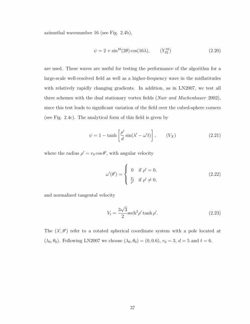
azimuthal wavenumber 16 (see Fig. 2.4b),

ψ = 2 + sin16(2θ) cos(16λ), (Y 1632 ) (2.20)

are used. These waves are useful for testing the performance of the algorithm for a

large-scale well-resolved field as well as a higher-frequency wave in the midlatitudes

with relatively rapidly changing gradients. In addition, as in LN2007, we test all

three schemes with the dual stationary vortex fields (Nair and Machenhauer 2002),

since this test leads to significant variation of the field over the cubed-sphere corners

(see Fig. 2.4c). The analytical form of this field is given by

ψ = 1− tanh

[ρ′

dsin(λ′ − ω′t)

], (VX) (2.21)

where the radius ρ′ = r0 cos θ′, with angular velocity

ω′(θ′) =

0 if ρ′ = 0,

Vtρ′

if ρ′ 6= 0,(2.22)

and normalized tangental velocity

Vt =3√

3

2sech2ρ′ tanh ρ′. (2.23)

The (λ′, θ′) refer to a rotated spherical coordinate system with a pole located at

(λ0, θ0). Following LN2007 we choose (λ0, θ0) = (0, 0.6), r0 = 3, d = 5 and t = 6.

37

Figure 2.4:Contours of the analytical function (a) Y 2

2 , (b) Y 1632 , and (c) the vortex

fields with one of the vortices centered about (λ0, θ0) = (0, 0.6). Dottedlines show the regular latitude-longitude grid.

38

2.4.2 Error measures

The performance of the algorithm is quantified using standard error measures:1

l1 ≡I(∣∣ψnum − ψexact∣∣)

I(ψexact

) , (2.24)

l2 ≡

√I[(ψnum − ψexact

)2]

√I[(∣∣ψexact∣∣)2

] , (2.25)

l∞ ≡max

(∣∣ψnum − ψexact∣∣)max

(∣∣ψexact∣∣) , (2.26)

where I is the global integral

I(f) =∑n

fnAn. (2.27)

The numerically generated “exact” solution

fn =1

An

∫An

fdA, (2.28)

is computed by fourth-order Gaussian quadrature. One finds that the error measure

l1 tends to identify the error in large-scale features of the field, whereas as p → ∞

the errors that are described by the norm become increasingly localized.

2.4.3 Calculation of reconstruction coefficients

Calculation of the reconstruction coefficients a(p,q) that describe the sub-grid cell

reconstruction is required for the second- and third- order schemes. Recall that the

grid is an equiangular cubed-sphere grid that, when translated to Gnomonic coor-

dinates, leads to cell centroids that are far from equidistant. As a consequence,

1Note that the `2 error employed in LN2008 corresponds to (`2)2.

39

if applied in Gnomonic coordinates, an equidistant discrete derivative operator will

lead to large derivative errors. We examine two possible solutions to this problem:

First, we can compute the derivatives in equiangular coordinates using an equidis-

tant discrete derivative operator and then apply a stretching factor to obtain the

derivatives in Gnomonic coordinates. Second, we can use a non-equidistant discrete

derivative operator in Gnomonic coordinates. These methods will be compared, in

terms of the resulting error measures, in section 2.4.2.4.5.

We briefly discuss the method of computing the reconstruction coefficients via the

non-equidistant fitting in Gnomonic coordinate space. In general, these coefficients

can be computed by fitting a parabola through the neighbouring centroids, where we

have assumed that these centroids take on the cell-averaged value, and extracting the

reconstruction coefficients from the quadratic coefficients. If we define

∆xL = xi−1 − xi, and ∆xR = xi+1 − xi, (2.29)

it follows that a parabola p(x) fitted through the points (xi−1, yi−1), (xi, yi) and

(xi+1, yi+1) will satisfy

(∂p

∂x

)i

=(yi−1)(∆xR)2 − (yi) ((∆xR)2 − (∆xL)2)− (yi+1)(∆xL)2

(∆xR)(∆xL)(∆xR −∆xL), (2.30)

and

1

2

(∂2p

∂x2

)i

=(yi−1)(∆xR)− (yi) (∆xR −∆xL)− (yi+1)(∆xL)

(∆xR)(∆xL)(∆xL −∆xR). (2.31)

Note that the discretized derivatives (2.30) and (2.31) reduce to the usual central

difference discretization in the case of equispaced grid points (∆xL = −∆xR). A

discretization for the third-order cross term (∂2f/∂x∂y)n can be easily calculated

on repeatedly applying (2.30) in each coordinate direction. It is simple but math-

ematically intensive to extend this method to higher orders by fitting a quartic or

40

Figure 2.5:A depiction of the halo region along the boundary of the top panel (dashedlines), showing the overlap with cells of the neighbouring panels. Observethat accurate modeling of the halo region only requires 1D interpolationfor this choice of grid.

higher-order curve, and so the resulting formula is not presented here.

Although both the parabolic fit (3-point) and quartic fit (5-point) can be used to

derive reconstruction coefficients for the third-order scheme, we have chosen to use

the 3-point stencil for the second-order scheme and the 5-point stencil for the third-

order scheme. This choice is made since the parabolic fit corresponds most closely to

a piecewise-linear reconstruction, whereas the quartic fit corresponds most closely to

the piecewise-parabolic reconstruction of Colella and Woodward (1984).

41

Note that when applying the discretized derivative operator in ABP coordinates,

halo regions must be provided for cells along the boundary of each panel. These

halo cells should correspond to the cells that would be obtained by extending each

panel outward, overlapping cells of the neighbouring panels (see Fig. 2.5). Hence,

halo cells do not exactly correspond to boundary cells on the neighbouring panels,

and their cell-averaged values must be obtained via a 1D remapping. Note that this

1D remapping does not require that the conservation criteria be fulfilled, since the

area-averaged property of the interior cells is satisfied for any choice of reconstruction

coefficients. For our purposes, we obtained the best accuracy from a straightforward

fourth-order non-conservative cubic fit.

2.4.4 Discussion

The error measures associated with remapping from the equiangular cubed-sphere

grid to RLL grid are given in Figures 2.6 and 2.7, for a high-resolution cubed-sphere

grid (Nc = 80 grid lines on each panel) and a medium-resolution cubed-sphere grid

(Nc = 40) mapped to a RLL grid with Nλ = 128 longitudes and Nθ = 64 latitudes.

The results of remapping from the same RLL grid (Nλ = 128, Nθ = 64) to a high-

resolution cubed-sphere grid (Nc = 80) are given in Fig. 2.8.

It should be emphasized that, in each case, the GECoRe method should perform

at least as well as SCRIP, since both methods lead to a derivative error that should

be roughly identical for PCoM and PLM. The two methods deviate only in their

geometric error, in that the geometrically exact techniques used for GECoRe lead

to geometric error that is roughly on the order of machine epsilon. It should be

noted that slight deviations from machine epsilon occur in GECoRe due to poorly

conditioned function evaluations in some of the antiderivatives (that is, calculations

involving the difference of two nearly equal floating point numbers, or evaluations of

arcsin or arccos near ±1), but for our purposes we can assume these deviations are

42

PCoM PLM PPM10−8

10−6

10−4

10−2

PCoM PLM PPM10−8

10−6

10−4

10−2

PCoM PLM PPM10−8

10−6

10−4

10−2

PCoM PLM PPM10−6

10−4

10−2

PCoM PLM PPM10−6

10−4

10−2

PCoM PLM PPM10−5

10−4

10−3

10−2

PCoM PLM PPM10−6

10−5

10−4

10−3

PCoM PLM PPM10−5

10−4

10−3

10−2

PCoM PLM PPM10−5

10−4

10−3

10−2

GECoRe SCRIP CaRS

l1 Error l

2 Error l∞ Error

Y22

Y1632

VX

Figure 2.6:Performance measures for the remapping of Y 2

2 , Y 1632 and the idealized

vortices (VX) from a medium-resolution ABP grid (Nc = 80) to a RLL grid(Nλ = 128, Nθ = 64) using GECoRe, SCRIP and CaRS with piecewiseconstant (PCoM), piecewise linear (PLM) and piecewise parabolic (PPM)reconstructions.

43

PCoM PLM PPM10−8

10−6

10−4

10−2

PCoM PLM PPM10−6

10−5

10−4

10−3

PCoM PLM PPM10−6

10−4

10−2

PCoM PLM PPM10−4

10−3

10−2

PCoM PLM PPM10−4

10−3

10−2

PCoM PLM PPM10−4

10−3

10−2

10−1

PCoM PLM PPM10−5

10−4

10−3

10−2

PCoM PLM PPM10−4

10−3

10−2

PCoM PLM PPM10−3

10−2

10−1

GECoRe SCRIP CaRS

l1 Error l

2 Error l∞ Error

Y22

Y1632

VX

Figure 2.7: As Fig. 2.6, except with Nc = 40.

44

PCoM PLM PPM10−5

10−4

10−3

10−2

PCoM PLM PPM10−5

10−4

10−3

10−2

PCoM PLM PPM10−4

10−3

10−2

PCoM PLM PPM10−4

10−3

10−2

PCoM PLM PPM10−4

10−3

10−2

10−1

PCoM PLM PPM10−3

10−2

10−1

PCoM PLM PPM10−4

10−3

10−2

PCoM PLM PPM10−3

10−2

10−1

PCoM PLM PPM10−2

10−1

GECoRe SCRIP CaRS

l1 Error l

2 Error l∞ Error

Y22

Y1632

VX

Figure 2.8:As Fig. 2.6, except remapping from a RLL grid (Nλ = 128, Nθ = 64) toan ABP grid (Nc = 80).

45

effectively negligible.

As expected, all error norms for SCRIP, CaRS and GECoRe tend to decrease

when going from PCoM to PLM to PPM. We expect that extending these methods by

including the piecewise cubic scheme (PCM, as done for CaRS in LN2008) and higher-

order reconstructions will lead to smaller, and perhaps worthwhile, improvements in

the accuracy of the method (Figs. 2.6, 2.7, 2.8).

For the first-order piecewise constant method, we observe nearly identical be-

haviour for GECoRe and SCRIP since, in both cases, line segments are effectively

integrated along constant fields. Hence, small perturbations in the geometrical orien-

tation of the line segments will not lead to significant differences in the resulting line

integral.

However, we find that the error measures in GECoRe and SCRIP deviate sig-

nificantly for the second- and third-order methods. The effect of geometric error is

clearly apparent in our calculations, as GECoRe produces results that are often one

or two orders of magnitude better than the associated error from SCRIP. The results

are particularly apparent for the smooth field Y 22 , where each of the error measures

shows an improvement of two to four orders of magnitude.

Comparing the spatial distribution of error for the three schemes (see Fig. 2.9),

we observe that the error for SCRIP and CaRS tends to be most significant near the

corners, whereas GECoRe has a much more uniform distribution of the resulting error.

This result reflects the lack of a contribution from geometric error in the GECoRe

scheme, which tends to dominate near the singularities of the cubed-sphere grid.

Hence, we can further conclude that, compared to SCRIP and CaRS, the GECoRe

scheme tends to be affected less strongly by the shape of the underlying grid.

46

Figure 2.9:Spatial distribution of the error (×10−2) for the remapping of Y 16

32 from acoarse-resolution ABP grid (Nc = 40) to a RLL grid (Nλ = 128, Nθ = 64)using (a) GECoRe, (b) SCRIP and (c) CaRS with piecewise parabolic(third-order) reconstructions. Both SCRIP and CaRS show clear corre-lation between the errors are the underlying cubed-sphere grid, whereasthis “grid imprinting” is reduced under the GECoRe scheme.

2.4.5 Impact of the reconstruction method

We briefly turn our attention to derivative error in the GECoRe schemes by com-

paring four methods for computing the reconstruction coefficients in each cell. We

focus on the non-equidistant parabolic fit (3-point) and quartic fit (5-point) methods,

both computed in Gnomonic coordinates, to the stretched equidistant 3-point and

5-point methods computed in equiangular coordinates. Results from this comparison

are given in Fig. 2.10.

Observe that there is no significant difference between both 3-point schemes and

both 5-point schemes for the non-smooth Y 1632 and VX test cases, since the natural

derivative error dwarfs any error that would be present from stretching of the equian-

gular reconstruction. However, for the smooth test case, there are obvious deviations

between the four methods in the third-order PPM scheme. In particular, we clearly

observe an immediate benefit to computing the reconstruction coefficients directly in

47

PLM PPM10−8

10−7

10−6

10−5

PLM PPM10−7

10−6

10−5

PLM PPM10−7

10−6

10−5

10−4

PLM PPM10−6

10−5

10−4

PLM PPM10−6

10−5

10−4

PLM PPM10−5

10−4

10−3

PLM PPM10−6

10−5

10−4

PLM PPM10−5

10−4

PLM PPM10−5

10−4

10−3

3−St 5−St 3−NE 5−NE

l1 Error l

2 Error l∞ Error

Y22

Y1632

VX

Figure 2.10:Performance measures for the remapping of Y 2

2 , Y 1632 and the idealized

vortices (VX) from a high-resolution ABP grid (Nc = 80) to a RLL grid(Nλ = 128, Nθ = 64) using GECoRe with four choices of sub-grid scalereconstruction techniques: 3-point stretched equiangular (3-St), 5-pointstretched equiangular (5-St), 3-point non-equidistant Gnomonic (3-NE)and 5-point non-equidistant (5-NE).

48

Gnomonic coordinates. From the non-smooth test cases we also observe an obvious

benefit to increasing the stencil size.

2.4.6 Impact of the monotone filter

In order to ensure monotonicity in the reconstruction, we employ the monotone

filter of Barth and Jespersen (1989). This simple monotone filter simply scales the

sub-grid scale reconstruction so that its minimum and maximum values do not exceed

the cell-averages of the neighbouring cells. In the case of the second-order linear

reconstruction, the extreme values within a cell will occur at the four corner points.

For the third-order reconstruction, the extrema could also possibly occur along the

boundary or within the cell. Hence, five additional points must be checked in the

third-order scheme.

The effect of applying the monotone filter to the remapping scheme is given in Fig.

2.11. We observe that this simple monotone limiter tends to reduce the accuracy of

the method by an order of magnitude, but, as a consequence, clearly maintains that

global extreme points are not enhanced. Tests performed on a simple cosine hill field,

which is more susceptible to overshoots and undershoots, actually result in improved

accuracy of the remapped field under the monotone limiter (not shown).

As resolution is increased, we expect that the loss of accuracy due to the monotone

limiter will be reduced, since higher resolution results in less relative variation in the

scalar field. Further, advanced limiters, such as that of Zerroukat et al. (2005), if

extended to two dimensions, are certain to result in an improved accuracy of these

results.

2.5 Summary

A general modeling environment consists of different model components, usually

implemented on different grid systems. Hence, accurate translation of scalar field

49

PLM PPM10−8

10−7

10−6

10−5

PLM PPM10−7

10−6

10−5

PLM PPM10−7

10−6

10−5

10−4

PLM PPM10−6

10−5

10−4

PLM PPM10−6

10−5

10−4

PLM PPM10−5

10−4

10−3

PLM PPM10−6

10−5

10−4

PLM PPM10−5

10−4

10−3

PLM PPM10−5

10−4

10−3

10−2

Non−Monotone Monotone

l1 Error l

2 Error l∞ Error

Y22

Y1632

VX

Figure 2.11:Performance measures for the remapping of Y 2

2 , Y 1632 and the idealized

vortices (VX) from a high-resolution ABP grid (Nc = 80) to a RLL grid(Nλ = 128, Nθ = 64) using GECoRe with (dotted line) and without(solid line) monotone filtering.

50

data between grid systems is important in order to ensure overall accuracy of the

model. For variables such as fluxes conservation is a particularly important property

that should also be maintained by the remapping scheme, as it ensures that a given

model does not disobey the fundamental laws of nature. The accuracy of existing

conservative schemes, such as SCRIP (Spherical Coordinate Remapping and Inter-

polation Package) and CaRS (Cascade Remapping between Spherical grids) is often

limited by the capacity of these methods to accurately model the geometry of the

problem. Here we have presented a high-order geometrically exact scheme for conser-

vative and monotone remapping of scalar fields between the regular latitude-longitude

and gnomonic cubed-sphere geometries. The new remapping scheme is referred to as

GECoRe (Geometrically Exact Conservative Remapping).

GECoRe is based on the principle that we can integrate certain fields in exact

closed-form along grid lines in the gnomonic cubed-sphere grid and regular latitude-

longitude grid. The advantage of this approach is the removal of geometric error

associated with low-order approximations to line segments at a similar computational

cost to existing techniques. Here we provide mechanisms for constructing schemes up

to third-order, possibly combined with an inexpensive monotone filter.

GECoRe is validated by remapping a standard set of both smooth and rapidly

varying test functions. Standard error measures are compared with existing SCRIP

and CaRS schemes at low and medium resolutions of the cubed-sphere grid. We

observe that the GECoRe scheme excels in both cases when applied at second-order

or higher, often yielding a one or two order of magnitude improvement over the

existing schemes without additional tweaking. However, SCRIP is more general than

GECoRe, since it can, in principle, handle any kind of spherical grids. Generalized

versions of GECoRe can be obtained by replacing the exact integrals, where the

exact formulas are too complicated or do not exist, with Gaussian quadrature of the

potentials (Lauritzen et al. 2008).

51

This work can be found in Ullrich et al. (2009).

52

CHAPTER III

Wave Reflection

3.1 Introduction

The atmosphere and ocean are two facets of a vast nonlinear system that works

on a broad range of interacting scales. Models are an invaluable tool for enhancing

our understanding of this system, but the immensity of the problem – spanning the

entirety of the Earth’s surface – is at the edge of our present computational power. In

order to meet growing demand for fine-scale simulations, the next generation of atmo-

spheric models will likely need to rely on adaptive mesh refinement (AMR) in order

to properly capture features of interest. A dynamically adaptive model, for instance,

would be capable of hurricane tracking and modeling on a global scale, and would

enhance our knowledge of mountain waves and extreme weather events. However, the

benefits of adaptively refined grids do not come without a fair share of problems. Per-

haps the most significant of these problems, in the context of geophysical modeling, is

related to the mathematical handling of wave phenomena at coarse-fine grid bound-

aries. Except for a handful of numerical methods, most schemes allow wave groups

to be spuriously reflected at grid resolution interfaces (see, for example, Vichnevetsky

(1987)). This type of wave reflection is attributed to sudden changes in the numerical

structure of the system, analogous to changes in the physical characteristics of the

system.

53

As shown by Vichnevetsky (1987) and later by Vichnevetsky and Turner (1991),

the significance of wave reflection increases substantially when the grid resolution is

varied abruptly. As a consequence, many approaches (see, for example, Cote et al.

(1998); Fox-Rabinovitz et al. (2001); Staniforth and Mitchell (1978)) instead rely on

a smooth variation of the grid between coarse and fine regions. However, abruptly-

varying grids generally perform better on parallel architectures when dynamic re-

finement is desired; in this case, dynamic grid refinement in a compact region can

be performed without having to reconstruct the grid over a wide regional or global

scale (which is necessary if smooth variation of the grid is required). Although these

block-adaptive grids have been long used for astrophysical, aerospace and other com-

putational fluid dynamics problems (see, for example, Berger and Colella (1989);

Berger and Oliger (1984)), they were only first applied to geophysical limited area

models by Skamarock et al. (1989) and Skamarock and Klemp (1993). More recently,

these methods have been applied in spherical geometry by Jablonowski et al. (2006)

and Jablonowski et al. (2009). Hence, our approach in this chapter is to consider only

grids with abrupt variation in resolution.

To a close approximation, the atmosphere and ocean are in a state of geostrophic

and hydrostatic balance. For geophysical flows, departures from geostrophy are ap-

proximately linear. The Mach number of these flows is generally much less than one,

and shock waves are not present. It is here where linear numerical discretizations

are the most relevant, since slope limiters are generally not required to ensure pos-

itivity of the thermodynamic variables. Long-term simulations of geostrophic flows

also require perhaps the most stringent conservation constraints since a slow escape

of air from the atmosphere on the order of the scheme’s truncation error can lead to

substantial atmospheric loss over time.

Although many previous papers have discussed the issue of wave reflection due to

a discontinuity in grid resolution, these works have not focused on the issue of wave

54

reflection in dissipative finite-volume methods. In this case, energy is not conserved

over time, and so it is uncertain whether previous results, which have been derived

in the case of zero energy dissipation, will still hold. Hence, it is our objective in this

chapter to use mathematical analysis and numerical experimentation to determine

which unstaggered dissipative finite-volume methods are best suited for geophysical

modeling in the presence of a refined grid.

Before proceeding, we briefly discuss the wave reflection properties of other ap-

proaches. Frank and Reich (2004) demonstrated that the Box scheme is free of spuri-

ous reflections, but this scheme does not easily generalize to multiple dimensions and

is implicit in a periodic domain. Further, purely upwind schemes, such as the first-

order Godunov scheme, the discontinuous Galerkin (DG) scheme and spectral-volume

methods, all of which do not use downstream information, are free from spurious wave

reflection when applied to the advection equation. Nonetheless, these methods still

suffer from nonlinear wave reflection when applied to the 1D shallow-water equations,

for instance.

The foundation for our analysis will be the 1D advection equation, which describes

the motion of a tracer field q(x, t) in the presence of an underlying velocity field u.

In its simplest form, this equation reads

∂q

∂t+ u

∂q

∂x= 0. (3.1)

For simplicity, much of our analysis will be for the case that u = const > 0.

This paper is organized as follows. First, we present a framework for the set of

finite-volume methods we will consider in section 3.2, and give some of their numerical

properties. The results of a set of wave-reflection experiments are then given in section

3.3. In section 3.4 we introduce the shallow-water equations and linearized shallow-

water equations, and show their connection to the advection equation. Lastly, our

55

conclusions are presented in section 3.6. Note that throughout this chapter we will

be making use of dimensionless length and time units.

3.2 Numerical discretizations

Numerous methods have been devised for the construction of finite-volume schemes,

and all have their benefits and disadvantages. The method-of-lines approach is per-

haps the most popular for constructing high-order finite-volume methods that are

applicable to general systems of equations. Under this framework, a spatial sub-

grid-scale reconstruction is combined with a numerical flux function to provide a

discretization of the spatial component of the differential equation, which is then

combined with a timestepping scheme that guarantees stability and accuracy when

integrating forward in time. Timestepping schemes vary substantially in their proper-

ties, but must be chosen so that the eigenvalues of the spatial operator fit within the

stability region of the timestepping scheme. We consider three types of finite-volume

methods constructed under this framework:

• Symmetric finite-volume. If we assume continuity of our solution between

elements we can directly reconstruct the value of the underlying field at edge-

points. An interior reconstruction, which is necessary for evaluating source

terms, is then obtained from the edge-values and value of the cell-averaged

scalar field. Once the initial approximation is made, monotonicity constraints

can be applied, which may cause the field to again become discontinuous at

edges and hence require the solution of a Riemann problem. This approach

does not rely more strongly on upwind-biased information, and so leads to

a spatial discretization which is symmetric about the element being updated.

The simplest symmetric finite-volume method is the so called central-in-space

discretization, which has been thoroughly studied in the context of grid reflec-

56

tion (see, for example, Trefethen (1982); Vichnevetsky (1987); Vichnevetsky and

Turner (1991)). It is obtained by assuming the value of the scalar field at each

edge is simply the average of the values of neighbouring elements.

• Upwind finite-volume. The Monotone Upstream-centered Schemes for Con-

servation Laws (MUSCL) formalism of van Leer (1979) provides a mechanism

for computing a sub-grid-scale reconstruction via a local reconstruction obtained

from adjacent cell-averaged values. When evaluated at edge points, these re-

constructions can then act as left and right states that are then used to solve a

Riemann problem. Slope limiters can also be applied in the reconstruction step

to enforce monotonicity and limit spurious oscillations. This approach leads to

the upwind family of finite-volume schemes, so-named because they rely more

heavily on information propagated in the direction of the fluid motion. Unstag-

gered high-order upwind finite volume schemes have been recently shown to be

viable for shallow-water models on the sphere by Ullrich et al. (2010).

• Semi-Lagrangian integrated-mass (SLIM) finite-volume methods. A

popular method that has been widely adopted for discretizations of the advec-

tion equation is the semi-Lagrangian (SL) approach. This method comes in two

flavors – namely, forward SL and backward SL. In the forward SL approach,

the velocity field is used to deform the grid, which is then remapped back to

the original cell positions. In the backward approach, the velocity field is first

evolved to time n+ 1. The evolved velocity field is then used to “devolve” the

grid cells at time n + 1 into a deformed grid that represents the locations of

these cells at time n. Finally, the original grid information is remapped onto

the deformed grid, giving new cell averages. These two approaches are identi-

cal for the 1D advection equation with u = const. Semi-Lagrangian methods

are a physically motivated treatment of the advection equation, and have effec-

57

tively no timestep limit (but accuracy degrades substantially for large timesteps

and non-constant flow fields). Nonetheless, there is some difficulty in adapting

this method to general hyperbolic systems. An analysis of SLIM schemes can

be found in Laprise and Plante (1995). Examples of this approach include

Fromm’s scheme Fromm (1968), the advective form of the piecewise-parabolic

method presented by Colella and Woodward (1984) and, in higher dimensions,

the recently introduced CSLAM transport scheme of Lauritzen et al. (2010).

3.2.1 Diffusion, phase velocity and group velocity

An excellent tool for describing the properties of numerical discretizations is wave-

mode analysis, which forms the backbone of our study of spurious wave reflection.

In particular, this approach has been successfully applied by Trefethen (1982) and

Grotjahn and O’Brien (1976) in the analysis of numerical methods for hyperbolic

equations.

In general, any linear partial differential equation with constant coefficients sup-

ports wave-like solutions of the form

q(x, t) = q exp(i(kx− ωt)), (3.2)

where q(x, t) denotes the state variable in physical space, q is the corresponding

amplitude, k is the wave number and ω is the frequency. If we substitute this solution

into (3.1) we obtain a dispersion relation of the form

ω(k) = uk. (3.3)

These modes propagate with speed

cp(k) =ω(k)

k, (3.4)

58

which is known as the phase speed. The evolution of a wave packet however, is

determined by the group speed, defined via

cg(k) =∂ω

∂k. (3.5)

It is well-known (see, for example, Brillouin (1960)) that the group speed is the

speed at which energy propagates in a system, as well as the speed associated with

a traveling wave packet. In the case of the advection equation, these velocities are

equivalent and given by cp = cg = u.

Linear discretizations of (3.1) similarly support wave modes of the form (3.2) but

only allow us to roughly approximate the correct dispersion relation (3.3). When

analyzing these numerical methods we will assume a uniform spatial grid, defined at

discrete points via

xj = j∆x, and tn = n∆t, (3.6)

where ∆x and ∆t are the element width and timestep, respectively, and j and n are

spatial and temporal indices. Hence, wave-like solutions (3.2) take the form

qnj = q exp(i(kj∆x− ωn∆t)), (3.7)

where k∆x is the normalized wave number, whose real component takes on values

in the range [0, π]. On substituting this expression into a discrete numerical scheme,

we obtain the numerical dispersion relation, which describes the relationship between

ω and k and usually incorporates the dimensionless Courant-Friedrichs-Lewy (CFL)

number

K =u∆t

∆x. (3.8)

The numerical dispersion relation is a powerful tool for describing the properties of a

numerical method:

59

• For two time-level schemes, such as forward Euler, backward Euler, Crank-

Nicolson and all Runge-Kutta schemes, every value of k is associated with a

single value ω. For three time-level schemes, such as the Leapfrog scheme,

every value of k is associated with two values of ω.

• The imaginary component of ω(k) describes the growth rate of the mode k.

Von Neumann stability Charney et al. (1950) is obtained by guaranteeing that

Im(ω) ≤ 0 for all real wave numbers. Stable numerical schemes which satisfy

Im(ω(k)) < 0 for some k are known as diffusive (or dissipative). Note that the

advection equation is naturally non-diffusive, so any non-zero diffusivity leads

to diffusive error. The amplification factor after one timestep is then defined

as

A∆t = exp(Im(ω(k))∆t). (3.9)

However, A∆t is not desirable for describing the diffusivity of a scheme over a

range of CFL numbers, since schemes with smaller timestep ∆t must be applied

multiple times to advance to the same time as schemes with larger ∆t. Hence,

one can alternatively describe diffusivity in terms of the normalized amplification

factor A, defined for a fixed wavenumber k by

A = exp(Im(ω(k))T ), (3.10)

where T is some fixed time. In the following analysis we choose T = 1 for

simplicity.

• In general, a numerical dispersion relation will yield a frequency whose real

component is nonlinearly dependent on k. In this case, the scheme will be

dispersive, indicating that different wave numbers will travel at different phase

speeds. The advection equation is non-dispersive, since ω and k are linearly

60

related, however, numerical discretizations generally introduce dispersive error

in the form of a nonlinear dispersion relation. The dispersive characteristics of

a numerical method can be effectively described in terms of the phase velocity

and group velocity, which are obtained from the numerical dispersion relation,

when combined with (3.4) and (3.5). Since a numerical method can also be

dissipative, we substitute Re(ω) for ω in these relationships, which yields the

numerical phase velocity and group velocity.

Note that group velocity analysis only applies directly for nondiffusive schemes,

since diffusivity introduces a wavenumber-dependent attenuation of different wave

modes. As a consequence, wave packets can lose their distinctive shape over time as

certain wave modes are diffused from the simulation. However, the results of group

velocity analysis will still hold approximately as long as the wave packet is composed

of waves with similar diffusion rates.

3.2.2 Linear discretizations

In this chapter we focus our attention on high-order linear discretizations. Namely,

we are interested in spatial semi-discretizations of the advection equation (3.1) that

take the form

∂qj∂t

=r∑

m=−`

cmqj+m, (3.11)

where the coefficients cm are purely a function of the grid spacing ∆x, timestep ∆t

and advection speed u (possibly via the CFL number). Here ` and r denote the

number of leftward-elements and rightward-elements in the semi-discrete stencil. For

simplicity, in this chapter we only analyze methods with r ≤ ` = 2, which leads

to a stencil with at most five elements. Conservation is guaranteed by utilizing the

finite-volume framework, which requires that all of the schemes can be written in the

61

form

∂qj∂t

= −F ∗j+1/2(. . . , qj−1, qj, qj+1, . . .)− F ∗j−1/2(. . . , qj−1, qj, qj+1, . . .)

∆x, (3.12)

for a numerical flux function F ∗j+1/2. The numerical flux functions are defined at cell

edges, which are denoted by half-indices.

When combined with an appropriate two-time-level explicit timestepping opera-

tor, the spatial semi-discretization (3.11) then leads to a complete discretization of

the advection equation that we can write as

qn+1j =

r·s∑m=−`·s

Cmqnj+m, (3.13)

where the Cm are again purely functions of the grid spacing, timestep and advection

speed. Here s denotes the number of stages used by the timestepping operator (for

multistage schemes, such as the Runge-Kutta methods).

To determine the numerical dispersion relation for the scheme (3.13), we simply

substitute (3.7) and solve for ω, obtaining

ω = − 1

∆tarctan

r·s∑

m=−`·s

Cm sin(km∆x)

r·s∑m=−`·s

Cm cos(km∆x)

. (3.14)

Solutions to this equation are not unique, and the choice of an appropriate branch cut

for the arctan function can lead to some confusion. Herein we will take the branch

cut that gives ω(0) = 0 and otherwise is a continuous function of k.

62

3.2.3 The 2∆x mode problem

Symmetric finite-volume (semi-) discretizations of the advection equation satisfy

the property cm = −c−m, which usually arises from the application of a centered

differencing operator within each element. They are characterized by low diffusivity

and consistent behaviour regardless of CFL number, but suffer from the 2∆x mode

problem; namely, under such a semi-discretization both the constant field qj = const.

and the 2∆x mode qj = (−1)j satisfy

∂qj∂t

= 0, (3.15)

implying that both modes are invariant in time. Thus, under a symmetric finite-

volume method, the constant mode and 2∆x mode are indistinguishable, regardless

of the size of the stencil and choice of temporal discretization. As a consequence,

this mode will feature both zero diffusion and zero phase velocity when simulating

the advection equation, and so any nonlinear effects or source terms which contribute

energy to this scale will not be dissipated. The result is “checkerboarding” of the

state variables under this operator (see, for example, Randall (1994)).

Upwind finite-volume (semi-) discretizations are always upwind biased, satisfying

r < `. This criterion implies that more information is drawn from the upwind direc-

tion as the flow evolves. In general, these methods do not suffer from the 2∆x mode

problem, but may possess high-frequency wave modes which are weakly damped,

usually at specific CFL numbers.

3.2.4 The gas dynamics form of the piecewise-parabolic method (PPM)

The gas dynamics form of the piecewise-parabolic method (PPM) of Colella and

Woodward (1984) (Chapter 3) is a high-order symmetric discretization that, for a

63

locally smooth field q, estimates the field at edge points via the central reconstruction

qj+1/2 =−qj−1 + 7qj + 7qj+1 − qj+2

12+O(∆x4). (3.16)

Because the field is assumed continuous at edge points (with no limiter applied), the

numerical flux can be computed directly without applying a Riemann solver,

F ∗j+1/2 = u · qj+1/2. (3.17)

This choice leads to the semi-discretization

∂qj∂t

= −K∆t

(1

12qj−2 −

8

12qj−1 +

8

12qj+1 −

1

12qj+2

), (3.18)

where the RHS of (3.18) is exactly the fourth-order symmetric approximation to

∂q/∂x centered at element j. The eigenvalues of this spatial operator are purely

imaginary, and so must be paired with at least a three-stage third-order Runge-Kutta

(RK3) timestep. Doing so, we obtain a scheme that is stable up to K ≤ 1.26.

We plot the normalized amplification factor, group velocity and phase velocity

associated with this scheme in Fig. 3.1. Observe, in particular, that this scheme

supports waves with negative group velocity, leading to a maximum negative group

velocity of −5/3 at k∆x = π. The range of dimensionless wavenumbers k∆x ∈

[π/2, π] corresponds to the waves with wavelength between 4∆x and 2∆x. Most waves

in this range travel with negative group speeds and so are not truthfully represented

by the numerical scheme. Note that the phase velocity also drops to zero at k∆x = π,

whereas at this wavenumber the amplification factor is exactly 1 regardless of CFL

number. As mentioned previously, this implies that the 2∆x mode is an undamped

“standing wave” that is retained by the numerical method.

64

0.95

0.96 0.96

0.960.97

0.97

0.98

0.98

0.99

0.99

0.99

Amplification Factor

CF

L nu

mbe

r

π/4 π/2 3π/4 π0

0.2

0.4

0.6

0.8

1

1.2

−1

−1

−1

−0.5

−0.5

−0.5

0

00

0.5

0.5

0.5

1

Group Velocity (cg)

Dimensionless Wavenumber (k ∆ x)π/4 π/2 3π/4 π

0

0.2

0.4

0.6

0.8

1

1.2 0

00

0.2

0.2

0.4

0.4

0.6

0.6

0.8

0.8

1

Phase velocity (cp)

π/4 π/2 3π/4 π0

0.2

0.4

0.6

0.8

1

1.2

Figure 3.1:Contour plots showing diffusive and dispersive characteristics associatedwith PPM with RK3 timestep. Here ∆t is varied so as to span to CFLrange [0, 1.26] with constant wave speed u = 1 and fixed ∆x. Gray regionsin the group velocity plot indicate regions of negative group velocity.

3.2.5 A second-order upwind (FV2) scheme

A linear sub-grid-scale reconstruction was adopted by van Leer (1974, 1979)

for shock-hydrodynamics problems, where the derivative was obtained via a non-

linear limiting procedure. Without a strict monotonicity constraint, we can instead

forego the limiting procedure and hence obtain a linear second-order-accurate upwind

scheme. A sub-grid-scale reconstruction of the form

qj(x) = qj + (x− xj)Dqj, (3.19)

is computed in each cell, where Dqj denotes the numerical approximation to the first

derivative, obtained from the central-difference formula

Dqj =qj+1 − qj−1

2∆x. (3.20)

65

Since this reconstruction is discontinuous at cell edges we must use a Riemann flux

operator, taken simply to be the upwind flux

F ∗j+1/2 = uqj

(xj +

∆x

2

). (3.21)

After simplifying, the evolution equation reads

∂qj∂t

= −K∆t

(1

4qj−2 −

5

4qj−1 +

3

4qj +

1

4qj+1

), (3.22)

This scheme is unstable under a forward Euler timestep, but stable for Runge-Kutta

operators of at least second order. Making use of the two-stage second-order Runge-

Kutta scheme (RK2), we obtain a discretization that is stable for K ≤ 1.

We plot the normalized amplification factor, group velocity and phase velocity

associated with this scheme in Fig. 3.2. In particular, observe that for this scheme

wave modes which are propagated with negative group velocities are also modes which

experience strong diffusion. This result was previously obtained by Karni (1994),

who observed that even in the limit of vanishing CFL number wave groups were not

permitted to propagate backwards in upwind schemes. A singularity can also be

observed in the group velocity and phase velocity plots, corresponding to the point

where the amplification factor is identically zero. The solid line that extends to the

right of the singularity in the phase velocity plot is a discontinuity in the branch cut

when evaluating the frequency ω from (3.14). Comparing this scheme against PPM

in Fig. 3.1, we observe that the FV2 scheme possesses a much more complicated

structure and introduces stronger diffusion at high wavenumbers. As with PPM, the

2∆x mode is a standing mode with non-zero group velocity; however, unlike in PPM,

this mode is strongly damped at all but the largest of the stable CFL numbers. In

the nonlinear case this analysis suggests bounding the CFL number by 0.9 so as to

prevent artificial enhancement of this mode against the background field.

66

0.2

0.2

0.2

0.4

0.4 0.4

0.6

0.6

0.6

0.8

0.8

0.8 0.8

Amplification Factor

CF

L nu

mbe

r

π/4 π/2 3π/4 π0

0.2

0.4

0.6

0.8

1

−1

−1

−1

−0.5

−0.5

−0.5

0

0

0.5

0.5

0.5

1

1

1

1.5

2

2

Group Velocity (cg)

Dimensionless Wavenumber (k ∆ x)π/4 π/2 3π/4 π

0

0.2

0.4

0.6

0.8

1

−0.2

0

0 0

0.2

0.20.4

0.40.6

0.6

0.8

0.8

1

1

1.2

1.4

1.6

2

2.4 2.6

Phase velocity (cp)

π/4 π/2 3π/4 π0

0.2

0.4

0.6

0.8

1

Figure 3.2:Contour plots showing diffusive and dispersive characteristics associatedwith the FV2 scheme with RK2 timestep. Here ∆t is varied so as tospan to CFL range [0, 1] with constant wave speed u = 1. Gray regionsindicate regions of significant damping on the plot of the amplificationfactor (A ≤ 0.8) and negative (backwards propagating) group velocitieson the plot of the group velocity.

3.2.6 A third-order upwind (FV3p3) scheme

Extending on the ideas of van Leer (1974, 1977), we make use of a sub-grid-scale

reconstruction of the form

qj(x) = qj + (x− xj)Dqj +

((x− xj)2 − ∆x2

12

)(1

2D2qj

), (3.23)

where xj is the centerpoint of element j and Dqj and D2qj denote numerical ap-

proximations to the first and second derivatives of the field q in element j, obtained

from

Dqj =qj+1 − qj−1

2∆x, and D2qj =

qj+1 − 2qj + qj−1

∆x2. (3.24)

As with the FV2 scheme, we compute edge fluxes via the upwind flux (3.21), leading

to the evolution equation

∂qj∂t

= −K∆t

(1

6qj−2 − qj−1 +

1

2qj +

1

3qj+1

), (3.25)

67

0.2

0.2

0.2

0.4

0.4

0.4

0.4

0.40.6

0.6

0.6

0.60.

8

0.80.8

0.8

Amplification Factor

CF

L nu

mbe

r

π/4 π/2 3π/4 π0

0.2

0.4

0.6

0.8

1

1.2

1.4

1.6

−1

−1

−1

−1

−0.

5

−0.5

−0.5

−0.

5

00

0

0

0.50.5

0.5

1

1.5

2

2

Group Velocity (cg)

Dimensionless Wavenumber (k ∆ x)π/4 π/2 3π/4 π

0

0.2

0.4

0.6

0.8

1

1.2

1.4

1.60

0

0.2

0.2

0.4

0.4

0.4

0.60.6

0.6

0.8

0.8

1

1.2

2

Phase velocity (cp)

π/4 π/2 3π/4 π0

0.2

0.4

0.6

0.8

1

1.2

1.4

1.6

Figure 3.3:As Fig. 3.2 except with the FV3p3 scheme with RK3 timestep. Here wespan the CFL number over the range [0, 1.63].

This scheme is unstable under both the forward Euler method and RK2 timestep

since the eigenvalues of the spatial operator closely shadow the imaginary axis near

the origin. Hence, we will combine this spatial stencil with the third-order Runge-

Kutta (RK3) scheme, leading to a scheme that is stable up to K ≤ 1.63.

We plot the normalized amplification factor, group velocity and phase velocity

associated with this scheme in Fig. 3.3. As with the FV2 scheme (see Fig. 3.2),

the behaviour is complicated for wavenumbers in the range [π/2, π], featuring two

singularities due to the presence of a zero amplification factor. Again we observe a

similar branch cut discontinuity in the phase velocity plot. Interestingly, the group

velocity is positive for virtually all wavenumbers at K ≥ 1.32. Also, the 2∆x mode

always experiences significant diffusion under this scheme, whereas the 3∆x mode

(k∆x = 2π/3) is relatively undamped at high CFL numbers. Diffusion in this method

is comparable to the FV2 scheme, with slightly stronger diffusion at CFL numbers

greater than about 0.6.

68

3.2.7 A third-order semi-Lagrangian integrated-mass (SLIM3p3) scheme

The third-order semi-Lagrangian scheme we will analyze is based on the discon-

tinuous piecewise-parabolic reconstruction of Laprise and Plante (1995). In this case

we again make use of a reconstruction of the form (3.23) and (3.24), except now we

apply the SLIM methodology to compute fluxes by integrating upstream from each

cell edge. For CFL numbers in the range 0 ≤ K ≤ 1 the numerical flux function then

takes the form

F ∗j+1/2 =1

∆t

xj+∆x/2∫xj+∆x/2−u∆t

q(x′)dx′ (3.26)

=u

6

[(K2 − 1)qj−1 − (K + 1)(2K − 5)qj + (K − 1)(K − 2)qj+1

].

The integrated transport scheme then takes the form

∂qj∂t

= −K∆t

[−1

6(K2 − 1)qj−2 +

1

2(K + 1)(K − 2)qj−1 (3.27)

−1

2(K2 − 2K − 1)qj +

1

6(K − 1)(K − 2)qj+1

].

As stated earlier, SLIM methods can be extended to have an arbitrarily large CFL

number if the integration is applied only to elements that overlap the Lagrangian

control volume (see, for example, Lauritzen et al. (2010)).

Unlike (3.18), (3.22) and (3.25), the SLIM framework leads to an evolution equa-

tion that is nonlinear in K. This scheme is stable if combined with a forward Euler

timestep and further is exact for K = 1. Unlike the previous schemes, we do not rec-

ommended combining this scheme with a Runge-Kutta timestep since the resulting

scheme is highly diffusive.

We plot the normalized amplification factor, group velocity and phase velocity

associated with this scheme in Fig. 3.4. The remapping step in the SLIM framework

69

0.2

0.2

0.4

0.4

0.6

0.6

0.8

0.8

Amplification Factor

CF

L nu

mbe

r

π/4 π/2 3π/4 π0

0.2

0.4

0.6

0.8

1

−1

−1

−0.

5

−0.5

00.5

1

1.5

2

2

Group Velocity (cg)

Dimensionless Wavenumber (k ∆ x)π/4 π/2 3π/4 π

0

0.2

0.4

0.6

0.8

10

0.2

0.4

0.6

0.6

0.8

1.2

Phase velocity (cp)

π/4 π/2 3π/4 π0

0.2

0.4

0.6

0.8

1

Figure 3.4:As Fig. 3.2 except with the SLIM3p3 scheme with forward Euler timestep.Here we span the CFL number over the range [0, 1.0].

is responsible for the diffusivity of the scheme, and leads to an amplification factor of

zero at k = π and K = 12

(with a corresponding singularity in the group velocity). As

with the upwind finite-volume schemes, waves in the region of negative group velocity

also experience strong diffusion. Notably, diffusion in this scheme is weaker than for

the corresponding upwind schemes.

3.3 Wave reflection

In this section we tackle the problem of spurious wave reflection due to a grid res-

olution discontinuity. In section 3.3.1, we introduce our test environment for spurious

wave reflection. We analyze the decay rate of spurious modes in section 3.3.2 and

the initial amplitude of a reflected wave in section 3.3.3. We present several reflected

wave tests using a symmetric FV scheme in section 3.3.4 with and without a slope

limiter. A similar analysis is performed for upwind finite-volume schemes in section

3.3.5 and for SLIM finite-volume schemes in section 3.3.6.

Spurious wave reflection in the advection equation can be attributed to an artificial

transfer of energy from forward-propagating physical modes into spurious backward-

70

propagating parasitic modes. When a forward-propagating wave packet hits a res-

olution discontinuity, frequency must be conserved across the interface, but errors

are accumulated at all wave numbers with the supported frequency. Certain modes

are then propagated backwards relative to the flow. This type of wave reflection can

occur even when a scheme does not possess wave modes with negative group velocity,

and depends largely on the amount of downstream information that is used in the

evolution equations; it is a linear effect, and so tends to be the dominant source of

error even among nonlinear differential equations.

3.3.1 Wavemaker driven grid reflection

Wave-like solutions are not, in general, eigenfunctions of the discrete update equa-

tions on a grid with a resolution discontinuity. However, if we neglect boundary con-

ditions, they are eigenfunctions of the update equations on each uniformly spaced

grid.

In order to analyze wave reflection at grid resolution discontinuities, we follow the

approach proposed by Trefethen (1982). Under this simplified model, the advection

equation is simulated over a domain x = [0, 1] with a grid resolution discontinuity

introduced at x = 1/2. In the regions x = [0, 1/2] and x = [1/2, 1] we make use of

discrete grid spacing ∆xf (on the fine grid) and ∆xc (on the coarse grid), respectively,

with ∆xf < ∆xc. The resolution ratio R ≥ 1 at the discontinuity is then defined as

R =∆xc∆xf

. (3.28)

At time t = 0, we begin forcing the left boundary with real frequency ω and amplitude

A. As a consequence, we observe a wave of the form

q(x, t) = A exp(i(kx− ωt)), (3.29)

71

average reconstruct

fine grid

coarse grid

Figure 3.5:We maintain the illusion of resolution regularity by averaging from thefine grid to coarse grid ghost elements. To obtain the cell-averaged valueson the fine grid, we first construct a sub-grid-scale reconstruction on thecoarse grid and then integrate it to obtain the cell-averages on the finegrid. The dotted (overlapping) regions contain the ghost cells.

with complex wavenumber k(ω) satisfying Im(k) ≥ 0 (under sufficient stability con-

ditions).

When running simulations, the resolution discontinuity is treated much like any

other boundary on a uniform resolution domain (see Fig. 3.5). On both the fine

and coarse grid the boundary conditions at this point must be obtained from the

overlapping grid panel. As a consequence, we are able to maintain the illusion of grid

resolution uniformity during the simulation, as long as the boundary conditions are

correctly applied.

In order to obtain element-averages for the coarse grid ghost elements that are

consistent with the fine grid, we simply average from the fine grid elements. To

obtain element-averages on the fine grid from the coarse grid, we first build a sub-

grid-scale reconstruction of the form (3.23) using the element-averaged values from

the fine grid and known coarse grid element-averages. Piecewise-linear and piecewise-

constant reconstructions can alternatively be obtained by setting one or both of Dqj

or D2qj to zero. Then for each fine-grid ghost cell we average over the corresponding

reconstruction. This process easily generalizes to higher dimensions, and does not

require any additional special treatment of elements near the resolution discontinuity.

72

3.3.2 Decay of parasitic modes

The decay rate of the reflected wave modes can be determined directly from the

discretization. Once the initial perturbations from kick-starting the system have died

down the frequency ω becomes invariant. Hence, both the “true wave” and “parasitic

wave” must oscillate at frequency ω. To determine all complex wavenumbers k with

natural frequency ω, we assume wavelike solutions of the form (3.29). If we define

β = exp(ik∆x), unstaggered FV schemes of the form (3.13) can be reduced to a

polynomial of the form

(exp(−iω∆t)− 1)β` =r·s∑

m=−`·s

Cmβm+`. (3.30)

Hence, this polynomial will have r · s+ ` · s roots that represent all wavenumbers that

oscillate at frequency ω. In particular, if we assume sufficient stability conditions,

roots with Im(k) ≥ 0 will be decaying modes that are propagated forward by our

scheme, whereas roots that satisfy Im(k) < 0 will be growing modes that are propa-

gated backwards (these are the “parasitic modes”). In fact, the smaller in magnitude

(or closer to zero) we observe for Im(k), the longer the resulting “tail” is from the

point of generation. Hence, we define the dominant parasitic mode for an FV scheme

to be the mode k(ω) that satisfies (3.30) with Im(k) < 0 such that for any other

parasitic mode k′ we have Im(k) > Im(k′). The spatial decay rate of the dominant

parasitic mode is then defined as −Im(k∆x). A large positive decay rate leads to a

sharp drop-off of the parasitic mode, whereas a small positive decay rate leads to an

elongated tail. A decay rate of zero corresponds to a parasitic mode which does not

decay away from the resolution discontinuity.

We plot the dominant parasitic mode for various choices of frequency ω in Fig.

3.6. In general, the complexity of the polynomial (3.30) prevents us from obtaining

any general results in all but the simplest of cases, but we can nonetheless make some

73

observations based on these four schemes:

• In all cases the decay rate appears to be smallest at ω = 0, which is associated

with a constant forcing. The decay rate then increases monotonically as ω

increases.

• At ω = 0 the decay rate can be derived analytically if we observe that, for

the schemes we have analyzed, the dominant parasitic mode is the same if we

use the coefficients cm (see (3.11)) in place of Cm in (3.30). In fact, for the

two upwind schemes and the SLIM scheme with a forward Euler timestep, the

degree of the polynomial (3.30) is only three. If we further observe that for any

consistent scheme β = 1 (the constant mode) must be a root of (3.30), then the

remaining roots are

β =−(c0 + c1)±

√(c0 + c1)2 − 4c1(c−1 + c0 + c1)

2c1

. (3.31)

Using this formula, we can calculate that the ω = 0 decay rate of the dominant

parasitic mode is 1.44 ≈ log(−2 +√

5) for the FV2 scheme, 0.99 ≈ log((−5 +√

33)/2) for the FV3p3 scheme and

β =(2K2 − 3K − 5)−

√−15K2 + 18K + 33

2(K2 − 3K + 2), (3.32)

for the SLIM3p3 scheme. In the limit as K → 1, the SLIM3p3 scheme does not

have any parasitic modes, and so the decay rate tends to infinity. In the limit

as K → 0, the SLIM3p3 scheme converges to a decay rate of log((5 +√

33)/4).

Observe that since the coefficients cm are linear in K for the symmetric and

upwind FV schemes, all dependence on K divides out of (3.31).

• For the schemes that use pointwise edge values to calculate edge fluxes (namely,

PPM, FV2 and FV3p3), the decay rate decreases monotonically with increasing

74

0 π/4 π/2 3π/4 π

0

1

2

3

4

5

(0.1)

(0.5)

(1.0)(1.2)

(a) PPM

Dec

ay R

ate

0 π/4 π/2 3π/4 π

0

1

2

3

4

5

(0.1)

(0.5)

(1.0)

(b) FV2

0 π/4 π/2 3π/4 π

0

1

2

3

4

5

(0.1)

(0.5)

(1.0)

(1.6)

(c) FV3p3

0 π/4 π/2 3π/4 π

0

1

2

3

4

5

(0.2)

(0.5)

(0.9)

(d) SLIM3p3

Forcing frequency (ω ∆ t)

Figure 3.6:The decay rate (−Im(k∆x)) of the dominant parasitic modes for (a) PPM,(b) FV2, (c) FV3p3 and (d) SLIM3p3 under sinusoidal forcing of fre-quency ω and for several choices of CFL number (indicated in parenthesison each curve).

CFL number at all frequencies ω > 0. At ω = 0, we observe that the decay rate

is independent of CFL number.

The number of elements affected by the parasitic mode before it is damped below

a fixed threshold is independent of the grid spacing. For a decay rate of 1.44, as with

the FV2 scheme, a perturbation at the grid resolution interface of magnitude 1 will

require approximately 8 elements to be damped to 10−5. For a decay rate of 0.99, as

with the FV3p3 scheme, the same perturbation will require 12 elements to decay to

10−5.

3.3.3 Amplitude of the parasitic mode at the discontinuity

In addition to knowing the decay rate of a given parasitic mode, it is important to

also understand its initial amplitude at a grid resolution discontinuity. To study the

amplitude of the parasitic mode, we carried out a sequence of simulations using the

PPM scheme at forcing frequencies that were sufficiently low to prevent the parasitic

mode from decaying significantly (see Fig. 3.6). The amplitude of the parasitic mode

75

was calculated empirically by differencing the unrefined and refined grid simulations

near the grid resolution discontinuity. This result was then normalized by the ampli-

tude of the incident wave at the discontinuity (since, especially at high wave-numbers,

substantial decay of the incident mode was observed).

The empirically calculated ratio of the amplitude of the parasitic mode to the

amplitude of the incident wave is depicted in Fig. 3.7 for various simulations with

resolution ratios R = 2, 4 and 8. For waves that are well-resolved on both grids,

the initial amplitude of the parasitic mode at the discontinuity is largely due to the

discrepancy between the “true” solution on the fine grid and the solution in the over-

lapping grid elements obtained from remapping the coarse grid solution. Improving

the order of accuracy in the remapping stage (using a piecewise linear or piecewise

parabolic reconstruction, for instance, instead of a piecewise constant reconstruction)

will reduce the initial amplitude of the perturbation. For wavenumbers which are

poorly resolved or unresolved on the coarse grid, the reconstruction will not carry

any information about the “true” wave and so the discrepancy between the incident

wave and the representation on the coarse grid will be essentially maximal. In this

case, improving the formal accuracy of the remapping procedure will not improve the

outcome, since the element averages of the reconstruction on the coarse grid still do

not contain any information about these waves.

As observed previously in the literature (see, for example, Vichnevetsky (1987)),

wave reflection can be dramatically reduced by smoothly adjusting the grid spacing,

rather than through abrupt changes in resolution. Intuitively, this result follows since

the sub-grid-scale reconstruction on adjacent grid cells closely matches up under a

smoothly varying element width. This result is also consistent with the observations of

Trefethen (1982), who noted that forcing at the outflow boundary produced parasitic

modes of the same amplitude as the prescribed forcing.

For comparison, we have devised a simple model for predicting the parasitic am-

76

plitude. Our goal is to demonstrate that the discrepancy between the solution on the

uniform-resolution grid and the solution on the refined grid is the dominant influence

in determining the amplitude of the parasitic mode for well-resolved incident waves.

Given incident wave solution of the form (3.29), we can define a moving average

operator via

q(x;R,∆xf ) =1

R∆xf

x+R∆xf∫x

q(x)dx. (3.33)

If a wave is well-resolved on the fine grid, it will propagate without modification, and

so the element average on the fine grid qf will be given by

qf = q(x; 1,∆xf ) =exp(i(kx− ωt))

k∆xf(exp(ik∆xf )− 1). (3.34)

If the wave is well-resolved on the coarse grid as well, the corresponding element

average of the first element on the coarse grid qc will be

qc = q(x;R,∆xf ) =exp(i(kx− ωt))

Rk∆xf(exp(iRk∆xf )− 1). (3.35)

For a piecewise-constant reconstruction at the discontinuity, the discrepancy between

the true and approximate solution (copied directly from the coarse grid) is then given

by D = qf−qc. This approach can be easily extended to higher-order reconstructions

(such as we have done with the piecewise-parabolic reconstruction in Fig. 3.7), but

for sake of brevity we have not included the corresponding formula here.

Waves that are not well-resolved on both grids will deviate from the ideal propa-

gation model described above. As frequency is increased, we observe that these wave

modes will lead to greater reflection than the ideal model at almost the same frequency

for both reconstruction schemes. In fact, if we compare this point of departure with

the group velocity plots given in Fig. 3.1, we observe it is approximately correlated

with regions where the group velocity tends away from u = 1. Thus, for waves in

77

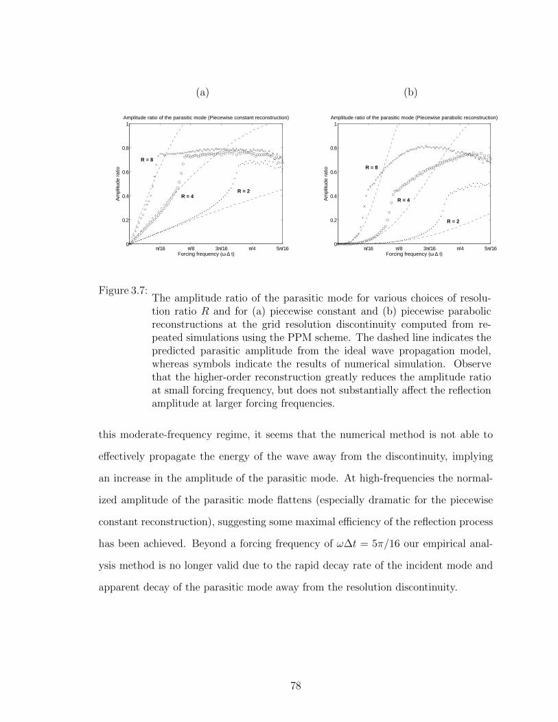
(a) (b)

π/16 π/8 3π/16 π/4 5π/160

0.2

0.4

0.6

0.8

1

Forcing frequency (ω ∆ t)

Am

plitu

de r

atio

Amplitude ratio of the parasitic mode (Piecewise constant reconstruction)

R = 8

R = 4R = 2

π/16 π/8 3π/16 π/4 5π/160

0.2

0.4

0.6

0.8

1

Forcing frequency (ω ∆ t)

Am

plitu

de r

atio

Amplitude ratio of the parasitic mode (Piecewise parabolic reconstruction)

R = 4

R = 8

R = 2

Figure 3.7:The amplitude ratio of the parasitic mode for various choices of resolu-tion ratio R and for (a) piecewise constant and (b) piecewise parabolicreconstructions at the grid resolution discontinuity computed from re-peated simulations using the PPM scheme. The dashed line indicates thepredicted parasitic amplitude from the ideal wave propagation model,whereas symbols indicate the results of numerical simulation. Observethat the higher-order reconstruction greatly reduces the amplitude ratioat small forcing frequency, but does not substantially affect the reflectionamplitude at larger forcing frequencies.

this moderate-frequency regime, it seems that the numerical method is not able to

effectively propagate the energy of the wave away from the discontinuity, implying

an increase in the amplitude of the parasitic mode. At high-frequencies the normal-

ized amplitude of the parasitic mode flattens (especially dramatic for the piecewise

constant reconstruction), suggesting some maximal efficiency of the reflection process

has been achieved. Beyond a forcing frequency of ω∆t = 5π/16 our empirical anal-

ysis method is no longer valid due to the rapid decay rate of the incident mode and

apparent decay of the parasitic mode away from the resolution discontinuity.

78

3.3.4 Wave reflection by symmetric FV schemes

As observed in Fig. 3.6, PPM does not significantly damp reflected oscillations

at any frequency. This result is apparent in any of the wave-driver simulations using

undamped PPM (see Fig. 3.8). Here we clearly observe a very strong, undamped

high-frequency wave that travels away from the grid resolution interface. The reflected

wave has a normalized wavenumber k∆x ≈ π and so travels at a group velocity of

≈ 5/3 (see Fig. 3.1). As a consequence, the parasitic mode has almost reached the

left boundary by the time the rightgoing wave has only traversed half of the coarse

domain.

In agreement with the results in section 3.3.3 we see that increasing the order of

accuracy of the remapping process at the resolution discontinuity does not signifi-

cantly affect the qualitative properties of the parasitic wave, and only has an effect

on the amplitude of the parasitic wave at smaller wavenumbers (see Fig. 3.9).

One might wonder if combining this symmetric scheme with a slope/curvature

limiter would be sufficient to remove spurious parasitic waves. If we apply the limiting

procedure described in Colella and Woodward (1984) we can no longer guarantee

continuity at cell edges, and so must utilize a Riemann flux where discontinuities

occur. In this case we adopt an upwind flux operator analogous to (3.21). Simulations

were again carried out using a unlimited piecewise parabolic reconstruction at the

resolution discontinuity and are plotted in Fig. 3.10. The oscillations have been

suppressed substantially in this case, but have not been removed completely. In fact,

in the small wavenumber case (ω = 20.0) we clearly see that the parasitic mode

is persistent at about 10−3 of the magnitude of the initial wave – we observe the

spurious mode is able to “hide” in the low-frequency incident wave, creating a subtle

staircasing effect. Here the incident wave also plays the role of a carrier wave for

the parasitic mode, since the parasitic mode would be removed almost immediately

by the limiting procedure if no incident wave was present. On the other hand, the

79

0 0.1 0.2 0.3 0.4 0.5 0.6 0.7 0.8−1

−0.5

0

0.5

1(a) Wave−driver (ω = 20.0, CFL = 0.80, R = 4)

0 0.1 0.2 0.3 0.4

−0.2

−0.1

0

0.1

0.2

(b) Difference

0 0.1 0.2 0.3 0.4 0.5 0.6 0.7 0.8−1

−0.5

0

0.5

1(a) Wave−driver (ω = 100.0, CFL = 0.80, R = 4)

0 0.1 0.2 0.3 0.4

−0.5

0

0.5

(b) Difference

Figure 3.8:A wavemaker-driven simulation with PPM, ∆xf = 1/128, resolution ratioR = 4 and CFL = 0.8 taken at time t = 0.75. The forcing frequencyis ω = 20.0 (top) and ω = 100.0 (bottom). A piecewise constant recon-struction is used at the resolution discontinuity (x = 0.5, thick dashedline) for remapping from the coarse grid (x > 0.5, thin dashed line) tothe fine grid (x < 0.5, solid line). The simulation results are plotted in(a) and the parasitic mode (obtained from differencing the homogeneousresolution and refined resolution simulations) is plotted in (b). The ab-scissa represents the x coordinate and the ordinate shows the amplitude(both dimensionless).

parasitic mode decays away when ω = 100.0. These results suggest that this choice of

limiter is responsible for some damping of the spurious reflected mode, but is unable

to remove it entirely in the presence of a low-frequency carrier wave. Nonetheless

limiting is effective at high frequencies where the incident wave does not make an

effective carrier.

3.3.5 Wave reflection by upwind FV schemes

Unlike the symmetric FV schemes, upwind FV schemes strongly damp high-

frequency modes. We plot the results of four simulations using the FV2 and FV3p3

80

0 0.1 0.2 0.3 0.4 0.5 0.6 0.7 0.8−1

−0.5

0

0.5

1(a) Wave−driver (ω = 20.0, CFL = 0.80, R = 4)

0 0.1 0.2 0.3 0.4

−0.05

0

0.05

(b) Difference

0 0.1 0.2 0.3 0.4 0.5 0.6 0.7 0.8−1

−0.5

0

0.5

1(a) Wave−driver (ω = 100.0, CFL = 0.80, R = 4)

0 0.1 0.2 0.3 0.4

−0.5

0

0.5

(b) Difference

Figure 3.9:As Fig. 3.8 except with piecewise parabolic reconstruction at the resolu-tion discontinuity.

0 0.1 0.2 0.3 0.4 0.5 0.6 0.7 0.8−1

−0.5

0

0.5

1(a) Wave−driver (ω = 20.0, CFL = 0.80, R = 4)

0.1 0.2 0.3 0.4 0.5

−15

−10

−5

0

(b) log10

Abs. Difference

0 0.1 0.2 0.3 0.4 0.5 0.6 0.7 0.8−1

−0.5

0

0.5

1(a) Wave−driver (ω = 100.0, CFL = 0.80, R = 4)

0.1 0.2 0.3 0.4 0.5

−15

−10

−5

0

(b) log10

Abs. Difference

Figure 3.10:As Fig. 3.9 except with slope/curvature limiter. Note that we haveplotted the difference on a logarithmic scale.

81

schemes with driving frequencies ω = 20.0 and ω = 100.0 in Fig. 3.11. We observe

that the parasitic mode is present with the same initial amplitude as with PPM, but

is quickly damped out. In all cases the decay rate of the parasitic mode agrees well

with the theory derived in section 3.3.2.

3.3.6 Wave reflection by SLIM FV schemes

SLIM FV schemes behave similarly to upwind FV schemes, except the decay rate

tends to exhibit a more interesting structure. We plot the results of two simulations

using the SLIM3p3 schemes with driving frequencies ω = 20.0 and ω = 100.0 in Fig.

3.13. Again, our predictions for the decay rates from section 3.3.2 agree well with the

simulations.

3.4 The 1D shallow-water equations and linearized 1D shallow-

water equations

In this section we briefly turn our attention to the 1D shallow-water equations and

demonstrate how the previous results for the advection equation can be generalized

to this case. Unfortunately, our analysis of the 1D shallow-water equations does not

generalize to higher dimensions, as would be relevant for geophysical flows, except for

wave modes that encounter a grid resolution discontinuity at a right angle. In the

case of a higher-dimensional flow, one must also take into consideration wave refrac-

tion, which results in the splitting of incident waves into reflected and transmitted

components when the wave packet hits a grid resolution discontinuity at an oblique

angle. Some analysis of wave refraction was tackled by Cathers and Bates (1995), but

the complexity of this problem has largely prevented further study. Nonetheless, we

believe that there is value in understanding how our results on pure wave reflection

can be generalized to the 1D shallow-water equations.

82

0 0.1 0.2 0.3 0.4 0.5 0.6 0.7 0.8−1

−0.5

0

0.5

1(a) Wave−driver (ω = 20.0, CFL = 0.80, R = 4)

0.35 0.4 0.45 0.5

−15

−10

−5

0

(b) log10

Abs. Difference

0 0.1 0.2 0.3 0.4 0.5 0.6 0.7 0.8−1

−0.5

0

0.5

1(a) Wave−driver (ω = 100.0, CFL = 0.80, R = 4)

0.35 0.4 0.45 0.5

−15

−10

−5

0

(b) log10

Abs. Difference

Figure 3.11:As Fig. 3.8 except for the FV2 scheme taken at time t = 1.0. The decayrate predicted in section 3.3.2 is shown as a dashed line in (b). Note theshorter horizontal range in (b).

0 0.1 0.2 0.3 0.4 0.5 0.6 0.7 0.8−1

−0.5

0

0.5

1(a) Wave−driver (ω = 20.0, CFL = 0.80, R = 4)

0.35 0.4 0.45 0.5

−15

−10

−5

0

(b) log10

Abs. Difference

0 0.1 0.2 0.3 0.4 0.5 0.6 0.7 0.8−1

−0.5

0

0.5

1(a) Wave−driver (ω = 100.0, CFL = 0.80, R = 4)

0.35 0.4 0.45 0.5

−15

−10

−5

0

(b) log10

Abs. Difference

Figure 3.12: As Fig. 3.11 except for the FV3p3 scheme.

83

Traditionally, geophysical flows have been modeled using staggered grids (i.e. with

mass and momentum variables stored at different points), since many unstaggered

finite-difference approaches admit both spurious 2∆x modes and, for certain ranges

of wavenumber k, lead to group velocities that have the wrong sign relative to the flow

field. Such properties are absent in certain staggered discretizations. Previously, these

problems with unstaggered schemes have been pointed out by Fox-Rabinovitz (1991)

and Randall (1994). These results have led to a widespread adoption of staggered

grids in geophysical flow models that make use of both finite-difference or finite-

volume discretizations (see Bonaventura and Ringler (2005); Lin (2004); Ahmad and

Lindeman (2007); Schmidt et al. (2006); Thuburn et al. (2009)) discretizations. For

example, C-grid discretizations have desirable inertio-gravity wave dispersion charac-

teristics. Unfortunately, not all of the attractive properties of staggered schemes on

uniform grids carry over to refined grids with a resolution discontinuity. As observed

by Chin and Hedstrom (1982) and more recently by Frank and Reich (2004), although

staggered grids do not admit spurious backwards-propagating high-frequency modes,

coupling of left- and rightgoing wave solutions leads to the generation of spurious

physical modes at the point of grid refinement (see also 3.5). As a consequence,

unstaggered schemes are potentially more desirable in this case.

To begin, we consider the 1D shallow-water equations in conservative form,

∂h

∂t= −∂m

∂x, (3.36)

∂m

∂t= − ∂

∂x

(m2

h+ 1

2gh2

), (3.37)

where h is the total height, m = hu is the momentum and g is the gravitational

constant. If we consider only linearized wave motions on a constant background

height field H,

h = H + h′, and m = m′, (3.38)

84

(where the prime denotes the deviations from the background fields) then the 1D

shallow-water equations reduce to the linearized 1D shallow-water equations,

∂h′

∂t= −∂m

′

∂x, (3.39)

∂m′

∂t= −gH ∂h′

∂x. (3.40)

The linearized 1D shallow-water equations support wave-like solutions of the form

q(x, t) = q exp(i(kx− ωt)), (3.41)

where q = [h,m] is the state vector with amplitudes q = [h, m]. On substituting this

relation into (3.39) and (3.40), we obtain

−iω ik

gHik −iω

︸ ︷︷ ︸

M

h

m

= 0. (3.42)

Hence, in order for wave solutions to exist, we must have det(M) = 0, which implies

a dispersion relation of the form

ω = ±k√gH, (3.43)

corresponding to a rightgoing mode (ω > 0) and a leftgoing mode (ω < 0), for each

positive wave number. The quantity√gH is the shallow-water gravity wave speed.

85

3.4.1 Riemann invariants

The full 1D shallow-water equations admit two Riemann invariants, denoted L

and R, of the form

L =m

h− 2√gh, and R =

m

h+ 2√gh. (3.44)

These are propagated according to

∂L∂t

+(mh−√gh) ∂L∂x

= 0,∂R∂t

+(mh

+√gh) ∂R∂x

= 0, (3.45)

with only weak coupling between these modes due to the nonlinear wave speed (the

parenthesized terms in (3.45)). Observe that for subcritical flow m/h <√gh, these

modes are propagated leftward and rightward, respectively.

The linearized 1D shallow-water equations admit a leftgoing Riemann invariant

L′ and a rightgoing Riemann invariant R′, defined in terms of h′ and m′ as

L′ = m′√gH− h′, and R′ = m′√

gH+ h′. (3.46)

The evolution of these quantities is then described by

∂L′

∂t−√gH

∂L′

∂x= 0,

∂R′

∂t+√gH

∂R′

∂x= 0, (3.47)

which is exactly the leftgoing and rightgoing advection equation with wave speed√gH.

Thus, for the subcritical shallow-water equations or linearized shallow-water equa-

tions we only obtain a well-posed system of equations if we specify the rightgoing

Riemann invariant R at the left boundary and the leftgoing Riemann invariant L at

the right boundary.

86

The main problem in generalizing the results for the 1D shallow-water equations

to higher dimensions arises largely with the Riemann invariants, which are not well

defined for higher-dimensional systems.

3.4.2 Numerical discretizations

The numerical discretizations introduced in section 3.2 can be easily formulated

for the linearized 1D shallow-water equations. The SLIM scheme can also be general-

ized to the linearized 1D shallow-water equations by operating on Riemann invariants,

but adapting this scheme to the full non-linear shallow-water equations is not imme-

diately obvious. For this reason, in this section we will concentrate our efforts on the

symmetric and upwind finite-volume schemes.

The gas-dynamics form of the PPM scheme (see section 3.2.4) for the 1D linearized

shallow-water equations takes on the semi-discretization

∂hj∂t

= −[mj−2 − 8mj−1 + 8mj+1 −mj+2

12∆x

], (3.48)

∂mj

∂t= −gH

[hj−2 − 8hj−1 + 8hj+1 − hj+2

12∆x

]. (3.49)

The familiar centered-difference operators are apparent on the right-hand-side of this

formulation.

The upwind FV2 scheme (see section 3.2.5), on the other hand, takes on the

semi-discretization

∂hj∂t

= −[mj−2 − 6mj−1 + 6mj+1 −mj+2

8∆x

]+

∆x3√gH

8

(−hj−2 + 4hj−1 − 6hj + 4hj+1 − hj+2

∆x4

), (3.50)

∂mj

∂t= −gH

[hj−2 − 6hj−1 + 6hj+1 − hj+2

8∆x

]+

∆x3√gH

8

(−mj−2 + 4mj−1 − 6mj + 4mj+1 −mj+2

∆x4

). (3.51)

87

We observe that this method combines an O(∆x3) approximation to the advective

term (first term on the RHS) with a diffusion term proportional to the fourth-

derivative of the field (second term on the RHS). This combination of advective and

diffusive terms is typical for upwind-type methods.

Finally, the upwind FV3p3 scheme (see section 3.2.6) has semi-discretization

∂hj∂t

= −[mj−2 − 8mj−1 + 8mj+1 −mj+2

12∆x

]+

∆x3√gH

12

(−hj−2 + 4hj−1 − 6hj + 4hj+1 − hj+2

∆x4

), (3.52)

∂mj

∂t= −gH

[hj−2 − 8hj−1 + 8hj+1 − hj+2

12∆x

]+

∆x3√gH

12

(−mj−2 + 4mj−1 − 6mj + 4mj+1 −mj+2

∆x4

). (3.53)

Here we observe that (3.52) is identical to (3.50), except with the O(∆x3) approxima-

tion to the first-derivative term replaced by a more accurate O(∆x4) approximation

on the same stencil and with a slightly weaker diffusion term. Further, comparing

with (3.48), we observe that this scheme has an identical advective component, and

only differs in the addition of a diffusive term.

3.4.3 Leftgoing and rightgoing mode separation

As we see in equations (3.48)-(3.49), (3.50)-(3.51), (3.52)-(3.53), unstaggered lin-

ear finite-volume schemes lead to semi-discretizations of the linearized shallow-water

equations that take the form

∂hj∂t

= −

(r∑

a=−`

camj+a

)+

r∑a=−`

dahj+a, (3.54)

∂mj

∂t= −gH

(r∑

a=−`

cahj+a

)+

r∑a=−`

damj+a, (3.55)

88

where the coefficients ca and da are constant in h and m, but are a function of the grid

spacing ∆x and wave speed√gH (and should not be confused with the coefficients

of the advection equation (3.11)). Here ` and r again denote the number of leftward-

elements and rightward-elements in the stencil. Hence, under a linear timestepping

operator, the discretizations (3.54) and (3.55) lead to an evolution equation for the

leftgoing Riemann invariant L′j given by

∂L′j∂t

=√gH

(r∑

a=−`

caL′j+a

)+

r∑a=−`

daL′j+a. (3.56)

Similarly, the evolution equation for the rightgoing Riemann invariant R′j is given by

∂R′j∂t

= −√gH

(r∑

a=−`

caR′j+a

)+

r∑a=−`

daR′j+a. (3.57)

First, observe that as long as the discretization of the temporal derivative is linear

with respect to the spatial derivative (such as from an Eulerian or Runge-Kutta

timestepping scheme) these equations have decoupled from one another. Second,

observe that these equations are simply the discretization of the advection equation

associated with the same discrete spatial operator as in (3.54). This result implies

that our analysis of the advection equation in section 3.3.1 should also apply to the 1D

linearized shallow-water equations, and hence our analysis should accurately describe

the dominant forcing mechanism for parasitic waves in the full 1D shallow-water

equations.

3.4.4 Wave reflection due to coupling of Riemann invariants

Unlike the advection equation, the shallow-water system can generate spurious

waves at a grid resolution discontinuity by artificially transferring energy between

Riemann invariants. The 1D shallow-water equations, and their linear counterparts

89

admit both leftgoing and rightgoing Riemann invariants for the case of subcritical

flow. A grid resolution discontinuity can trigger an interaction between these modes

which results in a spurious transfer of energy between one or more Riemann invariants.

On the unstaggered grid, wave reflection of this type does not arise in discretizations

of the 1D linearized shallow-water equations, but does arise in the nonlinear shallow-

water equations due to the aforementioned weak coupling of Riemann invariants (see

section 3.4.1).

The amplitude of these spurious physical modes is strongly dependent on the

degree of nonlinearity present in the system, which can be characterized via the

shallow-water Froude number,

Fr =u′√gh, (3.58)

where u′ denotes the perturbation from some mean velocity. Systems with larger

Froude number have a greater tendency to lead to abruptly varying flows (such as

breaking waves) that are more strongly reflected. In general, repeated simulations

have shown that the amplitude of a spurious physical mode generated by interaction of

Riemann invariants will increase on coarser grids (larger ∆x) and increasing resolution

ratio R. For a flow with a Froude number of 0.1, we have observed that sharp

gradients can readily lead to accumulated errors in the “backwards” propagating

Riemann invariant on the order of 1%.

3.5 A brief note on staggered FV schemes for the linear

shallow-water equations

Strict conservation of momentum is sometimes unnecessary and external forcing

from source terms – especially in the context of geophysical flows – often prevents

exact conservation. Hence, it has become common practice (see, for instance, Lin and

Rood (1997); Marshall et al. (1997)) to combine a finite-volume scheme for the mass

90

variable (in this case h) with a finite-difference scheme for the momentum component.

Further, due to the resulting beneficial numerical properties (see, for example, Randall

(1994)), velocity points are typically placed along edges of the height volumes. This

combination leads us to a family of staggered grid schemes based on the finite-volume

framework.

The most basic staggered FV scheme is the second-order central-in-space (CiS)

scheme. Under this scheme, the height and momentum evolution equations satisfy

the semi-discretization

∂hj∂t

= −[mj+1/2 −mj−1/2

∆xj

], (3.59)

∂mj+1/2

∂t= −gH

[hj+1 − hj∆xj+1/2

]. (3.60)

As with the symmetric FV scheme, the eigenvalues of this semi-discretization are

purely imaginary, and so must be paired with at least a third-order Runge-Kutta

timestepping operator. If we do so, we obtain a scheme which is stable up to a CFL

number of approximately 0.866.

The grid resolution discontinuity is more problematic for staggered schemes, since

the momentum is stored pointwise at the grid discontinuity. In order to maintain high-

order accuracy consistent with the CiS scheme, we require a O(∆x2) reconstruction

for ∂h/∂x that cannot be obtained by simply using neighboring element-averages of

h. For a discontinuity with resolution ratio R ≥ 1, left-grid width ∆xf and right-grid

width ∆xc = R∆xf , we find

∂mN+1/2

∂t= −gH R

∆xc(2 +R)(1 +R)

[(1−R2)hN−1 − (7−R2)hN + 6hN+1

]+O(∆x2

c),

(3.61)

where index N + 1/2 corresponds to the position of the resolution discontinuity.

The main problem with using a staggered scheme in combination with an abrupt

91

grid resolution discontinuity can be observed directly from numerical experiments. We

plot two such experiments in Fig. 3.14. Unlike with unstaggered schemes, the stag-

gered finite-volume discretizations do not have decoupled Riemann invariants, and so

allow energy to be transferred between leftgoing and rightgoing waves. This inter-

action is strongly dependent on the choice of boundary reconstruction and timestep

scheme, since these two factors determine which wavenumbers are available at a given

frequency. Observe that in Fig. 3.14 (top) the parasitic mode does not have the

same wavelength as the incident wave; a similar numerical experiment using a recon-

struction analogous to (3.60) at the discontinuity (note that such a reconstruction

is first-order at this point) produces a parasitic mode with wavelength equal to the

incident wave. At high-frequencies the scheme is unable to transfer energy into the

forward-propagating mode on the coarse grid (since the wave cannot be resolved in

this region) and so must transfer this energy into a backward-propagating mode. As

a result, we observe that at high-frequencies most of the energy of the incident wave

translates into a backwards-propagating mode.

Coupling of wave modes in the staggered scheme described in this section suggests

that the reflected mode is almost indistinguishable from an incident physical mode. As

a consequence, filters that remove high-frequency Fourier modes near the resolution

discontinuity will not be able to detect these waves.

From these observations we conclude that staggered schemes that are constructed

similar to the one described above are unsuitable for application on grids that have

an abrupt grid resolution discontinuity. A thorough analysis of staggered schemes on

a refined grid has been given by Long (2009) (also see Long and Thuburn (2011)).

3.6 Conclusions

In this chapter we have considered symmetric, upwind and semi-Lagrangian in-

tegrated mass (SLIM) numerical discretizations of the 1D advection equation in the

92

0 0.1 0.2 0.3 0.4 0.5 0.6 0.7 0.8−1

−0.5

0

0.5

1(a) Wave−driver (ω = 20.0, CFL = 0.80, R = 4)

0.35 0.4 0.45 0.5

−15

−10

−5

0

(b) log10

Abs. Difference

0 0.1 0.2 0.3 0.4 0.5 0.6 0.7 0.8−1

−0.5

0

0.5

1(a) Wave−driver (ω = 100.0, CFL = 0.80, R = 4)

0.35 0.4 0.45 0.5

−15

−10

−5

0

(b) log10

Abs. Difference

Figure 3.13: As Fig. 3.11 except for the SLIM3p3 scheme.

0 0.1 0.2 0.3 0.4 0.5 0.6 0.7 0.8−1

−0.5

0

0.5

1(a) Wave−driver (ω = 20.0, CFL = 0.60, R = 4)

0.1 0.2 0.3 0.4 0.5−0.06

−0.04

−0.02

0

0.02

0.04

0.06(b) Difference

0 0.1 0.2 0.3 0.4 0.5 0.6 0.7 0.8−1

−0.5

0

0.5

1(a) Wave−driver (ω = 100.0, CFL = 0.60, R = 4)

0.1 0.2 0.3 0.4 0.5

−0.5

0

0.5

(b) Difference

Figure 3.14:A wavemaker-driven simulation with the second-order CiS scheme with∆xf = 1/128, resolution ratio R = 4 and CFL = 0.6. The forcingfrequency is ω = 20.0 (top) and ω = 100.0 (bottom). The simulationresults at t = 0.8 are plotted in (a) and the parasitic mode (obtainedfrom differencing the homogeneous resolution and refined resolution sim-ulations) is plotted in (b). The abscissa represents the x coordinate andthe ordinate shows the amplitude of h (both dimensionless).

93

presence of an abrupt discontinuity in grid resolution. We have presented approaches

for characterizing the initial amplitude of a parasitic mode as well as its decay rate

away from a grid resolution discontinuity. An analysis of the diffusion and group

velocity of the upwind and SLIM schemes has revealed that upwind schemes largely

remove any spurious modes that would normally be carried “backwards” relative to

the flow. Unstaggered symmetric schemes, on the other hand, do not damp the par-

asitic modes, which must be dealt with through some alternative mechanism. We

have also examined symmetric schemes which have been combined with a typical

slope/curvature limiter, but found that although this strategy is effective at remov-

ing oscillations in the high-frequency regime, the parasitic mode is retained for relative

low frequencies. Tests using high-order accurate reconstructions at the grid resolution

discontinuity have shown that although increasing the order of accuracy of the recon-

struction is effective for low-frequency modes, at high-frequencies parasitic modes are

again retained.

The 1D shallow-water equations were also considered briefly. Although staggered

discretizations have typically been used in the context of geophysical flows, it has

been argued that these schemes are unsuitable in the presence of an abrupt resolution

discontinuity, since they trigger spurious physical modes which are difficult to remove

(additional details are presented in 3.5 and Frank and Reich (2004)). In the 1D case,

the unstaggered schemes we have considered have the benefit of decoupling leftgoing

and rightgoing Riemann invariants, and so our analysis of the advection equation can

be applied directly.

Clearly, spurious wave reflection due to an abrupt grid resolution discontinuity

is a significant problem that can result in severe degradation of the performance of

any numerical method. Hence, some mechanism must be present in order to remove

contamination by these modes. For symmetric schemes this mechanism likely should

come in the form of an explicit diffusion term, which is naturally present in upwind

94

schemes. With this additional diffusion term, upwind schemes perform very well

at damping out reflected oscillations for the linear equations. Nonetheless, proper

care must be taken for the treatment of nonlinear effects which can also lead to the

generation of spurious physical modes.

This work can be found in Ullrich and Jablonowski (2011b).

95

CHAPTER IV

High-order Finite-Volume Methods

4.1 Introduction

Atmospheric models are difficult to engineer, largely due to two factors. Firstly,

the flow occurs over the surface of a sphere, rather than in much simpler planar

Cartesian geometry and secondly, there are vast scale differences between the large-

scale horizontal flow, with length scales that extend to thousands of kilometers, and

vertical motions with length scales of about 1-10 km. In addition, the dominant

motions in the atmosphere are an example of a low Mach number regime that is

mostly characterized by Mach numbers around M < 0.4. Therefore, care must be

taken when applying numerical methods from other research fields. In particular, in

atmospheric flows high-speed motions are only present in fast atmospheric gravity

waves or sound waves. The latter are a solution to the 3D nonhydrostatic equation

set, but play a negligible role from a physical viewpoint. Nevertheless, an adequate

numerical scheme for atmospheric flows must guarantee stability for fast waves and

treat the slow, physically important, motions with high accuracy.

A common test bed for atmospheric model development is based on the shallow-

water equation set that mimics atmospheric flow in a single layer. A shallow-water

model thereby tests the horizontal and temporal discretizations and provides guidance

for the numerical schemes suitable for flows with low Mach numbers. Note that the

96

shallow-water equations do not support sound waves but do capture the fast gravity

wave propagation.

There are many numerical schemes that have been tested in shallow-water models

on the sphere, all of which have both pros and cons. The spectral transform method

discussed in Jakob-Chien et al. (1995) achieves high accuracy but tends to exhibit

non-physical numerical oscillations near sharp gradients – known as Gibb’s ringing.

Spectral transform methods also demand a high computational expense at high res-

olution that is associated with the computational cost of the Legendre transforms.

Finite-difference approaches include those of Heikes and Randall (1995) and Ronchi

et al. (1996). Hybrid finite-volume methods incorporate both a finite-volume treat-

ment of conservative variables and a finite-difference treatment of momentum and in-

clude the models of Lin and Rood (1997) and Chen and Xiao (2008). Finite-element

type models, including spectral-element (SE) and discontinuous-Galerkin (DG) mod-

els have been presented by Taylor et al. (1997), Cote and Staniforth (1990), Thomas

and Loft (2005), Giraldo et al. (2002) and Nair et al. (2005).

The aforementioned models represent a wide variety of computational grids on

the sphere such as the latitude-longitude mesh, icosahedral and hexagonal grids, and

cubed-spheres meshes. The latter three have become popular over the last decade

as they provide an almost regular grid point coverage on the sphere. The uniform

distribution of elements avoids the convergence of the meridians that is characteristic

for latitude-longitude grids, and thereby alleviates the use of polar filters and other

numerical damping techniques. The cubed-sphere grid has also been proven to scale

efficiently on massively parallel computing platforms as shown by Taylor et al. (2008)

and Putman and Lin (2009). These two models are therefore under consideration for

operational climate and weather applications at atmospheric modeling centers in the

U.S..

This paper introduces a set of third- and fourth-order-accurate fully-conservative

97

finite-volume methods on cubed-sphere grids and assesses the impact of the high-

order accuracy. These finite-volume methods are built upon the reconstruction tech-

niques adopted by the Monotone Upstream-centered Schemes for Conservation Laws

(MUSCL) pioneered by van Leer (1979). Previously, second-order finite-volume meth-

ods of this type have been studied for geostropic flows on the sphere by Rossmanith

(2006), which is based on the flux-difference-splitting technique of LeVeque (1997) on

a curved manifold.

Fully-conservative finite-volume methods share local conservation properties with

spectral-element and discontinuous-Galerkin discretizations, but are potentially more

computationally efficient due to their relatively weak Courant-Friedrichs-Lewy (CFL)

constraints. Explicit timestepping techniques, when used in combination with these

methods, suffer from severe CFL timestep restrictions related to the clustering of

nodal points near element edges (which worsens at high-order). On the other hand,

finite-volume methods possess a large computational stencil at high-order and so are

also potentially difficult to parallelize as effectively as these more compact methods.

This difficulty arises primarily in the algorithmic complexity associated with deter-

mining which information needs to be communicated between processors. Although

DG and SE methods only require information to be communicated between elements

and their immediate neighbors, the number of prognotistic quantities associated with

each element is significantly larger for these schemes. Whereas for each state variable

finite-volume methods store only one value per element, DG and SE methods can, at

fourth-order-accuracy, can have up to ten values per element.

The use of neighboring elements by high-order FV schemes also means that ele-

ment values must be remapped across coordinate discontinuities, such as those that

appear on the cubed-sphere grid. This requirement results in the need for wider ghost

regions near coordinate discontinuities on parallel systems in order to accommodate

remapping. Schemes with local degrees of freedom, on the other hand, including

98

DG and SE methods, may be more attractive in this regard since remapping is not

required, and hence work can be distributed more evenly on parallel architectures.

Although we do not present a technique for constructing a monotone or non-

oscillatory scheme in this chapter, significant research has been done on this topic

for applications in other research areas. For instance, (Weighted) Essentially Non-

Oscillatory ((W)ENO)-type reconstructions (e.g. (Alcrudo and Garcia-Navarro, 1993;

Noelle et al., 2006)), slope limiters (e.g. (Ullrich et al., 2009; Liu et al., 2007)) or

flux-corrected transport methods (Zalesak , 1979) can all be applied to this class of

finite-volume methods presented herein. Monotone DG methods, on the other hand,

are an active research area.

The method we present involves the use of approximate Riemann solvers to calcu-

late edge fluxes. Most widely used approximate Riemann solvers (such as the solver of

Roe (1981)) are designed to model flow in the transsonic or supersonic regime rather

than in the relatively slow flow regime that is typical for the atmosphere. However,

recent advances in the design of approximate Riemann solvers have led to an exten-

sion of the Advection Upstream Splitting Method (AUSM, (Liou and Steffen, 1993))

to low Mach numbers (Liou (2006)). The use of this new numerical flux formulation,

known as AUSM+-up, has so-far been largely limited to the aerospace community.

Hence, a test of this new approximate Riemann solver will gauge its applicability

for atmospheric models. We also compare the Roe and AUSM+-up schemes to the

widely-used and simpler Rusanov solution (Lax , 1954; Rusanov , 1961; Toro, 1999).

The performance of all schemes will be analyzed via selected standard test cases

from the suite of Williamson et al. (1992). Among them are the advection of a

cosine bell, steady-state geostrophic flow, steady-state geostrophic flow with compact

support, flow over an isolated mountain and the Rossby-Haurwitz wave. In addition,

we assess the barotropic instability problem of Galewsky et al. (2004) that exhibits

sharp vorticity gradients.

99

The paper is organized as follows. In section 4.2 we introduce the cubed-sphere

grid with an equiangular projection, which is the underlying grid for all simulations.

Section 4.3 discusses the shallow-water equations in cubed-sphere geometry. The high-

order finite-volume framework is described in section 4.4. Special attention is paid

to a careful discretization of the topography term. Section 4.5 gives two examples of

finite-volume methods that can be composed under this framework. In particular, the

third-order dimension-split piecewise parabolic method and a fourth-order piecewise

cubic-method are introduced. Section 4.6 describes the three approximate shallow-

water Riemann solvers we will be using in our analysis. The simulation results,

discussion and performance assessments are presented in section 4.7. Finally, the

main findings are summarized in section 4.8.

4.2 The Cubed-Sphere

We make use of the cubed-sphere grid, which is obtained from projecting a gridded

cube onto the surface of the sphere. The cubed-sphere grid has been suggested by

Sadourny (1972) and Ronchi et al. (1996), and has become popular in recent years as

an alternative to the classical spherical latitude-longitude mesh. The latter requires

special treatment of singularities at the North and South poles due to convergence of

the meridians. The cubed-sphere grid instead replaces these two strong singularities

with eight weaker singularities that occur at the intersections of three cube faces.

These intersections are the corner points of the original cube.

From a mathematical standpoint, the cubed-sphere grid is a tiling of the sphere

consisting of six panels that form the faces of a concentric cube projected onto the

surface of the sphere. Multiple options exist for the choice of grid on each panel,

such as the gnomonic grid, which follows from applying a Cartesian grid to each

panel of the cube, or the cubic conformal grid, which maximizes the orthogonality of

coordinate vectors (see, for instance, Putman and Lin (2007) for a review of the types

100

Figure 4.1:Top: A 3D view of the tiling of the cubed-sphere, shown here with a16 × 16 tiling of elements on each panel. Bottom: A closeup view ofthe corner of the cubed-sphere, showing the overlap of grid lines from theupper panel ghost cells on the neighbouring panels.

101

of cubed sphere grids). In our model we will make use of the gnomonic (equiangular)

cubed-sphere grid, which uses grid lines that have equal central angles relative to

the center of the sphere (i.e., this property is also exhibited by equispaced lines of

constant longitude). This choice of grid projection leads to elements of similar size,

and further leads to coincident grid lines on neighbouring panels. A depiction of the

cubed-sphere grid and its singularities are given in Figure 4.1.

A point on the cubed-sphere in the equiangular projection can be given in terms

of equiangular coordinates (α, β, np), with α, β ∈ [−π4, π

4], or in terms of gnomonic

coordinates (X, Y, np), with X, Y ∈ [−1, 1]. In both cases the panel number np ∈

1, 2, 3, 4, 5, 6. By convention, we choose panels 1− 4 to be along the equator, with

panels 5 and 6 centered on the northern and southern pole, respectively. One can

think of equiangular coordinates as being along the surface of the sphere, whereas

gnomonic coordinates are along the surface of the cube. These two coordinate systems

are related via

X = tanα, Y = tan β. (4.1)

In this chapter we will also make use of the definition

δ =√

1 +X2 + Y 2, (4.2)

which appears frequently in the calculation of metric quantities associated with the

cubed-sphere.

The discrete resolution of the cubed sphere is usually written in the formNc×Nc×6

(in the case of symmetric tiling in the α and β direction), whereNc denotes the number

of grid cells in each horizontal direction on a panel. A list of some properties of the

cubed sphere grid is given in Table 4.1. The table lists the approximate equatorial

spacing of grid elements, average area per element on the sphere, maximum area ratio

and equivalent model resolutions of the regular latitude-longitude finite-volume and

102

Table 4.1:Properties of the cubed sphere grid for different resolutions. Here ∆xis the grid spacing at the equator, Aavg is the average area of all cubedsphere grid elements, Amin is the minimum element area and Amax is themaximum element area. RLLequiv denotes the equivalent grid spacing (indegrees) on the regular latitude-longitude grid with the same number ofelements and Tequiv denotes the approximate triangular truncation of aspectral transform method.

Resolution ∆x Aavg Amin/Amax RLLequiv Tequiv20× 20× 6 500 km 2.125× 105 km2 0.7359 5.2 T2140× 40× 6 250 km 5.313× 104 km2 0.7213 2.6 T4280× 80× 6 125 km 1.328× 104 km2 0.7141 1.3 T85

160× 160× 6 62.5 km 3.321× 103 km2 0.7106 0.65 T170

spectral transform models (under triangular truncation, as argued by Williamson

(2008)).

4.3 The Shallow-Water Equations on the Cubed-Sphere

Under equiangular coordinates, the covariant 2D metric on the cubed-sphere (see,

for example, Nair et al. (2005)) is given by

gij =r2(1 +X2)(1 + Y 2)

δ4

1 +X2 −XY

−XY 1 + Y 2

, (4.3)

with contravariant inverse

gij =δ2

r2(1 +X2)(1 + Y 2)

1 + Y 2 XY

XY 1 +X2

. (4.4)

The square root of the metric determinant, denoted by J , is then

J =√

det(gij) =r2(1 +X2)(1 + Y 2)

δ3. (4.5)

103

The quantity J is exactly the Jacobian of the associated coordinate transform, and

corresponds to the area of an infinitesmal region dα× dβ. Without loss of generality

we will set the radius of the sphere r to one, which fixes the characteristic length scale

to be in terms of Earth radii.

The shallow-water equations in equiangular coordinates can be written as a con-

servation law of the form (summation over repeated indices is implied)

∂

∂tq(x, t) +

1

J

∂

∂xkFk = Ψ(q,x), (4.6)

where q is the state vector describing the properties of the fluid at each point, Fk

are flux vectors describing the physical response of the flow to gradients in the state

vector and Ψ denotes forcing due to source terms. The state vector q consists of the

height of the fluid, denoted by h, and its horizontal momentum hu, which we can

write as a linear combination of the basis vectors along the cubed-sphere as

hu = hu1g1 + hu2g2, (4.7)

where g1 and g2 denote the geometric basis vectors in the α and β directions, re-

spectively. Hence, hu1 and hu2 can be thought of as the components of the angular

momentum along geodesics that are aligned with the grid.1 The state vector and flux

vector then take the form

q(x, t) =

h

hu1

hu2

, Fk = J

Uk

T k1

T k2

. (4.8)

1Note that uk does not denote exponentiation of u, and should instead be read as “the kth

contravariant component of the vector u.” Unfortunately, the overloaded nature of this notationmay be (understandably) confusing.

104

The source terms can be written as

Ψ =

0

Ψ1M + Ψ1

C + Ψ1B

Ψ2M + Ψ2

C + Ψ2B

, (4.9)

where ΨM , ΨC and ΨB are 2-component vectors and correspond to the forcing of the

momentum terms due to the metric, the Coriolis force and the bottom topography

respectively. Here we have denoted the “mass” flux vector by Uk and the “momen-

tum” flux tensor by T kn. In terms of the state vector q the components of the flux

can be written as

Uk = huk, and T kn = hukun + gkn 12Gh2, (4.10)

where G denotes the gravitational constant.

In general, the metric source term describes forcing due to the underlying cur-

vature of the coordinate system and, in general curvilinear coordinates, takes the

form

ΨiM = −ΓinkT kn, (4.11)

where Γink are the Christoffel symbols of the second kind associated with the met-

ric. In particular, Christoffel symbols can be thought of as terms describing the kth

component of the variation of the nth geometric basis vector in the ith direction, and

hence can be written as

Γink =∂gn∂xk· gi. (4.12)

Note that this definition implies that the Christoffel symbols are exactly zero in a

105

Cartesian frame. In component form, the Coriolis source term is given by

ΨiC = −fk× hu =

f

J

g12 g22

−g11 −g12

hu1

hu2

, (4.13)

where f = 2Ω sin θ is the Coriolis parameter in terms of the angular velocity of

the Earth Ω and the latitude θ. Finally, the source terms due to varying bottom

topography (denoted by z) can be written as

ΨiB = −Gh∇iz = −Ghgij ∂z

∂xj. (4.14)

Given the metric (4.3) associated with the equiangular cubed sphere, the metric

source term can be written as

ΨM =2

δ2

−XY2hu1u1 + Y (1 + Y 2)hu1u2

X(1 +X2)hu1u2 −X2Y hu2u2

. (4.15)

Note that in the special case of equiangular coordinates we have that Γikngkn = 0,

which removes any dependence of the metric source term on the gravitational term

12Gh2. The Coriolis source term differs depending on whether the underlying panel is

equatorial or polar, since

sin θ =

Yδ

if np ∈ 1, 2, 3, 4,

pδ

if np ∈ 5, 6,(4.16)

where p is a panel indicator given by, for instance,

p = sign(θ) =

1 on the northern panel (np = 5),

−1 on the southern panel (np = 6).(4.17)

106

Hence, for equatorial panels, we have

ΨC,eq. =2Ω

δ2

−XY 2 Y (1 + Y 2)

−Y (1 +X2) XY 2

hu1

hu2

. (4.18)

And for polar panels, we have

ΨC,pol. =2pΩ

δ2

−XY (1 + Y 2)

−(1 +X2) XY

hu1

hu2

. (4.19)

4.4 The High-Order Finite-Volume Approach

In this section we present the high-order finite-volume approach we use as a frame-

work for solving the shallow-water equations in cubed-sphere geometry.

4.4.1 Overview

In the full finite-volume approach we first integrate the shallow-water conservation

laws in the form (4.6) over a given element Z (with area |Z|) and make use of Gauss’

divergence theorem to write the flux term as an integral around the boundary ∂Z,

giving

∂

∂tq +

1

|Z|

∮∂Z

Fk(U)d` = Ψ, (4.20)

where the integration is along the line segment d` and the overline denotes an average

of the form

φ =1

|Z|

∫Z

φdV, (4.21)

where dV = Jdαdβ denotes the infinitesmal volume element. Note that the volume-

averaged formulation (4.20) is exactly equivalent to the original shallow-water equa-

tions, and it is left to us to define an appropriate discretization over each of the terms

in this expression.

107

In this chapter we will only consider discretizations where each panel consists

of a regular rectangular arrangement of elements of dimension Nc × Nc. The angle

subtended by an element is then defined by

∆ =1

Nc

π

2. (4.22)

Hence, for each cubed sphere panel with equiangular coordinate axes (α, β) and

equiangular element arrangement, we can define

αi = −π4

+(i− 1

2

)∆, and βj = −π

4+(j − 1

2

)∆, (4.23)

where full indices i, j = 1, . . . , Nc are used to denote element center-points and half-

indices i, j = (12, 3

2, . . . , Nc+1

2) are used to denote element edges. Hence, the region in

(α, β)-space occupied by the element (i, j) is defined by

Zij =[αi−1/2, αi+1/2

]×[βj−1/2, βj+1/2

]. (4.24)

4.4.2 Orthonormalization and the Orthonormal Riemann Problem

The schemes discussed in this chapter all transform the reconstructed velocity

field at element edges into an orthonormal frame consisting of velocity components

perpendicular and parallel to the element edge (here denoted by u and v). This ap-

proach significantly reduces the complexity of the problem since we only need to solve

orthonormal Riemann problems (see Section 4.6) in order to obtain the correspond-

ing fluxes across each interface. In particular, this approach allows us to sidestep

problems due to the discontinuity of the coordinate system at panel edges, since the

Riemann problem is solved in a single consistent reference frame. Orthonormalization

is performed via multiplication with an orthonormalization matrix at each point (see,

108

for instance, Bale (2002)),

u

v

= O(X, Y )

u1

u2

, (4.25)

where O also depends on the type of edge. In general, for translating velocity com-

ponents along lines of constant α and constant β we have

O1 =

1√g11

0

g12√g22

√g22

, and O2 =

0

1√g22

√g11

g12√g11

. (4.26)

Using the metric for equiangular cubed sphere coordinates, we have for grid lines of

constant α that the orthonormalization matrix is

O1 =

√

1 +X2

δ0

−XY√

1 +X2

δ2

(1 + Y 2)√

1 +X2

δ2

, (4.27)

and for grid lines of constant β we have

O2 =

0

√1 + Y 2

δ

(1 +X2)√

1 + Y 2

δ2

−XY√

1 + Y 2

δ2

. (4.28)

Similarly, to obtain the components of the momentum flux in the equiangular cubed-

sphere basis we apply a deorthonormalization matrix at each point, which is simply

the inverse of the corresponding orthonormalization matrix.

109

βj

αi

(αi,βj)

βj

αiαi-γ αi+γ

βj-γ

βj+γ

(αi,βj)

Figure 4.2:Gaussian quadrature points used for a first- or second-order finite-volumescheme (left) and for a third- and fourth-order finite-volume scheme(right). Edge points used for calculating fluxes through the boundaryare depicted as uncircled ×’s. Interior quadrature points are depicted ascircled ×’s. Here γ is chosen so that the Gaussian quadrature is fourth-order accurate in the size of the grid.

In orthonormal form, the source-free shallow-water equations are given by

∂h

∂t+

∂

∂x(hu) +

∂

∂y(hv) = 0, (4.29)

∂(hu)

∂t+

∂

∂x

(hu2 + 1

2Gh2

)+

∂

∂y(huv) = 0, (4.30)

∂(hv)

∂t+

∂

∂x(huv) +

∂

∂y

(hv2 + 1

2Gh2

)= 0, (4.31)

where x and y denote components of the coordinate vector within the orthonormal

frame and u and v are the corresponding velocities.

4.4.3 Discretization of the Metric and Coriolis Terms

To discretize the metric and Coriolis terms, we make use of Gaussian quadrature

in 2D to evaluate the integral. For a second-order scheme, this requires the evaluation

of these source terms at one point within each element – namely, at the element center

point (see Figure 4.2). For a fourth-order scheme, we can obtain fourth order accuracy

110

by evaluating the source terms at four points within each element – in particular, for

an element defined on the region [α1, α2]× [β1, β2], at

(α, β) =

(α1 + α2

2± α2 − α1

2√

3,β1 + β2

2± β2 − β1

2√

3

). (4.32)

For Gaussian quadrature up to fourth order, all points contribute equally to the

integral.

4.4.4 Discretization of the Topography Term

Before making a choice of discretization for the underlying topography (denoted

by z(α, β, np)), we must consider the important equilibrium case of stationary flow.

In this case we have ui = 0 with constant total height H = h+ z everywhere, which

physically is an equilibrium solution that should be maintained indefinitely. Not

all discretizations will automatically retain this property, however those that do are

referred to as well-balanced schemes (or, alternatively, schemes that preserve the C-

property, e.g. see Noelle et al. (2006) or Chen and Xiao (2008)). It is a well-known

fact that discretizations that are not well-balanced may introduce spurious oscillations

into the flow that are especially evident for states near this equilibrium solution. In

order to develop our topography discretization, we begin with the topography source

in the form,

ΨB = −Gh∇z, (4.33)

and observe that it can be rewritten as

ΨB = −Gh∇H +∇(

12Gh2

). (4.34)

111

We note that for u = 0 the flux-form momentum equations from (4.6)-(4.14) take the

form of a balance law,

〈Flux Terms〉 = −G∫Z

h∇HdV

︸ ︷︷ ︸(a)

+

∫Z

∇(

12Gh2

)dV

︸ ︷︷ ︸(b)

. (4.35)

The benefit of writing the topography source in the form (4.34) is now revealed;

namely, if we can guarantee that ∇H = 0 when H is constant and calculate (4.35.b)

in a manner identical to the calculation of the flux, then our discretization will satisfy

the well-balanced property.

We observe that this choice of discretization is, in general, non-zero even when no

bottom topography is present (z = 0). This observation follows from the fact that

in the discrete case, the left-hand-side flux term is non-zero when calculated on the

manifold (even over a constant field) since we cannot boast the symmetry proper-

ties present in purely Cartesian coordinates. Without this additional correction, the

model would be unable to maintain a constant height field h with zero flow velocity

u = 0, since in discrete form the contour integral would not be exactly zero.

Our choice of discretization of the first term of (4.34) for the third- and fourth-

order schemes is based on using only the evaluated state vector at the Gauss points

given in Figure 4.2. This choice has the twofold benefit of only requiring the user-

specified topography to be given at each Gauss point, and further enforces consistency

of the discretization with the second term of (4.34), which is obtained from the Gauss

points along each edge.

Our scheme follows an approach similar to that of Noelle et al. (2006). To begin,

112

we write the first term of (4.34) in the form

−Gh∇H = −G

hg11 ∂H∂α

hg21 ∂H∂α

−G hg12 ∂H

∂β

hg22 ∂H∂β

. (4.36)

Integrating this expression term-by-term gives

∫Z

−Gh∇HdV = −G

∫Z

p11∂H

∂αdαdβ∫

Z

p21∂H

∂αdαdβ

−G∫Z

p12∂H

∂βdαdβ∫

Z

p22∂H

∂βdαdβ

, (4.37)

where we have defined

pij = hgijJ =h

δ

1 + Y 2 XY

XY 1 +X2

. (4.38)

Without loss of generality, we consider an approach for discretizing an expansion

of the form ∫Z

p∂H

∂αdαdβ, (4.39)

observing that this form closely matches that of each of the topography terms in

(4.37). We will make use of the Gauss points given by (αi ±∆/2, βj ± γ) and (αi ±

γ, βj±γ) so that the usual Gaussian quadrature can be performed in the β direction.

We now require a O(∆4) discretization of the integral in the α direction, which we

now construct from two O(∆2) discretizations. Consider centered discretizations of

(4.39) given by

∫p∂H

∂αdα ≈

(p−∆/2 + p∆/2

2

)(H∆/2 −H−∆/2

)+O(∆2), (4.40)

113

and

∫p∂H

∂αdα ≈

(p−∆/2 + p−γ

2

)(H−γ −H−∆/2

)+

(pγ + p−γ

2

)(Hγ −H−γ) (4.41)

+

(p∆/2 + pγ

2

)(H∆/2 −Hγ

)+O(∆2).

Here the subscripts ±∆/2 and ±γ denote evaluation of these quantities at (xi±∆/2)

and (xi ± γ). Now, for any γ that is a linear function of ∆ (except, of course,

γ = ±∆/2) there exists coefficients A1 and A2 so that

∫X

p∂H

∂XdX = A1[eq.(4.40)] + A2[eq.(4.41)] +O(∆4), (4.42)

and, in particular, for γ = ∆/(2√

3) we obtain a fourth-order accurate approximation

with

A1 =

√3− 3√3 + 3

and A2 =6√

3 + 3. (4.43)

4.4.5 The Sub-Grid-Scale Reconstruction

All of the numerical approaches discussed in this chapter make use of a high-order

polynomial sub-grid-scale reconstruction to evaluate the underlying state variables.

The order of the sub-grid-scale reconstruction then determines the underlying order

of the scheme, when combined with a sufficiently high order integration scheme for

the boundary and the interior.

For a general order-n finite-volume method on the cubed sphere, we define a sub-

grid-scale reconstruction (an approximation to the exact field q, here denoted by q)

of the form

q(α, β) = q +∑s+t<n

[(α− α0)s(β − β0)t − a(s,t)

]( 1

s!t!

δnq

δαsδβt

)0

, (4.44)

114

where (α0, β0) is the element centroid and the a(s,t) are a family of constants defined

so that ∫Z

[(α− α0)s(β − β0)t − a(s,t)

]dV = 0. (4.45)

Here we have made use of s and t to denote terms containing s derivatives in α

and t derivatives in β. Further, the discrete approximations to the derivatives of q

are denoted with δ instead of ∂ so as to distinguish them from the exact operators;

the subscript 0 further denotes evaluation at the element centroid (α0, β0). The

reconstruction (4.44)-(4.45) is chosen so as to preserve the element average, i.e.

1

|Z|

∫Z

q dV = q. (4.46)

In order to achieve order-n accuracy with the reconstruction (4.44), we also require

that (1

s!t!

δnq

δαsδβt

)0

=1

s!t!

∂nq

∂αs∂βt+O(∆n−s−t). (4.47)

For instance, this restriction requires that for a third-order scheme all first derivative

terms must be at least ∼ O(∆2), and all second-derivative terms be at least ∼ O(∆).

Notes

1. In general, an order-n sub-grid-scale reconstruction will yield an order-n scheme

when combined with a flux integral (taken around the boundary of each element)

of order n and an interior integration procedure (for source terms) of order n−1.

Thus, one could potentially sacrifice an order of accuracy for evaluating the

source terms and still obtain an order-n scheme. In fact, experiments involving

the methods described in this chapter have shown that a reduction in the order

of the metric and Coriolis source terms has little discernable impact on the

results of each simulation since the error in these schemes is primarily dominated

115

by the flux terms.

2. Reconstruction-based schemes have the beneficial property of being, in general,

Riemann-solver agnostic. That is, in order to solve for the edge fluxes we can

make use of any approximate Riemann solver that takes as input a left state qL

and a right state qR as input.

4.4.6 Treatment of Panel Edges

The edges of each panel of the cubed-sphere require special consideration, since

they represent discontinuities in the coordinate system. There are two instances where

data must be communicated across panel edges: first, we require this information to

calculate the reconstructed derivatives in elements near panel edges, and second,

we require this information when computing fluxes across these interfaces. For the

latter case, fluxes computed across panel interfaces are handled no differently than

interfaces within panels, since the orthonormalization procedure rewrites the velocities

in terms of a local coordinate system that is valid regardless of the panel. Note

that this technique differs from that of Rossmanith (2006), where fluxes are instead

calculated on each panel independently, with the obvious shortfall being that there is

no guarantee of mass conservation along panel edges.

In order to provide boundary information to the reconstruction calculation, our

choice of boundary conditions can have significant influence on the numerical method.

We consider two possible approaches for handling remapping of information across

panel boundaries:

• Under the first approach, we interpolate a 1D polynomial parallel to the panel

boundary (either through cell centers of elements on the source panel, or us-

ing element averages). This approach is known as cascade interpolation, made

possible by a previously identified feature of the equiangular coordinate system;

116

namely that grid lines parallel to panel edges are shared by both coordinate

systems (see Figure 4.1). Unfortunately, this approach is at most second-order

accurate since any 1D interpolated polynomial does not take into account the

variation perpendicular to the edge.

• Under the second approach, we compute one-sided approximations of the deriva-

tives within each boundary element. Then, by applying four-point Gaussian

quadrature within each destination element we approximate the element aver-

age in the neighbouring panel’s ghost elements. A detailed description of this

method is given in Appendix E.

In CFD lore, it is generally believed that an n-order accurate numerical method

with (n − 1)-order boundary conditions will still be n-order accurate. However, the

strong coupling of the interior cubed-sphere panel boundaries to the numerical solu-

tion does not give us this grace. We have witnessed in several tests that a third-order

interior scheme, when combined with a second-order boundary scheme (in this case, a

cubic cascade approach), will lead to purely second-order performance in convergence

tests. Based on this conclusion, we will make use of the second approach for all of

our third- and fourth-order schemes.

As an aside, we note that we must also transform the vector velocities between

the panel-specific coordinate systems when performing remapping. This adjustment is

achieved by simply applying a transformation matrix in the interpolation step (hence,

for each ghost cell the transformation matrix must be applied once for a second-order

scheme and four times for a third- or fourth-order scheme).

4.4.7 Extensions to Arbitrary Order-of-Accuracy

The framework for finite-volume methods presented in this section can be easily

extended to arbitrarily large order-of-accuracy, however for every increase in the order-

of-accuracy, the finite-volume approach requires a corresponding increase in the size

117

of the stencil. Besides ensuring that the reconstruction is sufficiently accurate, one

must also ensure that the flux calculation and source terms are handled appropriately.

In order to ensure that flux calculations are at least nth order accurate, we must

solve Riemann problems at dn/2e points per edge. Similarly, source terms must be

evaluated at dn/2e2 interior points.

4.5 Numerical Approaches

Using the general framework presented in section 4.4, we construct two schemes

for the shallow-water equations on the sphere. The first scheme is a dimension-split

piecewise-parabolic method (FV3s) that is formally second-order accurate, but leads

to a method which behaves with third-order accuracy on smooth problems. The

second scheme we consider is a fourth-order piecewise-cubic method (FV4).

4.5.1 A Dimension-Split Piecewise-Parabolic Scheme (FV3s)

Dimension-split techniques which do not make use of cross-derivatives are for-

mally limited to be no more than second-order accurate. In many cases however,

one finds that the error introduced due to neglecting the cross-derivatives is approx-

imately negated when using a symmetric approach. Since dimension-split schemes

can be efficiently parallelized, we consider here one such dimension-split approach

that combines a formally second-order reconstruction (because cross-derivatives are

suppressed) with higher-order approaches for the flux, source terms and panel bound-

aries.

This method differs from the well-known piecewise-parabolic method of Colella

and Woodward (1984) since it uses an inherently discontinuous reconstruction, does

not explicitly limit the reconstructed derivatives and uses two Gaussian quadrature

points along each edge in order to achieve high-order accuracy in the flux estimates.

In our approach, the discrete derivatives are calculated in equiangular coordinates

118

Figure 4.3: The stencil for the dimension-split FV3s scheme.

via

(δq

δα

)i,j

=−qi+2,j + 8qi+1,j − 8qi−1,j + qi−2,j

12∆, (4.48)(

δq

δβ

)i,j

=−qi,j+2 + 8qi,j+1 − 8qi,j−1 + qi,j−2

12∆, (4.49)(

δ2q

δα2

)i,j

=−qi+2,j + 16qi+1,j − 30qi,j + 16qi−1,j − qi−2,j

12∆2, (4.50)(

δ2q

δβ2

)i,j

=−qi,j+2 + 16qi,j+1 − 30qi,j + 16qi,j−1 − qi,j−2

12∆2. (4.51)

Using this form of the reconstructed derivatives all derivative terms are formally

O(∆2), since element averages only represent a O(∆2) approximation to the centroid

value. Nonetheless, this scheme would be formally third-order accurate if the cross-

derivative δ2q/δαδβ was included in the reconstruction. The stencil used by this

scheme is depicted in Figure 4.3.

In order to preserve stability and high-order accuracy in time, we also make use of

the total-variation-diminishing (TVD) third-order Runge-Kutta (RK3) timestepping

scheme (see, for example, Gottlieb et al. (2001)). For a given semi-discretization with

119

right-hand-side L(q), this scheme can be written as

q(1) = qn + ∆tL(qn),

q(2) = 34qn + 1

4q(1) + 1

4∆tL(q(1)), (4.52)

qn+1 = 13qn + 2

3q(2) + 2

3∆tL(q(2)).

We make use of the CFL number in the form

CFL =∆t

4|Z|

∮∂Z

|λ|maxds, (4.53)

where the contour integral is taken around the outside of the element Z and |λ|max

denotes the maximum value of the absolute gravity wave speed. Under this defini-

tion, the maximum CFL number for the FV3s scheme can be empirically determined

to be ∼ 1.05. The maximum CFL number is strongly dependent on the choice of

timestepping scheme; if we discretize FV3s with a RK4 timestep scheme, the CFL

limit for this scheme increases to ∼ 1.30.

4.5.2 The Piecewise-Cubic (FV4) Scheme

Our fourth-order finite-volume scheme makes use of a piecewise-cubic sub-grid-

scale reconstruction. We first make use of a convolution operator to obtain point

values at the centerpoint of each element. Using these point values, we can then

apply a set of standard finite difference operators in order to obtain approximations

to the derivatives at the center-points of each element.

Note that the scheme described in this section requires three ghost-elements, which

will lead to an increase in parallel communication over the FV3s scheme, for instance.

A more efficient fourth-order method (in terms of parallel computational) can be

formulated using a 5 × 5 stencil, but such a decrease in stencil size will also lead to

120

a reduction in computational accuracy. By comparison, the resulting method would

only require two ghost cells.

Following the approach of Barad and Colella (2005) element-averages of a scalar

field q and the corresponding point-values at element centers q0 can be interchanged

via the formula

q = q0+∆4

12|Z|

[(δq

δα

)0

(∂J

∂α

)0

+

(δq

δβ

)0

(∂J

∂β

)0

]+

∆2

24

[(δ2q

δα2

)0

+

(δ2q

δβ2

)0

]+O(∆4).

(4.54)

In order to obtain O(∆4) accuracy via this formula, the first and second derivatives

in this expression must be approximated to O(∆2), and so can be obtained from

(δq

δα

)0

=qi+1,j − qi−1,j

2∆+O(∆2),(

δ2q

δα2

)0

=qi+1,j − 2qi,j + qi−1,j

∆2+O(∆2),

and similarly in the β-direction. The derivatives of the metric terms that appear in

(4.54) can be computed analytically at the element center-points from (4.5).

Using the point-values obtained from (4.54) we then apply a standard set of 5-point

finite-difference operators in order to approximate derivatives at the center-point.

With this technique we obtain sufficiently accurate approximations to the derivatives

to support a fourth-order scheme. The stencil obtained from this approach is depicted

in Figure 4.4.

In order to preserve stability and high-order accuracy in time, we combine our

spatial discretization with a fourth-order Runge-Kutta (RK4) timestepping scheme

121

Figure 4.4: The reconstruction stencil for the FV4 scheme.

of the form

q(1) = qn + 12∆tL(qn),

q(2) = qn + 12∆tL(q(1)), (4.55)

q(3) = qn + ∆tL(q(2)),

qn+1 = −13qn + 1

3q(1) + 2

3q(2) + 1

3q(3).

Using this choice of timestep scheme, the maximum CFL number for the FV4 scheme

can be empirically determined to be ∼ 1.30.

4.6 Approximate Riemann Solvers

In each of the methods presented here we make use of an approximate Riemann

solver to obtain the local flux across a discontinuous interface. We will compare three

approximate Riemann solvers, given in order of increasing complexity as Rusanov,

Roe and AUSM+-up.

It is a well-known (see, for example, van Leer et al. (1987)) result that the Roe

solver is less dissipative than Rusanov’s scheme. In general, dissipiation will be pro-

122

portional to the wave speed of each characteristic flow variable, which is exaggerated

in Rusanov’s scheme by taking the wave speed of each wave to be equal to the largest

wave speed. Roe’s scheme, on the other hand, distinguishes all waves and hence pro-

vides a significantly tighter bound on the diffusivity. The AUSM+-up scheme does

not distinguish all waves, but instead uses asymptotic analysis and a separation of

the advective and pressure terms in order to fight excess diffusivity at small Mach

numbers. For details on specific Riemann solvers and their properties, we recommend

Toro (1999).

4.6.1 Rusanov

The Rusanov solution to the Riemann problem (first given in Rusanov (1961))

is perhaps the simplest to implement, using a straight flux difference between left

and right edge values plus the maximum wave speed across the interface to regulate

diffusion. Given left state vector qL = (hL, uL, vL) and right state vector qR =

(hR, uR, vR), the Rusanov numerical flux assumes the form

F∗ =F(qL) + F(qR)

2− 1

2

∣∣∣∣λ(qL + qR2

)∣∣∣∣ (qR − qL), (4.56)

where, in the orthonormal frame,

F(q) =

hu

hu2 + 12Gh2

huv

(4.57)

is the flux function of the associated continuous equations (see (4.29)-(4.31)) and

|λ(q)| is the absolute value of the maximum wave speed. For the orthonormal shallow-

123

water equations, one can quickly verify

|λ(q)| = |u|+√Gh. (4.58)

As documented in the literature, the major downfall of the Rusanov scheme is its

tendency for strong diffusivity compared with other approximate Riemann solvers.

However, its ease of implementation and relative computational efficiency have re-

sulted in its frequent use in numerical models.

4.6.2 Roe

The approximate Riemann solver of Roe (1981) is ubiquitous in aerospace appli-

cations, but its use has been fairly limited in the atmospheric science community.

A description of this method as applied to the shallow-water equations in Cartesian

coordinates can be found in Alcrudo and Garcia-Navarro (1993), for instance.

As with the Rusanov scheme, we are given left state vector qL = (hL, uL, vL) and

right state vector qR = (hR, uR, vR) and must solve for the flux from the associated

Riemann problem. We begin with the flux Jacobian for the orthonormal shallow-

water equations, given by

A =dF

dq=

0 1 0

(Gh− u2) 2u 0

−uv v u

. (4.59)

Following the approach of Roe, we construct a modified system of conservation laws

with eigenvalues

λ1 = u+ c, λ2 = u, λ3 = u− c, (4.60)

124

and corresponding eigenvectors

e1 =

1

u+ c

v

, e2 =

0

0

c

, e3 =

1

u− c

v

. (4.61)

Here the eigenvalues and eigenvectors are written in terms of Roe-averaged velocities

u and v and the Roe-averaged gravity wave speed c, defined by

u =uR + uLw

1 + w, v =

vR + vLw

1 + w, c =

√G(hR + hL)

2, (4.62)

where w =√hL/√hR.

The Roe numerical flux function then takes the form

F∗ =FR + FL

2− 1

2

3∑k=1

αk|λk|ek, (4.63)

where αk are the coefficients obtained by decomposing the difference qR−qL in terms

of the basis of eigenvectors via

qR − qL =3∑

k=1

αkek. (4.64)

They can be written in terms of the jumps ∆ = ( )R−( )L in the height and momentum

field via

α1 =1

2c(∆(hu)− (u− c)∆h) , (4.65)

α2 =1

c(∆(hv)− v∆h) , (4.66)

α3 = − 1

2c(∆(hu)− (u+ c)∆h) . (4.67)

The Roe numerical flux tends to perform well for flows in the transsonic and

125

supersonic regime but, similar to the Rusanov scheme, is generally diffusive for low

Mach number flows (see, for example, Guillard and Viozat (1999)).

4.6.3 AUSM+-up

The AUSM+-up approximate Riemann solver of Liou (2006) was recently devel-

oped with the purpose of improving numerical accuracy in the low-Mach number

regime. In particular, the AUSM+-up scheme works by splitting the advective com-

ponent of the flux from the pressure component. We refer the reader to Liou (2006)

for the mathematical details of this algorithm, instead giving a short overview of the

implementation of this approach for the shallow-water equations.

Given left state vector qL = (hL, uL, vL) and right state vector qR = (hR, uR, vR),

with orthonormal velocity components, we define the averaged height,

h1/2 = 12

(hL + hR) , (4.68)

averaged gravity wave speed,

a1/2 = 12

(√ghL +

√ghR

), (4.69)

perpendicular Mach numbers at the interface,

ML =uLa1/2

, and MR =uRa1/2

, (4.70)

and mean local Mach number,

M2

=u2L + u2

R

2a21/2

. (4.71)

126

The advective component of the flux is then defined by

m1/2 = a1/2M1/2

hL if M1/2 > 0,

hR otherwise,

(4.72)

for some appropriate choice of the interface Mach number M1/2. By defining

M±(2)(M) = 1

4(M ± 1)2, M±

(4)(M) =

12(M ± |M |) if |M | ≥ 1,

M±(2)(M)(1∓ 16βM∓

(2)(M)) otherwise,

(4.73)

we can obtain an expression for M1/2 consistent with Liou (2006),

M1/2 =M+(4)(ML) +M−

(4)(MR)−Kp max(1− σM2, 0)

G(h2R − h2

L)

2h1/2a21/2

. (4.74)

To obtain the pressure-driven component of the flux, we make use of the definition

P±(5)(M) =

12(1± sign(M)) if |M | ≥ 1,

M±(2)(M)

[(±2−M)∓ 16αMM∓

(2)(M)]

otherwise.

(4.75)

The interface pressure-driven flux is then given by

p1/2 = P+(5)(ML)pL + P−(5)(MR)pR −KuP+

(5)(ML)P−(5)(MR)(hL + hR)a1/2(uR − uL).

(4.76)

Combining (4.72)-(4.74) and (4.76), we obtain that the total numerical flux across

the interface is then given by

F∗ =

m1/2

ΨL if m1/2 > 0,

ΨR otherwise

+ p1/2, (4.77)

127

with

ΨL =

1

uL

vL

, ΨR =

1

uR

vR

, p1/2 =

0

p1/2

0

. (4.78)

Several free parameters are available in this scheme. For simplicity, we follow Liou

(2006) by choosing

α = 316, β = 1

8, Kp = 1

4, σ = 1. (4.79)

The constant Ku, which governs velocity diffusivity, does not seem to play a major

role in these results and is chosen to be zero.

The AUSM+-up flux has been constructed with the goal of improving convergence

and accuracy in the low-Mach number limit (M → 0), and so we anticipate it to be

less diffusive than Rusanov or Roe in this regime.

4.7 Numerical Results

For all calculations we use a normalized length scale in terms of Earth radii and

use time given in days. For the Earth the physical parameters under these scalings

are given by

G = 11489.57 Earth radii/day2, and Ω = 6.300288 day−1. (4.80)

Unless stated otherwise we make use of a CFL number of 1.0 for all simulations.

Error measures are calculated in the height field via the usual global error norms,

`1(h) =I [|h− hT |]I [|hT |]

, (4.81)

`2(h) =

√I [(h− hT )2]

I [h2T ]

, (4.82)

`∞(h) =max |h− hT |

max |hT |, (4.83)

128

where hT is the height field at the initial time and I denotes an approximation to the

global integral, given by

I[x] =∑

all cells k

xkAk, (4.84)

with Ak denoting the area of element k. For the advection test case we also make use

of the relative maximum and minimum,

〈Relative Maximum〉 =maxh−maxhT

max |hT |, (4.85)

〈Relative Minimum〉 =minh−minhT

max |hT |. (4.86)

4.7.1 Advection of a Cosine Bell

The first test case of Williamson et al. (1992) simulates the advection of a cosine

bell through one rotation around the sphere over a 12-day time period. The prescribed

wind field is nondivergent, and so the flux-form continuity equation in orthonormal

form,

∂h

∂t+

∂

∂x(hu) +

∂

∂y(hv) = 0, (4.87)

represents an advection equation for the tracer distribution. Here, x and y denote

the components of the coordinate vector within the orthonormal frame. The velocity

vector is not evolved, and is instead obtained by directly evaluating the velocity field

as needed. For this equation the Riemann flux solution reduces to

F ∗ =

hLu if u > 0,

hRu if u < 0.

(4.88)

129

The initial height field is given by

h =

(h0

2

) (1 + cos πr

R

)if r < R,

0 otherwise,

(4.89)

where r is the great circle distance from the center of the height profile. The free pa-

rameters are given as h0 = 1000 m = 1.5696×10−4 Earth radii and R = 13

Earth radii.

The divergence-free velocity field is given in terms of spherical coordinates as

uλ = u0(cos θ cosα + cosλ sin θ sinα), (4.90)

uθ = −u0 sinλ sinα, (4.91)

where u0 = (π/6) Earth radii/day. Here the parameter α denotes the rotation angle

transcribed between the physical north pole and the center of the northern panel on

the cubed-sphere grid (and should not be confused with the equiangular coordinate

α).

This test case is particularly useful at verifying accuracy of the panel boundaries.

We give the relative errors after one rotation in Table 4.2 using ∆t = 90 minutes

(CFL = 1.0) and ∆t = 45 minutes (CFL = 0.5), and the corresponding time series

of these errors (with CFL = 1.0) in Figure 4.5. In all cases we use a resolution

of 40 × 40 × 6. A graphical comparison of the reference field and results after one

rotation at α = 45 are given in Figure 4.6 and absolute differences in Figure 4.7.

These results do not show any obvious noise due to the patch boundaries and the

numerical errors we observe are essentially independent of the flow direction. As

expected, identical error measures at α = 0 and α = π/2 are observed and so are not

repeated. Interestingly, we do observe a significant sensitivity of the method due to

choice of the CFL number (see Table 4.2) with halving of the CFL number leading

to a decrease of more than half in the error norms for the FV3s scheme.

130

Table 4.2:Relative errors in the height field h for Williamson et al. (1992) Test Case1 – advection of a cosine bell (at a resolution of 40 × 40 × 6 and aftert = 12 days) for the FV3s scheme (top) and FV4 scheme (bottom).

FV3s MethodCFL Direction L1 error L2 error L∞ error Maximum Minimum1.0 α = 0 1.03060(−1) 6.68703(−2) 4.94155(−2) −3.49156(−2) −2.76913(−2)

α = 45 1.02219(−1) 6.42548(−2) 5.01053(−2) −3.14562(−2) −2.42758(−2)0.5 α = 0 4.87889(−2) 2.95893(−2) 2.34241(−2) −6.66680(−3) −1.59017(−2)

α = 45 4.49184(−2) 2.55575(−2) 1.89556(−2) −5.48348(−3) −1.00990(−2)

FV4 MethodCFL Direction L1 error L2 error L∞ error Maximum Minimum1.0 α = 0 4.42623(−2) 2.69819(−2) 2.30115(−2) 1.50290(−4) −2.25188(−2)

α = 45 4.21728(−2) 2.36737(−2) 1.86956(−2) 1.51660(−3) −1.48344(−2)0.5 α = 0 3.83263(−2) 2.31939(−2) 1.99693(−2) −8.35479(−5) −1.92501(−2)

α = 45 3.50956(−2) 1.96006(−2) 1.41711(−2) 3.51985(−4) −1.25210(−2)

No attempt to include a monotonicity filter was made in these results, which leads

to obvious overshoots and undershoots of the cosine bell profile and oscillations in

the tracer field away from the cosine bell profile. These errors are reduced in the FV4

scheme. The error norms presented here are competitive with existing numerical

methods of equivalent order-of-accuracy.

4.7.2 Steady-State Geostrophically Balanced Flow

Test case 2 of Williamson et al. (1992) simulates a zonally symmetric geostrophi-

cally balanced flow. The analytic height field, in terms of latitude θ and longitude λ,

is given by

h = h0 −1

G

(Ωu0 +

u20

2

)(− cosλ cos θ sinα + sin θ cosα)2 , (4.92)

with background height h0 and background velocity u0 chosen to be

h0 = 4.7057× 10−4 Earth radii, and u0 =π

6Earth radii/day. (4.93)

131

Figure 4.5:Time series of the normalized errors for the cosine bell advection test casewith FV3s method (left) and FV4 method (right) in the direction α = 45

for one rotation (12 days) with CFL = 1.0 on a 40 × 40 × 6 grid. Notethe difference in the vertical scales of these plots.

Figure 4.6:Reference height field (long-dashed line) and numerically computed heightfield (solid line) with FV3s method (left) and FV4 method (right) in thedirection α = 45 after one rotation (12 days). Contours are from 0 mto 800 m in intervals of 160 m with the zero contour of the numericallycomputed solution shown as a dotted line so as to emphasize the numericaloscillations. The direction of motion is to the bottom-right.

132

Figure 4.7:Difference between the numerically computed solution and true solutionwith FV3s method (left) and FV4 method (right) in the direction α = 45

after one rotation (12 days) and at a resolution of 40× 40× 6. Contoursare in intervals of 10 m with solid lines denoting positive contours anddashed lines denoting negative contours. The zero line is enhanced.

As in section 4.7.1, the parameter α denotes the angle transcribed between the phys-

ical north pole and the center of the northern panel. The background velocity field

is the same as in (4.90) and (4.91). This test case represents an unstable equilibrium

solution to the shallow-water equations, and so is not preserved in the long-term in

most atmospheric models. However, it is useful to use this test case to study the

convergence properties of a given numerical method.

We use high-order Gaussian quadrature to initialize the height and momentum

fields in the numerical model and run the model for five days. The timestep at

40×40×6 resolution for this case is ∆t = 16.5 minutes. The results of the convergence

study for the three schemes with all approximate Riemann solvers is given in Tables

4.3 and 4.4 using α = 45. We see third-order convergence for the dimension-split

FV3s scheme and super-convergence above order 4 for the FV4 scheme. When looking

at the approximate Riemann solvers, we see significantly different results for the FV3s

scheme and the FV4 scheme. For the FV3s scheme the error norms do not differ

133

substantially, and we actually observe the Roe solver performing slightly worse than

the Rusanov solver. The FV4 scheme instead shows a significant improvement in

error norms when using the Roe or AUSM+-up flux over the Rusanov flux. The high

order-of-accuracy for the Rusanov flux is attributed to the improvement in continuity

of the reconstruction, so we do not expect the error norms from the Rusanov solver to

be less than those of the Roe or AUSM+-up flux. The actual error norms presented

here are competitive with existing methods (see Chen and Xiao (2008), Rossmanith

(2006) and Tomita et al. (2001)).

Error plots are given in Figures 4.8 and 4.9. The clear diffusivity of the Rusanov

solver is apparent here, especially in the FV4 scheme where Rusanov demonstrates

approximately five times worse errors than the other fluxes. In this case errors at the

panel corners appear to be greatly enhanced. We see very little difference between

the error distribution for the Roe and AUSM+-up solvers.

4.7.3 Steady-State Geostrophically Balanced Flow with Compact Sup-

port

Test case 3 of Williamson et al. (1992) again simulates a geostrophically balanced

flow, but this time with a height field that has compact support. The analytic velocity

field is given in rotated latitude-longitude coordinates (θ′, λ′) (with rotation angle α)

by

u′λ = u0b(x)b(xe − x) exp(4/xe), and u′θ = 0, (4.94)

where

b(x) =

0 if x ≤ 0,

exp(−1/x) if 0 < x.(4.95)

and

x = xe(θ′ − θb)(θe − θb)

. (4.96)

134

Figure 4.8:Background height field (top-left, in m) and absolute errors associatedwith the FV3s scheme on a 40 × 40 × 6 grid with Rusanov (top-right),Roe (bottom-left) and AUSM+-up (bottom-right) solvers for Williamsonet al. (1992) test case 2 with α = 45. Contour lines are in units of5 × 10−2 m, with solid lines corresponding to positive values and longdashed lines corresponding to negative values. The thick line correspondsto zero error. The short dashed lines show the location of the underlyingcubed-sphere grid.

135

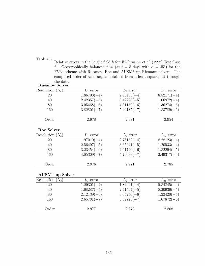
Table 4.3:Relative errors in the height field h for Williamson et al. (1992) Test Case2 – Geostrophically balanced flow (at t = 5 days with α = 45) for theFV3s scheme with Rusanov, Roe and AUSM+-up Riemann solvers. Thecomputed order of accuracy is obtained from a least squares fit throughthe data.

Rusanov SolverResolution (Nc) L1 error L2 error L∞ error

20 1.86793(−4) 2.65483(−4) 8.52171(−4)40 2.42357(−5) 3.42298(−5) 1.06972(−4)80 3.05468(−6) 4.31159(−6) 1.36274(−5)160 3.82801(−7) 5.40185(−7) 1.83789(−6)

Order 2.978 2.981 2.954

Roe SolverResolution (Nc) L1 error L2 error L∞ error

20 1.97019(−4) 2.78152(−4) 8.28123(−4)40 2.56497(−5) 3.65241(−5) 1.20533(−4)80 3.23454(−6) 4.61740(−6) 1.82294(−5)160 4.05309(−7) 5.79033(−7) 2.49317(−6)

Order 2.976 2.971 2.785

AUSM+-up SolverResolution (Nc) L1 error L2 error L∞ error

20 1.29301(−4) 1.84921(−4) 5.84845(−4)40 1.68287(−5) 2.41594(−5) 8.20936(−5)80 2.12139(−6) 3.05250(−6) 1.22420(−5)160 2.65731(−7) 3.82725(−7) 1.67872(−6)

Order 2.977 2.973 2.808

136

Table 4.4: As Table 4.3 except with the FV4 scheme.Rusanov Solver

Resolution (Nc) L1 error L2 error L∞ error20 1.23147(−5) 1.83684(−5) 5.28083(−5)40 3.92605(−7) 6.14237(−7) 3.30766(−6)80 1.42768(−8) 2.19348(−8) 1.94550(−7)160 6.44784(−10) 9.23157(−10) 1.09139(−8)

Order 4.744 4.765 4.081

Roe SolverResolution (Nc) L1 error L2 error L∞ error

20 3.33670(−6) 4.71855(−6) 1.33113(−5)40 1.56059(−7) 2.14543(−7) 5.63099(−7)80 8.67290(−9) 1.17659(−8) 2.79641(−8)160 5.19851(−10) 7.03778(−10) 1.62477(−9)

Order 4.211 4.232 4.333

AUSM+-up SolverResolution (Nc) L1 error L2 error L∞ error

20 3.26183(−6) 4.66310(−6) 1.19600(−5)40 1.54530(−7) 2.14661(−7) 5.14470(−7)80 8.65658(−9) 1.18352(−8) 2.70597(−8)160 5.19867(−10) 7.06975(−10) 1.64234(−9)

Order 4.200 4.224 4.274

137

Figure 4.9:As Figure 4.8 except using the FV4 scheme. Contour lines are in units of5× 10−4m.

The details of the rotated coordinate system are described in Williamson et al. (1992).

The analytic height field is given by

h = h0 −1

G

θ′∫−π/2

(2Ω sin τ + u′λ(τ) tan τ)u′λ(τ)dτ, (4.97)

which must be integrated numerically at each point where h is desired. The back-

ground height and velocity fields are again chosen to be

h0 = 4.7057× 10−4 Earth radii, and u0 =π

6Earth radii/day. (4.98)

Further, the compact height field is determined by the parameters

θb = −π6, θe =

π

2, and xe = 0.3. (4.99)

138

This test case again represents an unstable equilibrium solution to the shallow-water

equations, and so is not preserved in the long-term in most atmospheric models. We

again use high-order Gaussian quadrature to initialize the height and momentum

fields in the numerical model and run the model for five days. In all cases we make

use of a rotation angle of 60. The timestep at 40× 40× 6 resolution for this case is

∆t = 17.5 minutes.

The results of the convergence study for the two schemes with all Riemann solvers

is given in Tables 4.5 and 4.6. Again we see similar convergence rates to that of test

case 2, except noting that we see a significant gain in accuracy (a 3× improvement

in the L1 norm) when going from the Rusanov Riemann solver to either the Roe

or AUSM+-up Riemann solver. For the FV3s scheme we observe slightly better

performance from the Roe solver over AUSM+-up, and the opposite for the FV4

scheme.

Error plots are given in Figures 4.10 and 4.11. The error plots from the Roe and

AUSM+-up Riemann solvers are very similar, as expected given their similar error

norms. However, we see very strong error due to diffusivity in the results from the

Rusanov scheme of almost an order of magnitude more than the other two approaches.

4.7.4 Zonal Flow over an Isolated Mountain

Test case 5 in Williamson et al. (1992) considers flow with a topographically driven

source term. The wind and height fields are defined as in section 4.7.2, except with

α = 0, h0 = 5960 m and u0 = 20 m/s. A conical mountain is introduced into the

flow, given by

z = z0(1− r/R), (4.100)

with z0 = 2000 m, R = π/9 and r2 = min [R2, (λ− λc)2 + (θ − θc)2]. The center of

the mountain is taken as λc = 3π/2 and θc = π/6.

We plot the height field at day 5, 10 and 15 in Figure 4.12 on a 40× 40× 6 grid

139

Figure 4.10:Background height field (top-left, in m) and absolute errors associatedwith the FV3s scheme on a 40 × 40 × 6 grid with Rusanov (top-right),Roe (bottom-left) and AUSM+-up (bottom-right) Riemann solvers forWilliamson et al. (1992) test case 3 with α = 60. Contour lines arein units of 10−1 m, with solid lines corresponding to positive values anddashed lines corresponding to negative values. The thick line correspondsto zero error.

140

Table 4.5:Relative errors in the height field h for Williamson et al. (1992) Test Case3 – Geostrophically balanced flow with compact support (at t = 5 dayswith α = 60) for the FV3s scheme with Rusanov, Roe and AUSM+-upRiemann solvers. The computed order of accuracy is obtained from a leastsquares fit through the data.

Rusanov SolverResolution (Nc) L1 error L2 error L∞ error

20 5.29489(−4) 1.04318(−3) 6.98472(−3)40 4.14616(−5) 7.62192(−5) 4.36449(−4)80 4.90936(−6) 8.83443(−6) 4.42438(−5)160 6.24068(−7) 1.11900(−6) 5.91343(−6)

Order 3.226 3.270 3.392

Roe SolverResolution (Nc) L1 error L2 error L∞ error

20 1.72217(−4) 3.13719(−4) 1.60254(−3)40 1.79322(−5) 3.39544(−5) 1.93667(−4)80 2.41481(−6) 4.62184(−6) 2.70813(−5)160 3.09483(−7) 5.94444(−7) 3.46030(−6)

Order 3.025 3.001 2.940

AUSM+-up SolverResolution (Nc) L1 error L2 error L∞ error

20 1.47699(−4) 2.71802(−4) 1.26574(−3)40 1.89854(−5) 3.69259(−5) 2.24091(−4)80 2.61576(−6) 5.16111(−6) 3.13437(−5)160 3.36013(−7) 6.64243(−7) 4.00544(−6)

Order 2.920 2.887 2.775

141

Table 4.6: As Table 4.5 except with the FV4 scheme.Rusanov Solver

Resolution (Nc) L1 error L2 error L∞ error20 3.95805(−4) 7.38801(−4) 4.44070(−3)40 1.65282(−5) 3.13826(−5) 1.89074(−4)80 5.41290(−7) 1.02393(−6) 5.96072(−6)160 1.70040(−8) 3.19845(−8) 1.79530(−7)

Order 4.845 4.842 4.877

Roe SolverResolution (Nc) L1 error L2 error L∞ error

20 1.22144(−4) 2.35850(−4) 1.28707(−3)40 4.48290(−6) 8.67097(−6) 4.67861(−5)80 1.50958(−7) 2.89663(−7) 1.50027(−6)160 5.49471(−9) 1.04223(−8) 5.04890(−8)

Order 4.821 4.830 4.888

AUSM+-up SolverResolution (Nc) L1 error L2 error L∞ error

20 1.01946(−4) 2.01244(−4) 1.22075(−3)40 3.76651(−6) 7.45425(−6) 4.44324(−5)80 1.29063(−7) 2.53563(−7) 1.44834(−6)160 4.93269(−9) 9.55944(−9) 4.99077(−8)

Order 4.787 4.796 4.867

142

Figure 4.11:As Figure 4.10 except using the FV4 scheme. Contour lines are in unitsof 3× 10−2m.

with a timestep of 12.5 minutes.

Potential enstrophy ξ and total energy E are invariant under the shallow-water

equations, and are defined by

ξ =(ζ + f)2

2h, and E = 1

2hv · v + 1

2G(H2 − z2). (4.101)

From the element-averages of the height and momentum field, we calculate total

energy directly, weighting element-wise totals by element area. Similarly, potential

enstrophy is calculated by using a central-difference approximation to the curl and

then using element-averages. The resulting computed invariants are accurate up to

O(∆2).

We compare our results with the reference solution of Jakob-Chien et al. (1995),

which is run on the spectral transform shallow-water model (STSWM) at T426 reso-

143

lution. This high resolution reference solution was computed by the German Weather

Service (DWD) and is available online (http://icon.enes.org/swm/stswm/node5.html).

The T426 simulation utilized a Gaussian grid with 640 × 1280 grid points in latitu-

dinal and longitudinal direction which corresponds to a grid spacing of about 31 km

at the equator. To directly compare with our model, the spectral coefficients from

STSWM are sampled on the cubed-sphere grid at high-resolution Gaussian quadra-

ture points in order to obtain element-averages of the state variables on a 40× 40× 6

grid. Invariants are then calculated from the resampled cubed-sphere solution and

our own cubed-sphere runs using standard difference operators.

The normalized total potential enstrophy and total energy difference from the

initial state versus time are given for the FV3s scheme in Figure 4.13 and for the

FV4 scheme in Figure 4.14. We observe very good performance of both schemes with

respect to conservation of these quantities, with the best conservation properties

coming from the AUSM+-up Riemann solver (the Roe Riemann solver also matches

very closely). The Rusanov Riemann solver performs significantly worse in all cases,

due to the significant diffusion in this scheme.

4.7.5 Rossby-Haurwitz Wave

The Rossby-Haurwitz wave (test case 6 in Williamson et al. (1992)) is an analytic

solution of the nonlinear barotropic vorticity equation on the sphere. The height and

velocity field can be analytically computed with several free parameters, however for

the purposes of testing the numerical model we only make use of the wave number

4 test. Our parameters are analogous to those of Williamson et al. (1992), who also

provides expressions for the analytic fields for this test case. Again, we make use of

high-order Gaussian quadrature to calculate the initial height and momentum fields.

It is well known that the wave number 4 Rossby-Haurwitz wave is susceptible to

instability which can be driven by truncation error in the initial conditions (see, for

144

Figure 4.12:Total height field for Williamson et al. (1992) test case 5. We show thesimulation results for the FV4 scheme with AUSM+-up Riemann solversimulated on a 40×40×6 grid. The dashed circle represents the locationof the conical mountain. Contour levels are from 4950 m to 5950 m inintervals of 50 m, with the highest elevation being near the equator (thesmall enclosed contours). The results for the FV3s scheme are visuallyidentical.

145

Figure 4.13:Normalized potential enstrophy (top) and total energy (bottom) differ-ence for the flow over an isolated mountain test case using the FV3sscheme simulated on a 40× 40× 6 grid.

146

Figure 4.14:Normalized potential enstrophy (top) and total energy (bottom) differ-ence for the flow over an isolated mountain test case using the FV4scheme simulated on a 40× 40× 6 grid.

147

example, Thuburn and Li (2000)), and hence will eventually collapse into a turbulent

flow. The time of the breakdown varies based on the numerical scheme employed and

the choice of grid resolution. For the FV3s and FV4 schemes discussed in this chapter,

we begin to see breakdown at about day 80, but find that adding perturbations on

the order of the scheme’s truncation error can drive the collapse to as early as day

30.

We plot the height field for the FV3s scheme in Figure 4.15 and for the FV4

scheme in Figure 4.16 at day 0, 7, 14, 30, 60 and 90 at a resolution of 80×80×6. The

higher resolution is required for the plots to capture some of the small scale features

of the wave profile. The total energy and potential enstrophy computed at each day

of the simulation (up to day 14) is presented in Figures 4.17 and 4.18, compared

against the STSWM reference solution at T511 (26 km) resolution truncated to the

cubed-sphere at 40× 40× 6 for consistency with Figures 4.13–4.14. The timestep is

chosen to be 4.2 minutes for the 80× 80× 6 runs and 8.4 minutes for the 40× 40× 6

runs. Again, the Roe and AUSM+-up Riemann solvers perform very well, whereas

the Rusanov Riemann solver performs noticably worse. The finite-volume nature of

the underlying scheme imposes fairly strong diffusivity on the energy when compared

to the reference solution, but nonetheless we observe similar conservation properties

to competing schemes.

4.7.6 Barotropic Instability

The barotropic instability test case of Galewsky et al. (2004) consists of a zonal

jet with compact support at a latitude of 45. A small height disturbance is added

which causes the jet to become unstable and collapse into a highly vortical structure.

The relative vorticity is used here as a comparison between the solution presented in

Galewsky et al. (2004) (obtained via a spectral transform method) and the solution

obtained by direct simulation. We present the potential vorticity at varying resolu-

148

Figure 4.15:Wavenumber four Rossby-Haurwitz wave (test case 6 in Williamson et al.(1992)). The solution is computed on a 80× 80× 6 grid using the FV3sscheme with AUSM+-up solver on day 0, 7 and 14 (left column, from topto bottom) and day 30, 60 and 90 (right column, from top to bottom).The contour levels are from 8100 m to 10500 m in increments of 100 m,with the innermost contours being the highest.

149

Figure 4.16: As Figure 4.15 except for the FV4 scheme.

150

Figure 4.17:Normalized potential enstrophy (top) and potential energy (bottom) dif-ference for the Rossby-Haurwitz wave test case using the FV3s methodsimulated on a 40× 40× 6 grid.

151

Figure 4.18:Normalized potential enstrophy (top) and potential energy (bottom) dif-ference for the Rossby-Haurwitz wave test case using the FV4 simulatedon a 40× 40× 6 grid.

152

tions for the FV3s and FV4 scheme with AUSM+-up Riemann solver in Figures 4.19

and 4.20, respectively. The timestep used for this test case is 9 minutes at a resolution

of 40× 40× 6. No artificial viscosity is added in our simulation, since the numerical

diffusion introduced by the finite-volume method is sufficient to ensure stability.

As observed by St-Cyr et al. (2008), this test case is particularly difficult for models

using the cubed-sphere to handle. Since the jet passes over cubed-sphere panel edges

eight times and is driven by a relatively mild perturbation, wave number four grid

forcing is significant in disturbing the collapse for resolutions less than approximately

100×100×6. For higher resolutions however, we observe convergence to the reference

solution given by Galewsky et al. (2004) and similarity to the solution calculated by

Rossmanith (2006) (except without the need to split the geostrophically balanced and

unsteady modes).

4.7.7 Computational Performance

The utility of any computational scheme is a function of both accuracy and com-

putational performance. Hence, we present the relative cost of the third- and fourth-

order schemes (along with each choice of Riemann solver) in Table 4.7. As expected,

we see an overall increase in cost with increasing complexity of the Riemann solver,

as well as a much more significant jump in computational cost associated with going

from the third- to fourth-order scheme. As is usual for explicit methods, a doubling

of the resolution will lead to an eight times increase in the computational time for

the scheme when keeping the CFL number constant.

Considering the significant improvement in accuracy we have observed from using

the Roe or AUSM+-up Riemann solvers, the added expense they incur in computation

time is negligible.

153

Figure 4.19:Relative vorticity field associated with the barotropic instability testat day 6 obtained from the FV3s scheme with AUSM+-up solver on a40× 40× 6 mesh (top), 80× 80× 6 mesh (2nd from top), 120× 120× 6mesh (3rd from top) and 160×160×6 mesh (bottom). Contour lines arein increments of 2.0 × 10−5s−1 from −1.1 × 10−4s−1 to −0.1 × 10−4s−1

(dashed) and from 0.1× 10−4s−1 to 1.5× 10−4s−1 (solid). The zero lineis omitted. Only the northern hemisphere is depicted in this plot.

154

Figure 4.20: As Figure 4.19 except for the FV4 scheme.

155

Table 4.7:The approximate computational performance for each of the numericalschemes paired with each Riemann solver, as obtained from serial runs ona MacBook Pro with 2.4 GHz Intel Core 2 Duo. The timings correspondto the number of seconds required to simulate one day of Williamson testcase 2 (described in Section 4.7.2) on a 40× 40× 6 grid. A CFL numberof 1.0 is used in all cases.

Scheme Rusanov Roe AUSM+-upFV3s 10.0 s 10.6 s 10.9 sFV4 23.8 s 24.5 s 25.0 s

4.8 Conclusions and Future Work

In this chapter, we have successfully demonstrated both a dimension-split piece-

wise parabolic scheme and a fourth-order accurate piecewise cubic method for solving

the shallow-water equations on the sphere. We have applied both of these schemes to

a set of test problems in order to verify accuracy, stability and convergence, including

the shallow-water test cases of Williamson et al. (1992) and the barotropic instabil-

ity of Galewsky et al. (2004). Third- and fourth-order accuracy of these schemes is

apparent in the smooth simulations tested in this chapter.

Three Riemann solvers have been considered in this analysis, including the Ru-

sanov numerical flux, the Roe solver of Roe (1981), and the AUSM+-up numerical

flux of Liou (2006). Our simulations have shown that the AUSM+-up flux provides

the best overall accuracy when applied to various shallow-water test cases, followed

very closely by the Roe flux. The Rusanov solver has demonstrated significantly

worse performance in terms of accuracy and conservation of flow invariants, which

we believe outweighs its simplicity. Importantly, the overall improvement in accuracy

due to the Roe or AUSM+-up solvers has been shown to come without a significant

added computational expense.

Extension of the work described herein to a full 3D atmospheric model certainly

deserves some attention. Adaption of the Riemann solvers to the full Euler equations

is a trivial task, but one must be careful in the reconstruction step and in making a

156

choice of the timestepping method. The choice of reconstruction is dependent on the

vertical coordinate system, of which there are three possible routes forward: First,

the high-order FV approach discussed herein is perhaps most directly applied with a

semi-Lagrangian vertical coordinate, such as that described by Lin (2004). Second,

a static terrain-following coordinate could be adopted (see, for instance, Kasahara

(1974); Phillips (1957); Wood and Staniforth (2003)). Finally, a static height-based

coordinate could be used, with topography incorporated via partial-shaved cells (see,

for example, Adcroft et al. (1997); Black (1994)). For the first two choices of vertical

coordinate, it is unknown what effect the vertically non-Cartesian geometry will have

on the accuracy of the reconstruction step. Analysis of these approaches represents

ongoing research. The second two choices of vertical coordinate also introduce issues

with regard to the choice of a vertical timestepping scheme, since atmospheric models

must incorporate horizontal/vertical aspect ratios that are sometimes on the order of

∼ 103. In this case, the vertical CFL condition tends to be unmanagably restrictive.

To overcome this problem, one could either use a modified equation set that removes

vertically-propagating soundwaves (see, for example, Arakawa and Konor (2009);

Davies et al. (2003)) or use a dimension-split implicit-explicit integrator (such as

the IMEX-RK scheme of Ascher et al. (1997)). Other methods include semi-implicit

treatment of sound waves or a split-explicit approach with subcycling. Research is

ongoing as to the best route forward.

Acknowledgements

We would like to thank Dr. Meng-Sing Liou for his assistance with fine-tuning

the AUSM+-up solver for unstable shallow-water flow and Dr. Smadar Karni for her

assistance with the topography parameterization. This work was supported by the

NSF Collaboration in Mathematical Geosciences (CMG) grant ATM-0723440.

157

This work can be found in Ullrich et al. (2010).

158

CHAPTER V

Operator-Split Runge-Kutta-Rosenbrock (RKR)

Methods for Non-hydrostatic Atmospheric Models

5.1 Introduction

One reason explicit time-stepping schemes are desirable in atmospheric models is

locality of data, which allows the equations of motion to be evaluated with minimal

communication between neighboring elements. In the context of large-scale parallel

systems this benefit means that communication between processors is significantly

less than with equivalent implicit methods. Nonetheless, purely explicit methods

have strict time step restrictions that are required for stability. The fast moving

waves in the governing equation largely determine this time step restriction, although

they may possess little physical significance. In general, the maximum stable time

step for explicit time discretizations is determined by the dimensionless Courant-

Friedrichs-Lewy (CFL) number, which takes the form

ν =cmax∆t

∆x, (5.1)

where cmax denotes the maximum wave speed of the system, ∆x is the minimum

grid spacing and ∆t is the maximum stable time step. Most explicit time stepping

methods are limited to ν . 1. In atmospheric flows, sound waves are the fastest

159

propagating wave modes, with an average speed of 340 m s−1 at sea level. At ∆x ≈

110 km resolution (which corresponds to about a 1 grid spacing at the equator),

this leads to a time step restriction of about five minutes. Contrasting this against a

vertical discretization with a minimum near-surface grid spacing of about 100 m, the

maximum time step restriction is merely ∆t . 0.3 seconds – 1000 times smaller than

the horizontal time step. With our current computing power, atmospheric modeling

would be effectively impossible at such a time step.

Various methods have been developed to deal with the computational restrictions

introduced by fast waves in the atmosphere. The first method arises from a mod-

ification of the equation set to “filter” out fast-moving waves. At large horizontal

scales, hydrostatic models (including Taylor et al. (2008) and Lin (2004)) are usually

employed to remove the acceleration of the vertical velocity from the system. This

approach eliminates vertically-propagating sound waves, but reaches its limitations

when the grid size is reduced to “non-hydrostatic” scales around 10 km. Motions at

this scale can be dominated by large vertical velocities, and so the vertical acceler-

ation term cannot be neglected. Further, the dispersion relation of the hydrostatic

equation set reveals that the phase speed of gravity-wave modes can be overestimated

at these scales, as compared to the full non-hydrostatic equations (Durran, 1999). Al-

ternatively, “sound-proof” systems of equations, including the Boussinesq equations,

the anelastic system of Ogura and Phillips (1962), the pseudo-incompressible system

of Durran (1989) and the unified approximation of Arakawa and Konor (2009), have

been successfully used in models by removing sound waves from the governing equa-

tions. Nonetheless, one must be aware that these modified systems may not be valid

on all scales, and therefore may not be desirable for global atmospheric models (see,

for example, Davies et al. (2003)).

The second method for dealing with computationally fast waves relies on numer-

ical methods which treat these modes in a stable manner. In particular, we focus on

160

methods which integrate the full non-hydrostatic equation set, but introduce a split-

ting strategy to deal with fast wave modes. These approaches are generally referred

to as “operator-split methods.” Operator-split methods have been in use for atmo-

spheric models for quite some time, beginning with the first semi-implicit methods

of Kwizak and Robert (1971). Since then, semi-implicit methods have been used in

atmospheric models at practically all scales (see, for example, Bonaventura (2000);

Thomas and Loft (2002); Restelli and Giraldo (2009)). Closely related to semi-implicit

methods are split-explicit and fractional step techniques. These methods are simi-

lar but instead combine explicit operators, generally splitting on the slow and fast

waves. These methods were originally developed by Gadd (1978) for atmospheric

models, but they continue to be in use today. The Weather Research and Forecasting

Model (WRF, Skamarock and Klemp (2008)), for example, uses both semi-implicit

and explicit splitting, utilizing implicit integration for vertically propagating waves

and a split-explicit technique for fast waves in the horizontal.

In this chapter we introduce a new time discretization for models that split the

temporal and spatial derivatives using the method of lines. The proposed method

offers a simple framework for achieving high-order temporal accuracy in a semi-

implicit scheme while maintaining computational efficiency. Following an operator-

split Runge-Kutta-Rosenbrock (RKR) strategy, which combines an explicit Runge-

Kutta (RK) method with a linearly implicit Rosenbrock step (Rosenbrock , 1963),

we obtain a method whose maximum stable time step is constrained only by the

horizontal CFL number. To maximize efficiency on parallel systems, the splitting is

performed on the horizontal and vertical components of the governing equations so

that the implicit solve is a local operation. This strategy is demonstrated using a

high-order finite-volume method in 2D and 3D so as to verify accuracy and stability,

but this approach is easily extended to other methods which independently discretize

space and time, such as discontinuous Galerkin. The approach presented herein is

161

valid for all horizontal scales, and hence may be especially well-suited for models that

utilize adaptively refined meshes with scale differences.

In section 5.2 we introduce the full non-hydrostatic fluid equations and explain how

to incorporate terrain-following coordinates. The RKR discretization is introduced

in section 5.3, wherein we present a first-order, a second-order and a third-order

temporal discretization that is stable for high-order spatial discretizations. We will

demonstrate these techniques using high-order finite-volume spatial discretizations,

which are explained in section 5.4, followed by numerical results in section 5.5. Our

conclusions are given in section 5.6.

5.2 The non-hydrostatic fluid equations in Cartesian coordi-

nates

We utilize the shallow-atmosphere non-hydrostatic fluid equations written in terms

of the conservative variables density ρ, momentum ρu (where u is the 3D velocity

vector) and potential temperature density ρθ. In vector form, these equations are

written as follows:

∂ρ

∂t+∇ · (ρu) = 0, (5.2)

∂ρu

∂t+∇ · (ρu⊗ u + pI) = −ρgez − fez × (ρu), (5.3)

∂ρθ

∂t+∇ · (ρθu) = 0. (5.4)

Here ⊗ denotes the tensor (outer) product, I denotes the identity matrix, ez is the

basis vector in the z direction, g is gravity and f is the Coriolis parameter. A list

of the constants used in this chapter and their corresponding values can be found

in Table 5.1. The pressure p in the momentum equation is related to the potential

162

Table 5.1: List of parameters and physical constants used in this chapter.

Parameter Description Control Valuea Radius of the Earth 6.37122× 106 mΩ Rotational speed of the Earth 7.292 × 10−5 s−1

g Gravity 9.80616 m s−2

p0 Background surface pressure 1000 hPacp Specific heat capacity of dry air at constant pressure 1004.5 J kg−1 K−1

cv Specific heat capacity of dry air at constant volume 717.5 J kg−1 K−1

Rd Ideal gas constant of dry air 287.0 J kg−1 K−1

temperature density via the equation of state

p = p0

(Rd(ρθ)

p0

)cp/cv. (5.5)

The second terms on the left-hand-side of (5.2)-(5.4) are referred to as flux terms,

since they determine the flow rate of the conservative state variables through the

edges of a spatial region. The terms on the right-hand-side of these equations are

source terms. Nonhydrostatic mesoscale models that use a closely related equation

set include the WRF model (see, for example, Skamarock and Klemp (2008)) and the

model by Ahmad and Lindeman (2007).

A splitting is performed on these equations of the form

ρ(x, t) = ρ(x) + ρ′(x, t), (5.6)

p(x, t) = p(x) + p′(x, t), (5.7)

(ρθ)(x, t) = ρθ(x) + (ρθ)′(x, t), (5.8)

where the mean values (denoted by the overbar) are in local hydrostatic balance, i.e.

∂p

∂z= −ρg, (5.9)

163

and satisfy (5.5). This choice is required to remove errors in approximating the

hydrostatic state of the atmosphere that could be responsible for significant generation

of spurious vertical momentum.

5.2.1 Incorporating topography

For the time stepping schemes presented in this chapter, we will be using terrain-

following coordinates as introduced by Gal-Chen and Somerville (1975). A possible

alternative to terrain-following coordinates are so-called shaved-cell methods (see,

for example, Adcroft et al. (1997)), which remove the portions of a cell occupied by

topography. Unfortunately, if terrain is accurately resolved, this approach will reduce

the horizontal extent of an element, and hence the maximum allowable horizontal

time step. Modified shaved-cells that do not reduce the horizontal extent of cells

could also be used, but this technique may significantly degrade the accuracy of the

terrain discretization.

Under an arbitrary change-of-coordinates, the non-hydrostatic governing equa-

tions (5.2)-(5.4) take the form

∂ρ

∂t+

1

J∇j(Jρu

j) = 0, (5.10)

∂ρui

∂t+

1

J∇j(J(ρuiuj + pGij)) = Γijk(ρu

juk + pGjk) + ψig + ψic, (5.11)

∂ρθ

∂t+

1

J∇j(Jρθu

j) = 0, (5.12)

where we have chosen to use Einstein summation notation to denote vector compo-

nents. Here Gij denotes the contravariant metric with covariant inverse Gij = (Gij)−1,

J = det(Gij) is the volume-element and Γijk denotes the Christoffel symbols of the

second kind, given below. The momentum equation source terms due to gravity and

Coriolis are ψig and ψic, respectively.

Here we define regional terrain-following coordinates (X, Y, Z) over some oro-

164

graphic field h = h(x, y) in terms of their Cartesian counterparts via

X = x, Y = y, Z = H

(z − hH − h

). (5.13)

Here H denotes the model height, at which point the terrain-following coordinates

and Cartesian coordinates are identical (Z = z). The basis vectors (eX , eY , eZ) are

related to the Cartesian basis vectors (ex, ey, ez) via

eX = ex +

(∂h

∂x

)(1− Z

H

)ez, (5.14)

eY = ey +

(∂h

∂y

)(1− Z

H

)ez, (5.15)

eZ =

(1− h

H

)ez. (5.16)

These relations can be inverted to obtain the Cartesian basis vectors in terms of

terrain-following coordinates, as required for computing the gravitational and Coriolis

forcing:

ex = eX −(∂h

∂x

)(H − ZH − h

)eZ , (5.17)

ey = eY −(∂h

∂y

)(H − ZH − h

)eZ , (5.18)

ez =

(H

H − h

)eZ . (5.19)

The contravariant metric for this choice of coordinates (again, see Gal-Chen and

Somerville (1975)) is

Gij =

1 0 − (H − Z)

(H − h)

(∂h

∂x

)0 1 − (H − Z)

(H − h)

(∂h

∂y

)− (H − Z)

(H − h)

(∂h

∂x

)− (H − Z)

(H − h)

(∂h

∂y

) (H

H − h

)2

+

(H − ZH − h

)2[(

∂h

∂x

)2

+

(∂h

∂y

)2]

,

(5.20)

165

with metric determinant

J = 1− h

H. (5.21)

This leads to Christoffel symbols

ΓXjk = 0, ΓY

jk = 0, ΓZjk =

(H − Z)

(H − h)

(∂2h

∂x2

)(H − Z)

(H − h)

(∂2h

∂x∂y

)− 1

(H − h)

(∂h

∂x

)(H − Z)

(H − h)

(∂2h

∂x∂y

)(H − Z)

(H − h)

(∂2h

∂x2

)− 1

(H − h)

(∂h

∂y

)− 1

(H − h)

(∂h

∂x

)− 1

(H − h)

(∂h

∂y

)0

.

(5.22)

Under this choice of coordinates, the source terms take the form

ψXg = 0, ψYg = 0, ψZg = −ρg H

H − h, (5.23)

and

ψXc = fρuY , ψYc = −fρuX , ψZc = f

(z −HH − h

)[(∂h

∂x

)(ρuY )−

(∂h

∂y

)(ρuX)

].

(5.24)

5.3 Runge-Kutta-Rosenbrock (RKR) Schemes

The method of lines approach is one of the most popular methods for constructing

high-order finite-volume methods that are applicable to general systems of partial

differential equations (PDEs). Under this framework the spatial terms, including the

flux and source terms, are discretized first, leading to a system of ordinary differential

equations (ODEs) for the state variables within each grid cell. This system is then

discretized by means of choosing an appropriate time stepping scheme. The time

stepping scheme must be chosen so that the eigenvalues of the spatial operator fit

within the scheme’s stability region. Explicit schemes are generally computationally

inexpensive, but possess a restricted stability region, whereas implicit schemes are

166

more costly, but possess a large stability region. However, different physical processes

can have eigenvalues that have dramatically different structure, and so it may not be

appropriate to use a single time-stepping method to integrate all terms of the ODE

system.

5.3.1 The Runge-Kutta-Rosenbrock approach

Implicit-explicit (IMEX) methods represent a category of general-purpose schemes

for ODEs that couple implicit and explicit time integration methods. These meth-

ods have been in use as early as the 1970s (for example, Crouzeix (1980) and Varah

(1980)). More recently, a family of implicit-explicit Runge-Kutta (IMEX-RK) schemes

was collected into a general framework by Ascher et al. (1997) in their seminal paper.

They showed that it is possible to achieve an essentially arbitrary order-of-accuracy

by correctly interleaving explicit and implicit steps, although with increasing compu-

tational expense.

IMEX methods are usually applied to an ODE of the form

∂q

∂t= f(q) + g(q), (5.25)

where q is some state vector. In particular, we assume that the terms f(q) are not stiff;

mathematically, one can think of this as saying that the eigenvalues of the operator

f are close to the origin. On the other hand, the terms grouped under the g(q)

operator are assumed stiff, containing eigenvalues which are potentially unbounded.

This stiffness can originate from short time-scale behavior, such as chemistry or, as

in our case, from geometric stiffness due to a discrepancy in grid spacing in different

coordinate directions. Since we focus on the dynamical aspects of the atmosphere,

f(q) is assumed to be some horizontal spatial discretization of the fluid equations with

grid spacing ∆x and g(q) is a vertical discretization with grid spacing ∆z ∆x.

167

The much smaller vertical scale leads to eigenvalues of g that are typically far from

the origin. Herein, we will see that the terms f(q) and g(q) arise naturally out of

some spatial discretization of the non-hydrostatic model equations (5.2)-(5.5).

To improve the performance of the IMEX methods we focus on the family of

operator-split RKR methods, which are identical to IMEX schemes except replacing

the computationally expensive implicit step with a so-called Rosenbrock step. Rosen-

brock methods were originally developed by Rosenbrock (1963) in the 1960s and later

refined by Nørsett and Wolfbrandt (1979). More recently, a framework for high-order

RKR time stepping methods has been presented by Jebens et al. (2010) for use in

atmospheric models utilizing cut-cells.

In an implicit approach, one usually ends up with a nonlinear system of equations

of the form

F(x) = 0 (5.26)

that must be solved numerically for some vector x. Perhaps the most well-known and

robust technique for solving this system is the Newton-Krylov algorithm, which is an

iterative approach defined by

x(i) = x(i−1) −[dF

dx

∣∣∣∣x=x(i−1)

]−1

F(x(i−1)). (5.27)

When applied to systems of ODEs obtained from time-split PDE systems, the Newton-

Krylov method is usually initialized by taking x(0) to be the value of x obtained at

the previous time step. Although this method converges quadratically, the Jacobian

dF/dx must nonetheless be computed (numerically or analytically) at every itera-

tion. Under the Rosenbrock method, one does not require nonlinear convergence of

(5.26), and instead only takes one step of (5.27). This significantly reduces the costs

associated with the implicit step and restricts the number of Jacobian evaluations to

one per Rosenbrock step.

168

In order to obtain high-order-accuracy in time with our scheme, we consider a gen-

eral Runge-Kutta method with interleaved explicit and linearly implicit Rosenbrock

steps. In the general RKR framework, we define the initial data by

q(0) = qn, (5.28)

and then each subsequent step by

q(i) =i−1∑k=0

αi,kq(k) + Eiβi∆tf(q(i−1)) + (1− Ei)βi∆t

(I + βi∆tDg(q(i−1))

)−1g(q(i−1)),

(5.29)

where αi,k and βi are arbitrary coefficients, ∆t is the time step, Dg denotes the

Jacobian of g, and E is a binary indicator variable,

Ei =

1, for an explicit step,

0, for a Rosenbrock step.(5.30)

This scheme description is interchangeable with the dual Butcher-tableau approach

of Ascher et al. (1997), but is preferred in this chapter since it is more closely linked

with the method’s actual implementation.

5.3.2 A crude splitting scheme

Perhaps the simplest stable scheme for splitting the explicit and linearly implicit

components of the evolution equations involves simply applying a high-order explicit

Runge-Kutta operator to the explicit terms followed by the Rosenbrock operator

applied at the full time step. If we use the third-order strong-stability-preserving

(SSP) RK3 scheme of Gottlieb et al. (2001) for the explicit component, this scheme

169

proceeds according to

q(1) = qn + ∆tf(qn), (5.31)

q(2) =3

4q(1) +

1

4q(1) +

∆t

4f(q(1)), (5.32)

q(3) =1

3qn +

2

3q(2) +

2∆t

3f(q(2)), (5.33)

qn+1 ≡ q(4) = q(3) + ∆t(I−∆tDg(q(3))

)−1g(q(3)) (5.34)

Here the indices n and n+ 1 denote the current and future time step. This scheme is

first-order accurate in time and extremely diffusive (as demonstrated in section 5.5.1).

As a consequence, we do not recommend using this scheme in practice.

5.3.3 The second-order-accurate Strang-Carryover scheme

To achieve second-order accuracy in time, we suggest a splitting scheme pointed

out by Steve Ruuth (2010, personal communication) and based on Strang splitting

of the explicit and implicit operators. This scheme combines a third-order SSP RK3

step with one implicit solve per time step. However, at the first time step, we must

perform one additional implicit operation, storing

G0 =

(I− ∆t

2Dg(q0)

)−1

g(q0). (5.35)

170

After this initialization step, the algorithm proceeds as follows:

q(1) = qn +∆t

2Gn, (5.36)

q(2) = q(1) + ∆tf(q(1)), (5.37)

q(3) =3

4q(1) +

1

4q(2) +

∆t

4f(q(2)), (5.38)

q(4) =1

3q(1) +

2

3q(3) +

2∆t

3f(q(3)), (5.39)

Gn+1 =

(I− ∆t

2Dg(q(4))

)−1

g(q(4)), (5.40)

qn+1 = q(4) +∆t

2Gn+1. (5.41)

This scheme can achieve third-order linear and nonlinear accuracy in f plus second-

order accuracy in g.

5.3.4 The Ascher-Ruuth-Spiteri (2,3,3) scheme

A third-order operator-split RKR scheme can be obtained from the Ascher-Ruuth-

Spiteri (2,3,3) scheme of Ascher et al. (1997), hereafter referred to as the ARS(2,3,3)

scheme. If we simply replace the implicit solve with a Rosenbrock step, the resulting

scheme takes the form

q(1) = qn + γc∆tf(qn), (5.42)

q(2) = q(1) + γc∆t(I− γc∆tDg(q(1))

)−1g(q(1)), (5.43)

q(3) =1

γcqn +

(3γc − 2)

γcq(1) +

(1− 2γc)

γcq(2) + 2(1− γc)∆tf(q(2)), (5.44)

q(4) = q(3) + γc∆t(I− γc∆tDg(q(3))

)−1g(q(3)), (5.45)

qn+1 = −1

2qn − 3γc

2q(1) +

3

2q(2) +

3(3γc − 2)

2q(3) +

1

2γcq(4) +

∆t

2f(q(4)),(5.46)

where

γc =3 +√

3

6. (5.47)

171

This scheme is linearly third-order accurate in both f , g and any cross-terms that

arise from the integration procedure, but is only nonlinearly third-order accurate in

f . In fact, when g = 0 the stability region for this scheme is exactly the stabil-

ity region of the usual three-stage third-order-accurate Runge-Kutta operator. This

scheme requires three explicit steps per time step and two Rosenbrock steps, with

each Rosenbrock step consisting of a single evaluation of the Jacobian and a sin-

gle linear solve. As a consequence, the overall computational cost of this method is

approximately twice that of the Strang-carryover scheme.

5.4 Spatial discretization

In this section we turn our attention to the spatial discretization of the 3D non-

hydrostatic governing equations (5.2)-(5.4) using a high-order finite-volume scheme.

In the full finite-volume approach we first integrate the Euler equations in the form

(5.2)-(5.4) over an element Z (with volume |Z|) and make use of Gauss’ divergence

theorem to write the flux term as an integral around the boundary ∂Z, giving

∂

∂tq +

1

|Z|

∫∫∂Z

F · ndS = ψC + ψG. (5.48)

Here the flux integral is taken over the surface with normal vector n and infinitesimal

area element dS. The term F · n is a vector quantity that denotes the outward flux

of each of the state variables perpendicular to the boundary. The double overline

denotes a 3D average of the form

φ =1

|Z|

∫Z

φdV. (5.49)

The term dV = JdXdY dZ denotes the infinitesimal volume element, which can vary

depending on the geometry. Here q again denotes the averaged state vector in cell Z.

172

Likewise, ψC and ψG respectively denote the source terms due to the Coriolis force

and gravity. Note that the volume-averaged formulation (5.48) is exactly equivalent

to the original non-hydrostatic equations, and it is left to us to define an appropriate

discretization over each of the terms in this expression.

For simplicity we will define our numerical methods on a regular Cartesian grid.

Elements are equally spaced with grid spacing ∆X in the X direction, ∆Y in the Y

direction and ∆Z in the Z direction. Element centroids Xi,j,k = (Xi, Yj, Zk) can then

be written as

Xi = i∆X, Yj = j∆Y, Zk = k∆Z, (5.50)

with spacial indices (i, j, k). Edges (or faces) are midway between neighboring element

centroids, and so are defined by half-indices and denoted by ∂Z. For example, the

edge ∂Zi+1/2,j,k is at the interface between element (i, j, k) and (i+1, j, k) and defines

a plane that is constant in both Y and Z. Quantities which are defined as edge

averages will be denoted by a single overline. Average edge fluxes are defined at

element edges, denoted here by Fi+1/2,j,k for a flux across edge (i + 1/2, j, k), and

defined by

Fi+1/2,j,k =1

|∂Z|i+1/2,j,k

∫∫∂Zi+1/2,j,k

F · ndS, (5.51)

Hence, the volume averaged formulation (5.48) can be written as

∂

∂tqi,j,k = H(q) + V(q), (5.52)

where

H(q) = Fi−1/2,j,k − Fi+1/2,j,k + Fi,j−1/2,k − Fi,j+1/2,k + ψC , (5.53)

and

V(q) = Fi,j,k−1/2 − Fi,j,k+1/2 + ψG. (5.54)

173

The choice of splitting into H(q) (horizontal) and V(q) (vertical) is analogous to

(5.25), with H(q) denoting terms which are usually significantly less stiff than terms

of V(q).

In the upwind finite-volume framework, we require a sub-grid-scale reconstruction

within each element which is used to capture features which cannot be resolved at

the grid scale. The sub-grid-scale reconstruction is then used for both computing

the approximate averaged flux across each edge. Since reconstructions are inherently

discontinuous across edges, a Riemann problem must be solved at each interface to

obtain averaged edge fluxes. So-called approximate Riemann solvers that are typically

used to solve each Riemann problem are pointwise operators that take as input the

approximate state vector on each side of the interface (for simplicity referred to as

left and right states). Hence, the simplest form for an approximate Riemann solver

is

F∗ = F∗(qL,qR), (5.55)

where qL is the left state and qR is the right state.

Using high-order reconstruction formulae, we can directly reconstruct edge aver-

ages from cell averages in the X direction via

qLi+1/2,j,k =1

30qi−2,j,k −

13

60qi−1,j,k +

47

60qi,j,k +

9

20qi+1,j,k −

1

20qi+2,j,k, (5.56)

qRi+1/2,j,k = − 1

20qi−1,j,k +

9

20qi,j,k +

47

60qi+1,j,k −

13

60qi+2,j,k +

1

30qi+3,j,k.(5.57)

The formula for the Y direction is identical except with the j indices varied. At

vertical edges we make use of a more compact third-order-accurate stencil which

leads to

qLi,j,k+1/2 = −1

6qi,j,k−1 +

5

6qi,j,k +

2

6qi,j,k+1, (5.58)

qRi,j,k+1/2 =2

6qi,j,k +

5

6qi,j,k+1 −

1

6qi,j,k+2. (5.59)

174

If we use these reconstructed edge averages as inputs for a Riemann solver, we will

obtain a scheme which is formally second-order accurate.

5.4.1 Fourth-order horizontal accuracy in 3D

The problem with using edge averages as inputs to the Riemann solver is that the

Riemann solution operator is inherently pointwise, whereas edge averages are only

second-order approximations to the pointwise edge-center value of the state vector.

However, one may apply a deconvolution operator (Barad and Colella (2005)) to

convert edge averages to pointwise values (here denoted with a subscript (0)). For

example, along an edge of constant X, it can be verified that

q(0)i+1/2,j,k = qi+1/2,j,k −∆Y 2

24

(∂2q

∂Y 2

)(0)i+1/2,j,k

(5.60)

is a fourth-order approximation to q(0)i+1/2,j,k, the value of the state vector at the

center-point of edge ∂Zi+1/2,j,k. Here qi+1/2,j,k is the edge-average of the state vector

and (∂2q/∂Y 2)(0)i+1/2,j,k is the second derivative in Y of the state vector evaluated

at the edge center-point. A second-order approximation to (∂2q/∂Y 2)(0)i+1/2,j,k can

also be used, such as

(∂2q

∂Y 2

)(0)i+1/2,j,k

≈qi+1/2,j−1,k − 2qi+1/2,j,k + qi+1/2,j+1,k

∆Y 2, (5.61)

which, in combination with (5.60), also gives a fourth-order approximation to q(0)i+1/2,j,k.

The Riemann solver is then applied pointwise to qL(0)i+1/2,j,k and qR(0)i+1/2,j,k, and a con-

volution operation is applied to retrieve the edge-average of the flux vector Fi+1/2,j,k,

Fi+1/2,j,k = F(0)i+1/2,j,k +∆Y 2

24

(∂2F

∂Y 2

)(0)i+1/2,j,k

. (5.62)

175

In this case, the edge-average of the flux vector is a fourth-order-accurate estimate of

the flux across the given edge.

To obtain fourth-order accuracy overall, the source terms of the horizontal mo-

mentum equations must also be evaluated with at least third-order accuracy. Simply

evaluating source terms using cell averages qi,j,k only leads to second-order accurate

approximations of these terms. Hence, to obtain high-order accuracy we again apply

a de-convolution procedure to obtain an approximation to the state vector at the

element center-point,

q(0)i,j,k = qi,j,k −∆X2

24

(∂2q

∂X2

)(0)i,j,k

− ∆Y 2

24

(∂2q

∂Y 2

)(0)i,j,k

. (5.63)

Source terms are then evaluated at the element center-point (ψ(0)i,j,k = ψ(q(0)i,j,k)),

and a convolution procedure is applied to re-average the source term over each ele-

ment,

ψi,j,k = ψ(0)i,j,k +∆X2

24

(∂2ψ

∂X2

)(0)i,j,k

+∆Y 2

24

(∂2ψ

∂Y 2

)(0)i,j,k

. (5.64)

Again, all second derivatives are approximated to second-order accuracy using (5.61),

(∂2ψ

∂X2

)(0)i,j,k

≈ψi−1,j,k − 2ψi,j,k + ψi+1,j,k

∆X2, (5.65)

and (∂2ψ

∂Y 2

)(0)i,j,k

≈ψi,j−1,k − 2ψi,j,k + ψi,j+1,k

∆Y 2. (5.66)

In our treatment the edge averages in the vertical direction are used as direct input

to the Riemann solver. This implies that this method is only second-order accurate

in ∆Z, but due to the typically small vertical velocity this often does not have any

effect on the order-of-convergence of the method.

176

5.4.2 The AUSM+-up Riemann Solver

The AUSM+-up approximate Riemann solver of Liou (2006) was recently devel-

oped with the goal of enhancing accuracy of the Riemann solution in the low-Mach

number regime. Many other commonly used Riemann solvers, including the popular

solver of Rusanov (1961) and the solver of Roe (1981), do a poor job in the very low

Mach number regime since they introduce a significant amount of numerical diffusion

that can smear out the solution (see Ullrich et al. (2010)). Here we give a short

overview of the algorithmic implementation of this solver without delving into the

mathematical details.

In general, standalone Riemann solvers require that the velocity components of the

input state vector be written in an orthogonal frame. In basic Cartesian coordinates

this requirement is already met by the reconstructed edge velocity. However, in the

presence of topography the coordinate basis vectors are not orthogonal and so the

components of the velocity vector must be transformed into an orthogonal frame

before proceeding. Orthogonalization is performed by multiplying the velocity vector

by an orthogonalization matrix, which is described in Bale (2002) and Ullrich et al.

(2010) and so is not repeated here. The computed momentum flux, which is computed

in the orthogonal frame, must similarly be transformed back into the coordinate

frame, which is simply computed by multiplying the Riemann flux by the inverse of

the orthogonalization matrix.

Here we show the flux calculation for an edge of constant X. The calculation for

an edge of constant Y or Z is analogous except utilizing v or w as the perpendicular

velocity vector. Given a left state vector qL = (ρL, (ρu)L, (ρv)L, (ρw)L, (ρθ)L) and

right state vector qR = (ρR, (ρu)R, (ρv)R, (ρw)R, (ρθ)R) assumed to be obtained from

some reconstruction procedure and with orthogonal velocity components, we define

the averaged density,

ρ1/2 = 12

(ρL + ρR) , (5.67)

177

averaged gravity wave speed,

a1/2 =1

2

[√γpRρR

+

√γpLρL

], (5.68)

perpendicular Mach numbers at the interface,

ML =uLa1/2

, and MR =uRa1/2

, (5.69)

and mean local Mach number,

M2

=u2L + u2

R

2a21/2

. (5.70)

Here pL and pR are the corresponding left and right pressures, which are calculated

from the state vector via (5.5). Similarly, uL = (ρu)L/ρL and uR = (ρu)R/ρR are the

interfacial velocities.

The interface Mach number is then defined as

M1/2 =M+(4)(ML) +M−

(4)(MR)−Kp max(1− σM2, 0)

pR − pLρ1/2a2

1/2

, (5.71)

where

M±(2)(M) = 1

4(M ± 1)2, M±

(4)(M) =

12(M ± |M |) if |M | ≥ 1,

M±(2)(M)(1∓ 16βM∓

(2)(M)) otherwise,

(5.72)

The advective component of the flux is then defined by

m1/2 = a1/2M1/2

ρL if M1/2 > 0,

ρR otherwise.

(5.73)

178

To obtain the pressure-driven component of the flux, we make use of the definition

P±(5)(M) =

12(1± sign(M)) if |M | ≥ 1,

M±(2)(M)

[(±2−M)∓ 16αMM∓

(2)(M)]

otherwise.

(5.74)

The interface pressure-driven flux is then given by

p1/2 = P+(5)(ML)pL + P−(5)(MR)pR −KuP+

(5)(ML)P−(5)(MR)(ρL + ρR)a1/2(uR − uL).

(5.75)

Combining (5.71)-(5.73) and (5.75), we obtain that the total numerical flux across

the interface is then given by

F∗ =

m1/2

qL/ρL if m1/2 > 0,

qR/ρR otherwise

+ p1/2, (5.76)

with

qL =

ρL

(ρu)L

(ρv)L

(ρw)L

(ρθ)L

, qR =

ρR

(ρu)R

(ρv)R

(ρw)R

(ρθ)R

, p1/2 =

0

p1/2

0

0

0

. (5.77)

Several free parameters are available in this scheme. For simplicity, we follow Liou

(2006) by choosing

α = 316, β = 1

8, Ku = 3

4, Kp = 1

4, σ = 1. (5.78)

5.4.3 Modified AUSM+-up Riemann solver

The AUSM+ solver can be simplified dramatically for approximately smooth flows

with M 1. This simplification may be desirable to improve the computational

179

performance of the method, and significantly reduce the complexity of the analytic

Jacobian needed in the implicit step. This modified Riemann solver is then applied

in the vertical, where computing the Jacobian requires multiple evaluations of the

Riemann solver at each time step. To begin, we assume that the difference between the

left and right states is small relative to the magnitude of the hydrostatic background.

In this case, the speed of sound at the interface, which primarily comes into play in

the diffusion terms, can be approximated as

a1/2 =

√γp1/2

ρ1/2

, (5.79)

where the pressure and density field are taken to be the quantities defined by the

hydrostatic background. Further, by making use of (5.5) the diffusive term in (5.71),

which involves the pressure difference across the interface, can be approximated as

pR − pL = p0

[Rd

p0

((ρθ)1/2 + (ρθ)′R

)]cp/cv− p0

[Rd

p0

((ρθ)1/2 + (ρθ)′L

)]cp/cv,

≈ p0cpcv

(ρθ)cp/cv−1 [(ρθ)′R − (ρθ)′L] ,

= a21/2 [(ρθ)′R − (ρθ)′L] .

The interfacial Mach number then takes the form

M1/2 =ρLuL + ρRuRa1/2(ρL + ρR)

− Kp

(ρθ)1/2

((ρθ)′R − (ρθ)′L). (5.80)

Similarly, in the limit of small Mach number, the interfacial pressure term (5.75) takes

the simplified form

p1/2 = p0

(Rd

p0

· (ρθ)L + (ρθ)R2

)cp/cv−Kua1/2

2(ρRuR − ρLuL). (5.81)

The flux calculation in this case otherwise follows (5.73) and (5.76).

180

5.5 Numerical Results

In this section we present a selection of numerical results in order to verify the

convergence and accuracy properties of the schemes discussed in this chapter. In

section 5.5.1 we look at a rising thermal bubble in order to verify that our scheme is

consistent with other models, and to show the effect of the first-, second- and third-

order accurate time stepping schemes. In section 5.5.2, we extend a linear hydrostatic

mountain test case to a large horizontal extent so as to verify stability and accuracy

of our methods, even for a large horizontal-vertical aspect ratio and horizontal CFL

number near 1.0. The problem of geostrophically balanced flow in a channel is studied

in section 5.5.3, again using a large horizontal-vertical aspect ratio. This test case is

used to verify fourth-order horizontal convergence of our numerical method. Finally,

in section 5.5.4 we look at the behavior of a baroclinic instability in a channel. These

tests further evaluate our scheme on a wide range of possible scales, ranging from the

microscale with the rising thermal bubble test to the global scale with the baroclinic

instability.

5.5.1 Rising Thermal Bubble

The 2D (x, z) rising thermal bubble test case is essentially ubiquitous in the study

of non-hydrostatic mesoscale models. This test follows the evolution of a warm bubble

in a constant potential temperature environment. The warm bubble leads to a positive

perturbation in the vertical velocity field, which acts to carry the bubble upward.

As the bubble moves upwards shearing quickly deforms the circular bubble into a

mushroom cloud. Here we follow the initialization procedure described by Giraldo

and Restelli (2008), which is a variation of the bubble experiments of Robert (1993).

The background consists of a constant potential temperature field θ = 300 K,

181

with a small perturbation of the form

θ′ =

0 for r > rc,

θc2

[1 + cos

(πrrc

)]for r ≤ rc

, (5.82)

where

r =√

(x− xc)2 + (z − zc)2. (5.83)

Here we choose the amplitude and radius of the perturbation to be θc = 0.5 K and

rc = 250 m, respectively. The domain consists of a square region (x, z) ∈ [−500, 500]×

[0, 1000] m with t ∈ [0, 700]s. The center-point of the bubble is located at xc = 500 m

and zc = 350 m. The boundary conditions are no-flux along all boundaries.

We plot the potential temperature perturbation for the crude, Strang-Carryover

and ARS(2,3,3) scheme in Figs. 5.1, 5.2 and 5.3 at four resolutions (∆x = 20 m,

10 m, 5 m and 2.5 m) after 700 s. The crude scheme (Fig. 5.1) performs exception-

ally poorly, unable to even resolve the correct convection velocity at low resolutions

or the anticipated winding of the bubble’s leading edges at higher resolutions. Sig-

nificant improvement can be seen in the Strang-Carryover scheme (Fig. 5.2), which

is impressive as it essentially requires the same number of calculations per iteration

as the crude scheme. Further, we see a rough convergence of the shape of the bubble

at increasing resolution. The ARS(2,3,3) scheme (Fig. 5.3) improves these results

even further, as we see sharper gradients and increased winding along the tail of the

bubble. For both the Strang-Carryover scheme and ARS(2,3,3) scheme, our solutions

match the results reported in Giraldo and Restelli (2008) very closely.

5.5.2 Wide Hydrostatic Mountain

The linear 2D (x, z) horizontal-vertical hydrostatic mountain wave test case is

another very common test within the mesoscale modeling community. This test

182

Figure 5.1:Plots of the potential temperature perturbation for the rising thermalbubble test case with crude splitting at time t = 700 s at four choices ofresolution. The time step is chosen to be 0.06 s. Contour lines are from300 K to 300.5 K with a contour interval of 0.05 K. The 300 K contourline is shown in light gray to emphasize oscillations due to the Gibbs’phenomenon.

183

Figure 5.2: As Fig. 5.1 except with Strang-Carryover splitting.

184

Figure 5.3: As Fig. 5.1 except with ARS(2,3,3) splitting.

185

case consists of a steady-state solution of linear hydrostatic flow over a single-peaked

mountain with constant inflow and outflow boundary conditions. The background

consists of an isothermal atmosphere with T = 250 K, which implies a constant Brunt-

Vaisala frequency of the form N = g/√cpT . A constant mean flow u = 20 m s−1 is

then imposed. Topography is added in the form of a witch of Agnesi mountain,

h(x) =hc

1 +(x−xcac

)2 , (5.84)

where the maximum height is hc = 1 m, the center position is xc = 0 m and the

mountain half-width ac is varied. For all values of ac we will consider, it can be

verified that Nac/u > 1, so the flow is in the hydrostatic range.

Sponge-layer boundary conditions are imposed along the model top and outflow

boundary by adding Rayleigh damping to the momentum and potential temperature

evolution equations. This damping takes the form

∂q

∂t= −τ(q − qb), (5.85)

where τ = τ(x, z) is the inverse timescale of the damping, q ∈ ρu, ρv, ρw, (ρθ)′,

(ρu)b = ρ× (20 m s−1), (ρv)b = 0, (ρw)b = 0 and (ρθ)′b = 0. Here τ = τ(x, z) denotes

the local strength of the Rayleigh damping. Damping is applied over a finite interval

in the interior of the domain, spanning the range [s0 − sT , s0] where s ∈ x, z, s0

denotes the location of the boundary and sT denotes the thickness of the damping

layer. The strength of the damping within the damping layer is determined by τ

which, following Giraldo and Restelli (2008), is defined as

τ(s) =

0 if s < s0 − sT ,

τ0

(s−(s0−sT )

sT

)4

otherwise,(5.86)

186

where τ0 = 2.0×10−2 s−1. If two boundary layers coincide, as with the outflow lateral

boundary and the upper boundary, the strength of the Rayleigh friction is taken to be

the maximum of the two coefficients. The layer thickness is taken to be zT = 18 km

in the vertical and xT = 2× ac in the horizontal.

The analytic solution is known in this case, having been derived by Alaka (1960)

and Durran and Klemp (1982). The steady state displacement of streamlines is given

by

δ(x, z) =

(ρ

ρ0

)−1/2

hcacac cos(`z)− x sin(`z)

x2 + a2c

, (5.87)

where ρ is the hydrostatic background density defined by (5.9), ρ0 is the density of

air at the surface, and ` is the Scorer parameter for an isothermal atmosphere defined

by1

`2 =g2

cpTu2− g2

4R2T2 . (5.88)

The horizontal velocity is then given by

u = u

(1− ∂δ

∂z

), (5.89)

and the vertical velocity by

w = u∂δ

∂x. (5.90)

We plot the results of this test case with ac = 10 km, ac = 100 km and ac =

1000 km in Figs. 5.4, 5.5 and 5.6 using the ARS(2,3,3) splitting. The figures show

contours of the steady-state horizontal and vertical velocity perturbations as com-

puted from the simulation (solid lines) and velocities obtained from the analytic

procedure described above (dashed lines). The simulation domain is taken to be

(x, z) ∈ [−12ac, 12ac]× [0 km, 30 km] and consists of 200 equally spaced horizontal el-

ements and 125 equally spaced vertical elements, leading to a horizontal grid spacing

1Note that Keller (1994) shows the full formulation of this parameter for a general atmosphere.

187

(∆x) of 120 m, 1200 m and 12000 m and vertical grid spacing (∆z) of 240 m. Since

the time required to reach an approximate steady state is proportional to ac we also

scale the final simulation time to be 10 h, 100 h and 1000 h for each of the three test

cases. The time step is taken to be proportional to the simulation time, so that each

simulation requires roughly equal computational time.

The results of these simulations show that the RKR procedure is stable for even

very large aspect ratios (up to ∆x/∆z = 500), and consistently produces accurate

results for all three cases. In particular, the down-slope vertical velocity in each of

the three cases seems to be predicted particularly well by our scheme. The devia-

tion of the horizontal velocity contours from the analytic solution seems to match

well with Giraldo and Restelli (2008) for the simulations with the smallest choice of

ac, suggesting that the Rayleigh damping may be consistently interfering with the

computed solution.

5.5.3 Steady-state Geostrophically Balanced Flow in a Channel

The flow field for steady-state geostrophically balanced flow in a channel is based

on a new test case defined by Jablonowski et al. (2011). The domain is a channel

of dimensions Lx × Ly × Lz with periodic boundaries in the x direction and no-flux

conditions at all other interfaces. In this case we choose Lx = 40000 km, Ly = 6000 km

and Lz = 30 km. The initial flow is comprised of a zonally-symmetric mid-latitudinal

jet, defined in terms of vertical pressure-based η coordinates (see Appendix F) as

u(x, y, η) = −u0 sin2

(πy

Ly

)ln η exp

[−(

ln η

b

)2], (5.91)

so that the wind is zero at the surface and along the y-boundary. The vertical half-

width is set to b = 2 and u0 is chosen to be 35 m s−1. The meridional wind velocity

v and vertical wind velocity w are both set to zero. We take the surface pressure to

188

Figure 5.4:Plots of horizontal velocity perturbation (left) and vertical velocity (right)for the linear hydrostatic mountain test case with ac = 10 km andARS(2,3,3) splitting. Grid spacing is taken to be 1200 m in the hori-zontal and 240 m in the vertical. The simulation is run up to t = 10 hwith a time step of 2.5 s. Contour lines in the horizontal velocity perturba-tion plot are from −0.025 m s−1 to 0.025 m s−1 with a contour interval of0.005 m s−1. Contours in the vertical velocity plot are from −0.005 m s−1

to 0.005 m s−1 with a contour interval of 5× 10−4 m s−1. Negative valuesare indicated by shaded regions. The exact solution from linear analysisis plotted as gray dashed lines.

189

Figure 5.5:As Fig. 5.4 except with ac = 100 km and a horizontal grid spacing of12000 m. The simulation is run up to t = 100 h with a time step of 25 s.The vertical velocity contours are from −5×10−4 m s−1 to 5×10−4 m s−1

with a contour interval of 5× 10−5 m s−1.

Figure 5.6:As Fig. 5.4 except with ac = 1000 km and a horizontal grid spacing of120000 m. The simulation is run up to t = 1000 h with a time stepof 250 s. The vertical velocity contours are from −5 × 10−5 m s−1 to5× 10−5 m s−1 with a contour interval of 5× 10−6 m s−1.

190

be constant with ps = p0 = 105 Pa. This formulation can either be on an f -plane or

β-plane, which have Coriolis parameters

f = f0, and β = f0 + β0(y − y0), (5.92)

respectively, where f0 = 2Ω sinϕ0 and β0 = 2a−1Ω cosϕ0 at latitude ϕ0 = 45N.

Here, the radius of the Earth is a = 6371.229 × 103 m, its angular velocity is Ω =

7.292× 10−5 s−1 and y0 = Ly/2 is the center point of the domain in the y-direction.

The background geopotential field is again defined in terms of η coordinates is

Φ(x, y, η) = 〈Φ(η)〉+ Φ′(x, y) ln η exp

[−(

ln η

b

)2], (5.93)

with the horizontal-mean geopotential

〈Φ(η)〉 =T0g

Γ

(1− η

RdΓ

g

)(5.94)

and variation

Φ′(x, y) =u0

2

(f0 − β0y0)

[y − Ly

2− Ly

2πsin

(2πy

Ly

)]+β0

2

[y2 − Lyy

πsin

(2πy

Ly

)−

L2y

2π2cos

(2πy

Ly

)−L2y

3−

L2y

2π2

].(5.95)

The reference temperature is T0 = 288 K and the lapse rate is chosen to be Γ =

0.005 K m−1. The corresponding temperature distribution is given by

T (x, y, η) = 〈T (η)〉+Φ′(x, y)

Rd

(2

b2(ln η)2 − 1

)exp

[−(

ln η

b

)2], (5.96)

with horizontal mean temperature

〈T (η)〉 = T0ηRdΓ

g . (5.97)

191

This test considers the steady-state problem, where the solution is the initial

state. Hence, error measures are calculated in the height field via the usual global

error norms,

L1(q) =I [|q − qT |]I [|qT |]

, (5.98)

L2(q) =

√I [(q − qT )2]

I [q2T ]

, (5.99)

L∞(q) =max |q − qT |

max |qT |, (5.100)

where qT is the field at the initial time and I denotes an approximation to the global

integral, given by

I[x] =∑

all cells k

xkVk, (5.101)

with Vk denoting the volume of element k.

Error norms are given in Table 5.2, for an f -plane approximation, and 5.3 for

the β-plane approximation. The simulations are run with a variable horizontal res-

olution of 400, 200, 100 and 50 km, and a uniform vertical resolution of 1 km (30

equally spaced vertical levels). We observe convergence that is slightly less than

fourth-order for the vertical momentum field and slightly better than fourth-order for

the potential temperature field. Since hydrostatic balance is guaranteed by the back-

ground splitting technique described in section 5.2, errors are only accumulated due

to an imbalance in the geostrophically balanced components, and hence increasing

the number of vertical levels does not have a significant impact on the error norms.

Discrepancies in these errors at each vertical level trigger the slight imbalances in the

vertical velocity. Since this is a steady test case, the errors in this analysis are domi-

nated by errors in the spatial reconstruction, and so similar error norms are observed

with both the crude and ARS(2,3,3) time stepping schemes.

192

Table 5.2:Relative errors in the vertical momentum field ρw and potential temper-ature density field ρθ for the geostrophically balanced flow in a channeltest with an f -plane approximation and Strang-Carryover time steppingscheme. A convergence study is performed by varying the horizontal res-olution. The computed order of accuracy is obtained from a least squaresfit through the data.

Z momentum field ρwResolution L1 error L2 error L∞ error

400 km 1.8215215494(−8) 5.9321531434(−8) 4.2483043440(−7)200 km 1.8193260780(−9) 6.0542924949(−9) 5.1317349168(−8)100 km 1.2389765549(−10) 4.1249016466(−10) 3.4836674459(−10)50 km 7.9165590539(−12) 2.6370966078(−11) 2.3812090172(−10)

Order 3.738 3.728 3.628

Potential temperature density field ρθResolution L1 error L2 error L∞ error

400 km 4.1142264966(−6) 1.2130186602(−5) 6.6828625279(−5)200 km 2.0397544359(−7) 5.8405303319(−7) 3.0527850754(−6)100 km 1.2454071640(−8) 3.4742317298(−8) 1.7254831164(−7)50 km 7.7983830011(−10) 2.1731785969(−9) 1.1131078281(−8)

Order 4.113 4.141 4.180

193

Table 5.3: As Table 5.2, except for the β-plane approximation.

Z momentum field ρwResolution L1 error L2 error L∞ error

400 km 1.4898989124(−8) 4.7631787283(−8) 4.4735011107(−7)200 km 1.7994170122(−9) 5.0245100400(−9) 3.4963904410(−8)100 km 1.3567903809(−10) 3.8515503135(−10) 2.9537028243(−9)50 km 9.1251900583(−12) 2.6590499326(−11) 2.0542081087(−10)

Order 3.575 3.613 3.683

Potential temperature density field ρθResolution L1 error L2 error L∞ error

400 km 1.3395442832(−5) 3.9126986059(−5) 2.1560957481(−4)200 km 8.8035461528(−7) 2.6018038411(−6) 1.5701255563(−5)100 km 5.5255480267(−8) 1.6427703245(−7) 1.0152684240(−6)50 km 3.4569858976(−9) 1.0290700778(−8) 6.3671677708(−8)

Order 3.975 3.966 3.913

5.5.4 Baroclinic Instability in a Channel

This test case uses a geostrophically balanced background identical to the one

described in section 5.5.3. However, we additionally introduce a confined perturbation

in the zonal wind field of the form

u′(x, y, η) = up exp

[−(

(x− xc)2 + (y − yc)2

L2p

)], (5.102)

with radius Lp = 600 km, maximum amplitude up = 1m s−1 and center-point

(xc, yc) = (2000 km, 2500 km). This perturbation is superimposed on the zonal wind

field (5.91) so that the total zonal wind field reads

unew(x, y, η) = u(x, y, η) + u′(x, y, η). (5.103)

The setup resembles the baroclinic wave experiments on the sphere suggested by

194

Jablonowski and Williamson (2006). The unbalanced perturbation acts as a trigger

for baroclinic waves that grow explosively over a 10-12 day simulation period. Such

a flow is characteristic for the mid-latitudes. The channel test thereby assesses how

well the finite volume scheme simulates large-scale flow fields with large aspect ratios.

All simulations are run with the ARS(2,3,3) scheme and utilize a 100 km horizontal

grid spacing with 30 equally-spaced vertical levels and a model top at 30 km.

Snapshots of the simulation for the f -plane approximation at day 12 are plotted in

Fig. 5.7. The figure depicts the horizontal cross sections of the pressure, temperature

and relative vorticity at 500 m. This vertical position corresponds to the height of

the lowermost model level. Figure 5.7 shows that the baroclinic wave has almost

broken which takes place around day 13.5. The flow has formed distinct low and

high pressure systems that are associated with sharp temperature fronts and sharp

gradients in the relative vorticity field.

The corresponding simulation results with the β-plane approximation are plotted

in Fig. 5.8. Here we show the identical fields, but now at day 10 before wave

breaking events set in. The presence of the planetary vorticity gradient has sped

up the evolution of the baroclinic wave. Again, the low and high pressure systems are

connected to sharp frontal zones in the temperature and vorticity fields which resemble

realistic flow conditions. It is interesting to note that the β-plane simulation leads to

a more confined flow field that has not spread to the northern and southern edges of

the domain by day 10. These differences between the f -plane and β-plane simulations

will be discussed in greater detail in Jablonowski et al. (2011). Here, the main focus of

this test is to demonstrate that the ARS(2,3,3) scheme reliably simulates the evolution

of atmospheric flow fields that are relevant for the large (mid-latitudinal) portion of

global atmospheric General Circulation Models.

195

Figure 5.7:Simulation results from the baroclinic instability in a channel computedat day 12 using the ARS(2,3,3) scheme with the f -plane approximation.The simulation is run at a horizontal resolution of 100 km and a verticalresolution of 1 km with a time step of 1200 s. Contour lines are asindicated on each plot. The 942 hPa line is enhanced in the pressure plot.The zero line in the relative vorticity plot is enhanced and negative valuesare plotted using dashed lines.

196

Figure 5.8:Simulation results from the baroclinic instability in a channel computedat day 10 using the ARS(2,3,3) scheme with the β-plane approximation.The simulation is run at a horizontal resolution of 100 km and a verticalresolution of 1 km. Contour lines are as indicated on each plot. The943 hPa line is enhanced in the pressure plot. The zero line in the relativevorticity plot is enhanced and negative values are plotted using dashedlines.

197

5.6 Conclusions

In this chapter we have presented a vertical-horizontal splitting strategy for the

full non-hydrostatic Euler equations based on Runge-Kutta-Rosenbrock (RKR) time

integration schemes. For atmospheric problems where the vertical grid spacing is

usually much smaller than the horizontal, this strategy allows us to simulate the full

Euler equations while only constraining the time step by the horizontal grid spacing.

This approach is only slightly slower than the corresponding hydrostatic approach,

but remains valid and consistent at all scales. We have presented a first-order scheme

based on a crude splitting, a second-order scheme that uses a Strang-splitting and

carryover strategy and a third-order scheme based on an approach attributed to

Ascher et al. (1997). The first-order scheme is shown to be highly diffusive for thermal

bubble experiments, and shows no benefit over the Strang-carryover scheme, which

requires the same number of explicit and implicit steps per time step. The ARS(2,3,3)

scheme shows a mild improvement over the Strang-carryover approach, but requires

two implicit steps per time step. However, the third-order accuracy in time this

scheme affords may be desirable.

Numerical results have shown our approach to be accurate, stable and applicable

to a range of atmospheric flows and horizontal-vertical aspect ratios. By using a

fourth-order polynomial reconstruction in the horizontal we observe clear fourth-order

convergence in the horizontal. Horizontal-vertical aspect ratios up to 500 : 1 have

been tested under our scheme and verified to be stable up to a horizontal CFL number

of 1.0.

As a consequence of the results in this chapter, we believe that our horizontal-

vertical dimension splitting strategy is a promising option for any high-order finite-

volume or discontinuous Galerkin based method.

198

CHAPTER VI

MCore: A Non-hydrostatic Atmospheric

Dynamical Core Utilizing High-Order

Finite-Volume Methods

6.1 Introduction

In recent years, the exponential growth of computing power and trend towards

massive parallelization of computing systems has had a profound influence on the at-

mospheric modeling community. Atmospheric cloud-resolving models are now push-

ing towards scales of only a few kilometers, meanwhile utilizing thousands to hundreds

of thousands of processors. At these small scales many of the approximations that

have been previously used in developing dynamical cores are no longer valid. As a

consequence, there has been a trend towards developing atmospheric models which

incorporate the full unapproximated hydrodynamic equations of motion. These de-

velopments have required a substantial paradigm shift in the way developers think

about the algorithms and software behind geophysical models. Many design decisions

that worked well in the past are no longer acceptable on large parallel systems, and

so modifications must be made to accommodate this new generation of hardware. As

a consequence, the past ten years have seen substantial innovation in the modeling

community as they push forward with efforts to determine the best candidates for

199

the next-generation of atmospheric models.

Our focus in this chapter is on non-hydrostatic modeling: That is, we are interested

in models which treat the vertical velocity as a prognostic variable. In this case the

vertical velocity has its own evolution equation and is not diagnosed from the other

flow variables. Non-hydrostatic models are valid on essentially any horizontal scale

and so can be used in cloud-resolving simulations. Several non-hydrostatic models are

now in use, having been largely developed in the past ten years in response to growing

availability of computing power. These include the UK Met Office unified model

(Davies et al., 2005; Staniforth and Wood , 2008), the Non-hydrostatic ICosahedral

Atmospheric Model (NICAM), which was developed by Tomita and Satoh (2004) in

cooperation with the Center for Climate System Research (CCSR, Japan), the NOAA

Non-hydrostatic Icosahedral Model (Govett et al., 2010, NIM) and the Ocean-Land-

Atmosphere model (OLAM) (Walko and Avissar , 2008). Recently, GFDL has also

developed a non-hydrostatic dynamical core on the cubed-sphere (Putman and Lin,

2009) based on the work of Putman and Lin (2007). These models all make use

of some sort of conservative finite-difference or finite-volume formulation to ensure

conservation of mass and adopt the Arakawa C-grid staggering (Arakawa and Lamb,

1977). Other non-hydrostatic models include the ECMWF model IFS (Wedi et al.,

2010) which makes use of the spectral transform method, and the semi-Lagrangian

Canadian GEM model (Yeh et al., 2002).

In developing models for large-scale parallel computers, the choice of grid is of

particular importance. Although non-hydrostatic dynamical cores have been devel-

oped on the regular latitude-latitude (RLL) grid, including the UK Met Office model,

it is well known that the RLL grid suffers from convergence of grid lines at the

north and south poles. As a consequence, models using the RLL grid require the

use of polar filters to remove instabilities associated with small grid elements, which

can in turn severely damage performance on parallel systems. Many recently de-

200

veloped hydrostatic and non-hydrostatic models have tended away from this grid,

instead using quasi-uniform grids such as the icosahedral or cubed-sphere grids. Sev-

eral hydrostatic models are now built on the icosahedral grid, including the German

Weather Service GME model (Majewski , 1998; Majewski et al., 2002) and model of

Ringler et al. (2000). Non-hydrostatic models that use the icosahedral grid include

NICAM, NIM and OLAM. The icosahedral grid has been shown to perform well on

large parallel systems, but the non-Cartesian structure of the grid leads to difficulties

in organizing the grid within memory. Another choice of quasi-uniform grid is the

cubed-sphere grid, which was originally developed by Sadourny (1972) and revived

by Ronchi et al. (1996). It was later used as the basis for a shallow-water model by

Rancic et al. (1996). Since then, shallow-water models have been developed using

the cubed-sphere grid that utilize finite-volume methods (Rossmanith, 2006; Ullrich

et al., 2010), multi-moment finite-volume (Chen and Xiao, 2008), the discontinuous

Galerkin method (Nair et al., 2005) and the spectral element method (Taylor et al.,

1997). The spectral element method was successfully extended to a full hydrostatic at-

mospheric model (the Spectral Element Atmosphere Model, SEAM) (Fournier et al.,

2004), which is part of the High-Order Method Modeling Environment (HOMME).

HOMME incorporates both the spectral element and discontinuous Galerkin meth-

ods, and has proven to scale efficiently to hundreds of thousands of processors. More

recently, the GFDL finite-volume dynamical core has been modified to use a cubed-

sphere grid (Putman and Lin, 2007), and has been demonstrated to also be very

effective at high resolutions.

This chapter continues a series that describes the development of an atmospheric

model based on unstaggered high-order finite-volume methods. In Ullrich et al. (2010)

a shallow-water model utilizing cell-centered third- and fourth-order finite-volume

methods was described. This approach was demonstrated to be robust and highly

competitive with existing methods when tested against the shallow-water test cases

201

of Williamson et al. (1992). The high-order finite-volume method was later extended

to non-hydrostatic simulations in Cartesian geometry in Ullrich and Jablonowski

(2011a). Therein the authors demonstrated an accuracy-preserving technique for

splitting horizontal and vertical motions using interleaved explicit and implicit time

steps. The work of this chapter is a combination of Ullrich et al. (2010) and Ullrich

and Jablonowski (2011a), and describes the high-order finite-volume formulation in

spherical geometry. MCore is a fully featured dynamical core that provides support

for both the shallow-water equations and the full non-hydrostatic fluid equations.

However, our emphasis in this chapter will be on the non-hydrostatic dynamical

core under the shallow-atmosphere approximation. MCore maintains fourth-order-

accuracy in the horizontal and second-order accuracy in the vertical, and utilizes

a fully Eulerian cell-centered finite-volume formulation that has been proven to be

robust for problems from several fields.

The outline of this chapter is as follows. In section 6.2 we introduce the cubed-

sphere grid, which underlies the MCore model. The non-hydrostatic fluid equations

under the shallow-atmosphere approximation are introduced in section 6.3. The nu-

merical approach underlying the MCore model is presented in section 6.4. Numerical

results and test cases are described in section 6.5. Finally, our conclusions and future

work are discussed in section 6.6. A list of variables used in this chapter can be

found in Table 6.1. A list of the constants used in this chapter and their correspond-

ing values can be found in Table 6.2. Throughout this chapter we will make use of

Einstein summation notation, especially when describing geometric relations, under

which summation is implied over repeated indices.

6.2 The Cubed-Sphere

The MCore model is implemented on a cubed-sphere grid, which can be imagined

as the product of projecting a cube with regularly gridded faces onto the surface of a

202

Table 6.1: List of variables used in this chapter.

Constant Description Unitsρ Density kg / m3

u Velocity vector rad / sθ Potential temperature Kp Pressure kg / m / s2

Nc Horizontal cubed-sphere resolution -Nr Radial (vertical) resolution -np Panel indicator (np ∈ 1, 2, 3, 4, 5, 6) -gα Basis vector in the α direction -gβ Basis vector in the β direction -gr Basis vector in the r direction -Gij Contravariant metric tensor -Gij Covariant metric tensor -J Metric Jacobian (square root of metric determinant) m2

rs(α, β, np) Surface elevation mrT Model height cap m

Table 6.2: List of physical constants used in this chapter.

Constant Description Control Valuea Radius of the Earth 6.37122× 106 mω Rotational speed of the Earth 7.292 × 10−5 s−1

g Gravity 9.80616 m s−2

p0 Reference pressure 1000 hPacp Specific heat capacity of dry air at constant pressure 1004.5 J kg−1 K−1

cv Specific heat capacity of dry air at constant volume 717.5 J kg−1 K−1

Rd Ideal gas constant of dry air 287.0 J kg−1 K−1

203

sphere. The cubed-sphere grid was originally suggested by Sadourny (1972), but was

not used in developing full geophysical codes until the work of Ronchi et al. (1996).

There are several advantages to the cubed-sphere grid, such as grid regularity on

each panel. Further, the cubed-sphere grid avoids the so-called “pole-problem,” which

refers to the issues associated with convergence of grid lines at the poles on a latitude-

longitude projection. The delay between introduction and implementation of this grid

was largely due to the fact that the overhead required in storing and computationally

maintaining the grid did not outweigh its potential advantages. However, in an era

where computational power is increasing exponentially and more computations must

utilizes large parallel systems, the inherent regularity of the cubed-sphere grid makes

it an attractive option for next-generation models.

Mathematically, the cubed-sphere grid consists of six panels that form the face of

a cube projected onto the surface of a concentric sphere. Several options are available

for tiling each cube panel (see, for instance, Putman and Lin (2007) for a review of the

types of cubed-sphere grids). MCore makes use of the gnomonic (equiangular) cubed-

sphere grid, which consists of grid lines that have equal central angles relative to the

center of the sphere (this property is also held by lines of constant longitude on a

latitude-longitude projection). This choice does not lead to a perfectly uniform tiling

of the sphere; instead, as resolution increases the ratio of the area of the smallest grid

element to largest grid element approaches 1/√

2 ≈ 0.707. Nonetheless, one powerful

advantage of this choice is that grid lines parallel to panel edges are coincident across

panels. A depiction of the cubed-sphere grid and panel edges are given in Figure 6.1.

Equiangular cubed-sphere coordinates are generally given in terms of the com-

ponent vector (r, α, β, np), with α, β ∈ [−π4, π

4] denoting the horizontal coordinate

on each panel, r denoting the radial distance to the center of the sphere and np ∈

1, 2, 3, 4, 5, 6 denoting the panel index. By convention, we choose panels 1−4 to be

along the equator, with panels 5 and 6 centered on the northern and southern pole, re-

204

Figure 6.1:Left: A 3D view of the tiling of the cubed-sphere along surfaces of con-stant radius, shown here with a 16 × 16 tiling on each panel. Right: Aclose-up view of one of the cubed-sphere corners, also showing the “haloregion” of the upper panel, which consists of elements which have beenextended into neighboring panels (dashed line).

205

spectively. A closely related set of coordinates are gnomonic cubed-sphere coordinates

(r,X, Y, np), which are related to equiangular coordinates via the transformation

X = tanα, Y = tan β. (6.1)

Gnomonic coordinates have the property that any straight line in a gnomonic pro-

jection forms the arc of a great circle. Geometric quantities are often more simply

written in terms of gnomonic variables, and so we will use these two sets of coordinates

interchangeably. In this chapter we will also make use of the definition

δ =√

1 +X2 + Y 2, (6.2)

which appears frequently in the calculation of metric quantities associated with the

cubed-sphere.

Uniform grid elements on the equiangular cubed sphere form squares in the (α, β)

plane, consisting of arcs of uniform angle ∆α. The discrete integer resolution on a

uniform mesh is denoted by Nc, and related to ∆α via

∆α =π

2Nc

. (6.3)

Traditionally, the resolution of the cubed-sphere grid is compactly denoted by c〈Nc〉.

Grid spacing in the radial direction can be chosen arbitrarily, independent of the

horizontal grid. A list of some properties of the cubed sphere grid is given in Table

6.3. The table lists the approximate equatorial spacing of grid elements, average area

per element on the sphere, maximum area ratio and equivalent model resolutions

of the regular latitude-longitude finite-volume and spectral transform models (under

triangular truncation, as argued by Williamson (2008)). Details of the geometric

terms used in this reconstruction are given in Appendix G.

206

Table 6.3:Properties of the cubed sphere grid for different resolutions. Here ∆xis the grid spacing at the equator, Aavg is the average area of all cubedsphere grid elements, Amin is the minimum element area and Amax is themaximum element area. RLLequiv denotes the equivalent grid spacing (indegrees) on the regular latitude-longitude grid with the same number ofelements and Tequiv denotes the approximate triangular truncation of aspectral transform method.

Resolution ∆x Aavg Amin/Amax RLLequiv Tequivc20 500 km 2.125× 105 km2 0.7359 5.2 T21c40 250 km 5.313× 104 km2 0.7213 2.6 T42c80 125 km 1.328× 104 km2 0.7141 1.3 T85c90 111 km 1.049× 104 km2 0.7133 1.15 T106c160 62.5 km 3.321× 103 km2 0.7106 0.65 T170

6.3 The non-hydrostatic fluid equations in cubed-sphere co-

ordinates

MCore utilizes the full non-hydrostatic fluid equations in terms of conserved vari-

ables density ρ, momentum ρu (with 3D velocity vector u) and potential temperature

density ρθ (with potential temperature θ). Further, MCore makes use of the shallow-

atmosphere approximation, which is described in Appendix H. The differential form

of the equations of motion can be written as follows:

∂ρ

∂t+∇j(ρu

j) = 0, (6.4)

∂ρui

∂t+∇j(ρu

iuj +Gijp) = −ρggir − f(gr × (ρu))i, (6.5)

∂ρθ

∂t+∇j(ρθu

j) = 0. (6.6)

Here Gij denotes the contravariant metric, gr is the basis vector in the radial direction,

g is gravity and f is the Coriolis parameter. The divergence operator is denoted

by div(·). The pressure p in the momentum equation is related to the potential

207

temperature density via the equation of state

p = p0

(Rd(ρθ)

p0

)cp/cv, (6.7)

where p0 = 1000 hPa is the reference pressure, Rd is the ideal gas constant for dry

air and cp and cv denote the specific heat capacity of dry air at constant pressure and

constant volume. The second terms on the left-hand-side of (6.4)-(6.6) are referred

to as flux terms, since they determine the flow rate of the conservative state variables

through the edges of a spatial region. The terms on the right-hand-side of these

equations are source terms. Non-hydrostatic mesoscale models that use a closely

related equation set include the WRF model (see, for example, Skamarock and Klemp

(2008)) and the model by Ahmad and Lindeman (2007). Throughout this chapter we

will refer to the vector of prognostic quantities as the state vector and denote it by

q = (ρ, ρu, ρθ).

A splitting is performed on these equations of the form

ρ(x, t) = ρh(x) + ρ′(x, t), (6.8)

p(x, t) = ph(x) + p′(x, t), (6.9)

(ρθ)(x, t) = (ρθ)h(x) + (ρθ)′(x, t), (6.10)

where x = (r, α, β, np) and the superscript h denotes fields which satisfy (6.7) and

are in local hydrostatic balance, i.e.

∂ph

∂r= −ρhg, (6.11)

with mean acceleration due to gravity g. This choice is required to remove errors in

approximating the hydrostatic state of the atmosphere that could be responsible for

significant generation of spurious vertical momentum. The background state must

208

be chosen from the space of hydrostatically balanced solutions, but can otherwise

be chosen arbitrarily. For many dynamical core test cases the choice of hydrostatic

background is often implicit in the formulation. When modeling idealized flows,

however, the background state can be chosen to be some hydrostatically balanced

mean state of the atmosphere, potentially obtained by projecting the non-hydrostatic

initial data into the subspace of hydrostatic solutions.

Using the curvilinear operators defined by cubed-sphere coordinates (see Appendix

G) along with the shallow-atmosphere approximation (see Appendix H) the non-

hydrostatic equations (6.4)-(6.6) can be rewritten as

∂ρ

∂t+

1

J

∂

∂xk(Jρuk) = 0, (6.12)

∂ρuα

∂t+

1

J

∂

∂xk(J(ρuαuk +Gαkp)) = ψαM + ψαC , (6.13)

∂ρuβ

∂t+

1

J

∂

∂xk(J(ρuβuk +Gβkp)) = ψβM + ψβC , (6.14)

∂ρur

∂t+

1

J

∂

∂xk(J(ρuruk +Grkp′)) = ψrG, (6.15)

∂ρθ

∂t+

1

J

∂

∂xk(Jρθuk) = 0. (6.16)

Here J is the metric Jacobian, which is defined by (H.1). The source terms due to

the underlying geometry are denoted by ψM = (ψαM , ψβM), which under the shallow-

atmosphere approximation takes the form

ψαM

ψβM

=2

δ2

−XY2ρuαuα + Y (1 + Y 2)ρuαuβ

X(1 +X2)ρuαuβ −X2Y ρuβuβ

. (6.17)

The second source term ψC = (ψαC , ψβC) describes forcing due to Coriolis effect. On

209

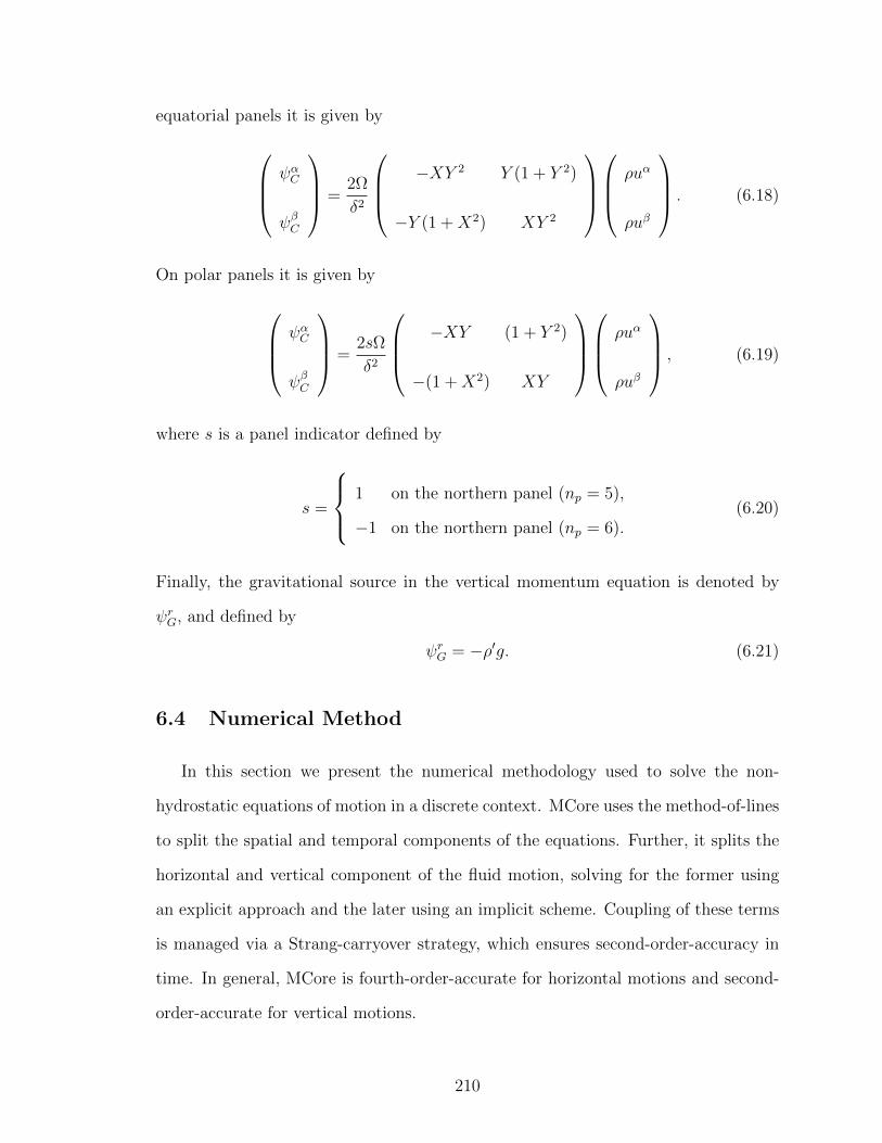
equatorial panels it is given by

ψαC

ψβC

=2Ω

δ2

−XY 2 Y (1 + Y 2)

−Y (1 +X2) XY 2

ρuα

ρuβ

. (6.18)

On polar panels it is given by

ψαC

ψβC

=2sΩ

δ2

−XY (1 + Y 2)

−(1 +X2) XY

ρuα

ρuβ

, (6.19)

where s is a panel indicator defined by

s =

1 on the northern panel (np = 5),

−1 on the northern panel (np = 6).(6.20)

Finally, the gravitational source in the vertical momentum equation is denoted by

ψrG, and defined by

ψrG = −ρ′g. (6.21)

6.4 Numerical Method

In this section we present the numerical methodology used to solve the non-

hydrostatic equations of motion in a discrete context. MCore uses the method-of-lines

to split the spatial and temporal components of the equations. Further, it splits the

horizontal and vertical component of the fluid motion, solving for the former using

an explicit approach and the later using an implicit scheme. Coupling of these terms

is managed via a Strang-carryover strategy, which ensures second-order-accuracy in

time. In general, MCore is fourth-order-accurate for horizontal motions and second-

order-accurate for vertical motions.

210

6.4.1 Finite-Volume Discretization

In this section we present the finite-volume discretization of the non-hydrostatic

equations using a high-order finite-volume scheme. Under the finite-volume approach,

we first integrate the Euler equations in the form (6.4)-(6.6) over an element Z (with

volume |Z|) and make use of Gauss’ divergence theorem to write the flux term as an

integral around the boundary ∂Z, giving

∂

∂tq +

1

|Z|

∫∫∂Z

F · ndS = ψM +ψC +ψG. (6.22)

Here the flux integral is taken over the surface with normal vector n and infinitesimal

area element dS. The term F · n is a vector quantity that denotes the outward flux

of each of the state variables perpendicular to the boundary. The double overline

denotes a 3D average of the form

φ =1

|Z|

∫Z

φdV. (6.23)

The term dV = Jdαdβdr denotes the infinitesimal volume element, which can vary

depending on the geometry. Here q denotes the averaged state vector in cell Z. Like-

wise, ψM denotes the element-averaged source terms due to the underlying geometry,

whereas ψC and ψG respectively denote the source terms due to the Coriolis force

and gravity. Note that the volume-averaged formulation (6.22) is exactly equivalent

to the original non-hydrostatic equations, and it is left to us to define an appropriate

discretization over each of the terms in this expression.

In order to simplify the discussion on the computational implementation, we dis-

tinguish between the computational domain and physical domain. The physical do-

main on each panel consists of the region bounded by (α, β) ∈ [−π/4, π/4]2 in the

horizontal and the region between the planetary surface, defined by rs(α, β, np), and

211

the fixed-height rigid-lid rT in the vertical. On the other hand, the computational do-

main is the continuous analog of the physical domain in computer memory. On each

panel it consists of a horizontal region bounded by (α, β) ∈ [−π/4, π/4]2, but in the

vertical uses an auxiliary coordinate ξ ∈ [0, 1]. Importantly, grid elements must be

uniform in computational space along each coordinate direction; that is, grid elements

all have horizontal extent ∆α (in α and β) and vertical extent ∆ξ = 1/Nr (where Nr

is the discrete vertical integer resolution). This implies that surfaces of constant ξ are

also the vertical bounding surfaces of model levels. An invertible conformal mapping

is defined that takes a point in the computational domain to the physical domain via

Φ : (ξ, α, β, np)→ (R(ξ;α, β, np), α, β, np). (6.24)

Note that R(ξ) : [0, 1] → [rs(α, β, np), rT ] must be bijective and monotonically in-

creasing in ξ. In real atmospheric simulations, the function R can be chosen to place

additional grid resolution near the surface. In section 6.5 we give one possible choice

of R, which will be used in our simulations.

For all arrays which are defined over the grid, there must exist a uniform mapping

between array indices and computational space. Element centroids, for instance, are

denoted by integer sub-indices, and over a single cubed-sphere panel are given by

αi =

(i+

1

2

)∆α− π

4, βj =

(j +

1

2

)∆α− π

4, ξk =

(k +

1

2

)∆ξ. (6.25)

The indices span the range (i, j) ∈ [1, Nc]2 and k ∈ [1, Nr]. The radial coordinate of

element centroids is defined by mapping ξk to physical space,

rk = R(ξk;αi, βi, np). (6.26)

Note that k = 1 corresponds to the lowermost model level whereas k = Nr corresponds

212

to the uppermost model level, which is the opposite of most pressure-based hydrostatic

model formulations.

Faces are midway between neighboring element centroids, and so are defined by

half-indices and denoted by the symbol ∂Z. For example, the edge ∂Zi+1/2,j,k is at the

interface between element (i, j, k) and (i+ 1, j, k) and defines a plane that is constant

in both α and β. Radial faces, denoted by ∂Zi,j,k+1/2 are constant in ξ, but are not

necessarily constant in r due to the horizontal dependence of the mapping R. In fact,

they are defined by the two-dimensional surface r −R(ξ;α, β, np) = 0 for ξ fixed.

In the finite-volume discretization we must make use of both element volumes,

denoted by |Z|, and face areas, denoted by |∂Z|. In terms of the metric Jacobian

(H.1), the element volume takes the form

|Z|i,j,k =

∫Z

dV =

αi+1/2∫αi−1/2

βj+1/2∫βj−1/2

rk+1/2∫rk−1/2

Jdrdβdα. (6.27)

The area of faces is likewise calculated by integrating the infinitesimal face areas

(G.6)-(G.8). In practice these integrals are pre-computed using high-order Gaussian

quadrature and stored for later use.

Quantities which are defined as edge averages will be denoted by a single overline.

Average fluxes are defined at element faces and denoted here by Fi+1/2,j,k for a flux

across face (i+ 1/2, j, k). They are defined by

Fi+1/2,j,k =1

|∂Z|i+1/2,j,k

∫∫∂Zi+1/2,j,k

F · ndS, (6.28)

where |∂Z|i+1/2,j,k denotes the area of the face. Hence, the total flux across an inter-

face, here denoted by Fi+1/2,j,k, is simply the product of the average flux and the face

area

Fi+1/2,j,k = Fi+1/2,j,k |∂Z|i+1/2,j,k. (6.29)

213

Using (6.29) the volume averaged formulation (6.22) can be rewritten as

∂

∂tqi,j,k = H(q) + V(q), (6.30)

where

H(q) =1

|Z|i,j,k[Fi−1/2,j,k − Fi+1/2,j,k + Fi,j−1/2,k − Fi,j+1/2,k

]+ ψM + ψC ,(6.31)

and

V(q) =1

|Z|i,j,k[Fi,j,k−1/2 − Fi,j,k+1/2

]+ ψG. (6.32)

Here we utilize a splitting based on separating horizontal motions, denoted by H(q),

and vertical motions, denoted by V(q). Numerically this splitting is desirable since

the relatively small vertical spacing of elements (on the scale of tens to hundreds of

meters) imposes a severe timestep restriction via the CFL condition. Hence, if we

make use of an explicit treatment of the horizontal motions and treat the vertical

motions implicitly, the model timestep will not be affected by the grid spacing in the

vertical.

6.4.2 Horizontal Reconstruction

Under the finite-volume formulation only element-averaged information is known

within each element. Hence, a sub-grid-scale reconstruction can only be built using

information from neighboring elements. MCore uses a novel reconstruction strategy

which attains fourth-order accuracy using a minimal set of neighboring elements.

In general, attaining greater than second-order accuracy is difficult since a O(∆αn)

reconstruction requires that the pth derivatives be approximated to O(∆αn−p). Stan-

dard finite-difference reconstruction formulae only guarantee O(∆α2) accuracy, since

such an approach approximates cell-centerpoint values using cell-averaged values. In

214

a non-Cartesian domain, reconstructions must also incorporate information about

the underlying geometry to recover high-order accuracy. For simplicity, we choose to

drop the vertical index k in this section since the horizontal reconstruction process is

applied on each vertical level separately.

The strategy we have introduced relies on the convolution and deconvolution pro-

cedure of Barad and Colella (2005). This approach provides a mechanism for trans-

forming cell-averages to cell-centered point values over a sufficiently smooth data field,

according to

φ(0) = φ− ∆α4

12|Z|

(∂φ

∂α

∂J

∂α+∂φ

∂β

∂J

∂β

)− ∆α2

24

(∂2φ

∂α2+∂2φ

∂β2

), (6.33)

where J is the radially-integrated Jacobian,

J(α, β, np) =

R(ξk+1/2;α,β,np)∫R(ξk−1/2;α,β,np)

J(r, α, β, np)dr. (6.34)

If φi,j is known to at least fourth-order accuracy and the remaining derivative terms

are known to at least O(∆α2), this formula leads to a fourth-order-accurate approxi-

mation of φ(0)i,j, the cell-centered value of φ in element (i, j). In this formulation, we

directly approximate the derivatives of the radially-integrated Jacobian by

∂J

∂α≈ |Z|i+1,j − |Z|i−1,j

2∆α, (6.35)

∂J

∂β≈ |Z|i,j+1 − |Z|i,j−1

2∆α. (6.36)

For reasons of efficiency, these derivative are pre-computed prior to the simulation

and stored for later use.

The reconstruction used by MCore proceeds as follows. The stencil we will use in

the reconstruction step is depicted in Figure 6.2. Second and third derivatives are first

215

Figure 6.2:A depiction of the stencil used for computing the fourth-order sub-grid-scale reconstruction on the cubed-sphere.

calculated using standard finite-difference formulae, which leads to approximations

which are O(∆α2) accurate. Here we use q to denote one element of the state vector

q.

Dαααqi,j =qi+2,j − 2qi+1,j + 2qi−1,j − qi−2,j

12∆α3, (6.37)

Dααβqi,j =qi+1,j+1 − qi+1,j−1 − 2qi,j+1 + 2qi,j−1 + qi−1,j+1 − qi−1,j−1

4∆α3, (6.38)

Dαββqi,j =qi+1,j+1 − 2qi+1,j + qi+1,j−1 − qi−1,j+1 + 2qi−1,j − qi−1,j−1

4∆α3, (6.39)

Dβββqi,j =qi,j+2 − 2qi,j+1 + 2qi,j−1 − qi,j−2

12∆α3. (6.40)

216

Dααqi,j =−qi+2,j + 16qi+1,j − 30qi,j + 16qi−1,j − qi−2,j

24∆α2, (6.41)

Dαβqi,j =qi+1,j+1 − qi−1,j+1 − qi+1,j−1 + qi−1,j−1

4∆α2, (6.42)

Dββqi,j =−qi,j+2 + 16qi,j+1 − 30qi,j + 16qi,j−1 − qi,j−2

24∆α2. (6.43)

To attain fourth-order accuracy in space, we require that our approximation to

the first derivative terms be at least O(∆α3). To construct such a formula, we utilize

a finite-difference relation over element point-values which have been reconstructed

to O(∆α4). First, define O(∆α2) approximations to the first derivatives by

D∗αqi,j =−qi+2,j + 8qi+1,j − 8qi−1,j + qi−2,j

12∆α, (6.44)

D∗βqi,j =−qi,j+2 + 8qi,j+1 − 8qi,j−1 + qi,j−2

12∆α. (6.45)

High-order element averages of the state vector which do not incorporate geometric

terms can then be computed via

q∗i+m,j = qi+m,j −∆α4

12|Z|i+m,j

(D∗αqi,j +m∆αDααqi,j)

(∂J

∂α

)i+m,j

(6.46)

+(D∗βqi,j +m∆αDαβqi,j

)(∂J∂β

)i+m,j

,and

q∗i,j+m = qi,j+m −∆α4

12|Z|i,j+m

(D∗αqi,j +m∆αDαβqi,j)

(∂J

∂α

)i,j+m

(6.47)

+(D∗βqi,j +m∆αDββqi,j

)(∂J∂β

)i,j+m

.

217

A third-order approximation to the first derivative terms is then given by

Dαqi,j =−q∗i+2,j + 8q∗i+1,j − 8q∗i−1,j + q∗i−2,j

12∆α− ∆α2

24(Dαααqi,j +Dαββqi,j) ,(6.48)

Dβqi,j =−q∗i,j+2 + 8q∗i,j+1 − 8q∗i,j−1 + q∗i,j−2

12∆α− ∆α2

24(Dααβqi,j +Dβββqi,j) (6.49)

A fourth-order approximation to the element centerpoint value is similarly obtained

from the relation

q(0)i,j = qi,j−∆α2

12|Z|i,j

Dαqi,j

(∂J

∂α

)i,j

+Dβqi,j

(∂J

∂β

)i,j

−∆α2

24[Dααqi,j +Dββqi,j] .

(6.50)

We make no attempt at introducing a limiter for enforcing monotonicity or pos-

itivity of thermodynamic quantities. Limiting is generally of greater importance for

tracer transport problems where monotonicity and positivity must be guaranteed,

and so it is not pursued here.

With the approximated centerpoint value and corresponding derivatives in hand,

we can now write expressions for the reconstructed state vector at face centerpoints.

These face centerpoint values are denoted with either a L or R, denoting whether

they are left or right of the interface:

qL,i+1/2,j = q(0)i,j +Dαqi,j

(∆α

2

)+Dααqi,j

(∆α

2

)2

+Dαααqi,j

(∆α

2

)3

,(6.51)

qR,i−1/2,j = q(0)i,j −Dαqi,j

(∆α

2

)+Dααqi,j

(∆α

2

)2

−Dαααqi,j

(∆α

2

)3

,(6.52)

qL,i,j+1/2 = q(0)i,j +Dβqi,j

(∆α

2

)+Dββqi,j

(∆α

2

)2

+Dβββqi,j

(∆α

2

)3

,(6.53)

qR,i,j−1/2 = q(0)i,j −Dβqi,j

(∆α

2

)+Dββqi,j

(∆α

2

)2

−Dβββqi,j

(∆α

2

)3

.(6.54)

The centerpoint values, as calculated from the above formulae are then used for

computing edge fluxes across the interface via a Riemann solver. This calculation

218

will be described in more detail later.

6.4.3 Vertical Reconstruction

In the vertical we can no longer rely on uniformity of the grid spacing, so the recon-

struction must take into account the variance in the height of grid elements. Nonethe-

less, we can still construct a second-order sub-grid-scale reconstruction within each

element by fitting a parabola through the centroid of each grid element and its imme-

diate neighbors. As a result, we obtain the following formulae for the reconstructed

field at each edge:

qL,k+1/2 = −∆r2

p

4∆rn(∆rn + ∆rp)qk−1 +

(2∆rn + ∆rp)

4∆rnqk +

(2∆rn + ∆rp)

4(∆rn + ∆rp)qk+1,(6.55)

qR,k−1/2 =(∆rn + 2∆rp)

4(∆rn + ∆rp)qk−1 +

(∆rn + 2∆rp)

4∆rpqk −

∆r2n

4∆rp(∆rp + ∆rn)qk+1,(6.56)

where

∆rp = rk+1 − rk, ∆rn = rk − rk−1. (6.57)

Unlike in the horizontal, the subscripts L and R actually correspond to the elements

immediately below and immediately above each edge, respectively.

Near the top and bottom boundaries, the stencil width is reduced by one element

and so the sub-grid-scale reconstruction becomes linear. At the bottom boundary the

reconstruction then reads

qR,1/2 =(2∆rn + ∆rp)

∆rn + ∆rpq1 −

∆rn∆rn + ∆rp

q2, (6.58)

qL,3/2 =∆rp

∆rp + ∆rnq1 +

∆rn∆rp + ∆rn

q2, (6.59)

where

∆rp = r3 − r2, ∆rn = r2 − r1. (6.60)

219

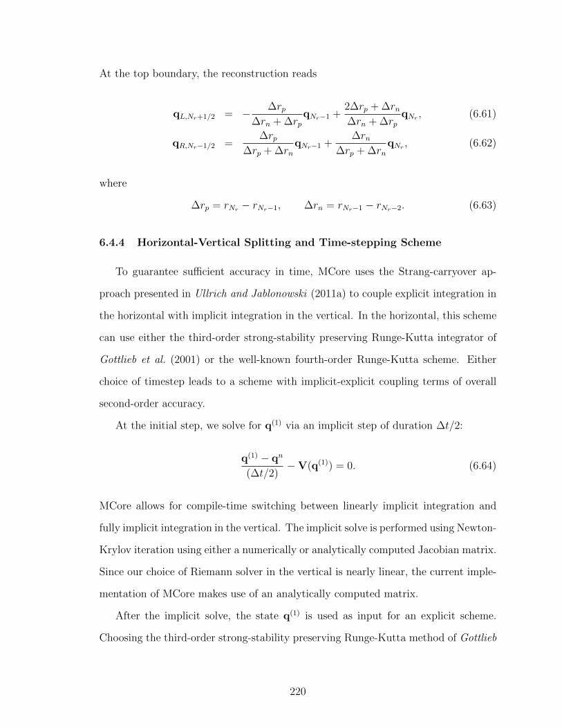
At the top boundary, the reconstruction reads

qL,Nr+1/2 = − ∆rp∆rn + ∆rp

qNr−1 +2∆rp + ∆rn∆rn + ∆rp

qNr , (6.61)

qR,Nr−1/2 =∆rp

∆rp + ∆rnqNr−1 +

∆rn∆rp + ∆rn

qNr , (6.62)

where

∆rp = rNr − rNr−1, ∆rn = rNr−1 − rNr−2. (6.63)

6.4.4 Horizontal-Vertical Splitting and Time-stepping Scheme

To guarantee sufficient accuracy in time, MCore uses the Strang-carryover ap-

proach presented in Ullrich and Jablonowski (2011a) to couple explicit integration in

the horizontal with implicit integration in the vertical. In the horizontal, this scheme

can use either the third-order strong-stability preserving Runge-Kutta integrator of

Gottlieb et al. (2001) or the well-known fourth-order Runge-Kutta scheme. Either

choice of timestep leads to a scheme with implicit-explicit coupling terms of overall

second-order accuracy.

At the initial step, we solve for q(1) via an implicit step of duration ∆t/2:

q(1) − qn

(∆t/2)−V(q(1)) = 0. (6.64)

MCore allows for compile-time switching between linearly implicit integration and

fully implicit integration in the vertical. The implicit solve is performed using Newton-

Krylov iteration using either a numerically or analytically computed Jacobian matrix.

Since our choice of Riemann solver in the vertical is nearly linear, the current imple-

mentation of MCore makes use of an analytically computed matrix.

After the implicit solve, the state q(1) is used as input for an explicit scheme.

Choosing the third-order strong-stability preserving Runge-Kutta method of Gottlieb

220

et al. (2001) leads to

q(2) = q(1) + ∆tH(q(1)), (6.65)

q(3) =3

4q(1) +

1

4q(2) +

∆t

4H(q(2)), (6.66)

q∗ =1

3q(1) +

2

3q(3) +

2∆t

3H(q(3)). (6.67)

The fourth-order Runge-Kutta scheme instead leads to the sequence

q(2) = q(1) +∆t

2H(q(1)), (6.68)

q(3) = q(1) +∆t

2H(q(2)), (6.69)

q(4) = q(1) + ∆tH(q(3)), (6.70)

q∗ = −1

3q(1) +

1

3q(2) +

2

3q(3) +

1

3q(4) +

∆t

6H(q(4)). (6.71)

Finally, q∗ becomes the input for a final implicit solve of size ∆t/2:

qn+1 − q∗

(∆t/2)−V(qn+1) = 0. (6.72)

The forcing due to the implicit step is then stored

G = qn+1 − q∗. (6.73)

At the following timestep, the implicit forcing from the previous timestep is used to

predict the next input for the explicit scheme,

q(1) = qn + G. (6.74)

Observe that after the initial step, the resulting scheme only uses one implicit solve

per timestep.

221

6.4.5 Orthonormalization

MCore makes use of approximate Riemann solvers for computing the flux F(q)

across each face. However, generic Riemann solvers are purely one-dimensional op-

erators. To apply this class of solvers to multidimensional problems, we must first

transform vector quantities into an orthonormal frame. In 3D, the orthonormal frame

consists of one basis vector which is orthogonal to the active edge (denoted e⊥) and

two components which are parallel to the edge (denoted e1 and e2). Hence, the

non-orthogonal components define a tangent plane to the active edge. At the point

where the orthogonal basis is defined, an arbitrary vector can be written in either the

natural basis,

v = vαgα + vβgβ + vrgr, (6.75)

or in the orthonormal basis

v = v⊥e⊥ + v1e1 + v2e2. (6.76)

The transformation between these two systems is accomplished via the orthonormal-

ization matrix Od(α, β, r),

v⊥

v1

v2

= Od(α, β, r)

vα

vβ

vr

. (6.77)

Here d denotes the coordinate being held constant, d ∈ α, β, ξ. Analogously, trans-

forming from the orthonormal basis to the natural basis simply requires applying the

inverse operation, vα

vβ

vr

= O−1d (α, β, r)

v⊥

v1

v2

. (6.78)

222

Since the natural basis for the cubed-sphere consists of a radial basis vector which

is already normalized and orthogonal to the basis vectors in the horizontal, at edges

of constant α and constant β, we simply set e2 = gr. The orthonormalization matrix

at edges of constant α can then be written as a 2× 2 matrix,

Oα =

√

1 +X2

δ0

−XY√

1 +X2

δ2

(1 + Y 2)√

1 +X2

δ2

. (6.79)

Similarly, at edges of constant β we have

Oβ =

0

√1 + Y 2

δ

(1 +X2)√

1 + Y 2

δ2

−XY√

1 + Y 2

δ2

. (6.80)

In each case the matrices defined above only work on the horizontal components of

the vector v. The corresponding deorthonormalization matrices are

O−1α =

δ√

1 +X20

XY δ

(1 + Y 2)√

1 +X2

δ2

(1 + Y 2)√

1 +X2

, (6.81)

O−1β =

XY δ

(1 +X2)√

1 + Y 2

δ2

(1 +X2)√

1 + Y 2

δ√1 + Y 2

0

. (6.82)

The problem of deriving an orthonormalization matrix in the vertical is more

difficult since a cell’s vertical bounding surface (a surface of constant ξ) is only a

surface of constant r in the absence of terrain. When terrain is present, we utilize

the fact that ∇if defines a vector perpendicular to the surface f(α, β, r) = r −

223

R(ξ;α, β, np) (with ξ = const.). Hence, the vector

e∗⊥ =

[[G11

(−∂R∂α

)+G12

(−∂R∂β

)]gα +

[G21

(−∂R∂α

)+G22

(−∂R∂β

)]gβ + gr

],

(6.83)

is orthogonal to the given terrain-following radial face (but is not of unit length). A

vector of unit length can be obtained by simply scaling e∗⊥ according to

e⊥ =1

|e∗⊥|e∗⊥, (6.84)

where |v| =√Gijvivj is the magnitude of the vector in cubed-sphere coordinates.

Hereafter we use eα⊥, eβ⊥ and er⊥ to denote the components of e⊥ along the α, β and r

directions. To obtain vectors orthogonal to e⊥, we simply apply the Gram-Schmidt

orthonormalization procedure to the α and β components of the natural basis. For

example, for the α component, we have

e∗1 = gα − 〈gα, e⊥〉e⊥, (6.85)

with curvilinear inner product 〈v,w〉 = Gijviwj. Hence, on simplifying,

e∗1 = (1−Qαeα⊥)gα −Qαeβ⊥gβ −Qαer⊥gr, (6.86)

where Qα = G11eα⊥ +G12e

β⊥. Similarly,

e∗2 = −Qβeα⊥gα + (1−Qβeβ⊥)gβ −Qβer⊥gr, (6.87)

where Qβ = G21eα⊥+G22e

β⊥. As before, we normalize these vectors to obtain e1 and e2.

The deorthonormalization matrix O−1ξ is then defined as the matrix whose columns

are given by e⊥, e1 and e2. To obtain Oξ at each edge, we invert the corresponding

deorthonormalization matrix numerically.

224

In the formulation used by MCore, the orthonormalization and deorthonormaliza-

tion matrices are only required at the centerpoint of each face. Hence, these matrices

can be pre-computed, for reasons of efficiency, and stored for later use. After certain

optimizations to the algorithmic implementation of the Riemann solver, it turns out

that only three components of each of the matrices are required during runtime.

6.4.6 Riemann Solvers

Under any upwind finite-volume formulation, reconstructed edge values are in-

herently discontinuous – that is, the reconstructed left edge value is almost never

identically equal to the right edge value. The discrepancy between left and right edge

values is a measure of the roughness of the underlying fields. Godunov-type finite-

volume methods (Godunov , 1959), such as the one in this chapter, solve the Riemann

problem at interfaces so as to obtain a single-valued flux at each edge. Since com-

puting the exact solution of the Riemann problem is generally expensive, we instead

rely on so-called approximate Riemann solvers. However, dozens of such approximate

solvers are now available. Ullrich et al. (2010) analyzed three such solvers, including

the solver of Rusanov (1961), the solve of Roe (1981) and the recently introduced

AUSM+-up solver of Liou (2006). They concluded that for horizontal atmospheric

motions the Rusanov solver was far too diffusive, whereas both Roe and AUSM+-up

yielded comparable results, with AUSM+-up slightly outperforming Roe.

Based on the results of Ullrich et al. (2010) we have adopted the AUSM+-up solver

for computing fluxes. The details of this Riemann solver are given in Liou (2006), and

so the algorithm is not repeated here. The only notable change in our implementation

is the choice of Ku = 0, instead of Liou’s suggested choice Ku = 1/4. In the vertical

we make use of a linearized variant of the AUSM+-up flux, as this method has been

shown to be very effective in the extremely low Mach number regime.

The AUSM+-up Riemann solver was originally designed with the low-Mach num-

225

ber limit in mind. Many Riemann solvers introduce diffusion that is proportional

to the sound speed over all state variables, which is potentially disastrous for accu-

rate modeling of flows in the low-Mach number limit. For general low-Mach number

flows, Liou showed that a better characterizations of numerical diffusion can be ob-

tained by asymptotic analysis. For very low-speed flows, such as vertical atmospheric

motions, Liou’s solver can be simplified further by linearizing the diffusive terms.

This approach was used in Ullrich and Jablonowski (2011a) to define a quasi-linear

AUSM+-up variant for vertical motions. This strategy is desirable since the resulting

Jacobian takes on a simple analytic form that can be efficiently implemented in an

implicit solver.

The quasi-linear AUSM+-up solver makes use of the hydrostatic background state

to define a background sound speed ch1/2 =√γph/ρh at each vertical interface (with

γ = cp/cv). Given left and right state vectors qL = (ρL, (ρu)L, (ρθ)L) and qR =

(ρR, (ρu)R, (ρθ)R), we define a modified velocity at the interface via

w1/2 =(ρv⊥)L + (ρv⊥)R

ρL + ρR−Kpc

h1/2

(ρθ)R − (ρθ)L(ρθ)h

, (6.88)

where Kp is the dimensionless pressure diffusion coefficient and (ρθ)h is the potential

temperature density of the hydrostatic background at the interface. Similarly, we

define an interface pressure using (6.7) that is given by

p1/2 = p0

(Rd

p0

((ρθ)L + (ρθ)R

2

))cp/cv− Ku

2c1/2((ρv⊥)R − (ρv⊥)L), (6.89)

where ph is the hydrostatic pressure at the interface and Ku is the dimensionless

momentum diffusion coefficient. The pointwise flux across the interface is then defined

by

FAUSM(0) = p′1/2 +

w1/2qL if w1/2 > 0,

w1/2qR otherwise,(6.90)

226

where

p′1/2 =(0, p1/2 − ph1/2, 0, 0, 0

), (6.91)

i.e. p1/2 only has one non-zero value, which is a contribution associated with the

perpendicular component of the momentum. This solver uses tuning parameters Ku

and Kp, which have been chosen as Ku = 2 and Kp = 1/4. In Ullrich and Jablonowski

(2011a) we have observed that this larger value of Ku is required to damp spurious

vertical oscillations when the aspect ratio is large (as opposed to the recommended

value of 3/4 given in Liou (2006)). Finally, since the vertical flux is only second-order

accurate, we make the approximation

Fi,j,k+1/2 = F(0)i,j,k+1/2, (6.92)

i.e. we take the average flux across the interface to be equal to the pointwise flux

evaluated from (6.90).

6.4.7 Fourth-order Horizontal Accuracy

To solve for the flux across horizontal faces we make use of the reconstructed values

of the state variables on either side of the interface. Fluxes are evaluated pointwise

at element face centerpoints, and are obtained by solving a Riemann problem using

left and right state vectors. The resulting pointwise flux vector is a second-order

approximation to the average flux across the interface. To obtain fourth-order accu-

racy in computing the flux across the interface, some form of high-order quadrature is

needed. In this section we again drop the vertical index k, which is assumed constant.

MCore makes use of a convolution formula for computing average face fluxes F

227

from pointwise fluxes F(0). On faces of constant α and β, this formula takes the form

Fi+1/2,j = F(0)i+1/2,j +∆α2

24

(∂2F

∂β2

)i+1/2,j

+∆α2

12|∂Z|i+1/2,j

(∂F

∂β

)i+1/2,j

(∂Jα∂β

)i+1/2,j

,(6.93)

Fi,j+1/2 = F(0)i,j+1/2 +∆α2

24

(∂2F

∂α2

)i,j+1/2

+∆α2

12|∂Z|i,j+1/2

(∂F

∂α

)i,j+1/2

(∂Jβ∂α

)i,j+1/2

.(6.94)

Here Jα and Jβ are the radially-integrated metric co-factors (H.2)-(H.3). Under our

formulation, their derivatives are approximated in terms of neighboring face areas as

(∂Jα∂β

)i+1/2,j

≈|∂Z|i+1/2,j+1 − |∂Z|i+1/2,j−1

2∆α, (6.95)

and (∂Jβ∂α

)i+1/2,j

≈|∂Z|i+1,j+1/2 − |∂Z|i−1,j+1/2

2∆α. (6.96)

To maintain fourth-order-accuracy, the pointwise fluxes in (6.93) and (6.94) must

be evaluated to at least O(∆α4) and flux derivative terms must be evaluated at

O(∆α2). Hence, it is sufficient to make use of the compact second-order derivative

formulae

(∂F

∂β

)i+1/2,j

≈F(0)i+1/2,j+1 − F(0)i+1/2,j−1

2∆α, (6.97)(

∂2F

∂β2

)i+1/2,j

≈F(0)i+1/2,j+1 − 2F(0)i+1/2,j + F(0)i+1/2,j−1

∆α2, (6.98)(

∂F

∂α

)i,j+1/2

≈F(0)i+1,j+1/2 − F(0)i−1,j+1/2

2∆α, (6.99)(

∂2F

∂α2

)i,j+1/2

≈F(0)i+1,j+1/2 − 2F(0)i,j+1/2 + F(0)i−1,j+1/2

∆α2. (6.100)

To achieve fourth-order accuracy overall, source terms of the horizontal momen-

tum equations must be evaluated to at least third-order accuracy. As with edge

fluxes, simply evaluating the source terms using cell-averaged values qi,j,k only leads

228

to a second-order discretization. Hence, MCore follows a convolution and deconvolu-

tion strategy that leads to a fourth-order-accurate approximation of the source terms.

To begin, source terms are first evaluated at element centerpoints (ψ(0)i,j = ψ(q(0)i,j)).

Notably, the state vector q(0)i,j has already been calculated at this point during re-

construction using (6.50). Now, to obtain a fourth-order accurate approximation to

the forcing term within this element we apply a convolution operator of the form

ψi,j = ψ(0)i,j +∆α2

24

[(∂2ψ

∂α2

)i,j

+

(∂2ψ

∂β2

)i,j

]+

∆α4

12|Z|i,j

[∂ψ

∂α

∂J

∂α+∂ψ

∂β

∂J

∂β

]. (6.101)

As with the flux operators, all first and second derivatives are approximated to second-

order accuracy using standard centered finite-difference operators. The derivatives of

the vertically-integrated metric Jacobian are approximated by (6.35)-(6.36).

6.4.8 Inclusion of Topography

Topography does not explicitly enter the formulation of MCore, but instead en-

ters implicitly in two ways. First, element volumes and face areas are modified by

the presence of topography. This has a direct effect on the calculation of total edge

fluxes. Notably, under the shallow-atmosphere approximation the areas of vertical

bounding faces are actually unmodified by the presence of topography. The second

method topography enters the formulation is via pressure terms that are accounted

for by the deorthonormalization matrix. Namely, when fluxes are computed across

vertical surfaces the deorthonormalization procedure is responsible for applying pres-

sure forcing appropriately to all components of the momentum. This has the effect

of applying pressure forcing to the horizontal momentum components whenever the

vertical bounding face is tilted, such as in the presence of topography.

229

6.4.9 Treatment of Panel Boundaries

One must be careful in the treatment of panel boundaries on the cubed-sphere

grid. First, the underlying coordinate system is disjoint at panel boundaries so one

must be certain that vector quantities are in the correct reference frame. Second, since

the grid is not smooth in the vicinity of the panel boundary a direct application of the

reconstruction stencil near grid edges can potentially generate significant numerical

noise and reduce the accuracy of the simulation. As a consequence, we advocate the

use of halo elements around panels (see Figure 6.1) in combination with an appropriate

remapping algorithm.

The remapping process we apply in MCore is identical to the one described in

Ullrich et al. (2010). Under this approach, halo elements are extended outward from

each panel. Sub-grid-scale fourth-order reconstructions are built along each panel

edge using one-sided reconstruction stencils and the reconstructions are sampled at

Gaussian quadrature points. As a result, we obtain fourth-order-accurate approxi-

mations to element averages in halo elements. The usual horizontal reconstruction

stencil can then be applied, minimizing the generation of spurious boundary noise.

6.4.10 Rayleigh Friction

It is well-known that atmospheric models that have a rigid-lid upper boundary

condition typically suffer significant wave reflection at the model top. The traditional

approach to deal with this problem has been to add a sponge layer that is responsible

for damping out oscillations in the velocity fields high in the atmosphere. Wave

reflection is particularly problematic near steep topography or in the presence of

strong vertical motions.

MCore implements an optional Rayleigh friction layer. Since Rayleigh friction is

a potentially stiff effect, it is included in the implicit stage of the solver as a source

230

term of the full 3D momentum equation that takes the form

ψR = −Rc(α, β, ξ)(ρu− ρu0), (6.102)

where Rc denotes the strength of the friction term, u is the 3D velocity vector and u0

denotes some appropriate reference state for the velocity. The strength of the friction

term can be chosen arbitrarily, but should transition smoothly from zero forcing at

lower levels to some maximum at the model top. For simplicity, we choose

Rc(α, β, ξ) =

0 if ξ < ξR,

1

τR

(ξ − ξR1− ξR

)2

otherwise.

(6.103)

Here τR is the timescale of the damping and ξR is the height of the damping layer in

ξ coordinates. By default, we define τR = 1 day and ξR = 0.7, which roughly places

the Rayleigh damping layer at an altitude of 20 km.

6.4.11 Design Features

The high-order finite-volume methods of MCore are designed to allow run-time

switching between shallow-water, shallow-atmosphere and deep-atmosphere approxi-

mations. Further, compile-time switching is available for the choice of time-discretization,

the form of the non-hydrostatic evolution equations, the choice of Riemann solver and

the form of the horizontal reconstruction. The model attempts to maximize efficiency

by pre-computing geometric quantities and storing the corresponding values for the

duration of the simulation. To enhance modularity and readability the model is

implemented in C++ using classes to isolate functionality.

MCore makes use of the GECoRe remapping package of Ullrich et al. (2009)

for performing conservative remapping between cubed-sphere and latitude-longitude

grids. The data output format can be chosen to be MATLAB-readable .mat files or

231

NetCDF .nc data.

6.5 Numerical Results

Several test cases have been chosen to demonstrate the robustness and accuracy

of MCore, including a baroclinic instabilty, mountain-induced Rossby wave train and

a 3D Rossby-Haurwitz wave. Rayleigh friction, as described in section 6.4.10, is only

used for the mountain-induced Rossby wave train test case. All test runs make use

of a rT = 30 km model top and a vertical grid spacing which we have chosen to be

R(ξ;α, β, np) = rs(α, β, np) + (rT − rs(α, β, np))φ(ξ), (6.104)

where

φ(ξ) =1√

b+ 1− 1

[√bξ2 + 1− 1

]. (6.105)

Recall that ξ specifies the auxiliary vertical coordinate, which is defined on the in-

terval [0, 1] at each point (α, β, np). This choice of vertical grid spacing is chosen to

match operational conditions, where additional resolution is generally desired near

the surface. Here b is a flattening parameter which we choose to be b = 10. It

determines how quickly model levels tend towards equal spacing at higher altitudes.

All model runs have taken place on a c90 grid with 26 vertical levels. Namely, on

each model level the grid consists of the six panels of the cubed-sphere each being

subdivided into a 90 × 90 grid of elements. This choice corresponds to a RLL grid

with one degree grid spacing at the equator, although overall the cubed-sphere grid

has 25% fewer elements than such a RLL grid. We make use of the RK4 timestepping

strategy (6.68)-(6.71) for the explicit integration with a fixed timestep of ∆t = 200 s.

All of the test cases examined in this document are written in terms of spherical

coordinates with longitude λ and latitude ϕ. Coordinate transforms are provided in

Appendix G for translating these quantities to the cubed-sphere.

232

6.5.1 Baroclinic Instability

The baroclinic instability test of Jablonowski and Williamson (2006) has become

an important test case for hydrostatic dynamical cores. Although this test is ideal-

ized, the background field is chosen to closely resemble the known background state

of the true atmosphere. As such, this test may shed light into the treatment of real

atmospheric motions by the atmospheric model. This test case was originally formu-

lated in so-called η pressure coordinates, which are defined by η = p/ps, and so had

to be remapped to height coordinates before being used in MCore.

This test utilizes an auxiliary variable ην , defined by

ην = (η − η0)π

2, (6.106)

with η0 = 0.252. The flow field for this test consists of two symmetric zonal jets in

the midlatitudes, utilizing a wind field defined in spherical coordinates via

u(λ, ϕ) = u0 cos32 ην sin2(2ϕ), (6.107)

v(λ, ϕ) = 0, (6.108)

w(λ, ϕ) = 0. (6.109)

Here the maximum amplitude u0 is set to 35 m s−1. The horizontally averaged

temperature T (η) is split into representations of the lower and middle atmosphere,

T (η) = T0ηRdΓ

g (for η ≥ ηt), (6.110)

T (η) = T0ηRdΓ

g + ∆T (ηt − η)5 (for ηtop > η) (6.111)

with the tropopause level chosen to be ηt = 0.2, horizontal mean temperature of

the surface T0 = 288 K, lapse rate Γ = 0.005 K m−1 and empirical temperature

233

difference ∆T = 4.8 × 105 K. The total temperature distribution is the sum of the

mean temperature distribution and a horizontal variation at each level,

T (λ, ϕ, η) = T (η) +3

4

ηπu0

Rd

sin ην cos12 ην ×(

−2 sin6 ϕ

(cos2 ϕ+

1

3

)+

10

63

)2u0 cos

32 ην+(

8

5cos3 ϕ

(sin2 ϕ+

2

3

)− π

4

)aΩ

. (6.112)

The geopotential Φ = gz completes the definition of the steady-state conditions. As

with the temperature field, we define a horizontally averaged geopotential

Φ(η) =T0g

Γ

(1− η

RdΓ

g

)(for η ≥ ηt)

(6.113)

Φ(η) =T0g

Γ

(1− η

RdΓ

g

)−Rd∆T× (for ηtop > η)

(6.114)(ln

(η

ηt

)+

137

60

)η5t − 5η4

t η + 5η3t η

2 − 10

3η2t η

3 +5

4ηtη

4 − 1

5η5

.

The total geopotential is then determined by

Φ(λ, ϕ, η) = Φ(η) + u0 cos32 ην ×(

−2 sin6 ϕ

(cos2 ϕ+

1

3

)+

10

63

)u0 cos

32 ην+(

8

5cos3 ϕ

(sin2 ϕ+

2

3

)− π

4

)aΩ

. (6.115)

The above formulation describes a state which is in both hydrostatic and geostrophic

balance, and hence in a perfect model it should be maintained indefinitely. However,

numerical errors due to the discretization will nonetheless creep into the solution and

cause the steady nature of this profile to be lost. These errors eventually accumulate

234

and result in the collapse of the flow into turbulent motions which are determined by

the discrete properties of the numerical method.

In order to trigger an instability which is more deterministic in its evolution,

Jablonowski and Williamson (2006) introduce an overlaid perturbation in the zonal

velocity field. They select a Gaussian profile centered at (λc, ϕc) = (π/9, 2π/9), which

leads to an instability in the northern jet. The perturbation is Gaussian, given by

u′(λ, ϕ, η) = up exp

(−(rcR

)2), (6.116)

with radius R = a/10 and maximum amplitude up = 1m s−1. Here rc is the great

circle distance

rc = a arccos [sinϕc sinϕ+ cosϕc cosϕ cos(λ− λc)] . (6.117)

The hydrostatic background state for these simulations is given by the initial

conditions. In figure 6.3 we plot snapshots of the baroclinic wave test case at day 7 and

9 showing surface pressure, 850 hPa temperature and 850 hPa relative vorticity. All

results are interpolated to pressure levels from heigh levels using a linear interpolant.

An intercomparison of the performance of various dynamical cores on this test case

can be found in Lauritzen et al. (2010). The results from MCore are very competitive

with other dynamical cores, correctly capturing the location and strength of pressure

minima and maintaining sharp gradients in the relative vorticity field. Of particular

note is the fact that our results do not show any visually apparent grid imprinting.

That is, there are no clear signs of wave number four forcing which would be triggered

by anisotropy in the cubed-sphere grid. Further, we observe no signs of instability in

the southern hemisphere which would suggest a significant imbalance in the numerics.

235

Figure 6.3:Snapshots from the baroclinic wave test case at day 7 and 9 simulatedon a c90 grid with 26 vertical levels and 30 kilometer model cap. Surfacepressure is plotted in the upper row, 850 hPa temperature in the middlerow and 850 hPa relative vorticity in the bottom row.

236

6.5.2 3D Rossby-Haurwitz Wave

The Rossby-Haurwitz wave test case is a 3D extension of the 2D shallow-water

Rossby-Haurwitz wave described by Williamson et al. (1992). The 3D test has also

been described in Giraldo and Rosmond (2004), although this reference contains

known inaccuracies. The form of this test used here is described in Jablonowski et al.

(2008b). The Rossby-Haurwitz wave is an analytical solution of the barotropic vor-

ticity equation that features an unsteady wave that translates westward at a known

velocity. The wave is not an analytic solution of the full non-hydrostatic equations

of motion, but under these equations the solution still inherits many characteris-

tic features. The wave still translates westward at a roughly constant velocity and

approximately preserves its shape over time. As such, this test is very helpful in

determining the ability of a model to maintain this shape over time.

The initial velocity field is non-divergent and defined by the streamfunction

ψs(λ, ϕ) = −a2M sinϕ+ a2K cosn ϕ sinϕ cos(nλ), (6.118)

where the parameters M and K are chosen such that M = K = u0/(na) with

u0 = 50 m s−1 and n = 4. For a non-divergent barotropic model, Haurwitz (1940)

showed that this streamfunction moves in the zonal direction without change of shape

with an angular velocity given by

ν =n(3 + n)M − 2ω

(1 + n)(2 + n), (6.119)

which for the given choice of parameters corresponds to westward propagation with a

period of approximately 24 days. Simulations using other primitive equation models,

however, instead yield motions with a period of approximately 26 days.

237

The horizontal velocity components are vertically uniform and given by

u(λ, ϕ) = aM cosϕ+ aK cosn−1 ϕ cos(nλ)(n sin2 ϕ− cos2 ϕ), (6.120)

v(λ, ϕ) = −aKn cosn−1 ϕ sinϕ sin(nλ). (6.121)

The vertical temperature profile is characterized by a constant lapse rate,

T = T0 − Γz, (6.122)

with T0 = 288 K and Γ = 0.0065K m−1. Here z is the equivalent height, defined via

z =T0

Γ

(1−

(p

pref

)ΓRdg

), (6.123)

where pref is a reference pressure, chosen to be pref = 955 hPa. The equivalent height

and geopotential height are related via the formula

Φ = gz = gz + Φ′(λ, ϕ). (6.124)

Solving (6.123) and (6.124) for pressure as a function of height then gives the func-

tional relation

p = pref

(1− Γ(gz − Φ′(λ, ϕ))

gT0

) gRdΓ

. (6.125)

Here Φ′ is the geopotential perturbation, defined by

Φ′ = a2 [A(ϕ) +B(ϕ) cos(nλ) + C(ϕ) cos(2nλ)] , (6.126)

238

where

A(ϕ) =M(2Ω +M)

2cos2 ϕ+

K2

4cos2n ϕ

[(n+ 1) cos2 ϕ+ (2n2 − n− 2)

]−n

2K2

2cos2(n−1) ϕ, (6.127)

B(ϕ) =2(Ω +M)K

(n+ 1)(n+ 2)cosn ϕ

[(n2 + 2n+ 2)− (n+ 1)2 cos2 ϕ

], (6.128)

C(ϕ) =K2

4cos2n ϕ

[(n+ 1) cos2 ϕ− (n+ 2)

]. (6.129)

The density is recovered from (6.125) via the ideal gas law ρ = p/(RdT ) and potential

temperature θ via (6.7).

The hydrostatic background state is chosen to be a profile with constant lapse

rate Γ and constant surface temperature T0. In figure 6.4 we plot a snapshot of the

Rossby-Haurwitz wave test case at day 15 showing 850 hPa zonal and meridional

wind, surface pressure, 850 hPa temperature, 500 hPa geopotential height and 850

hPa vertical velocity. Using other dynamical cores for comparison (Lauritzen et al.,

2010), we note that the wave speed of the Rossby-Haurwitz wave is correctly captured

by our method. Further, we observe only small variations in the vertical velocity field,

no signs of north-south symmetry breakage and overall observe no obvious signs of

instability by day 15.

6.5.3 Mountain-Induced Rossby Wave-train

The mountain-induced Rossby wave train is again an adaptation of a similar

shallow-water test case from Williamson et al. (1992). The test case used in this

chapter most closely resemble that of Tomita and Satoh (2004), and is described in

detail in Jablonowski et al. (2008b). This test begins with smooth isothermal initial

conditions that are a balanced analytic solution of the primitive equation in the

absence of topography. An idealized mountain then triggers the evolution of a Rossby

wave train, which is modeled over a period of 25 days. This test produces significant

239

Figure 6.4:Snapshots from the Rossby-Haurwitz wave at day 15 simulated on a c90grid with 26 vertical levels and 30 kilometer model cap. Zonal and merid-ional wind (both at 850 hPa) are plotted in the top row, surface pressureand temperature at 850 hPa are shown in the middle row and 500 hPageopotential height and 850 hPa vertical velocity are plotted in the bot-tom row.

240

dynamical motions and so is useful for testing the robustness of the model and its

treatment of the model top. The presence of strong vertical motions in the vicinity of

the mountain leads to wave reflection in most models at the upper boundary and so

a sponge layer is generally needed. There is no known analytic solution to this test

case, but several known numerical solutions are available (Jablonowski et al., 2008a).

Model solutions tend to diverge observably after day 15 as small-scale numerical

oscillations are brought to the grid scale.

The initial components of the horizontal wind in spherical coordinates are

u(λ, ϕ) = u0 cosϕ, v(λ, ϕ) = 0, (6.130)

where the maximum amplitude of the zonal wind u0 is set to 20 m s−1 and the vertical

velocity is zero. The atmosphere is initially isothermal with T0 = 288 K, which gives

a constant Brunt-Vaisala frequency

N =

√g

cpT0

≈ 0.0182 s−1. (6.131)

An idealized bell-shape mountain is introduced with surface height

zs(λ, ϕ) = gh0 exp

[−(rcd

)2], (6.132)

where h0 = 2000 m is the peak height of the mountain and d = 1500 km is the

half-width of the Gaussian profile. Here rc denotes the great circle distance (6.117)

with centerpoint (λc, ϕc) = (π/2, π/6). The surface pressure ps is chosen to balance

the initial conditions,

ps(λ, ϕ) = pp exp

[−aN

2u0

2g2κ

(u0

a+ 2Ω

) (sin2 ϕ− 1

)− N2

gκzs(λ, ϕ)

], (6.133)

241

with Pole pressure pp = 930 hPa and κ = Rd/cp = 2/7.

The hydrostatic background state is chosen to match the initial conditions. In

Figures 6.5 and 6.6 we plot the results over a 25 day simulation period, showing

700 hPa geopotential height, 700 hPa temperature, 700 hPa zonal wind and 700 hPa

meridional wind at day 5, 15 and 25. As mentioned previously, Rayleigh damping is

applied near the model top. With the Rayleigh damping layer in place we observe

rough agreement with known results from hydrostatic models (Jablonowski et al.,

2008a). After 15 days uncertainties introduced by the numerical discretization lead

to divergence in model solutions and a breakdown of predictability.

6.6 Conclusions and Future Work

In this chapter we have developed a new atmospheric dynamical core which uses

high-order finite-volume methods for solving the non-hydrostatic equations of motion

under the shallow-atmosphere approximation. The model is built on a cubed-sphere

grid with a height-based vertical coordinate. Under the upwind finite-volume method-

ology, a sub-grid-scale reconstruction is built within each element using neighboring

element values. The reconstruction we propose is novel, incorporating geometric

terms over the minimal stencil required for fourth-order accuracy. Along edges where

the reconstruction is discontinuous we make use of the AUSM+-up Riemann solver of

Liou (2006) to compute fluxes in the horizontal, and a modified quasi-linear variant

of the AUSM+-up scheme in the vertical. To avoid restrictions due to fast vertically

propagating wave modes, all terms responsible for vertical motion are computed using

an iterative implicit step. The model additionally has the option for Rayleigh damp-

ing at the model top to damp out potential wave reflection at the upper boundary.

The resulting method has been tested on a variety of problems and has been

shown to be stable, robust and accurate. However, all of the tests that have been

applied so far have made use of idealized test cases, which do not necessarily reflect

242

Figure 6.5:Snapshots from the mountain-induced Rossby-wave train wave at day 5(top row), day 15 (middle row) and day 25 (bottom row) simulated on ac90 grid with 26 vertical levels and 30 kilometer model cap. Geopotentialheight and temperature at 700 hPa are shown in the left and right column,respectively.

243

Figure 6.6:Snapshots from the mountain-induced Rossby-wave train wave at day 5(top row), day 15 (middle row) and day 25 (bottom row) simulated ona c90 grid with 26 vertical levels and 30 kilometer model cap. Zonaland meridional wind at 700 hPa are shown in the left and right column,respectively.

244

real atmospheric motions. In the future, additional testing is necessary to ensure

that the model is able to correctly simulate real atmospheric flows. Nonetheless,

we believe that MCore has the potential to be a foundation for the development of

next-generation atmospheric models.

MCore is still in the experimental stages and so significant work remains to be

done before it can be used operationally. A monotonicity preserving transport scheme

still remains to be included in MCore, which will require evaluation and testing of

a variety of transport algorithms. Further, model physics must be incorporated in

operational versions of the model.

Acknowledgments

Support for this work has been provided by the Office of Science, U.S. Depart-

ment of Energy, Award No. DE-SC0003990 and a University of Michigan Rackham

Predoctoral Fellowship.

245

CHAPTER VII

Conclusions

Current trends in computing have suggested that the next generation of super-

computers will utilize a massively parallel architecture, with hundreds of thousands of

low-cost networked processors working in parallel. Many of the atmospheric models in

use today are poorly designed for this hardware infrastructure. As a consequence, the

past ten years have seen significant efforts directed at the design of new global atmo-

spheric models for massively parallel hardware architectures. These models are gen-

erally referred to as next-generation models, since they have seen significant changes

over models of the past decade (Hack et al., 2008; Washington et al., 2008; Dennis

et al., 2011).

Traditional models based on the regular latitude-longitude grid usually suffer from

poor scalability due to the presence of grid singularities at the poles. As a conse-

quence, mechanisms which are potentially damaging to the accuracy of numerical

schemes, such as polar filters, are frequently applied. Polar filters considerably in-

crease the parallel communication overhead on latitude-longitude grids, especially

when Fast Fourier Transform (FFT) filtering techniques are employed. These issues

are avoided on more uniform grids, such as the icosahedral or cubed-sphere grid.

Both of these grids have been shown to be viable choices for next-generation global

atmospheric models.

246

In addition to the choice of grid, numerical methods must also be designed with

consideration for scalability on parallel systems. Traditional spectral transform ap-

proaches require global communication at each timestep, which is potentially disas-

trous on massively parallel systems. Hence, numerical methods that use only local

information are desirable, including the families of finite-difference, finite-volume or

finite-element schemes. In particular, finite-volume methods have been in use for

over thirty years throughout many scientific disciplines, and have been shown to be

robust, accurate and relatively easy to implement. Further, simple techniques exist

for enforcement of positivity and monotonicity in finite-volume methods that simul-

taneously maintain high-order accuracy, which is necessary for tracer advection.

Existing operational finite-volume-based dynamical cores are formally limited to

second-order accuracy for horizontal motions and do not use the full set of conservative

equations. A new finite-volume approach has been presented which instead makes use

of the fully conservative form of the equations, using Riemann solvers for computing

fluxes along element edges. This approach closely follows the MUSCL schemes of van

Leer (1977).

Summary

A complete software infrastructure for modeling the fluid equations on the sphere

has been designed, utilizing high-order (third- and fourth-order) finite-volume meth-

ods. This infrastructure includes a set of algorithms for conservative remapping of cell-

averaged data between the cubed-sphere and regular latitude-longitude grid. Further,

a hierarchy of models have been presented for atmospheric motions that range from

microscale to global-scale while essentially leaving the underlying numerical scheme

unchanged. The hierarchy includes a 2D shallow-water model, both 2D and 3D non-

hydrostatic models and a 3D non-hydrostatic dynamical core in spherical geometry.

A cubed-sphere computational grid has been chosen for the global models, due to its

247

relative uniformity as compared with the traditional regular latitude-longitude grid.

The results of idealized tests have been very promising, yielding results for these

schemes that are either comparable with or improve upon existing models.

In chapter 2, a new approach for conservative remapping between the cubed-

sphere and latitude-longitude grids is described. This approach has been designed

for finite-volume schemes, where only cell-averages of state variables are known. A

reconstruction procedure for quantities on the cubed-sphere grid was also introduced

in this section, making use of a primitive remapping algorithm for ghost elements at

panel boundaries.

In chapter 3, an analysis of several finite-volume schemes for 1D advection has

been presented. The finite-volume models in this paper will be eventually extended to

use adaptive mesh refinement for capturing features of particular dynamical interest.

This analysis reveals that unstaggered finite-volume methods perform significantly

better near refinement boundaries than corresponding staggered schemes.

Chapter 4 introduces the high-order finite-volume model for the shallow-water

equations on the sphere. Two reconstructions were tested, including a third-order

dimension-split method and a fourth-order method on a wide stencil. Three Riemann

solvers were tested for computing fluxes at element boundaries, and it was found that

the AUSM+-up solver produces the best results. This solver has been designed for

low-Mach number flow, and so is a natural method to apply for atmospheric motions.

The equations of motion in cubed-sphere geometry were also presented in this chapter.

One difficulty with finite-volume schemes on the cubed-sphere is in the vicinity

of panel edges, where the reconstruction stencil requires information which is not

defined in the local coordinate system. The use of neighboring panel information

without remapping is potentially damaging to the overall accuracy of the scheme and

can lead to “grid imprinting,” whereby waves at the natural frequency of the grid are

unnaturally enhanced (for the cubed-sphere, this corresponds to wavenumber four).

248

High-order accuracy of the numerical scheme can help alleviate these issues, but an

effective and accurate method for remapping information between panels is required.

Such an approach has been proposed which simultaneously maintains high-order-

accuracy and consequently reduces grid imprinting.

In chapter 5 a model for integrating the non-hydrostatic equations of motion in

either a 2D or 3D Cartesian domain was introduced. In atmospheric modeling there

is a known disparity between horizontal and vertical grid scales, with vertical grid

spacing sometimes a factor of 100 or more smaller than horizontal grid spacings. As

the maximum stable timestep in compact numerical methods is generally restricted

by the minimum grid spacing, the vertical grid spacing is the limiting factor on

the timestep. Without special treatment, atmospheric models would be limited to

a timestep of only a few seconds, which would make most long-term integrations

computationally infeasible. A new approach has been proposed that makes use of

implicit-explicit Runge-Kutta-Rosenbrock (IMEX-RKR) integrators to separate the

terms for horizontal and vertical motions in the primitive equations. As a conse-

quence, the vertical flow terms are handled implicitly and no longer play a role in

limiting the overall model timestep. The AUSM+-up Riemann solver that was studied

in Chapter 4 was again used for calculating horizontal fluxes. In the vertical a modi-

fied quasi-linear form of the AUSM+-up Riemann solver was introduced which had a

simple analytic Jacobian. The known analytic Jacobian allowed for straightforward

and efficient iteration when solving the implicit equation set.

In chapter 6 the previously introduced shallow-water model was extended to a

fully 3D non-hydrostatic model (MCore) by applying the implicit-explicit integrators

introduced in chapter 5. At resolutions below approximately ten kilometers the hy-

drostatic atmosphere approximation is no longer valid and the acceleration of the

vertical velocity becomes increasingly important. This is quickly becoming an issue

for modern numerical models which have been run at resolutions that fall within this

249

domain. As a consequence, numerical methods that can be seamlessly applied at both

small and large scales are desirable in future models.

Accomplishments and highlights of the research project

Significance: Next-generation models for atmospheric modeling must be redesigned

to preserve scalability on massively parallel architectures. With this fact in mind, a

model hierarchy using high-order finite-volume methods to ensure high-order accuracy

and parallel scalability on a uniform grid has been proposed. In the future, methods

such as these will be used for running high-resolution simulations of the atmosphere.

Relevance and future potential: This project has established several novel nu-

merical techniques for simulating atmospheric motions at all scales. These methods

will be incorporated in future models for simulating on both uniform and non-uniform

adaptive meshes. Possible extensions include upper atmosphere models with pre-

scribed lower and upper boundary conditions, as well as applications in planetary

sciences for developing general circulation models of other planets.

Collaboration: The resarch project has established collaboration between multi-

ple entities, including the Department of Atmospheric, Oceanic and Space Sciences

(AOSS) and Department of Aerospace Engineering at the University of Michigan,

the National Center for Atmospheric Research (NCAR), and the Applied Numerical

Algorithms Group (ANAG) at the Lawrence Berkeley National Laboratory. In par-

ticular, contributors to this research project have included Christiane Jablonowski1,

Peter Lauritzen and Ram Nair2, Bram van Leer3 and Phillip Colella4.

1Atmospheric Oceanic and Space Science, University of Michigan, Ann Arbor, Michigan2National Center for Atmospheric Research, Boulder, Colorado3Aerospace Engineering, University of Michigan, Ann Arbor, Michigan4Lawrence Berkeley National Laboratory, Berkeley, California

250

Interdisciplinary research: Methods and ideas used in this project have been

drawn from the study of atmospheric science, computer science, applied mathemat-

ics and aerospace. It combines global climate modeling aspects with concepts from

massively parallel computer systems. To implement the model on the cubed-sphere,

concepts from differential equations on a manifold from differential geometry are used.

Numerical analysis is further necessary to ensure long-term stable integration of these

methods.

Future work

Designing new atmospheric models that achieve parallelism on massively parallel

computers has recently become a topic of significant interest. In particular, the

upcoming version of the Community Earth System Model (CESM) will use a version

of the HOMME dynamical core as its default dynamical core (Dennis et al., 2011).

This model has been designed with massive parallelism in mind and, similar to the

work of this thesis, is implemented on a cubed-sphere grid. This dissertation proposes

a dynamical core that achieves high-order-accuracy on massively parallel systems,

and further has the potential for exceptional performance on adaptively refined grids.

Incorporation of physical parameterizations into the non-hydrostatic model will be

one of the next steps needed to bring this model towards operational status. Further,

the approach used for this model will be incorporated into the Chombo software

library (Colella et al., 2009), which implements data structures and algorithms for

adaptive mesh refinement. Both testing of different finite-volume reconstructions

and the design of an effective tracer transport scheme that works in 3D remains to

be done. The models proposed in this dissertation should also be compared with

existing high-order-accurate schemes in order to determine differences that arise from

our approach. A rigorous assessment of the computational efficiency and its parallel

computing characteristics should also be performed to verify scalability of the models.

251

APPENDICES

252

APPENDIX A

Calculation of anti-derivatives

In general, for interpolation between the RLL grid and ABP grid, we must evaluate

the contour integral (2.17) along four types of line segments:

(1) Lines of constant α. Since dα = 0, any integral along a line of constant α

will always evaluate to zero. Hence lines of constant α can be ignored in the

computation.

(2) Lines of constant β. In this case the integral can be evaluated directly from

(2.18), on taking β = constant.

(3) Lines of constant longitude (λ). In this case we can rewrite the integrand

of (2.18) in terms of α and λ via the RLL and ABP coordinate relations given

in (D.1) and (D.3) and then integrate to obtain a closed-form expression. Alter-

natively, transforming these integrals to make use of θ as the dummy variable

and then rewriting all α and β components in terms of λ and θ may be helpful

when performing the integration. Further, observe that lines of constant λ are

lines of constant α on panels 1-4, and hence the resulting integral will evaluate

to zero.

253

(4) Lines of constant latitude (θ). In this case we can rewrite the integrand of

(2.18) in terms of α and θ via the RLL and ABP coordinate relations given in

(D.1) and (D.3) and then integrate to obtain a closed-form expression. Alter-

natively, it may be helpful to make use of λ as the dummy variable and rewrite

all α and β components in terms of λ and θ prior to integrating.

On performing the integration for each of cases (2)-(4), we then obtain antideriva-

tives I(p,q)s that can be evaluated at the endpoints of each line segment in order to

give a numerically computed line integral. In Cartesian geometry computing exact

line integrals of polynomials is straightforward (see Bockman 1989), however, on the

sphere the integration is non-trivial and is hence performed using the computational

mathematics software Maple and then simplified by hand. In the following sections

we provide I(p,q)s for p+ q < 3, as required for constructing remapping schemes up to

third-order accuracy as well as the associated sub-grid-cell reconstruction functions.

Extensions to fourth order and beyond can be obtained via the process of integration

also described below.

A.1 First-order scheme

We now turn our attention to the piecewise-constant GECoRe scheme as an exam-

ple of the requisite calculations. Under this scheme, the sub-grid cell reconstruction

for each cell on the source grid is given by the constant value a(0,0)n , i.e.

fn = a(0,0)n , (A.1)

and hence the remapping scheme (2.8) and (2.9) reduces to

fk =1

Ak

N∑n=1

a(0,0)n

∫Ank

dA. (A.2)

254

One can quickly observe that for this scheme we only require knowledge of the area

covered by the overlapping regions, which is given by the interior integral term. Hence,

in order to apply the divergence theorem and rewrite the area integral in terms of line

integrals we require knowledge of the potential Ψ(0,0) associated with the constant

field φ = 1. A simple calculation using (2.11) gives

Ψβ

ρ cosα=

tan β

ρ. (A.3)

The area integral is then evaluated via (2.17), where the antiderivatives I(0,0)s follow

from (2.18), and hence are given by

I(0,0)s =

∫tan β

ρdα. (A.4)

Integration of this quantity is then performed over each of the line segments described

previously. For this constant field, we obtain the following closed-form relations:

Lines of constant β

I(0,0)s = − arccos(sinα sin β). (A.5)

Lines of constant λ (Panel 5 and 6)

I(0,0)s = sign(sinλ sin θ) arcsin(cosλ cosα). (A.6)

Lines of constant θ (Panel 1 - 4)

I(0,0)s = α sin θ. (A.7)

255

Lines of constant θ (Panel 5 and 6)

I(0,0)s = sign(sin θ) arctan

(tanα

tan β sin θ

)− λ sin θ. (A.8)

A.2 Second-order scheme

We now turn our attention to the higher-order GECoRe schemes, beginning with

the second-order scheme, which is based on a piecewise-linear reconstruction. First,

the anti-derivatives associated with the background fields used in these high-order

schemes are presented without derivation. Second, we provide a derivation of the

reconstruction coefficients for this scheme.

A.2.1 Anti-derivatives

For the second-order-accurate reconstruction, following (2.16), we must find po-

tentials Ψ(1,0) and Ψ(0,1) that satisfy

∇ ·Ψ(1,0) = tanα, and ∇ ·Ψ(0,1) = tan β, (A.9)

where the divergence operator is defined in accordance with (2.11). From (2.16) we

obtainΨ

(1,0)β

ρ cosα=

tanα tan β

ρ, and

Ψ(0,1)β

ρ cosα= − 1

ρ cos2 α. (A.10)

The antiderivatives of these expressions then lead to I(1,0)s and I

(0,1)s , when evalu-

ated along lines of constant β, constant latitude and constant longitude (recall the

antiderivatives along lines of constant α are zero):

256

Lines of constant β

I(1,0)s = −arcsinh(tan β cosα), (A.11)

I(0,1)s = −arcsinh(tanα cos β). (A.12)

Lines of constant λ (Panels 5 and 6)

I(1,0)s = sign(sin θ) [arctanh(cosλ cos θ)− cosλarctanh(cos θ)] , (A.13)

I(0,1)s = − sinλarctanh(cos θ). (A.14)

Lines of constant θ (Panels 1 - 4)

I(1,0)s = − sin θ ln(cosα), (A.15)

I(0,1)s = − cos θ ln(secα + tanα). (A.16)

Lines of constant θ (Panels 5 and 6)

I(1,0)s = sign(sin θ) [− cosλ cos θ + arctanh(cosλ cos θ)] , (A.17)

I(0,1)s = − sinλ cos θ. (A.18)

A.2.2 Piecewise linear (second-order) reconstruction

We can extend upon the first-order reconstruction by including a linear term in

the sub-grid scale reconstruction. That is, for each cell n on the source grid, the field

fn, from (2.5), takes the form

fn(x, y) = a(0,0)n + a(1,0)

n (x− x0) + a(0,1)n (y − y0). (A.19)

257

For the second-order method, the reconstruction coefficients a(i,j)n obtained from

the Taylor series expansion are clearly the most natural choice. Recall that we can

write the Taylor series expansion about x0 as1

fn = fn +

(∂f

∂x

)n

(x− x0) +

(∂f

∂y

)n

(y − y0). (A.20)

Hence, on comparing (A.19) and (A.20) we are inclined to choose the reconstruction

coefficients according to

a(0,0)n = fn, a(1,0)

n =

(∂f

∂x

)n

, a(0,1)n =

(∂f

∂y

)n

. (A.21)

It can quickly be verified that this choice satisfies the area-averaged field constraint

(2.7), and hence is a valid choice of reconstruction coefficients. Computationally,

each of these coefficients can then be easily approximated via a discretized derivative

operator. Numerous possibilities exist for the choice of discretized derivative operator

that vary in both order and stencil size. We refer the reader to Chung (2002) for a list

of possible discrete operators. The discretized derivative operator must be at least

first-order accurate so as to obtain a second-order method, and must correspondingly

increase in order for increasingly higher order schemes.

Note that the second-order scheme requires knowledge of the area integrals (or line

segment weights) for the fields x = tanα and y = tan β, in addition to the constant

field, for a total of three weights per line segment.

A.3 Third-order scheme

In this section we provide the anti-derivatives and reconstruction coefficients re-

quired for the third-order-accurate piecewise-parabolic scheme.

1Observe that (A.20) is analogous to Jones (1999) equations (5).

258

A.3.1 Anti-derivatives

For the third-order-accurate reconstruction, following (2.16), we must find poten-

tials Ψ(2,0), Ψ(0,2) and Ψ(1,1) that satisfy

∇ ·Ψ(2,0) = tan2 α, ∇ ·Ψ(0,2) = tan2 β, ∇ ·Ψ(1,1) = tanα tan β. (A.22)

From (2.16) we find

Ψ(2,0)β

ρ cosα=

tan2 α tan β

ρ, (A.23)

Ψ(0,2)β

ρ cosα=

1

cos2 α

[−tan β

ρ+ arcsinh (tan β cosα)

], (A.24)

Ψ(1,1)β

ρ cosα= − tanα

ρ cos2 α. (A.25)

The antiderivatives of these expressions then lead to I(2,0)s , I

(0,2)s and I

(1,1)s , when

evaluated along the appropriate line segments:

Lines of constant β

I(2,0)s = tan β arcsinh(cos β tanα) + arccos(sinα sin β), (A.26)

I(0,2)s = tanα arcsinh(cosα tan β) + arccos(sinα sin β), (A.27)

I(1,1)s = −ρ. (A.28)

Lines of constant λ (Panels 5 and 6)

I(2,0)s = −sinλ cosλ

sin θ+ arctan

(tanλ

sin θ

), (A.29)

I(0,2)s = −sinλ cosλ

sin θ− sinλ cot θ arctanh(cosλ cos θ)− arctan(cotλ sin θ),(A.30)

I(1,1)s = − sin2 λ

| sin θ|. (A.31)

259

Lines of constant θ (Panels 1 - 4)

I(2,0)s = sin θ(tanα− α), (A.32)

I(0,2)s = tanα(− sin θ + arcsinh(tan θ)), (A.33)

I(1,1)s = − cos θ

cosα. (A.34)

Lines of constant θ (Panels 5 and 6)

I(2,0)s = − cos2 θ

2 sin θsinλ cosλ− λ sin θ

(12

cos2 θ + 1)

+ arctan

(tanλ

sin θ

), (A.35)

I(0,2)s =

cos2 θ

2 sin θsinλ cosλ+

λ

sin θ

(12

cos2 θ − 1)

− cot θ sinλ arctanh(cosλ cos θ) + arctan

(tanλ

sin θ

), (A.36)

I(1,1)s = −1

2| sin θ| tan2 α. (A.37)

A.3.2 Piecewise parabolic (third-order) reconstruction

We can devise a third-order scheme by including parabolic terms in the sub-grid

scale reconstruction. That is, for each cell n on the source grid, the field fn takes the

form

fn(x, y) = a(0,0)n + a(1,0)

n (x− x0) + a(0,1)n (y − y0)+

a(2,0)n (x− x0)2 + a(1,1)

n (x− x0)(y − y0) + a(0,2)n (y − y0)2. (A.38)

As with the second-order method, we begin by writing the Taylor series expansion

of fn about the centroid x0, obtaining

fn(x, y) = fn(x0) +

(∂f

∂x

)n

(x− x0) +

(∂f

∂y

)n

(y − y0) (A.39)

+12

(∂2f

∂x2

)n

(x− x0)2 +

(∂2f

∂x∂y

)n

(x− x0)(y − y0) + 12

(∂2f

∂y2

)n

(y − y0)2.

260

Observe that in this expansion we have not fixed the value of the source field at x0

to be equal to fn. In fact, one can quickly verify that the choice fn(x0) = fn does

not lead to a method consistent with the constraint (2.7). The “correct” choice for

fn(x0) is instead obtained by integrating (A.39) over the source volume and rewriting

the left-hand side in terms of the area-averaged field fn. Following this approach, we

find2

a(0,0)n = fn(x0) = fn + 1

2

(∂2f

∂x2

)n

(x20 −m(2,0)

n )

+

(∂2f

∂x∂y

)n

(x0y0 −m(1,1)n ) + 1

2

(∂2f

∂y2

)n

(y20 −m(0,2)

n ), (A.40)

where m(p,q)n are the area-averaged moments, defined via

m(p,q)n =

1

An

∫An

xpyqdA. (A.41)

The remaining reconstruction coefficients are obtained from the Taylor expansion

(A.39),

a(1,0)n =

(∂f

∂x

)n

, a(0,1)n =

(∂f

∂y

)n

, (A.42)

a(2,0)n = 1

2

(∂2f

∂x2

)n

, a(1,1)n =

(∂2f

∂x∂y

)n

, a(0,2)n = 1

2

(∂2f

∂y2

)n

. (A.43)

Each of these coefficients must be constructed from a discretized derivative operator

of at least second-order, and must increase in order correspondingly for higher order

schemes.

The third-order scheme requires knowledge of the area integrals, or line potentials,

of the fields x2 = tan2 α, xy = tanα tan β and y2 = tan2 β, in addition to all potentials

from the first and second-order schemes.

2This choice reduces our reconstruction to the well-known Piecewise Parabolic Method (PPM)devised by Colella and Woodward (1984).

261

APPENDIX B

High-order bisected element reconstruction

Observe that for each of the high-order schemes described in Appendix A the

reconstruction is performed over the Gnomonic coordinates, which are inherently

discontinuous between panels. Hence, special consideration must be taken when per-

forming remapping over a RLL source volume which covers two or more panels. The

simplest solution to this problem is to divide the RLL cell into two or more cells, bi-

sected by the panel edge. All high-order reconstruction coefficients can be maintained

in this case, but the first-order cell-average must be re-evaluated in each sub-cell.

B.1 A second-order accurate bisected element reconstruc-

tion

One can obtain a simple second-order approximation that conserves the scalar

field by imposing

A1f 1 + A2f 2 = Anfn, (B.1)

where f 1 and f 2 are the new area-averaged field values in the sub-cells spanning the

panel edge and fn is the area-averaged field in the original source cell. In order to

solve this equation uniquely for f 1 and f 2, we also impose that the reconstructions

262

in each sub-cell must be identical in RLL coordinates, i.e.

f 1 − f 2 =

(∂f

∂λ

)n

(λ1 − λ2) +

(∂f

∂θ

)n

(θ1 − θ2). (B.2)

These two conditions then lead to a simple second-order approximation that conserves

the scalar field, given by

f 1 = fn +

(A2

An

)[(∂f

∂λ

)n

(λ1 − λ2) +

(∂f

∂θ

)n

(θ1 − θ2)

], (B.3)

f 2 = fn −(A1

An

)[(∂f

∂λ

)n

(λ1 − λ2) +

(∂f

∂θ

)n

(θ1 − θ2)

], (B.4)

Since the reconstruction in Gnomonic coordinates requires that derivatives are

aligned along x and y coordinate axes, additional work must be performed in or-

der to rotate the reconstructed derivative in spherical coordinates to the Gnomonic

coordinate system. Appendix C gives equations for translating the reconstructed

derivatives in Gnomonic coordinates from a reconstruction in RLL coordinates for

both the second- and third-order schemes.

B.2 A third-order accurate bisected element reconstruction

A third-order accurate reconstruction for a bisected cell can be obtained as an

extension of the method discussed in the previous section, and is necessary for remap-

ping from the RLL grid to CS grid using the PPM scheme. Henceforth, we will use

the notation (xi, yi) to denote the centroid of each sub-cell (i ∈ 1, 2) in Gnomonic

coordinates and (λi, θi) to denote the centroid in RLL coordinates.

In this case, the second derivatives of the field are inherited from the parent cell

in each sub-cell, but the cell-averaged values and first derivatives must be computed

separately. Using a simple Taylor series expansion in RLL coordinates, we can write

263

the sub-cell first derivatives as

(∂f∂λ

)i

=(∂f∂λ

)n

+(∂2f∂λ∂θ

)n

(θi − θn) +(∂2f∂λ2

)n

(λi − λn), (B.5)(∂f∂θ

)i

=(∂f∂θ

)n

+(∂2f∂λ∂θ

)n

(λi − λn) +(∂2f∂θ2

)n

(θi − θn). (B.6)

However, one cannot simply use a Taylor series to obtain f(x0), since we have no

guarantee that it would satisfy the conservation constraint given in (B.1). Instead,

we impose (B.1), which, in conjunction with the area-averaged constraint (A.40),

gives

A1a(0,0)1 + A2a

(0,0)2 = fn(A1 + A2) (B.7)

+A1

[12

(∂2f∂x2

)1

(x21 −m

(2,0)1 ) +

(∂2f∂x∂y

)1

(x1y1 −m(1,1)1 ) + 1

2

(∂2f∂y2

)1

(y21 −m

(0,2)1 )

]+A2

[12

(∂2f∂x2

)2

(x22 −m

(2,0)2 ) +

(∂2f∂x∂y

)2

(x2y2 −m(1,1)2 ) + 1

2

(∂2f∂y2

)2

(y22 −m

(0,2)2 )

].

A second equation can be obtained by imposing that the sub-cells have the same

reconstruction in RLL coordinates, which can be expressed as

a(0,0)2 − a(0,0)

1 =[(

∂f∂λ

)2λ2 −

(∂f∂λ

)1λ1

]+[(

∂f∂θ

)2θ2 −

(∂f∂θ

)1θ1

](B.8)

− 12

(∂2f∂λ2

)(λ2

2 − λ21)−

(∂2f∂λ∂θ

)(λ2θ2 − λ1θ1)− 1

2

(∂2f∂θ2

)(θ2

2 − θ21).

If we define the right-hand side of (B.7) as cA and the right-hand side of (B.8) as cB,

then the a(0,0)i in each sub-cell take the form

a(0,0)1 =

cA − A2cBA1 + A2

, and a(0,0)2 =

cA + A1cBA1 + A2

. (B.9)

The reconstruction coefficients a(0,0)i can then be converted back to area-averaged

values f i on applying (2.7).

264

APPENDIX C

The gnomonic cubed-sphere projection

A point on the cubed-sphere in the gnomonic projection is normally given in terms

of (x, y, np) coordinates, where x, y ∈ [−1, 1] and np ∈ 1, 2, 3, 4, 5, 6. By convention,

we choose panels 1−4 to be along the spherical equator, with panels 5 and 6 centered

on the southern and northern pole, respectively. As in (2.1), Gnomonic coordinates

are related to equiangular coordinates via the relations

x = a tanα, and y = a tan β, (C.1)

where, without loss of generality, we have chosen a = 1. Since Gnomonic coordinates

are panel-dependent, the change of coordinates relations are dependent on the choice

of panel.

C.1 Panels 1-4 (equatorial panels)

In terms of spherical coordinates, x and y take the form

x = tanλ∗, y = tan θ secλ∗, (C.2)

265

where λ∗ is the panel-centric longitude coordinate, defined in terms of the panel k by

λ∗ = λ− π2(k − 1). (C.3)

Inverting (C.2) yields

λ∗ = arctanx, θ = arctan

(y√

1 + x2

). (C.4)

C.2 Panels 5 and 6 (polar panels)

For simplicity, we define a panel indicator variable

k = sign(θ). (C.5)

Observe that on the south polar panel (5) and the north polar panel (6), the indicator

variables takes on the values −1 and +1, respectively, over the entire panel.

In terms of spherical coordinates, x and y take the form

x = k sinλ cot θ, y = − cosλ cot θ. (C.6)

Inverting (C.6) yields

λ = −k arctan(x/y), θ = k arctan

(1√

x2 + y2

). (C.7)

C.3 Change-of-coordinates matrices for high-order schemes

When performing interpolation between RLL and cubed-sphere grids, we are re-

quired to obtain values for the reconstruction coefficients in terms of Gnomonic coor-

dinates. Since obtaining the reconstructed derivatives in RLL coordinates is relatively

266

simple, a quick application of the chain rule leads to a change-of-coordinates matrix

of the form ∂f∂x

∂f∂y

=

∂λ∂x

∂θ∂x

∂λ∂y

∂θ∂y

∂f

∂λ

∂f∂θ

. (C.8)

Hence, the following matrices allow us to rotate the reconstructed derivatives in RLL

coordinates, which can be easily obtained via a discretized derivative operator, to

Gnomonic coordinates.

Panels 1 - 4 (Equatorial panels)

∂f∂x

∂f∂y

=

cos2 λ −14

sin(2λ) sin(2θ)

0 cosλ cos2 θ

∂f

∂λ

∂f∂θ

, (C.9)

Panels 5 and 6 (Polar panels)

∂f∂x

∂f∂y

=

k cosλ tan θ −k sinλ sin2 θ

sinλ tan θ cosλ sin2 θ

∂f

∂λ

∂f∂θ

. (C.10)

For third and higher order schemes, we also require equations that express the

second-order Gnomonic derivatives

∂2f

∂x2,

∂2f

∂x∂y,

∂2f

∂y2,

in terms of derivatives in RLL coordinates. Again, applying the chain rule, we find

∂2f∂x2

∂2f∂x∂y

∂2f∂y2

=

∂2λ∂x2

∂2θ∂x2

∂2λ∂x∂y

∂2θ∂x∂y

∂2λ∂y2

∂2θ∂y2

︸ ︷︷ ︸

A(1,2)

∂f∂λ

∂f∂θ

+

(∂λ∂x

)22∂λ∂x

∂θ∂x

(∂θ∂x

)2

∂λ∂x

∂λ∂y

∂θ∂x

∂λ∂y

+ ∂θ∂x

∂λ∂y

∂θ∂y

∂θ∂x(

∂λ∂y

)2

2∂λ∂y

∂θ∂y

(∂θ∂y

)2

︸ ︷︷ ︸

A(2,2)

∂2f∂λ2

∂2f∂λ∂θ

∂2f∂θ2

.

(C.11)

267

Evaluating the matrix A(1,2) on panels 1-4 gives

A(1,2) =

− cos2 λ sin(2λ) −1

2cos2 λ sin(2θ)

[cos(2λ)− sin2 λ cos(2θ)

]0 −1

2cosλ sin(2λ) cos2 θ cos(2θ)

0 − cos2 λ sin(2λ) cos2 θ

. (C.12)

On panels 5 and 6 we obtain

A(1,2) =

− sin(2λ) tan2 θ − sin2 θ

[cos2 λ tan θ − sin2 λ sin(2θ)

]k cos(2λ) tan2 θ −1

2k sin(2λ) sin2 θ [tan θ + sin(2θ)]

sin(2λ) tan2 θ − sin2 θ[sin2 λ tan θ − cos2 λ sin(2θ)

] . (C.13)

The matrix A(2,2) is trivial to calculate, given (C.9) and (C.10), and hence is not

provided here.

268

APPENDIX D

The equiangular cubed-sphere projection

In this appendix we briefly provide details on coordinate relations and the met-

ric associated with the equiangular cubed-sphere projection. For a more thorough

treatment of this material, we refer to Nair et al. (2005).

A point on the cubed-sphere in the equiangular projection is normally given in

terms of (α, β, np) (ABP) coordinates, where α, β ∈[−π

4, π

4

]and np ∈ 1, 2, 3, 4, 5, 6.

By convention, we choose panels 1− 4 to be along the spherical equator, with panels

5 and 6 centered on the southern and northern pole, respectively.

D.1 Panels 1 - 4 (equatorial panels)

In terms of spherical coordinates, α and β take the form

α = λ∗, β = arctan(tan θ secλ∗), (D.1)

where λ∗ is the panel-centric longitude coordinate, defined earlier in (C.3). Inverting

(D.1) yields

λ∗ = α, θ = arctan(tan β cosα). (D.2)

269

D.2 Panels 5 and 6 (polar panels)

In terms of spherical coordinates, α and β take the form

α = k arctan(sinλ cot θ), β = − arctan(cosλ cot θ). (D.3)

Inverting (D.3) yields

λ = −k arctan

(tanα

tan β

), θ = − arctan

(cosλ

tan β

). (D.4)

A useful identity that follows from these relationships is

tan2 α + tan2 β = cot2 θ. (D.5)

D.3 The equiangular cubed-sphere metric

The equiangular cubed-sphere metric is given by

gij =1

ρ4 cos2 α cos2 β

1 + tan2 α − tanα tan β

− tanα tan β 1 + tan2 β

, (D.6)

where ρ is defined by

ρ2 = 1 + tan2 α + tan2 β. (D.7)

The volume element for this metric is then

√g =

√det(gij) = (ρ3 cos2 α cos2 β)−1. (D.8)

We can use the metric to define unit basis vectors, such that e · e = gijeiej = 1.

270

In terms of the natural basis α and β, these can be written as

(eα) = (ρ2 cos2 α cos β)α, (eβ) = (ρ2 cosα cos2 β)β. (D.9)

The non-orthogonality parameter, which determines the degree or non-orthogonality

of the basis vectors at each point on the manifold, is then given by

cos(φ) = eα · eβ = − sinα sin β. (D.10)

271

APPENDIX E

Treatment of panel boundaries

In this appendix we give a detailed description of the high-order boundary recon-

struction process we apply at panel edges. For sake of brevity, we will focus on the

third-order reconstruction, but note that a fourth-order reconstruction can be easily

obtained using a similar method. The basic steps in our reconstruction process are

summarized in Figure E.1.

The first step in the treatment of panel boundaries requires a reconstruction of the

form (4.44) to be built on the source panel. For the third-order boundary reconstruc-

tion we make use of minimal 3×3 stencils so as to obtain a piecewise-parabolic recon-

struction. Increasing the accuracy of the boundary reconstruction via larger stencils

or a higher-order reconstruction will generally lead to an increase in the model’s global

accuracy, but the effect on the overall accuracy of the scheme is generally minor. Since

information in ghost regions is not known, elements that are immediately adjacent

to panel edges must approximate derivatives perpendicular to the panel edge using

one-sided stencils. One such set of stencils used for these reconstructions are depicted

in Figure E.2.

In Figure E.2(a) and (c), we make use of one-sided reconstructions for the first

272

Panel 1 Panel 2

(a) (b)

Sample Reconstruction

(c)

Reconstruct

Figure E.1:(a) Reconstruction at panel boundaries is necessitated by the fact thatthe ghost elements of one panel (Panel 1) do not correspond exactly toelements on a neighboring panel (Panel 2) where element-averages areknown exactly. (b) The first step in reconstruction requires one-sidedderivative approximations to be calculated on Panel 2 so as to developa sub-grid-scale reconstruction of the form (4.44). (c) The one-sidedreconstructions are then sampled over four Gauss points (per element onPanel 1) so as to ensure high-order accuracy.

(b) (c)(a)

Figure E.2:A set of one-sided stencils for the third-order boundary reconstructionalong the left edge. Shading indicates ghost elements, where informationis unavailable. Elements used for computing a reconstruction in the spec-ified element are shown with diagonal hatching. Reconstructions alongother panel edges can be obtained via a straightforward rotation of thegiven stencils.

273

and second derivatives in the α direction,

(δq

δα

)i

=−3qi + 4qi+1 − qi+2

2∆α+O(∆α2,∆β2), (E.1)(

δ2q

δα2

)i

=qi − 2qi+1 + qi+2

∆α2+O(∆α,∆β2). (E.2)

In (c) these one-sided approximations must also be utilized for derivatives in the β

direction. Cross-derivatives are approximated in reconstruction (a) via

(δ2q

δαδβ

)i,j

=qi+1,j+1 − qi,j+1 − qi,j−1 + qi,j−1

2∆α∆β+O(∆α,∆β2), (E.3)

and in (c) by

(δ2q

δαδβ

)i,j

=qi+1,j − qi,j − qi+1,j−1 + qi,j−1

∆α∆β+O(∆α,∆β). (E.4)

Note that in Figure E.2(b) we may utilize standard central reconstructions on a 3×3

stencil to approximate all derivatives.

Once the one-sided reconstruction is established, we can sample each ghost element

on the source grid using four-point Gaussian quadrature so as to obtain element

averages on the destination grid. Since the reconstruction obtained in the first step

is at least third-order accurate, the reconstructed element-averages in each ghost cell

will also be third-order accurate.

The process described in this section must be applied whenever boundary infor-

mation is needed from an adjacent panel. Hence, under a RK3 timestepping scheme,

this process must be applied three times per timestep.

274

APPENDIX F

Converting between η and z coordinates

The initial conditions required for the geostrophically balanced flow (section 5.5.3)

and baroclinic instability test cases (section 5.5.4) are given in terms of pressure-based

vertical coordinates with η = p/p0. To convert these coordinates to height-based z-

coordinates, we must implicitly solve a nonlinear equation relating η and z. Here we

choose to use the iterative Newton-Raphson strategy, which is given by

ηn+1 = ηn −[∂F

∂η(x, y, ηn)

]−1

F (x, y, ηn), (F.1)

where n = 0, 1, 2, . . . is the iteration count. Here the functions F and ∂F/∂η are

determined by

F (x, y, ηn) = −gz + Φ(x, y, ηn), (F.2)

∂F

∂η(x, y, ηn) = −Rd

ηnT (x, y, ηn). (F.3)

Here Φ and T are given by equations (5.93) and (5.96), respectively. The starting

value of η0 = 10−7 is used for all Newton iterations, corresponding to a model top

of about 100 km. If a higher model top is required, the value of η0 needs to be

275

decreased. Convergence is deemed to have occurred if |ηn+1 − ηn| ≤ 10−14, and

usually takes about 10 iterations in most cases.

To compute pressure p, density ρ and potential temperature θ as a function of

position (x, y, z) we first solve for η(x, y, z) via the iterative technique and then apply

p(x, y, η) = η(x, y, z)p0, (F.4)

ρ(x, y, η) =p(x, y, η)

RdT (x, y, η), (F.5)

θ(x, y, η) = T (x, y, η)

(p0

p(x, y, η)

)Rd/cp

. (F.6)

276

APPENDIX G

Geometric properties of cubed-sphere coordinates

In this appendix we present some of the geometric properties of cubed-sphere

coordinates. Further, we provide the mathematical formulae required for transforming

point values and vectors between cubed-sphere coordinates and spherical coordinates.

We will make ample use of Einstein summation notation, where repeated indices

imply summation over that index. Under cubed-sphere coordinates the indices take

on values α, β and r, which correspond to the first, second and third coordinate

direction.

G.1 The Metric

The metric is identical on each panel of the cubed-sphere grid, but varies depend-

ing on the coordinate within each panel. Using either covariant and contravariant

indices, the 2D metric on a surface of constant r is defined as follows (note that

277

Gij = (Gij)−1).

Gij =r2(1 + Y 2)(1 +X2)

δ4

1 +X2 −XY

−XY 1 + Y 2

, (G.1)

Gij =δ2

r2(1 +X2)(1 + Y 2)

1 + Y 2 XY

XY 1 +X2

. (G.2)

The radial basis vector is everywhere orthogonal to surfaces of constant r, as with

spherical coordinates, and has unit length by construction. Hence, the complete

metric in 3D can be decomposed into a 2D component along with a unit radial

component,

Gij =

Gij 0

0 1

, Gij =

Gij 0

0 1

. (G.3)

In curvilinear coordinates, the metric is responsible for determining the length of

basis vectors as well as the orthogonality properties of the coordinate system. The

inner product of two vectors is defined as

〈v,w〉 = Gijviwj, (G.4)

where vi and wj denote the components of v and w in the cubed-sphere basis. The

magnitude of a vector in the cubed-sphere basis can be constructed via the inner prod-

uct, |v| = 〈v,v〉. The determinant of the covariant metric determines the infinitesmal

volume element via

J =√

detGij =r2(1 +X2)(1 + Y 2)

δ3, dV = Jdαdβdr. (G.5)

278

Similarly, the determinants of the cofactor matrices of Gij determine the infinitesmal

areas along surfaces where one variable is held constant:

Jα =r(1 + Y 2)

√1 +X2

δ2dAα = Jαdβdr, (G.6)

Jβ =r(1 +X2)

√1 + Y 2

δ2dAβ = Jβdαdr, (G.7)

Jr =r2(1 +X2)(1 + Y 2)

δ3dAr = Jrdαdβ. (G.8)

Other vector operations are similarly defined via the metric and its byproducts.

The cross-product of two vectors is defined as

(u× v)i = JGijεjk`ukv`, (G.9)

with third-order permutation symbol εjk`, defined via

εjk` =

+1 if (j, k, `) is (α, β, r), (r, α, β) or (β, r, α),

−1 if (j, k, `) is (α, r, β), (r, β, α) or (β, α, r),

0 otherwise.

(G.10)

Under the natural basis the gradient operator is

∇iφ = Gij ∂φ

∂xj, (G.11)

and the divergence operator takes the form

∇jFj =

1

J

∂

∂xk(JF k), (G.12)

with xk = (xα, xβ, xr) = (α, β, r).

279

G.2 Christoffel Symbols of the second kind

The Christoffel symbols of the second kind represent the effect of transport of

a vector field along coordinate lines. They appear in certain derivative operations

applied to tensor fields, such as the divergence of the two-index tensor flux of the

momentum. In terms of the metric, they are defined via

Γi jk =1

2gim(∂gjm∂xk

+∂gkm∂xj

− ∂gjk∂xm

). (G.13)

In equiangular cubed-sphere coordinates we obtain the following expressions.

Γα =

2XY 2

δ2

−Y (1 + Y 2)

δ2

1

r

−Y (1 + Y 2)

δ20 0

1

r0 0

, (G.14)

Γβ =

0

−X(1 +X2)

δ20

−X(1 +X2)

δ2

2X2Y

δ2

1

r

01

r0

, (G.15)

Γr =r(1 +X2)(1 + Y 2)

δ4

−(1 +X2) XY 0

XY −(1 + Y 2) 0

0 0 0

. (G.16)

Using these definitions, we can write the divergence of a two-index tensor Tij as

∇jTij =

1

J

∂

∂xj(JT ij) + ΓijkT

jk. (G.17)

280

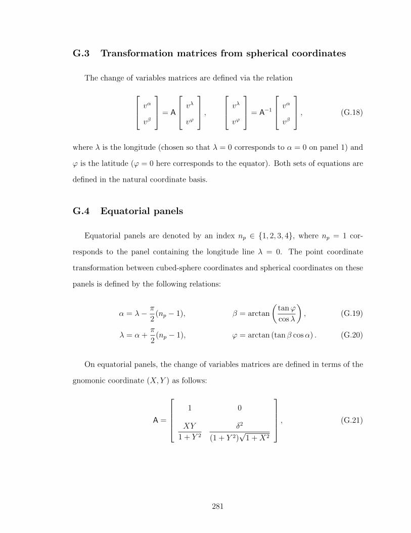
G.3 Transformation matrices from spherical coordinates

The change of variables matrices are defined via the relation

vα

vβ

= A

vλ

vϕ

, vλ

vϕ

= A−1

vα

vβ

, (G.18)

where λ is the longitude (chosen so that λ = 0 corresponds to α = 0 on panel 1) and

ϕ is the latitude (ϕ = 0 here corresponds to the equator). Both sets of equations are

defined in the natural coordinate basis.

G.4 Equatorial panels

Equatorial panels are denoted by an index np ∈ 1, 2, 3, 4, where np = 1 cor-

responds to the panel containing the longitude line λ = 0. The point coordinate

transformation between cubed-sphere coordinates and spherical coordinates on these

panels is defined by the following relations:

α = λ− π

2(np − 1), β = arctan

(tanϕ

cosλ

), (G.19)

λ = α +π

2(np − 1), ϕ = arctan (tan β cosα) . (G.20)

On equatorial panels, the change of variables matrices are defined in terms of the

gnomonic coordinate (X, Y ) as follows:

A =

1 0

XY

1 + Y 2

δ2

(1 + Y 2)√

1 +X2

, (G.21)

281

A−1 =

1 0

−XY√

1 +X2

δ2

(1 + Y 2)√

1 +X2

δ2

. (G.22)

G.4.0.1 Polar panels

Polar panels are denoted by an index np ∈ 5, 6 where the index p = 5 corre-

sponds to the north polar panel and the index np = 6 corresponds to the south polar

panel. We define a panel indicator s as

s =

1 if np = 5,

−1 if np = 6.(G.23)

The pointwise coordinate transforms then take the form:

α = s arctan (cotϕ sinλ) , β = − arctan (cotϕ cosλ) , (G.24)

λ = − arctan

(tanα

tan β

), ϕ = s arccot

(√tan2 α + tan2 β

). (G.25)

The pointwise change of variables matrices are defined by:

A =

−sY

1 +X2

−sδ2X

(1 +X2)√X2 + Y 2

sX

1 + Y 2

−sδ2Y

(1 + Y 2)√X2 + Y 2

. (G.26)

A−1 =

−sY (1 +X2)

X2 + Y 2

sX(1 + Y 2)

X2 + Y 2

− sX(1 +X2)

δ2√X2 + Y 2

− sY (1 + Y 2)

δ2√X2 + Y 2

. (G.27)

282

G.4.1 Coriolis source term

The Coriolis source terms of the momentum equation takes the form

ψC = −2Ω× (ρu), Ω = ω [cosϕeϕ + sinϕer] , (G.28)

at latitude ϕ and with latitudinal unit basis vector eϕ and radial basis vector er. In

terms of cubed-sphere coordinates, Ω is

Ω =

ω

δ

[1 +X2

r

[gα +

XY

1 + Y 2gβ

]+ Y gr

]for equatorial panels (np < 5),

sω

δ

[√X2 + Y 2

r

[−Y

1 +X2gα +

X

1 + Y 2gβ

]+ gr

]for polar panels (np ≥ 5)

(G.29)

283

APPENDIX H

The shallow-atmosphere approximation

The shallow-atmosphere approximation has the effect of reducing the vertically

varying structure of the atmosphere to a set of stacked layers. Layers are approxi-

mated to have radius r = a, which removes geometric terms associated with increas-

ing area as altitude increases. This approximation was first introduced by Phillips

(1966). It is described in conjuction with other consistent approximations of the full

non-hydrostatic primitive equations in White et al. (2005).

Following the metric formulation described in Appendix G, the shallow-atmosphere

approximation follows by simply replacing all instances of r in the deep-atmosphere

metric (G.1)-(G.2) with the radius of the Earth a. As a result, the infinitesmal volume

element becomes

J =√

detGij =a2(1 +X2)(1 + Y 2)

δ3, dV = Jdαdβdz, (H.1)

284

where z is the height above the orography. Infinitesmal areas along surfaces (G.6)-

(G.8) likewise become

Jα =a(1 + Y 2)

√1 +X2

δ2dAα = Jαdβdr, (H.2)

Jβ =a(1 +X2)

√1 + Y 2

δ2dAβ = Jβdαdr, (H.3)

Jr =a2(1 +X2)(1 + Y 2)

δ3dAr = Jrdαdβ. (H.4)

The Christoffel symbols are significantly affected by this change, now taking the form

Γα =

2XY 2

δ2

−Y (1 + Y 2)

δ20

−Y (1 + Y 2)

δ20 0

0 0 0

, (H.5)

Γβ =

0

−X(1 +X2)

δ20

−X(1 +X2)

δ2

2X2Y

δ20

0 0 0

, (H.6)

Γr = 0. (H.7)

Finally, conservation of energy requires that so-called “cosine Coriolis terms” be

dropped from the momentum evolution equation. As a consequence, all gα and gβ

dependence of (G.29) is dropped and (G.28) simplifies to

ψC = −fgr × (ρu), (H.8)

where

f =2ω

δ

Y for equatorial panels (np < 5)

s for polar panels (np ≥ 5)(H.9)

285

BIBLIOGRAPHY

286

BIBLIOGRAPHY

Adcroft, A., C. Hill, and J. Marshall (1997), Representation of Topography by ShavedCells in a Height Coordinate Ocean Model, Monthly Weather Review, 125, 2293–2315, doi:10.1175/1520-0493(1997)125〈2293:ROTBSC〉2.0.CO;2.

Adcroft, A., C. Hill, J. M. Campin, J. Marshall, and P. Heimbach (2004), Overviewof the Formulation and Numerics of the MIT GCM, in Proceedings of the ECMWFseminar series on Numerical Methods, Recent developments in numerical methodsfor atmosphere and ocean modelling., pp. 139–149, Reading, U.K., 6-10 September,2004.

Ahmad, N., and J. Lindeman (2007), Euler solutions using flux-based wave decom-position, Int. J. Num. Meth. Fluids, 54, 47–72, doi:10.1002/fld.1392.

Alaka, M. (1960), The airflow over mountains, WMO Tech. Note 34, 135 pp.

Alcrudo, F., and P. Garcia-Navarro (1993), A high-resolution Godunov-type schemein finite volumes for the 2D shallow-water equations, International Journal forNumerical Methods in Fluids, 16, 489–505, doi:10.1002/fld.1650160604.

Arakawa, A. (1970), Numerical Simulation of Large-Scale Atmospheric Motions, inNumerical Solution of Field Problems in Continuum Physics (SIAM-AMS Confer-ence), vol. 2, pp. 24–40, American Mathematical Society, Providence, RI.

Arakawa, A., and C. S. Konor (2009), Unification of the Anelastic and Quasi-Hydrostatic Systems of Equations, Monthly Weather Review, 137, 710–726, doi:10.1175/2008MWR2520.1.

Arakawa, A., and V. Lamb (1977), Computational design and the basic dynami-cal processes of the UCLA general circulation model, Methods in ComputationalPhysics, 17, 173–265.

Ascher, U., S. Ruuth, and R. Spiteri (1997), Implicit-explicit Runge-Kutta methodsfor time-dependent partial differential equations, Applied Numerical Mathematics,25 (2-3), 151–167, doi:10.1016/S0168-9274(97)00056-1.

Bale, D. S. (2002), Wave propagation algorithms on curved manifolds with applica-tions to relativistic hydrodynamics, Ph.D. thesis, University of Washington, 154pp.

287

Barad, M., and P. Colella (2005), A fourth-order accurate local refinement methodfor Poisson’s equation, Journal of Computational Physics, 209, 1–18, doi:10.1016/j.jcp.2005.02.027.

Barth, T., and D. Jespersen (1989), The design and application of upwind schemeson unstructured meshes, in Proc. AIAA 27th Aerospace Sciences Meeting, Reno,NV, January 9-12, 1989.

Berger, M. J., and P. Colella (1989), Local adaptive mesh refinement for shock hydro-dynamics, Journal of Computational Physics, 82, 64–84, doi:10.1016/0021-9991(89)90035-1.

Berger, M. J., and J. Oliger (1984), Adaptive Mesh Refinement for Hyperbolic Par-tial Differential Equations, Journal of Computational Physics, 53, 484–512, doi:10.1016/0021-9991(84)90073-1.

Bergthorsson, P., B. R. Doos, S. Fryklund, O. Haug, and R. Lindquist (1955), RoutineForecasting with the Barotropic Model, Tellus, 7, 272–76.

Black, T. L. (1994), The New NMC Mesoscale Eta Model: Description and Fore-cast Examples, Weather and Forecasting, 9, 265–284, doi:10.1175/1520-0434(1994)009〈0265:TNNMEM〉2.0.CO;2.

Bockman, S. (1989), Generalizing the formula for areas of polygons to moments,Amer. Math. Mon., 96 (2), 131–132.

Bonaventura, L. (2000), A semi-implicit semi-Lagrangian scheme using the height co-ordinate for a nonhydrostatic and fully elastic model of atmospheric flows, Journalof Computational Physics, 158, 186–213, doi:10.1006/jcph.1999.6414.

Bonaventura, L., and T. Ringler (2005), Analysis of Discrete Shallow-Water Modelson Geodesic Delaunay Grids with C-Type Staggering, Monthly Weather Review,133, 2351–2373, doi:10.1175/MWR2986.1.

Boris, J. P., and D. L. Book (1973), Flux-Corrected Transport. I. SHASTA, A FluidTransport Algorithm That Works, Journal of Computational Physics, 11, 38–69,doi:10.1016/0021-9991(73)90147-2.

Brillouin, L. (1960), Wave Propagation and Group Velocity, 154 pp., Academic Press(New York).

Cathers, B., and S. Bates (1995), Spurious numerical refraction, International Journalfor Numerical Methods in Fluids, 21, 1049–1066, doi:10.1002/fld.1650211104.

Charney, J. G., R. Fjørtoft, and J. von Neumann (1950), Numerical Integration ofthe Barotropic Vorticity Equation, Tellus, 2, 237–254.

Chen, C., and F. Xiao (2008), Shallow water model on cubed-sphere by multi-momentfinite volume method, Journal of Computational Physics, 227, 5019–5044, doi:10.1016/j.jcp.2008.01.033.

288

Chin, R. C. Y., and G. W. Hedstrom (1982), Scattering of Waves from a StaggeredDifference Scheme on a Variable Grid, in Proc. 10th IMACS World Congress, Mon-treal, Que., pp. 49–51, August 8-13, 1982.

Chung, T. J. (2002), Computational Fluid Dynamics, 1012 pp., Cambridge UniversityPress.

Colella, P., and P. R. Woodward (1984), The Piecewise Parabolic Method (PPM)for Gas-Dynamical Simulations, Journal of Computational Physics, 54, 174–201,doi:10.1016/0021-9991(84)90143-8.

Colella, P., et al. (2009), Chombo Software Package for AMR Applications DesignDocument, Tech. rep., Lawrence Berkeley National Laboratory.

Collins, W., et al. (2006), The Community Climate System Model version 3 (CCSM3),Journal of Climate, 19, 2122–2143.

Collins, W. D., P. J. Rasch, B. A. Boville, J. J. Hack, J. R. McCaa, D. L. Williamson,J. T. Kiehl, and B. Briegleb (2004), Description of the NCAR Community Atmo-sphere Model (CAM 3.0). NCAR Tech. Note, NCAR/TN-464+STR.

Cote, J., and A. Staniforth (1990), An accurate and efficient finite-element globalmodel of the shallow-water equations, Monthly Weather Review, 118, 2707–2717.

Cote, J., S. Gravel, A. Methot, A. Patoine, M. Roch, and A. Staniforth (1998), TheOperational CMC MRB Global Environmental Multiscale (GEM) Model. Part I:Design Considerations and Formulation, Monthly Weather Review, 126, 1373–1395,doi:10.1175/1520-0493(1998)126〈1373:TOCMGE〉2.0.CO;2.

Courant, R., K. Friedrichs, and H. Lewy (1928), Uber die partiellen Differenzen-gleichungen der mathematischen Physik, Mathematische Annalen, 100 (1), 32–74.

Crouzeix, M. (1980), Une methode multipas implicite-explicite pour l’approximationdes equations d’evolution paraboliques, Numerische Mathematik, 35, 257–276, doi:10.1007/BF01396412.

Davies, T., A. Staniforth, N. Wood, and J. Thuburn (2003), Validity of anelastic andother equation sets as inferred from normal-mode analysis, Quart. J. Royal Meteor.Soc., 129, 2761–2775, doi:10.1256/qj.02.1951.

Davies, T., M. J. P. Cullen, A. J. Malcolm, M. H. Mawson, A. Staniforth, A. A.White, and N. Wood (2005), A new dynamical core for the Met Office’s globaland regional modelling of the atmosphere, Quart. J. Royal Meteor. Soc., 131 (608),1759–1782, doi:10.1256/qj.04.101.

Dennis, J., J. Edwards, K. J. Evans, O. Guba, P. H. Lauritzen, A. A. Mirin, A. St-Cyr, M. A. Taylor, and P. H. Worley (2011), CAM-SE: A scalable spectral elementdynamical core for the community atmosphere model, Int. J. High. Perform. C.Appl., submitted.

289

Dukowicz, J. K., and J. W. Kodis (1987), Accurate conservative remapping (rezoning)for arbitrary Lagrangian-Eulerian computations, SIAM J. Sci. Stat. Comput., 8 (3),305–321, doi:http://dx.doi.org/10.1137/0908037.

Durran, D. R. (1989), Improving the anelastic approximation., Journal of the Atmo-spheric Sciences, 46, 1453–1461, doi:10.1175/1520-0469(1989)046〈1453:ITAA〉2.0.CO;2.

Durran, D. R. (1999), Numerical methods for wave equations in geophysical fluiddynamics, 489 pp., Springer-Verlag.

Durran, D. R., and J. B. Klemp (1982), The effects of moisture on trapped mountainlee waves, Journal of the Atmospheric Sciences, 39 (11), 2490–2506, doi:10.1175/1520-0469(1982)039〈2490:TEOMOT〉2.0.CO;2.

Edwards, P. N. (2010), A Vast Machine: Computer Models, Climate Data, and thePolitics of Global Warming, 528 pp., MIT Press.

Fels, S. B., J. D. Mahlman, M. D. Schwarzkopf, and R. W. Sinclair (1980), Strato-spheric Sensitivity to Perturbations in Ozone and Carbon Dioxide: Radiativeand Dynamical Response., Journal of Atmospheric Sciences, 37, 2265–2297, doi:10.1175/1520-0469(1980)037〈2265:SSTPIO〉2.0.CO;2.

Fournier, A., M. A. Taylor, and J. J. Tribbia (2004), The spectral element atmo-sphere model (SEAM): High-resolution parallel computation and localized res-olution of regional dynamics, Monthly Weather Review, 132 (3), 726–748, doi:10.1175/1520-0493(2004)132〈0726:TSEAMS〉2.0.CO;2.

Fox-Rabinovitz, M., J. Cote, B. Dugas, M. Deque, and J. L. McGregor (2006), Vari-able resolution general circulation models: Stretched-grid model intercomparisonproject (SGMIP), Journal of Geophysical Research (Atmospheres), 111, 16,104–16,124, doi:10.1029/2005JD006520.

Fox-Rabinovitz, M. S. (1991), Computational Dispersion Properties of HorizontalStaggered Grids for Atmospheric and Ocean Models, Monthly Weather Review,119, 1624–1639, doi:10.1175/1520-0493(1991)119〈1624:CDPOHS〉2.0.CO;2.

Fox-Rabinovitz, M. S., G. L. Stenchikov, M. J. Suarez, and L. L. Takacs (1997), AFinite-Difference GCM Dynamical Core with a Variable-Resolution Stretched Grid,Monthly Weather Review, 125, 2943–2968, doi:10.1175/1520-0493(1997)125〈2943:AFDGDC〉2.0.CO;2.

Fox-Rabinovitz, M. S., L. L. Takacs, R. C. Govindaraju, and M. J. Suarez (2001), AVariable-Resolution Stretched-Grid General Circulation Model: Regional ClimateSimulation, Monthly Weather Review, 129, 453–469, doi:10.1175/1520-0493(2001)129〈0453:AVRSGG〉2.0.CO;2.

290

Frank, J., and S. Reich (2004), On Spurious Reflections, Non-uniform Grids and FiniteDifference Discretizations of Wave Equations, Tech. rep., Center for Mathematicsand Computer Science, CWI Report MAS-E0406.

Fromm, J. E. (1968), A Method for Reducing Dispersion in Convective DifferenceSchemes, Journal of Computational Physics, 3, 176–189, doi:10.1016/0021-9991(68)90015-6.

Gadd, A. J. (1978), A split explicit integration scheme for numerical weather predic-tion, Quart. J. Roy. Meteor. Soc., 104, 569–582, doi:10.1002/qj.49710444103.

Gal-Chen, T., and R. C. J. Somerville (1975), On the use of a coordinate transfor-mation for the solution of the Navier-Stokes equations, Journal of ComputationalPhysics, 17, 209–228, doi:10.1016/0021-9991(75)90037-6.

Galewsky, J., R. K. Scott, and L. M. Polvani (2004), An initial-value problem fortesting numerical models of the global shallow-water equations, Tellus Series A,56, 429–440, doi:10.1111/j.1600-0870.2006.00192.x.

Gaßmann, A. (2010), Non-hydrostatic modelling with the ICON model, Presentationat ECMWF Non-Hydrostatic Workshop, Reading, U.K., Nov. 8-10, 2010.

Giraldo, F. X., and M. Restelli (2008), A study of spectral element and discontinuousGalerkin methods for the Navier Stokes equations in nonhydrostatic mesoscaleatmospheric modeling: Equation sets and test cases, Journal of ComputationalPhysics, 227, 3849–3877, doi:10.1016/j.jcp.2007.12.009.

Giraldo, F. X., and T. E. Rosmond (2004), A Scalable Spectral Element EulerianAtmospheric Model (SEE-AM) for NWP: Dynamical Core Tests, Monthly WeatherReview, 132, 133–153, doi:10.1175/1520-0493(2004)132〈0133:ASSEEA〉2.0.CO;2.

Giraldo, F. X., J. S. Hesthaven, and T. Wartburton (2002), Nodal high-order discon-tinous galerkin methods for the shallow water equations, Journal of ComputationalPhysics, 181, 499–525.

Godunov, S. K. (1959), A difference scheme for numerical solution of discontinuoussolution of hydrodynamic equations, Math. Sbornik, 47, 271–306, translated USJoint Publ. Res. Service, JPRS 7226, 1969.

Gottlieb, S., C.-W. Shu, and E. Tadmor (2001), Strong stability-preserving high-order time discretization methods, SIAM Review, 43 (1), 89–112, doi:10.1137/S003614450036757X.

Govett, M. W., J. Middlecoff, and T. Henderson (2010), Running the NIM next-generation weather model on GPUs, Cluster Computing and the Grid, IEEE In-ternational Symposium on, 0, 792–796, doi:10.1109/CCGRID.2010.106.

291

Grotjahn, R., and J. J. O’Brien (1976), Some Inaccuracies in Finite Differenc-ing Hyperbolic Equations, Monthly Weather Review, 104, 180–194, doi:10.1175/1520-0493(1976)104〈0180:SIIFDH〉2.0.CO;2.

Guillard, H., and C. Viozat (1999), On the behaviour of upwind schemes in the lowmach number limit, Comput. Fluids, 28, 63–86.

Hack, J. J., et al. (2008), Report on computational and informational technology ratelimiters to the advancement of climate change science, Tech. rep., Advanced Scien-tific Computing Advisory Committee and Biological and Environmental AdvisoryCommittee, Department of Energy.

Harper, K. C. (2008), Weather by the Numbers: The Genesis of Modern Meteorology,328 pp., MIT Press, Cambridge, MA.

Harten, A., P. Lax, and B. van Leer (1983), On Upstream Differencing and Godunov-Type Schemes for Hyperbolic Conservation Laws, SIAM Review, 25 (1), 35–61.

Haurwitz, B. (1940), The motion of atmospheric disturbances on the spherical earth,Journal of Marine Research, 3, 254–267.

Heikes, R., and D. A. Randall (1995), Numerical integration of the shallow waterequations on a twisted icosahedral grid. Part I: Basic design and results of tests,Monthly Weather Review, 123, 1862–1880.

Henderson, T. B., S. Benjamin, R. Bleck, J. Brown, S. Sun, J. Bao, S. Sahm, G. A.Grell, and M. Fiorino (2010), Progress in development of the Flow-following finite-volume Icosahedral Model (FIM) toward improving NCEP global ensemble fore-casts and toward a chemistry-coupled global, AGU Fall Meeting Abstracts, pp.A41B–0088.

Jablonowski, C., and D. L. Williamson (2006), A baroclinic instabilitiy test casefor atmospheric model dynamical cores, Quart. J. Roy. Meteor. Soc., 132 (621C),2943–2975.

Jablonowski, C., M. Herzog, J. E. Penner, R. C. Oehmke, Q. F. Stout, B. vanLeer, and K. G. Powell (2006), Block-Structured Adaptive Grids on the Sphere:Advection Experiments, Monthly Weather Review, 134, 3691–3713, doi:10.1175/MWR3223.1.

Jablonowski, C., P. H. Lauritzen, M. A. Taylor, and R. D. Nair (2008a), An Intercom-parison of 10 Atmospheric Model Dynamical Cores, in Eos Trans. AGU, 89(53),Fall Meet. Suppl., Abstract A33A-0214.

Jablonowski, C., P. H. Lauritzen, M. A. Taylor, and R. D. Nair (2008b), Idealizedtest cases for the dynamical cores of Atmospheric General Circulation Models: Aproposal for the NCAR ASP 2008 summer colloquium, Tech. rep., NCAR, availableat http://esse.engin.umich.edu/admg/publications.php.

292

Jablonowski, C., R. C. Oehmke, and Q. F. Stout (2009), Block-structured Adap-tive Meshes and Reduced Grids for Atmospheric General Circulation Models, Phil.Trans. R. Soc. A, 367, 4497–4522.

Jablonowski, C., P. Ullrich, F. Giraldo, J. Kelly, T. Hundertmark, and S. Reich(2011), The baroclinic instability in a channel: A test case for atmospheric limitedarea models, in preparation.

Jakob-Chien, R., J. J. Hack, and D. L. Williamson (1995), Spectral transform solu-tions to the shallow water test set, Journal of Computational Physics, 119, 164–187.

Jebens, S., O. Knoth, and R. Weiner (2010), Linearly implicit peer methods for thecompressible Euler equations, Journal of Computational Physics, in press.

Jones, P. W. (1999), First- and second-order conservative remapping schemes for gridsin spherical coordinates, Monthly Weather Review, 127, 2204–2210.

Karni, S. (1994), On the group velocity of symmetric and upwind numerical schemes,International Journal for Numerical Methods in Fluids, 18, 1073–1081, doi:10.1002/fld.1650181105.

Kasahara, A. (1974), Various Vertical Coordinate Systems Used for Numeri-cal Weather Prediction, Monthly Weather Review, 102, 509–522, doi:10.1175/1520-0493(1974)102〈0509:VVCSUF〉2.0.CO;2.

Kasahara, A., and W. M. Washington (1967), NCAR Global General CirculationModel of the Atmosphere, Monthly Weather Review, 95, 389–402, doi:10.1175/1520-0493(1967)095.

Keller, T. L. (1994), Implications of the Hydrostatic Assumption on AtmosphericGravity Waves., Journal of Atmospheric Sciences, 51, 1915–1929, doi:10.1175/1520-0469(1994)051〈1915:IOTHAO〉2.0.CO;2.

Kurihara, Y. (1965), Numerical Integration of the Primitive Equations on a Spher-ical Grid, Monthly Weather Review, 93, 399–415, doi:10.1175/1520-0493(1965)093〈0399:NIOTPE〉2.3.CO;2.

Kwizak, M., and A. J. Robert (1971), A semi-implicit scheme for grid point atmo-spheric models of the primitive equations, Monthly Weather Review, 99, 32–36,doi:10.1175/1520-0493(1971)099〈0032:ASSFGP〉2.3.CO;2.

Laprise, J. P. R., and A. Plante (1995), A Class of Semi-Lagrangian Integrated-Mass(SLIM) Numerical Transport Algorithms, Monthly Weather Review, 123, 553–565,doi:10.1175/1520-0493(1995)123〈0553:ACOSLI〉2.0.CO;2.

Lauritzen, P. H., and R. D. Nair (2007), Monotone and conservative cascade remap-ping between spherical grids (CaRS): Regular latitude-longitude and cubed-spheregrids, Monthly Weather Review, 136, 1416–1432.

293

Lauritzen, P. H., P. A. Ullrich, and R. D. Nair (2008), A finite-volume multi-tracer transport/advection scheme on the cubed sphere, Journal of ComputationalPhysics, in prep.

Lauritzen, P. H., C. Jablonowski, M. A. Taylor, and R. D. Nair (2010), Rotated ver-sions of the Jablonowski steady-state and baroclinic wave test cases: A dynamicalcore intercomparison, J. Adv. Model. Earth Syst., 2, doi:10.3894/JAMES.2010.2.15,art. #15, 34 pp.

Lauritzen, P. H., R. D. Nair, and P. A. Ullrich (2010), A conservative semi-Lagrangianmulti-tracer transport scheme (CSLAM) on the cubed-sphere grid., Journal ofComputational Physics, 229, 1401–1424.

Lax, P., and B. Wendroff (1960), Systems of conservation laws, Communications onPure and Applied Mathematics, 13 (2), 217–237, doi:10.1002/cpa.3160130205.

Lax, P. D. (1954), Weak solutions of non-linear hyperbolic equations and their nu-merical computation, Comm. Pure Appl. Math., VII, 159–193.

Lee, J., R. Bleck, A. E. MacDonald, J. Bao, and S. Benjamin (2006), A flow-followingfinite-volume icosahedral model, Eos Trans. AGU, 87 (52), Fall Meet. Suppl., Ab-stract A33F–04.

LeVeque, R. (1997), Wave propagation algorithms for multidimensional hyperbolicsystems, Journal of Computational Physics, 131, 327–353, doi:10.1006/jcph.1996.5603.

Lin, S.-J. (2004), A “Vertically Lagrangian” Finite-Volume Dynamical Core for GlobalModels, Monthly Weather Review, 132, 2293–2307, doi:10.1175/1520-0493(2004)132〈2293:AVLFDC〉2.0.CO;2.

Lin, S.-J., and R. B. Rood (1996), Multidimensional flux-form semi-Lagrangian trans-port schemes, Monthly Weather Review, 124, 2046–2070.

Lin, S.-J., and R. B. Rood (1997), An explicit flux-form semi-Lagrangian shallow-water model on the sphere, Quart. J. Royal Meteor. Soc., 123, 2477–2498, doi:10.1256/smsqj.54415.

Liou, M.-S. (2006), A sequel to AUSM, Part II: AUSM+-up for all speeds, Journalof Computational Physics, 214, 137–170, doi:10.1016/j.jcp.2005.09.020.

Liou, M.-S., and C. Steffen (1993), A new flux splitting scheme, Journal of Compu-tational Physics, 107, 23–39.

Liu, Y., C. Shu, E. Tadmor, and M. Zhang (2007), Central discontinuous Galerkinmethods on overlapping cells with a non-oscillatory hierarchical reconstruction,SIAM J. Numer. Anal, 45, 2442–2467.

294

Long, D. (2009), Spurious propagation of hyperbolic waves on in-homogeneously stag-gered grids, Master’s thesis, University of Exeter, U.K.

Long, D., and J. Thuburn (2011), Numerical wave propagation on non-uniform one-dimensional staggered grids, Journal of Computational Physics, 230, 2643–2659,doi:10.1016/j.jcp.2010.12.040.

Lorenz, E. N. (1963), Deterministic Nonperiodic Flow, Journal of Atmospheric Sci-ences, 20, 130–148, doi:10.1175/1520-0469(1963)020〈0130:DNF〉2.0.CO;2.

MacCormack, R. (2003), The Effect of Viscosity in Hypervelocity Impact Cratering,Journal of Spacecraft and Rockets, 40, 757–763, doi:10.2514/2.6901.

Majewski, D. (1998), The new global icosahedral-hexagonal gridpoint model GME ofthe Deutscher Wetterdienst., in Proc. Seminar on Numerical Methods for WeatherPrediction, vol. 1, pp. 172–201, ECMWF, Reading, United Kingdom.

Majewski, D., D. Liermann, P. Prohl, B. Ritter, M. Buchhold, T. Hanisch, G. Paul,W. Wergen, and J. Baumgardner (2002), The Operational Global IcosahedralHexagonal Gridpoint Model GME: Description and High-Resolution Tests, MonthlyWeather Review, 130, 319–338, doi:10.1175/1520-0493(2002)130〈0319:TOGIHG〉2.0.CO;2.

Manabe, S., and J. Smagorinsky (1965), Simulated Climatology of General Circula-tion with a Hydrologic Cycle, Monthly Weather Review, 93, 769–798.

Margolin, L. G., and M. Shashkov (2003), Second-order sign-preserving conservativeinterpolation (remapping) on general grids, Journal of Computational Physics, 184,266–298.

Marshall, J., A. Adcroft, C. Hill, L. Perelman, and C. Heisey (1997), A finite-volume,incompressible Navier Stokes model for studies of the ocean on parallel computers,Journal of Geophysical Research, 102, 5753–5766, doi:10.1029/96JC02775.

Mintz, Y. (1965), Very Long-Term Global Integration of the Primitive Equations ofAtmospheric Motion, in WMO-IUGG Symposium on Research and DevelopmentAspects of Long-Range Forecasting, Boulder, Colo., 1964. (WMO Technical NoteNo. 66), edited by W. M. Organization.

Nair, R. D., and B. Machenhauer (2002), The mass-conservative cell-integrated semi-Lagrangian advection scheme on the sphere, Monthly Weather Review, 130 (3),649–667.

Nair, R. D., S. J. Thomas, and R. D. Loft (2005), A discontinuous Galerkin transportscheme on the cubed sphere, Monthly Weather Review, 133, 814–828.

Nair, R. D., S. J. Thomas, and R. D. Loft (2005), A discontinuous Galerkinglobal shallow water model, Monthly Weather Review, 133, 876–888, doi:10.1175/MWR2903.1.

295

National Academy of Sciences (1966), Weather and Climate Modification: Problemsand Prospects (2 Vols.), National Academy of Sciences, Washington, DC, Commit-tee on Atmospheric Sciences Panel on Weather and Climate Modification.

Noelle, S., N. Pankratz, G. Puppo, and J. R. Natvig (2006), Well-balanced finitevolume schemes of arbitrary order of accuracy for shallow water flows, Journal ofComputational Physics, 213, 474–499, doi:10.1016/j.jcp.2005.08.019.

Nørsett, S. P., and A. Wolfbrandt (1979), Order conditions for Rosenbrock typemethods, Numerische Mathematik, 32, 1–15, 10.1007/BF01397646.

Ogura, Y., and N. A. Phillips (1962), Scale analysis of deep and shallow convection inthe atmosphere., Journal of the Atmospheric Sciences, 19, 173–179, doi:10.1175/1520-0469(1962)019.

Osher, S., and J. A. Sethian (1988), Fronts Propagating with Curvature-DependentSpeed: Algorithms Based on Hamilton-Jacobi Formulations, Journal of Computa-tional Physics, 79, 12–49, doi:10.1016/0021-9991(88)90002-2.

Phillips, N. A. (1956), The General Circulation of the Atmosphere: A NumericalExperiment, Quart. J. Roy. Met. Soc., 82, 123–64.

Phillips, N. A. (1957), A Coordinate System Having Some Special Advantages forNumerical Forecasting., Journal of the Atmospheric Sciences, 14, 184–185, doi:10.1175/1520-0469(1957)014〈0184:ACSHSS〉2.0.CO;2.

Phillips, N. A. (1966), The Equations of Motion for a Shallow Rotating Atmosphereand the ‘Traditional Approximation’, Journal of Atmospheric Sciences, 23, 626–627, doi:10.1175/1520-0469(1966)023〈0626:TEOMFA〉2.0.CO;2.

Prather, M. J. (1986), Numerical advection by conservation of second-order moments,Journal of Geophysical Research, 91, 6671–6681, doi:10.1029/JD091iD06p06671.

Putman, W. M., and S.-J. Lin (2007), Finite-volume transport on various cubed-sphere grids, Journal of Computational Physics, 227, 55–78, doi:10.1016/j.jcp.2007.07.022.

Putman, W. M., and S.-J. Lin (2009), A finite-volume dynamical core on the cubed-sphere grid, in Numerical Modeling of Space Plasma Flows: Astronum-2008, vol.406, edited by N. V. Pogorelov, E. Audit, P. Colella, and G. P. Zank, pp. 268–276,Astronomical Society of the Pacific Conference Series.

Putman, W. M., and M. Suarez (2009), Mesoscale weather and climate modeling withthe global non-hydrostatic Goddard Earth Observing System Model (GEOS-5) atcloud-permitting resolutions, AGU Fall Meeting Abstracts, abs. # A42B-08.

Randall, D. A. (1994), Geostrophic Adjustment and the Finite-Difference Shallow-Water Equations, Monthly Weather Review, 122, 1371–1377, doi:10.1175/1520-0493(1994)122〈1371:GAATFD〉2.0.CO;2.

296

Randall, D. A. (2000), General Circulation Model development: Past, present, andfuture, Academic Press, 807 pp.

Rancic, M. (1992), Semi-Lagrangian piecewise biparabolic scheme for two-dimensionalhorizontal advection of a passive scalar, Monthly Weather Review, 120, 1394–1405.

Rancic, M., J. Purser, and F. Mesinger (1996), A global shallow water model usingan expanded spherical cube, Quart. J. Roy. Meteor. Soc., 122, 959–982.

Restelli, M., and F. X. Giraldo (2009), A conservative discontinuous Galerkin semi-implicit formulation for the Navier-Stokes equations in nonhydrostatic mesoscalemodeling, SIAM Journal of Scientific Computing, 31 (3), 2231–2257, doi:10.1137/070708470.

Richardson, L. F. (1922), Weather Prediction by Numerical Process, 250 pp., Cam-bridge University Press, Cambridge, MA, reprinted NY, Dover, 1965.

Ringler, T. D., R. P. Heikes, and D. A. Randall (2000), Modeling the AtmosphericGeneral Circulation Using a Spherical Geodesic Grid: A New Class of Dynami-cal Cores, Monthly Weather Review, 128, 2471–2490, doi:10.1175/1520-0493(2000)128〈2471:MTAGCU〉2.0.CO;2.

Robert, A. (1993), Bubble convection experiments with a semi-implicit formulationof the Euler equations, Journal of the Atmospheric Sciences, 50, 1865–1873, doi:10.1175/1520-0469(1993)050〈1865:BCEWAS〉2.0.CO;2.

Roe, P. L. (1981), Approximate Riemann solvers, parameter vectors, and dif-ference schemes, Journal of Computational Physics, 43, 357–372, doi:10.1016/0021-9991(81)90128-5.

Ronchi, C., R. Iacono, and P. S. Paolucci (1996), The “cubed sphere”: A new methodfor the solution of partial differential equations in spherical geometry, Journal ofComputational Physics, 124 (1), 93–114.

Rood, R. B. (1987), Numerical advection algorithms and their role in atmospherictransport and chemistry models, Reviews of Geophysics, 25, 71–100, doi:10.1029/RG025i001p00071.

Rosenbrock, H. (1963), Some general implicit processes for the numerical solution ofdifferential equations., The Computer Journal, 5, 329–330.

Rossmanith, J. A. (2006), A wave propagation method for hyperbolic systems on thesphere, Journal of Computational Physics, 213, 629–658, doi:10.1016/j.jcp.2005.08.027.

Rusanov, V. V. (1961), Calculation of intersection of non-steady shock waves withobstacles, J. Comput. Math. Phys. USSR, 1, 267–279.

297

Sadourny, R. (1972), Conservative finite-difference approximations of the primitiveequations on quasi-uniform spherical grids, Monthly Weather Review, 100, 136–144.

Sadourny, R., A. Arakawa, and Y. Mintz (1968), Integration of the nondivergentbarotropic vorticity equation with an icosahedral-hexagonal grid for the sphere,Monthly Weather Review, 96, 351–356, doi:10.1175/1520-0493(1968)096〈0351:IOTNBV〉2.0.CO;2.

Schmidt, G. A., et al. (2006), Present-Day Atmospheric Simulations Using GISS Mod-elE: Comparison to In Situ, Satellite, and Reanalysis Data., Journal of Climate,19, 153–192, doi:10.1175/JCLI3612.1.

Simmons, A. J., and D. M. Burridge (1981), An energy and angular-momentumconserving vertical finite-difference scheme and hybrid vertical coordinates, Mon.Wea. Rev., 109, 758–766.

Skamarock, W. C., and J. B. Klemp (1993), Adaptive Grid Refinement for Two-Dimensional and Three-Dimensional Nonhydrostatic Atmospheric Flow, MonthlyWeather Review, 121, 788–804, doi:10.1175/1520-0493(1993)121〈0788:AGRFTD〉2.0.CO;2.

Skamarock, W. C., and J. B. Klemp (2008), A time-split nonhydrostatic atmosphericmodel for weather research and forecasting applications, Journal of ComputationalPhysics, 227, 3465–3485, doi:10.1016/j.jcp.2007.01.037.

Skamarock, W. C., J. Oliger, and R. L. Street (1989), Adaptive Grid Refinementfor Numerical Weather Prediction, Journal of Computational Physics, 80, 27–60,doi:10.1016/0021-9991(89)90089-2.

Skamarock, W. C., J. Klemp, M. Duda, S.-H. Park, L. Fowler, T. Ringler, J. Thuburn,M. Gunzburger, and L. Ju (2010), Global Non-Hydrostatic Modeling Using VoronoiMeshes: The MPAS Model, Presentation at ECMWF Non-Hydrostatic Workshop,Reading, U.K. Nov. 8-10, 2010.

Smagorinsky, J. (1983), The Beginnings of Numerical Weather Prediction and Gen-eral Circulation Modeling: Early Recollections, Advances in Geophysics, 25, 3–37.

St-Cyr, A., C. Jablonowski, J. M. Dennis, H. M. Tufo, and S. J. Thomas (2008),A comparison of two shallow-water models with nonconforming adaptive grids,Monthly Weather Review, 136, 1898–1922, doi:10.1175/2007MWR2108.1.

Staniforth, A., and N. Wood (2008), Aspects of the dynamical core of a nonhydro-static, deep-atmosphere, unified weather and climate-prediction model, Journal ofComputational Physics, 227, 3445–3464, doi:10.1016/j.jcp.2006.11.009.

Staniforth, A. N., and H. L. Mitchell (1978), A Variable-Resolution Finite-ElementTechnique for Regional Forecasting with the Primitive Equations, Monthly WeatherReview, 106, 439–447, doi:10.1175/1520-0493(1978)106〈0439:AVRFET〉2.0.CO;2.

298

Taylor, M., J. Tribbia, and M. Iskandarani (1997), The spectral element method forthe shallow water equations on the sphere, Journal of Computational Physics, 130,92–108.

Taylor, M. A., J. Edwards, and A. St.Cyr (2008), Petascale atmospheric models forthe community climate system model: New developments and evaluation of scalabledynamical cores, J. Phys. Conf. Ser., 125, 012,023, doi:10.1088/1742-6596/125/1/012023.

Thomas, S. J., and R. D. Loft (2002), Semi-implicit spectral element atmo-spheric model, Journal of Scientific Computing, 17, 339–350, doi:10.1023/A:1015129420882.

Thomas, S. J., and R. D. Loft (2005), The NCAR spectral element climate dynamicalcore: Semi-implicit Eulerian formulation, Journal of Scientific Computing, 25 (1),307–322, doi:http://dx.doi.org/10.1007/s10915-004-4646-2.

Thuburn, J., and Y. Li (2000), Numerical simulations of Rossby Haurwitz waves,Tellus Series A, 52, 181–189, doi:10.1034/j.1600-0870.2000.00107.x.

Thuburn, J., T. D. Ringler, W. C. Skamarock, and J. B. Klemp (2009), Numericalrepresentation of geostrophic modes on arbitrarily structured C-grids, Journal ofComputational Physics, 228 (22), 8321–8335, doi:10.1016/j.jcp.2009.08.006.

Tomita, H., and M. Satoh (2004), A new dynamical framework of nonhydrostaticglobal model using the icosahedral grid, Fluid Dynamics Research, 34 (6), 357 –400, doi:10.1016/j.fluiddyn.2004.03.003.

Tomita, H., M. Tsugawa, M. Satoh, and K. Goto (2001), Shallow water model on amodified icosahedral geodesic grid by using spring dynamics, Journal of Computa-tional Physics, 174, 579–613, doi:10.1006/jcph.2001.6897.

Toro, E. F. (1999), Riemann Solvers and Numerical Methods for Fluid Dynamics,Second ed., 624 pp., Springer, ISBN-10: 3540659668.

Trefethen, L. N. (1982), Group velocity in finite difference schemes, SIAM Review,24 (2), 113–136, doi:10.1137/1024038.

Ullrich, P., and C. Jablonowski (2011a), Operator-Split Runge-Kutta-Rosenbrock(RKR) Methods for Non-hydrostatic Atmospheric Models, Monthly Weather Re-view, in review.

Ullrich, P. A., and C. Jablonowski (2011b), An analysis of 1D finite-volume methodsfor geophysical problems on refined grids, Journal of Computational Physics, 230,706–725, doi:10.1016/j.jcp.2010.10.014.

Ullrich, P. A., P. H. Lauritzen, and C. Jablonowski (2009), Geometrically exactconservative remapping (GECoRe): Regular latitude-longitude and cubed-spheregrids, Monthly Weather Review, 137, 1721–1741.

299

Ullrich, P. A., C. J. Jablonowski, and B. L. van Leer (2010), High-order finite-volumemodels for the shallow-water equations on the sphere, Journal of ComputationalPhysics, 229, 6104–6134.

van Leer, B. (1974), Towards the Ultimate Conservation Difference Scheme. II. Mono-tonicity and Conservation Combined in a Second-Order Scheme, Journal of Com-putational Physics, 14, 361–370, doi:10.1016/0021-9991(74)90019-9.

van Leer, B. (1977), Towards the Ultimate Conservative Difference Scheme. IV. ANew Approach to Numerical Convection, Journal of Computational Physics, 23,276–299, doi:10.1016/0021-9991(77)90095-X.

van Leer, B. (1979), Towards the ultimate conservative difference scheme. V - Asecond-order sequel to Godunov’s method, Journal of Computational Physics, 32,101–136, doi:10.1016/0021-9991(79)90145-1.

van Leer, B., J. Thomas, P. Roe, and R. Newsome (1987), A Comparison of NumericalFlux Formulas for the Euler and Navier-Stokes Equations, AIAA Paper No. 87-1104-CP, Computational Fluid Dynamics Conference, 8th, Honolulu, HI, June 9-11, 1987.

Varah, J. M. (1980), Stability restrictions on second order, three level finite differenceschemes for parabolic equations, SIAM J. Numer. Anal., 17 (2), 300–309, doi:10.1137/0717025.

Vichnevetsky, R. (1987), Wave propagation and reflection in irregular grids for hy-perbolic equations, Applied Numerical Mathematics, 3, 133–166.

Vichnevetsky, R., and L. H. Turner (1991), Spurious scattering from discontinuouslystretching grids in computational fluid dynamics, Applied Numerical Mathematics,8 (3), 289–299, doi:http://dx.doi.org/10.1016/0168-9274(91)90058-8.

Walko, R. L., and R. Avissar (2008), The Ocean-Land-Atmosphere Model (OLAM).Part II: Formulation and Tests of the Nonhydrostatic Dynamic Core, MonthlyWeather Review, 136, 4045–4062, doi:10.1175/2008MWR2523.1.

Wan, H. (2009), Developing and testing a hydrostatic atmospheric dynamical coreon triangular grids, Tech. Rep. 65, Reports on Earth System Science, Max-PlanckInstitute for Meteorology, Hamburg, Germany, iSSN 1614-119.

Washington, W., D. B. Bader, B. Collins, J. Drake, M. A. Taylor, B. Kirtman,D. N. Williams, and D. Middleton (2008), Challenges in climate change scienceand the role of computing at the extreme scale, Tech. rep., U.S. Department ofEnergy, Office of Biological and Environmental Research and the Office of AdvancedScientific Computing Research, Nov. 6-7, 2008, Washington D.C.

300

Wedi, N., P. Benard, K. Yessad, A. Untch, S. Malardel, M. Hamrud, G. Mozdzynski,M. Fisher, and P. Smolarkiewicz (2010), Non-hydrostatic modeling with IFS: cur-rent status, Presentation at ECMWF Non-Hydrostatic Workshop, Reading, U.K.,Nov. 8-10, 2010.

White, A. A., B. J. Hoskins, I. Roulstone, and A. Staniforth (2005), Consistentapproximate models of the global atmosphere: shallow, deep, hydrostatic, quasi-hydrostatic and non-hydrostatic, Quart. J. Royal Meteor. Soc., 131, 2081–2107,doi:10.1256/qj.04.49.

Williamson, D., J. Drake, J. Hack, R. Jakob, and P. Swarztrauber (1992), A standardtest set for numerical approximations to the shallow water equations in sphericalgeometry, Journal of Computational Physics, 102, 211–224.

Williamson, D. L. (1968), Integration of the barotropic vorticity equation on a spher-ical geodesic grid, Tellus, 20 (4), 642–653, doi:10.1111/j.2153-3490.1968.tb00406.x.

Williamson, D. L. (2008), Equivalent finite volume and Eulerian spectral transformhorizontal resolutions established from aqua-planet simulations, Tellus Series A,60, 839–847, doi:10.1111/j.1600-0870.2008.00340.x.

Wood, N., and A. Staniforth (2003), The deep-atmosphere Euler equations with amass-based vertical coordinate, Quart. J. Royal Meteor. Soc., 129, 1289–1300, doi:10.1256/qj.02.153.

Yeh, K., J. Cote, S. Gravel, A. Methot, A. Patoine, M. Roch, and A. Staniforth(2002), The CMC MRB Global Environmental Multiscale (GEM) Model. Part III:Nonhydrostatic Formulation, Monthly Weather Review, 130, 339–356, doi:10.1175/1520-0493(2002)130〈0339:TCMGEM〉2.0.CO;2.

Zalesak, S. T. (1979), Fully multidimensional flux-corrected transport algorithms forfluids, Journal of Computational Physics, 31, 335–362.

Zerroukat, M., N. Wood, and A. Staniforth (2005), A monotonic and positive-definitefilter for a semi-Lagrangian inherently conserving and efficient (SLICE) scheme,Quart. J. Royal Meteor. Soc., 131 (611), 2923–2936.

301