Atomic Force Microscopy on biological samples

Karls-Ruprecht Universität HeidelbergKirchhof-Institut für Physik - 2.208Im Neuenheimer Feld 227D-69120 Heidelberg

Betreuer: G.L. HeuvelmanKIP-2.19Tel: 06221 54 9268E-mail: Gerrit.Heuvelman@kip.uni-heidelberg.de

K. RippeKIP-3.19Tel: 06221 54 9270E-mail: Karsten.Rippe@kip.uni-heidelberg.de

F-2 Praktikum BiophysikWintersemester 2004/2005

Technical supportStart-up1. Turn on the computer and scanner by the power button behind the screen2. Open the program ‘nanoscope III 5.12r3’ and turn the microscope button to start

imaging, or the other button to open saved images3. Under ‘Microscope’ -> ‘Profile’ search for ‘TappingAFM’ with file name ‘afmprak’.

All the parameter shown in this menu are described below.4. Place the sample on the magnetic sample holder above the piezo.5. Put the cantilever in the cantilever holder6. Place the cantilever holder in the AFM head and fix it with adjustment I (as

schematically shown in figure 1)7. Move the sample to the area of interest with adjustments IIa and IIb using the optical

microscope.(5, 6 and 8 up to 11 are only necessary using a new cantilever)

8. Locate the laser light on the cantilever tip. Before, verify that the mode switch on themultimode SPM’s base is switched to ‘AFM & LFM’. Align the laser spot on thecantilever by the laser position adjustments IIIa (X-axis) and IIIb (Y-axis). Themaximized value for the SUM should be approximately 3.0-8.0 Volts.

9. Adjust the photodiode positioner (adjusters IVa and Ivb) to set the reflected laserbeam in the middle of the diode. The values A-B and C-D should be zero.

10. Put the mode switch on the multimode SPM’s base back to ‘TM AFM’.11. Search for the resonant frequency by the 8th button in the upper screen (see below).

‘Auto tune’ will automatically search for this frequency and with ‘back to imagemode’, this value will automatically set the value for ‘drive frequency’.

12. Recheck all control panel parameters. The feedback gains and the scan rate are the

A B

I

IVa

IVb

IIIa

IIIb

IIb

IIa IIa

IIIbIVa

IIIa

cantilevercantilever holder

microscope window

Figure 1 schematic image of an AFM head, (A) front and (B) rear view.

most important parameters. Start with the ‘integral gain’ set to 0.50 and the‘proportional gain’ set to about 1.20. The scan rate should be set below 2 Hz. Use ascan size of 10 µm to get an overview.

13. Focus with the optical microscope on the surface, e.g. an edge of the surface.14. Use the coarse adjustment screws and the step motor to bring tip and surface closer

together. The AFM head has to be totally vertical. If all goes well after re-engaging,a well-formed cantilever tip will begin to appear on the display monitor. Take care!If the sample is in focus, the tip has to be a little bit above the focus otherwise it willbrake. Then use the 1st button in the upper screen (see below) to make the tipcontacting the surface.

15. After the tip contacts the sample, the AFM will automatically start scanning thesample.

16. If the image doesn’t look like it should be, you can try the following to make itbetter:

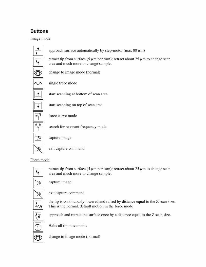
ButtonsImage mode

approach surface automatically by step-motor (max 80 µm)

retract tip from surface (5 µm per turn); retract about 25 µm to change scanarea and much more to change sample.

change to image mode (normal)

single trace mode

start scanning at bottom of scan area

start scanning on top of scan area

force curve mode

search for resonant frequency mode

capture image

exit capture command

Force mode

retract tip from surface (5 µm per turn); retract about 25 µm to change scanarea and much more to change sample.

capture image

exit capture command

the tip is continuously lowered and raised by distance equal to the Z scan size.This is the normal, default motion in the force mode

approach and retract the surface once by a distance equal to the Z scan size.

Halts all tip movements

change to image mode (normal)

!

parameters for image modeScan controls:

scan size: Size of the scan along one side of the square. If the scan is non-square (asdetermined by the aspect ratio parameter), the value entered is the longer of the twosides. Maximum/minimum value: 500 nm - 10 µm.

aspect ratio: determines whether the scan is to be square (aspect ratio 1:1), of non-square. Default value 1:1.

X offset, Y offset: these controls allow adjustment of the lateral scanned area and thecenter of the scanned area. These values can be chosen between 0 and maximal 10µm, depending on the scan size (piezo deflection in x- and y-direction is max. 10µm).

scan angle: combines X-axis and Y-axis drive voltages, causing the piezo to scan thesample at varying X-Y angles. Value between 0 and 90 degrees.

scan rate: the number of lines scanned per second in the fast scan (X-axis on displaymonitor) direction. In general, the scan rate must be decreased as the scan size isdecreased. Scan rates if 1.5-2.5 Hz should be used for larger scans on samples withtall features. High scan rates help to reduce drift, but they can only be used on veryflat samples with small scan sizes. Maximum/minimum value: 0.1 Hz - 5 Hz.

tip velocity: the scanned distance per second in the fast scan direction (changes as thescan rate changes).

samples/line: number of imaged points per scanned line. Maximum/minimum value: 128- 1024 (default value 512).

lines: number of scanned lines. This value is the same as samples/line for aspect ratio of1:1. Maximum/minimum value: 128 – 1024; default value 512.

number of samples: sets the number of pixels displayed per line and the number of linesper scanned frame.

slow scan axis: starts and stops the slow scan (Y-axis on display monitor). This control isused to allow the user to check for lateral mechanical drift in the microscope or assistin tuning the feedback gains. Always set to ‘enable’ unless checking for drift ortuning gains. Default value: enable

Feedback controls:

SPM feedback: sets the signal used as feedback input. Possible signals are ‘Amplitude’(default), ‘TM deflection’ and ‘Phase’.

integral gain and proportional gain: controls the response time of the feedback loop.The feedback loop tries to keep the output of the SPM equal to the setpoint referencechosen. It does this by moving the piezo in Z to keep the SPM’s output on track withthe setpoint reference. Piezoelectric transducers have a characteristic response time tothe feedback voltage applied. The gains are simply values that magnify the differenceread at the A/D converter. This causes the computer to think that the SPM output isfurther away from the setpoint reference than it really is. The computer essentiallyovercompensates for this by sending a larger voltage to the Z piezo than it trulyneeded. This causes the piezo scanner to move faster in Z. This is done to compensate

for the mechanical hysteresis of the piezo element. The effect is smoothed out due tothe fact that the piezo is adjusted up to four times the rate of the display rate.Optimize the ‘integral gain’ and ‘proportional gain’ so that the height image showsthe sharpest contrast and there are minimal variations in the amplitude image (theerror signal). It may be helpful to optimize the ‘scan rate’ to get the sharpest image.Maximum/minimum value for integral gain: 0.1 – 4 and for proportional gain: 0.1 –10. Default values between 2 and 3.

amplitude setpoint: The setpoint defines the desired voltage for the feedback loop. Thesetpoint voltage is constantly compared to the present RMS amplitude voltage tocalculate the desired change in the piezo position. When the SPM feedback is set toamplitude, the Z piezo position changes to keep the amplitude voltage close to thesetpoint; therefore, the vibration amplitude remains nearly constant. Changing thesetpoint alters the response of the cantilever vibration and changes the amount offorce applied to the sample. Maximum/minimum value: 1 – 8.

drive frequency: defines the frequency at which the cantilever is oscillated. Thisfrequency should be very close to the resonant frequency of the cantilever. Thesevalue is around 300 kHz for the cantilevers used.

drive amplitude: defines the amplitude of the voltage applied to the piezo system thatdrives the cantilever vibration. It is possible to fracture the cantilever by using toohigh drive amplitude; therefore, it is safer to start with a small value and increase thevalue incrementally. If the amplitude calibration plot consist of a flat line all the wayacross, changing the value of this parameter should shift the level of the curve. If itdoes not, the tip is probably fully extended into the surface and the tip should bewithdrawn before proceeding. Maximum/minimum value: 10 – 60, default 30 V.

Channel 1, 2 and 3

data type: height data corresponds to the change in piezo height needed to keep thevibrational amplitude of the cantilever constant. Amplitude data describes the changein the amplitude directly. Deflection data comes from the differential signal off of thetop and bottom photodiode segments.

data scale: This parameter controls the vertical scale corresponding to the full height ofthe display and colorbar.

data center: Offsets centerline on the color scale by the amount entered.line direction: Selects the direction of the fast scan during data collection. Only one-way

scanning is possible.Range of settings:• Trace: Data is collected when the relative motion of the tip is left to right as

viewed from the front of the microscope.• Retrace: Data is collected when the relative tip motion is right to left as viewed

from the front of the microscope.scan line: The scan line controls whether data from the Main of Interleave scan line is

displayed and captured.realtime plane fit: Applies a software ‘leveling plane’ to each real-time image, thus

removing up to first-order tilt. Five types of planefit are available to each real-timeimage shown on the display monitor.

Range of settings:• None: only raw, unprocessed data is displayed.• Offset: takes the Z-axis average of each scan line, then subtracts it from every data

point.• Line: takes the slope and Z-axis average of each scan line and subtracts it from

each data point in that scan line. This is the default mode of operation, and shouldbe used unless there is a specific reason to do otherwise.

• AC: takes the slope and Z-axis average of each scan line across one-half of thatline, then subtracts it from each data point in that scan line.

• Frame: level the real-time image based on a best-fit plane calculated from the mostrecent real-time frame performed with the same frame direction (up or down).

• Captured: level the real-time image based on a best fit plane calculated from aplane captured with the capture plane command in.

off line plane fit: Applies a software ‘leveling plane’ to each off-line image for removingfirst-order tilt. Five types of plane-fit are available to each off-line image.Range of settings:• None: only raw, unprocessed data is displayed.• Offset: captured images have a DC Z offset removed from them, but they are not

fitted to a plane.• Full: A best-fit plane that is derived from the data file is subtracted from the

captured image.highpass filter: This filter parameter invokes a digital, two-pole, highpass filter that

removes low frequency effects, such as ripples caused by tortional forces on thecantilever when the scan reverses direction. It operates on the digital data streamregardless of scan direction. This parameter can be ‘off’ or set from 0 through 9.Settings of 1 through 9, successively, lower the cut-off frequency of the filter appliedto the data stream. It is important to realize that in removing low frequencyinformation from the image, the highpass filter distorts the height information in theimage.

lowpass filter: This filter invokes a digital, one-pole, lowpass filter to remove high-frequency noise from the Real Time data. The filter operates on the collected digitaldata regardless of the scan direction. Settings for this item range from ‘off’ through‘9’. Off implies no lowpass filtering of the data, while settings of 1 through 9,successively, lower the cut-off frequency of the filter applied to the data stream.

parameters for force modeMain control

ramp channel: Defines the variable to be plotted along the X-axis of the scope trace.Default ‘Z’.

ramp size: This parameter defines the total travel distance of the piezo. Use cautionwhen working in the force mode. This mode can potentially damage the tip and/orsurface by too high values for the ramp size.

z scan start: This parameter sets the offset of the piezo travel (i.e., its starting point). Itsets the maximum voltage applied to the Z electrodes of the piezo during the forceplot operation. The triangular waveform is offset up and down in relation to the valueof this parameter. Increasing the value of the ‘z scan start’ parameter moves thesample closer to the tip by extending the piezo tube.

scan rate: sets the rate with which the Z-piezo approach/retract the tip.Maximum/minimum value: 0.1 Hz - 5 Hz.

X offset and Y offset: controls the center position of the scan in the X- and Y- directions,respectively; same as in image mode. Range of settings: ±220 V.

number of samples: Defines the number of data points captured during eachextension/retraction cycle of the Z-piezo. Maximum/minimum value: 128-1024;default value 512.

average count: sets the number of scans taken to average the display of the force plot.May be set between 1 and 1024. Usually it is set to 1 unless the user needs to reducenoise.

spring constant: This parameter relates the cantilever deflection signal to the Z travel ofthe piezo. It equals the slope of the deflection versus Z when the tip is in contact withthe sample. For a proper force curve, the line has a negative slope with typical valuesof 10-50 mV/nm; however, 10-50 mV/nm; however, by convention, values are shownas positive in the menu.

display mode: The portion of a tip’s vertical motion to be plotted on the force graph.Range of settings:• Extend: plots only the extension portion of the tip’s vertical travel.• Retract: plots only the retraction portion of the tip’s vertical travel.• Both: plots both the extension and retraction portion of the tip’s vertical travel

units: this item selects the units of the parameters, either ‘metric’ lengths or ‘volts’.X-rotate: allows the user to move the tip laterally, in the X direction, during indentation.

This is useful since the cantilever is at an angle relative to the surface. One purpose ofX rotate is to prevent the cantilever from plowing the surface laterally, typically alongthe X direction, while it indents in the sample surface in the Z direction. Plowing canoccur due to cantilever bending during indentation of due to X movement caused bycoupling of the Z and X axes of the piezo scanner. When indenting in the Z direction,the X rotate parameter allows the user to add movement in the X direction. X rotatecauses movement of the scanner opposite to the direction in which the cantileverpoints. Without X rotate control. The tip may be prone to pitch forward duringindentation. It can be varied in a range of 0-90 degrees. Normally, it is set to about 22degrees.

amplitude setpoint: same as in image mode.Channel 1, 2 and 3

data type/data scale/data center: same as in image mode.amplitude sens.: This item relates the vibrational amplitude of the cantilever to the Z

travel of the piezo. It is calculated by measuring the slope of the RMS amplitudeversus the Z voltage when the tip is in contact with the sample. The NanoScopesystem automatically calculates and enters the value from the graph after the operatoruses the mouse to fit a line to the graph. This item must be properly calculated andentered before reliable deflection data in nanometers can be displayed. For a properforce curve, the line has a negative slope with typical values of 10-50 mV/nm;however, 10-50 mV/nm; however, by convention, values are shown as positive in themenu.

Trouble shootingIt happens rather often that one thinks to have checked all control panel parameterscorrectly and don’t get an image. Here a list with the most common errors.• Right input channel (see monitor). ‘Height’ signal for constant height and ‘deflection’

signal for constant deflection mode.• Correct gains for ‘proportional gain’ and ‘integral gain’. These parameters have to be

between 0.1 and 5, depending on the softness/hardness of the sample. Start with the‘integral gain’ set to 0.50 and the ‘proportional gain’ set to about 1.20.

• Is the height scale justified correctly for the different channels.• What is the size of the scan area. The scan size can be varied between 100 nm and 10

µm. Use a scan size of 10 µm to get an overview.• Is the piezo in its limit; between + of – 220V. This can be checked by the green/red

setpoint line in the approach/retract bar. This green/red setpoint line should not be onthe left or on the right site of the bar. This can be changed by the ‘amplitude setpoint’parameter.

• Does the force used to image the probe, destroy the probe. Play around with the‘amplitude setpoint’ parameter and the ‘drive amplitude’ parameter. The slope of theforce curve shows the sensitivity of the TappingMode measurement. In general,higher sensitivities will give better image quality. The View -> Force Mode -> plotcommand plots the cantilever amplitude versus the scanner position (=force curve).The curve should show a mostly flat region where the cantilever has not yet reachedthe surface and the sloped region where the amplitude is being reduced by the tappinginteraction. To protect the tip and sample, take care that the cantilever amplitude isnever reduced to zero. Adjust the setpoint until the green setpoint line on the graph isjust barely below the flat region of the force curve. This is the setpoint that applies thelowest force on the sample.

Poor image qualityContaminated tip

Some types of samples may adhere to the cantilever and tip (e.g. certain proteins). Thiswill reduce resolution giving fuzzy images. If the tip contamination is suspected to be aproblem, it will be necessary to protect the tip against contamination.Dull tip

AFM cantilever tips can become dull during use and some unused tips may be defective.If imaging resolution is poor, try changing to a new cantilever.Multiple tip

AFM cantilevers can have multiple protrusions at the apex of the tip which result inimage artifacts. In this case, features on the surface will appear two or more times in theimage, usually separated by several nanometers (see figure 2A). If this occurs and thiseffect doesn’t disappear after some time, change of clean the AFM tip.

Repeating pattern

If a repeating pattern appears, more tip areas scan simultaneous (see figure 2B). Such acantilever has to be changed.To low setpoint

Some structure shows up that don’t exist (e.g. circles). Change the ‘amplitude setpoint’ toa better value.To high setpoint

If silverfish structures appear (see figure 2C), the adjustment of the integral andproportional gain can help, but if the setpoint is not adjusted correctly, increasing the gainwill worse the noise of the image.To high Drive frequency

The image surface looks destroyed; e.g. holes appear. These holes are artifacts anddisappear when the drive frequency is lowered.Other error sources

• Scanner beeps loud: decrease immediately the gains; the scanner is overdriven.• The image seems only noise: Adjust ‘amplitude setpoint’.• Strong drift of signal: approach the tip from the surface with the 2nd button in the

upper screen and retract again.• During retraction of the tip, the scanner shows immediately contact with the surface,

the image shows only noise: check the setpoint. Put the setpoint to zero and approachthe surface again.

Figure 2 (A) multiple tip, (B) repeating patterns and (C) Silverfish structures due tohigh setpoint.

TheorieSurface Measurement ParametersFrom the measured surface images, it is possible to make an estimation of the smoothnessof the surface. With the following image processing equations, one can quantify surfacesmathematical.

Term Definition Calculation UseZ Mean Value

€

Z =1N

Zii=1

N

∑where N is the number of datapoints, and Z is the surface height

Ra Roughness average is themain height as calculatedover the entire measuredlength or area. It is quotedin micrometers.

Two-dimensional Ra:

€

Ra =1N

Zi − Zi=1

N

∑Three-dimensional Ra:

€

Ra =1MN

Zij − Zi=1

M

∑j=1

N

∑where M and N are the number ofdata points in X and Y, and Z is thesurface height relative to the meanplane.

Ra is typically used todescribe the roughness ofmachined surfaces. It isuseful for detecting generalvariations in overall profileheight characteristics and formonitoring an establishedmanufacturing process.

RRMS The Root Mean Square(RMS) average betweenthe height deviations andthe mean line/surface,taken over the evaluationlength/area.

Two-dimensional RRMS:

€

RRMS =1N

Zi − Z( )2

i=1

N

∑Three-dimensional RRMS:

€

RRMS =1NM

Zij − Z( )2

i=1

N

∑j=1

M

∑

RMS roughness describesthe finish of optical surfaces.It represents the standarddeviations of the profileheights.

Z

Z

RtRv

Rp

RRMS

Figure 1. a schematic image of an image profile

Table I: surface measurement parameters

Rp, Rv Maximum profile peakheight and maximumprofile valley depth are thedistances from the meanline/surface to thehighest/lowest point in theevaluation length/area.

Measured Peak height providesinformation about frictionand wears on a part. Valleydepth provides informationabout how a part mightretain a lubricant.

Rt Maximum height is thevertical distance betweenthe highest and lowestpoints in the evaluationlength/area.

€

Rt = Rp + Rv Maximum height describesthe overall roughness of asurface.

Rz The average maximumprofile of the ten greatestpeak-to-valley separationsin the evaluation area.Vision excludes an 11 × 11region around each high(H) or low (L) point suchthat all peak or valleypoints won’t emanate fromone spike or hole.

€

Rz =110

Hii=1

10

∑ − L jj=1

10

∑

Rz is useful for evaluatingsurfaces texture on limited-access surfaces such assmall valve seats and thefloors and walls of grooves,particulary where thepresence of high peaks ordeep valleys is of functionalsignificance.

Preparation tasksWhat are the limits of the resolution of an optical microscope, according to Abbe’sequation. See also: http://www.uiowa.edu/~cemrf/courses/light/light.htm. What limits theresolution of an Atomic Force Microscope.

What are piezo-materials and how can one use these in motion systems. See also:http://www.piezo.com/bendedu.html

Describe how a closed-loop (feed-back) control functionize. Discuss what happens withthe measured image by changing the values for P and I (proportional and integrationgain). See also:http://www.netrino.com/Publications/Glossary/PID.htmlhttp://www.engin.umich.edu/group/ctm/PID/PID.html#characteristics

Calculate the values for mean, Ra and RRMS, for a line profile of a cosine-function with 5periods within the measure length and for a cosine-function with 5.25 periods with in. Dothis for a line profile with 200 points and for a line profile with 50 points.

ExperimentsGoal of these experiments is to learn about the basic functioning and possibilities of theAtomic Force Microscope. The structure of a few surfaces will be observed andquantified. Also some biological samples will be imaged and researched.

Material• AFM-cantilevers• Calibration grid• Metal plate• Glass plate• Mica plate• Superglue• Pair of tweezers• Tesa-film• Biological probes (ask for)

Introductory experimentsP and I values

1. Vary the values of the proportional gain P and the integral gain I, while imagingthe surface of a calibration grid. Try to find optimal values for both parameters.Discuss the effect of high/low proportional and integral gain with respect to theimage quality versus a reliable height measurement. (see webpages under‘preparation tasks’ for a theoretical explanation of PD-controller)

Tip characterization

1. Make an image of a calibration grid to characterize the size of the AFM tip. Thecalibration grid has a rectangular shape in XY direction. The tickness of the gridwall is about 100 nm in average build on the surface with a triangular shape in XZdirection (see figure below). Calculate the AFM tip-radius using the recordedAFM image of the calibration grid.

1 µm 100 nmX

YZ

Surface quantification

1. Make two AFM-images of a glass surface; one with a scan size of 500 nm andone with a scan size of 10 µm.

2. The same as point 1, but now with a mica-surface.3. Use the surface parameters shown in table I to quantify the surfaces imaged under

1 and 2 for both the 500 nm and the 10 µm image. Describe and discuss theresults. (height DNA is about 2 nm).

Force-Distance Curve

1. Use a mica-surface to make an approach and retract force-distance curve. Discussthe different parts of the curve as e.g. approach of the surface, position of thesurface, peaks etc..

Amplitude/Phase imaging

1. Make an AFM image of the sticky side of a tesa-film. This imaging shouldinclude a height image, a phase image and an amplitude image.

2. Describe the differences between these three images (theoretical) and discuss therecorded data with respect to information output.

Biological probesChromatin fiber

Make an image of a chromatin fiber (scan size about 1 µm). Chromatin is a DNA fibercompacted by nucleosomes; the DNA is wrapped about 2 times around this protein (seefigure below). Determine the size of a nucleosome (radius, height) and estimate thelength of the DNA compacted in the recorded chromatin fiber. Discuss these measuredsizes.

Human Hair

Make an image of a human hair and determine the height of the steps on it. The period ofthese steps are about 4 µm.

Cell wand

Make an image of the outside of a cell wand. Make also a force-distance curve on the cellwand and discuss the differences with the one recorded above on mica.Chromosomes

Search for chromosomes with the optical microscope and make an AFM image of one.Show the height profile of one ‘leg’ of this recorded chromosome.

Own materials

Imaging of your own interesting materials. E.g. paper