atomic timekeeping and the statistics of precision … august 1960. ire, voi. 48, pp, 1167-1473,...

PROCEEDINGS OF THE IEEE VOL. 54, NO. 2 FEBRUARY, 1966

ACKNOWLEDG~I ESI

\;C‘e would like to thank Dr. R. F. Lace?. for his assistance in the course of this .v\-ork. M’e are indebted to L. S. Cutler of the Henlett-Packard Cornpan),, Palo Alto, Calif., and Prof. C. I,. Searle of the llassachusetts Institute of Technology, Cambridge, for many in- formative and constructive discussions.

RE FEKENC 1.: S

Cutler aiid C. L. Searle, “Some aspects of the theory and urement of frequency fluctuatioiis in frequency standards,”

this issue, page 136. 121 I). \!. Allan, “The statistics of atomic frequent), standards,”

this issue, page 221. [ 3 ] 31. E. Packard and 12. C. R y p e l , “The rubidium optically

pumped frequency standard, N E R E M Record, Sovember 1961.

[4] I<. I;. C. Vessot, “Frequency stability measurements between several atomic hydrogen masers,” in Quantun? Electronics I I I . New York: Columbia L’niversity Press, 1961.

[SI 1:. Van Duzer, “Short-term stability measurements,” Pvoc. I964 IEEE-N.4 SA Symp. on the Definition and Jifeasz4rentenl of Short- Term Frequency Stability. \Vashington, D. C.: [-, S. Govt. Print- ing Office, NAS.4 SP-80, 1965, pp. 269-272.

(61 J. Vanier and 12. F. C. Vessot, “Cavity tuniiig aiid pressure dependence of frequency in the hydrogen maser,” dppl. Phys . Letters, vol. 4, p. 122-123, April 1964.

(71 L. S. Cutler, “Some aspects of the theory and measurement of frequency fluctuations in frequency standards,” op. cit. [5], pp.

[8] C. L. Searle e t al., “Computer-aided calculatioii of frequency stability,” op. (it. 151, pp. 273-277.

[9] E. J . Raghdady, K. I) . Lincoln, and B. TI. Seliii, “Short-term frequency stability: characterization, theory and ineasurement,” op. c i t . 151, pp. 65-87.

[IO] J . .A. Barnes and D. I\.. .Wen, “Effects of long-term stability on the delinition and nieasiiremeiit of short-tern1 stability,” o p . cit.

[I 11 J . A. Barnes, “Xtomic timekeeping and the statistics of precision signal generators,” this issue, page 207.

1121 \V. A. Edson, “Soise in oscillators,” Proc. I R E , vol. 48, pp.

[13] M , J . E. Golay, “Monochromaticity and noise in a regenerative electrical oscillator,” Proc. I R E , v-01. 48, pp. 1473-1477, August 1960.

[14] J . A. hlullen, “Background noise i i i nonlinear oscillators,” Proc.

1151 K. Shimoda, T. C. \\‘ang, and C. 11. ‘l‘ownes, “Further aspects of the theory of the maser,” Phys. Reo., vol. 102, p. 1308-1321, June 1956.

[I61 D. Kleppiier, H. 11. Goldenberg, and N . F. ICamsey, “Theory a t the h>,drogen maser,’‘ Z’hys. Ret’., vol. 126, p. 603-615, April 1962.

[17] J . Vanier, H . E. Peters, and I<. I:. C. Vessot, “Exchange colli- sions, wall interactions, and resettability of the hydrogen maser,” I E E E Trans. on Instrimenlalion and Xeasurement, vol. 1M-13, pp. 185-188, December 1964.

[l8] .I. McFoubrey, “A survey of atomic time and frequency standards, this issue, page 116.

89-100.

[SI, pp. 119-123.

1454-1456, August 1960.

I R E , VOI. 48, pp, 1167-1473, AugtIst 1960.

Atomic Timekeeping and the Statistics of Precision Signal Generators

JAMES A. BARNES

Abstract-Since most systems that generate atomic time employ quartz crystal oscillators to improve reliability, it is essential to determine the effect on the precision of time measurements that these oscillators introduce. A detailed analysis of the calibration procedure shows that the third finite difference of the phase is closely related to the clock errors. It was also found, in agreement with others, that quartz crystal oscillators exhibit a “flicker” or / W -I type of noise modulating the frequency of the oscillator.

The method of finite differences of the phase is shown to be a powerful means of classifying the statistical fluctuations of the phase and frequency for signal generators in general. By employing finite differences it is possible to avoid divergences normally associated with flicker noise spectra. Analysis of several cesium beam frequency standards have shown a complete lack of the 1 W I --I type of noise modulation.

INTKODI-CTION

N ORDISARJ7 clock consists of tn-o basic systems: a periodic phenomenon (pendulum), and a counter (gears, clock face, etc.) to count the

Manuscript received September 8, 1965 ; revised November 6,

The author is with the National Bureau of Standards, Boulder, 1965.

Colo.

periodic events. .An atomic clock differs fro11’ this only in that the frequenq. of the periodic phenomenon is, in some sense, controlled by an atoniic transition (atomic frequent), standard). Since microwave spectroscopic techniques allo\\- frequencies to be measured \vith a relative precision far better than any other quantity, the desirabilit). of extending this precision to the domain of time nieasurenient has long been recognized [l].

From the standpoint of precision, i t would be desirable to run the clock (counter) directly from the atomic frequent! standard. How ever, atomic frequency standards in general are sufficient11 complex that reliable operation over very extended periods becomes some- what doubtful (to say nothing of the cost involved). For this reason, a quartz crystal oscillator is often used as the source of the “periodic” events to run a synchro- nous clock (or its electronic equivalent). The frequency of this oscillator is then regularly checked by the atomic frequency standard and corrections are made.

These corrections can usually take on any of three forms: 1) correction of the oscillator frequency, 2 ) correction of the indicated time, or 3) an accumulating

207

208 PROCEEDINGS OF THE IEEE FEBRUARY

I I I I I I I

record of the difference from ,itomic time of the apparent or indicated time sho\\n by the clock. Both methods 1) and 2 ) require a calculation of the time difference, and it is sufficient to consider 0111) the last method and the errors inherent in it.

careful consideration of the calibration procedure leads to the development of certain functionals of the phase which have a very important property-existence of the variance even in the presence of a flicker (1 ' 1 w ( 1 type of frequencq noise. The simplest of these functionals, the second and third finite differences of the phase, turn out to be stationary, random variables \\.hose auto-covariance function is sufficientl?. peaked to insure rapid convergence of the variance of a finite sample toward the true (infinite sample) variance. These functionals of the phase have the added features of being closely related to the errors of a clock run froin the oscillator as well as being a useful nieasure of oscillator stabilit!..

Vf'ith the aid of these functionals, it is possible to classify the statistical fluctuations observed in various signal sources. In agreement with uork of others [2]-[5], a flicker noise frequency inodul,ition \vas oh- served for all qunrtz cr? stal oscillators tested. Similar studies on several commercial rubidium gas cells g'ive uniform indications of flicker noise modulation of levels comparable to those of the better quartz cr\rstal oscillators.

In Section I , the effects on the precision of a time scale due entirely to the calibration procedure of the quartz crystal oscillator and the oscillator's inherent frequent), instability are considered.

I n Section 11, the experimental results of Section I are used as the basis for a theoretical model of oscillator

I I I I

IS1

121

df I

0 x - + '1

:: 8

w

e e 2 k

- 4 c

W

- I C

-12c

-IS(

frequency fluctuations, and the results are compared to those of other experimenters.

In Section 111, the statistics of <in atomic frequent) standard of the passive type (e.g., Cs-beam or Iib-gas cell) are considered, and the composite Clock system is treated. Section I\' is devoted to a brief discussion of stability measures for signal sources.

I . Q r - a K n CKTSTAL OscII.I..\n)K €'fr:\si; I ~ r , ~ ~ ( ~ , ~ ~ ~ . ~ , i ~ r o ~ s

Typical Gross Belzaaior Figure 1 shon-s a t!.pical aging curve for ;L fairlJ- good

quartz cr)-stal oscillator. The oscillator had heen operating for a fe\v months prior to the date shoivn i n the graph. On 3Ta~- 1 , 1963, the frequency of the oscillator \ \as reset in order to maintain relatively small corrections.

Least square fits of straight lines to the tn-o parts of Fig. 1 yield aging rates of 0.S36X10-10 per day and 0.515 X 10-l0 per da)., respectivelJ-. This difference i n aging rates could be explained by a n acceleration of the frequency of about -9X10-'5 per da>- per day. This acceleration of the frequency is suflicientl\~ small over periods of a feu- da>.s \\-hen compared to other sources of error tha t i t can be safely ignored. Thus, the frequency of conventional quartz oscillators cau be i\.rit ten in the form

Q ( t ) = nap + at + € ( t ) ] (1)

\\.here a is the aging rate, ;(t) is a variation of the frequenq- probably caused by noise processes i n the oscillator itself, and t can he considered to be sotlie rather gross nieasure of the time (since a and i are quite small corrections).

I I I I I I I I I I I I 1 1 - 1 - 1

1966 BARNES: ATOMIC TIMEKEEPING AND PRECISION SIGNAL GENERATORS 209

.4ctual Calibration Procedure of a Clock System

is 163 The fundamental equation for atomic timekeeping

where Q is the instantaneous frequency of the oscillator as measured by an atomic frequency standard, dcp is the differential phase change, and d t is an increment of time as generated by this clock system. Since time is to be generated by this system, and 4 and $1 are the directly measured quantities, i t is of convenience to assume that Q=Q(+) and to write the solution of (2) in the form,

If one divides the output phase of the oscillator by f&, and defines the apparent or indicated time t A to be

4 QO

t A = - >

(1), ( 3 ) , and (4) can be combined to give

4 s it is indicated in Fig. 1, it is possible to maintain the magnitude of the relative frequency offset 1 LvtA +;I within fixed bounds of lop8. Expanding ( 5 ) to first order in this relative frequency offset yields

Equation (6) should then be valid to about one part in lo'6.

Normally the frequency of the oscillator is measured over some period of time (usually a few minutes) a t regular intervals (usually a few days). At this paint, i t is desirable to restrict the discussion to the case where the calibration is periodic (i.e., period T, determined by t A ) and then generalize to other situations later. One period of the calibration is as follows:

t A start of calibration interval tA+&(T-7 ) star t of frequency measurement ( r < T ) t A +&(T+T) end of frequency measurement

t A +I" end of calibration interval,

At = Af.4 - TI- 6f2 \ \ 52" L' ( 7 )

where (6fl/Qo), is the average relative frequency offset during the interval t A + + ( 2 ' - ~ ) to tA++(T+7).

Even though, in general, i is not constant, E and i are not knowable, and thus one is usually reduced to using (7) anyuay . The problem, then, is to determine how much error is introduced by using ( 7 ) .

The time error 6t accumulated over an interval '1' conimitted by using ( 7 ) can be expressed in the form,

where the quantity {6Q/flo)7 is given by

Equations (8) and (9) can be combined to give

- '[.(t4 7 + y) - +3]. (10)

I t is this equation which relates the random phase fluctuations with the corresponding errors in the time determination.

M e a n i n g f u l Quanti t ies

I t is again of value to further restrict the discussion to a particular situation and generalize a t a later point. In particular, let I'= 37, then (10) beconies

6t = € ( t A + 3r) - € ( L A ) - 3[&4 + 27) - € ( t A + 7)]. (11)

I t is now possible to define the discrete variable b). the relation

E n E €([A + H T ) , ?E = 0, 1, 2, ' ' '

and rewrite (11) in the simpler forni (see Table I )

6t E A%,,, (12)

where A3e, is the third finite difference of the discrete variable E , ~ .

where T is the frequency measurement interval. If i were constant in time, the frequency measured during the interval t A $ $ ( T - 7 ) to t.1+$(T+r) would be just the average frequency during the complete measurement interval T since the oscillator would have an exactly linear drift in frequency. Also, i f i were con- s tant , (6) could be written as

210 PROCEEDINGS OF THE IEEE FE BRUAKY

Similarly, ( 2 ) mal. be integrated directl), using (1) to If three oscillators are used, i t is possible to indepen- dently measure the three quantities u1z, crI3, and (T23. Thus obtain there exist three independent equations :

1 (TI22 = (TI2 + u.92 cy + 4.4 + d o ) . (13)

Thus, by defining another discrete variable +,,, the third difference of (13) yields t h e relation

A’+, = bloA3en, (l’) While the three equations,

i, j = 1 , 2 , 3 or equivalently,

j i < j

are not linearli independent, the standard deviations u,]? given b) (1X) , in fact, foriii l inexl j independent equations (su b j ec t on 1 y to cer ta 1 n con d i ti on s m,il ogo u s

Si,, A3en(’) - A3e,,(3) 1

61 = (13

I t is non possible to set up ‘1 t,ible of meaningful quantities for time measurement (see Table I I )

I;irst difference of the phase ]A#,, 1 Proportioiial to the average freqiienc). i n the interval r . Must exist for :!I1 time.

Second ditfereiice of the ph,i\e ]Az@,, 1 Related to the drift of the oscillator frequency Must exist for ‘ill time

Variance of the second dilfereiice\([.!,%$,,- (1Z#,J]’2) (It is possible to construct a time scale even if this does riot exist. How-ever, experimeiit I indicates that it is probably finite.)

Third difference of the phase IA34,, Proportion;il to the clock error i n the time interval T = 3 r . LIust exist if clock is to be of value.

\Iean q u x e third tliltereuce j ( (A3@,,) )? I Proportiorial to the precision of time wterv,il measureinent~. \lust exist if clock 15 t o he 1 of value - ~- ~~ - -

U here all ,iverageb are delined b> the relation:

IXxperLmenfal Determinat ion of Phase Fluctuations If one mecisiires the phase difference bet\\-een t \ \o

oscillators, (15) applies t o both, and hence the difference phase 8,, =&(ll -+,,(?) is related to the difference time 6 f i z = 6 t l - 6 t 2 by the relations

1

RO B t 1 2 = --- A30,, = A3e,, L, - A 3 ~ , , ( r ) . (16)

Provided that the cross-correlation coefficient ((43t,,(11)

(A3cn(?)) ) is zero (i e., the l ’ are noncorrelated), the variance of 6 t l s becomes

u,s? E ((S!]?)?) = ( (A3€, , ( ’ ’ )?) + ( ( A 3 € n ( 1 ’ ) 2 ) , (17)

since it is assunied th,tt (A3e,,) = 0. The assumption that the cross-correlation coeflicients vanish is equivalent to postulating an absence of linear coupling betu een the oscillators either electricall> or through their environ- ment. I t is of value to develop a scheme lvhich is capa- ble of classifying individual oscillators rather than treating ensenibles of assumed identical members. Thus, this development is restricted to time averages of individual oscillators rather than ensemble averages.

to the triangle inequalities). Thus, the systems of (18) are solvable for the three quantities u L 2 = ( ( 6 t J 2 ) . I t is thus possible to estimate the statistical behavior of each individual oscillator.

A pparatus A phase meter n-as used similar to one described in

Cutler and Searle [SI. The basic sq,steni was aligned Ivith an electrical-to-mechanical angle tolerance of about kO.25 percent of one complete cycle, and since the phase meter is operated a t 10 I ~ T c ~ s , this implies the possibility- of measuring the time difference to f 0.25 nanoseconds. The output shaft, in turn, drives a digital encoder with one hundred counts per revolution and a total accumulation (before starting over) of one million. Thus the digital information is accurate to \\-ithin one ns and accumulates up to one tiis. Since ineasurements are made relatively often, it is easy for a computer to spot \\-hen the digital encoder has passed one ins on the data , and this restriction on the data format in no \vay hampers the total length of the data handled.

Since the oscillator is assumed to have ;I linear drift in frequenci, \vith time, the variance (about the mean)

1966 BARNES: ATOMIC 'TIMEKEEPING AND PRECISION SIGN.41- GENER,%TORS 211

of the second difference of the phase should depend onlj on the e n ( & ) l:or the evaluation of clocks, it is the mean squ,ire time error u hich is important and, thus, the nie<in square (r'ither th'tn vxiance) of the third difference of the ph'ise is the cjunntitj of iniportance. Calcu- Intions of these qumti t ies froni the phase d,, \I ere x - coniplished on a digit,il coniputer Yormnll\ the phase difference is printed e%er\ hour for a t least 200 hours m d the computer progr,im coniputes the AW,, and add,, for eclu'il t o 2 , 4, 6, 8, etc , hours. Thus it is possible to plot the square root of the varimce of the second differerice and the root nienn square third difference of t h e ph.ise <IS <I function of the vxiab le T ;i t j pica1 plot of these t n o quantities appears in Fig. 2.

300

I / I DAY 2 DAYS I

I I I I I l l l l I I 20 30 40 50 60 80 100 200

IO IO

TIME ( KILOSECONDSI

Fig. 2. Variance of second a i d third difference as a function of 7 .

Since n i a n ~ ~ revolutions of the phase meter are normally encountered betiyeen data points, the combined effects of nonperfect electrical-to-mechanical phase and rounding errors of the digital encoder can be combined into one stationary, statistical quantity y, tha t can be assumed to have delta-function auto-correlation. Let x represent the rounding errors of the digital encoder defined by the difference betiyeen the encoded number and the actual angular position of the shaft. Then these rounding errors form a rectangular distribution from -0.5 ns to fO.5 ns, and, t h u s , contribute an amount

x' dx = 0.08 ns:

l i 2

dx

to ( y 2 ) . The nonperfect electric,il-to-inechanical phase conversion is sinusoid,il in n ~ t u r e 'ind, thus, contributes an miount equal to

4(0.25)? = 0.03 ns?

The final value for (y?) should then be 'tbout 0.11 lis?

'I'his \ \as checked b j t,tking trio ver) good oscillators operating a t a rather large difference frequent), (-5 X and printing the ph.Lse difference ever) 10 seconds for several minutes Since frequencj fluctu'itions of the oscilhtors are small compared to 1 X 10-ln, the resultant scntter cdn be 'ittributed to the nieasuring s\ s- tem. The results of this experiment gave the value 0.19 ns2 for (y?).

Since y is assumed to have 'i delta-function auto-correlation, reference to Table I shou s tha t ( (A3y)2) =20(y2j, and thus (18) may be more precisel? nr i t ten,

(18') 1 u12' = cT12 + cT22 + 20(y9

cT13 = UI2 + (73' + 20(y2) . c 2 3 = 'S22 + cX2 + 20")'') 1

For the best oscillators tested, crt,2 became about 2((A3y)2j for T = l o 3 seconds, and, therefore, measurements nere limited on the louer end to 20 minutes or 1200 seconds. The longest run ninde lasted a little over '1 month or about one thousand hours. Thus the largest value of T \\ hich might have reason'ible avernging is ,ibout one hundred hours or 3.6X lo5 seconds. This lini- its the results to about t n o orders of magnitude variation on r.

\I-hile i t is possible to build appropriate frequenc) multipliers and mixers to improve the resolution of the phase meter and reduce the lower limit on T , it \\as considered thnt the longer time intervals are of greater interest because T (= 3 ~ ) is norni,illy bet\\ een one da) m d one week.

I I . THEORETICAL DISVELOPMEN I'

Introdiictory Remarks In the development \I hich follou s, certain basic as-

sumptions are made I t is assuined that the coefficients 9, and a of (1) ma) be so chosen tha t the average value of ~ ( t ) is zero; i.e.,

( e ( / ) ) = 0.

I t is also .issunled tha t '1 translation in the time axis, t4-+t4 +{, (stationarity) cnuses no change in the value of the auto-covariance function,

R,(7) = ( € ( t ) . € ( t + 7)) = ( € ( t + t ) . €0 + E + 7)). (19)

The only justification of this assumption lies in the fact that the results of the m a l j sis agree \I ell u-ith experiment and the results of others. In the development n hich follows, one caiznot assume tha t

RAO) = ([4012)

2 12 PROCEEDINGS OF THE IEEE FEBRUARY

exists (i.e., is finite) and, hence, Ll’iener [ 7 ] cannot guarantee that (19) is valid. While i t ma?. be that X6(7) does not exist, quantities such as

~ ( 7 ) = ~[R,(o) - R,(T)J (20)

i i i a y exist and be meaningful i f limits are approached properly. I t is, thus, assumed that relations such as (20) have meaning and may be handled by conventional means.

Deaelopment of Experimental Results

All oscillator pairs tested, \\ hich exhibited a stable drift rate as indicated in Fig. 1 and did not have obvious diurnal fluctuations in frequency, showed a definite, very nearly linear dependence on 7 for both the standard deviation of the second difference and the root mean square third difference of the phase. I t was observed that if an oscillator were disturbed accidentally during ‘L measurement, t h e plot aould have a more nearl). 73 /2

dependence. This is probably because the assumption of a negligible quadratic dependence of frequency ~ i t h time is not valid \\hen the oscillator is disturbed. All oscillators tested, therefore, were shock mounted and all load changes and ph) sical conditions \\ere changed as little as possible.

A least square fit of all reliable data to an equation of the form

_- d ( ( ~ m e , , ) 2 ) = d Z , T * m = 2 , 3 , 4 (21)

gave <I value of 1.09 for the average of the p’s. The values of p ranged from about 0.90 to 1.15 (and even to 1.5 u hen the oscillators nere disturbed during the nieasure- ment). I t is of interest to postulate that , for an ‘<ideal,” undisturbed quartz cr j stal oscillator, the value of p is exactly the integer one, and to investigate the conse- quences of th i s assumption.

Hecause certain difficulties arise a t the value p = 1, it is essential to calculate n-ith a general p m d then pass to the limits p-+l(-) for the quantities of interest. This is equivalent to considering a sequence of processes 15 hich approach, as a limit, the case of the “ideal” crystal oscillator. Thus (21) ma) be reuritten for m=2 in the form

((A*en)’) = kz 1 7 I?+. (22)

lTsing Table I , (22) may then be re\\ ritten as

6([e(L I)]’)- 8 { e ( t 1 ) , E ( ) i+7))+2(e(t .4) . E ( ~ A + ~ T ) ) = K ~ 1 T lz’ or, equivalently,

6R,(O) - 8R,(T) + 2Re(2T) = kz I 7 1” . (23)

As mentioned above, the function U(7) is defined by the relation

C(T) = ( [ € ( t B ) - c ( t 4 + 7)1*)

and is assumed to exist. Equations (23) and (24) may be combined to give

4c‘(7) - u(27) = k z I 7 1’’.

U ( 7 ) = A @ ) . ~ 7 1 8

( 2 5 )

If a trial solution of the forni

is used, one obtains

from which one concludes that

and

uhere (21) may, thus, be satisfied i f

1 since U ( T ) and k2 are non-negative. Equation

which implies that A(2) is infinite. I t is for this reason that the limiting process must be employed.

I t is not necessary, however, to assume a particular form for A ( 2 p ) because ( 2 7 ) issufficient for the purposes of this development.

I t is now possible to determine the mean square third difference of E , ; i.e., from Table I ,

((63€n)2) = 2 0 ( [ t ( 1 ~ ) ] ~ ) - 30([t(tLi).t(fa + T ) ] )

+ 12( [4 t . i ) .~ ( t . i + 27)]) - 2([ t ( ta) .~(f i + ST)]), (28)

u here use has again been made of (19). Equation (28) may equivalently be written in the form

((A3e,t)2) = 151.(7) - 6U(27) + U(3.r), (29)

ivhich may be combined with (26) to yield

If one 1 1 0 ~ passes to the limit p+1(-), (30) becomes

‘Thus, a quadratic dependence of the variance of the second difference of the phase implies a quadratic dependence of the mean square third difference, and the ratio

is independent of T . The average ratio of the points plotted in Fig. 2 is 1.65. Values ranging from 1.4 to 1.7 were observed for various runs on different oscillator

= 2[Ke(0) - Re(7)1 (24) pairs. L4verage value for all reliable data taken is 1.52.

1966 BXRSES: ATOIIIC T l l I E K E E P l N G AND PRECISION SIGNAL GENERATORS 2 13

?MISE UOOULATOR

F R t P U E W

I S I N T H E S l E R )

and i t is no\\ possible t o interchange the subscripts n and 1 in the last term of (38) and \\-rite the equation in

MULIIPLIER

I - I - I

Generalization o f the T i m e Error Problem one obtains

a,aL(bl - b , j 2 = 0 (30) n< 1

The average frequency of an oscillator over a n interval of time is just the total elapsed phase in the interval divided by the time interval. Since errors of the frequenc). standard are not present]>- being considered, the calibration interval of Section I gives rise to an error titile 6t \\-hich could he expressed ;is a sum

as another condition on the {(L,,, h,, I . Equation (40) is, of course, not independent of (35)-(37).

For the actual situation \\-here ~ ( t , , ) is not identically zero, one is reduced, as before [see ( 7 ) ] , to using conditions (35)-(35) since c ( f . 1 ) is not kno\\-able. The time error then becomes

(33) b l n ?n

\\-here m + l is the total number of terms and the set { a,t , b,, 1 'ire chosen to fit the particular calibration procedure. Indeed, an)' calibration procedure must give rise to <in error time nhich is expressible in the form of (33).

\\.here use has been made of (13), (33), and the restrictions (35)-(37). S o t e that (-11) is the generaliz,ition of (10). The square of (41) can be nrit ten in the forin

m r . 1 here are, boil-ever, certain restrictions on the { a,, b,t \\ hich are of importance. First, i t is a matter of convenience t o require that bl> b,, for I > % . Also, i f the oscillator

one should logically require that the error time 6t be identically zero, independent of t 1, the drift rate a , and the basic time interval 7. T h a t is, from (13)

( 6 t ) l = ~ ~ ~ ~ e ~ ( t . 4 + b,T) n=O

ere absolutelj- perfect, and f ( t 4 ) \\-ere identicalll; zero, "L + 2 E a,,az[e(li + b , , T ) . E ( f i + b i ~ ) J , (32) , # < Z

\\ hich m,t> be averaged over f I to J ield

for all t , l , a , and 7. One is thus led to the three conditions 1

rn

a,,b,, = 0, 7 l = O

m

anbn' = 0. n=O

I t is of interest to form the quantity

I t < 1

\\here use has again been made of (19). The square of (35) may be \\-ritten as (35)

76-0 ,L<1

and (43) then becomes (37)

((6tj') = - a,,a,( (t"(t.1) { 2 ( E 2 ( t A ) ) n< 1

- 2([e( tA) . t ( t . i + (61 - b r s ) ~ ) ] ) ] . (44)

Combining (44) u i th (21) one obtains

((6tj') = - a,,aiC((br - b n ) T ) . (45) n< 1


Substitution of (26) in (45) yields

which is indeterminate of the forni (0/0) for p = 1 because of (40). Making use of L’Hospital’s rule, the limit of this expression as p-+I(-) is

Equation (47) is thus the generalization of (31). Since many terms appear in the summation in (47), a computer program was written for evaluation with particular sets of {anr b, 1 . Comparison W i t h Others

Rf(7), one would obtain If one were to assume that (20) could be solved for

R,(T) = Rf(0) - ~ U ( T ) (48)

which expresses the auto-covariance function in terms of U(T). If one assumes still further that the Wiener- Khinchin theorem applies to (48), the power spectral density of ~ ( t ) is then the Fourier transform of Rf(7) ; i.e.,

2(4 - 22’) 5 ’ ~ ( ~ ) = F.T. [ R f ( 0 ) -

Fortunately, Fourier transforms of functions like ~ T 1 z p

have been worked out in Lighthill [8]. The result is

k2 [ COS “(’P2+ l)] [(2p,!] 1 w (-211-1

- . (49) 2n(4 - 2’”)

The factor of (1/27r) occurs because S,(w) is assumed to be a density relative to an angular frequency w , rather than a cycle frequency (f=w,/27r) as is used in [8]. The first term on the right of (49) indicates an infinite density of power a t zero frequency, i.e., a nonzero average. The zero frequency components are not measurable experimentally, and hence this term will be dropped as not being significant to these discussions. The second term on the right of (49) is indeterminate for p = 1. As before, the limit as p-+l(-) may be obtained, yielding

(50)

for the final result. The assumptions needed to arrive a t (50) are not

wholly satisfying, and i t is of value to show that (50)

implies that ( ( A 2 ~ , ) 2 ) is indeed given by (21) for m = 2 . Only one additional assumption is needed, the Wiener- Khinchin theorem. Since X , ( T ) and s,(~) are real quantities, this theorem may be written in the forni

K(7) = 2 L=kw) cos UT dw. (53)

From Table I , one may obtain (after squaring and averaging) the expression

((A’e,)’) = 6R,(O) - 8R,(7) + 2Rf(2r). (52)

Substitution of (51) in (52) yields

((A2en)2) = 4JmS,(~)[3 - 4 cos (UT) + cos ( ~ w T ) ] dw. (53)

Using (50) for S,(w) is a lengthy but straightforward process to evaluate the integral in (53). The result is, in fact,

( ( A * E ~ ) * ) = k z T 2 ,

in agreement with (21).

for example, in Lighthill ( [S i p. 20), that If gf(w) is the Fourier transform of ~ ( t ) , it is shown,

g; (w) = i w g d w )

is the Fourier transfornl of i(Q. T h u s , the power spectral density of i ( t ) is related to the power spectrat density of e( t ) by the familiar relation

&(a) = w*S,(w).

Thus, the power spectral density of the frequency fluctuations of an “ideal” oscillator may be given as

kz 8 In 2

S;(w) = ___ l ~ l - ’ , that is, flicker noise frequency modulation. The existence of this type of noise modulating the frequency of good quartz crystal oscillators has been reported by several others [2]-151, [SI.

Comments o n the “Ideal” Oscillator I t has thus been shown that the assumptions of sta-

tionarity and “ideal” behavior form a basis for a mathe- matical model of a quartz crystal oscillator which is i n quite good agreement with several experiments and experimenters. On the basis of this model, it is now possible to predict the behavior of q s t e m s employing “nearly ideal” oscillators with the hope of committing no great errors. There are compelling reasons to believe that U ( T ) actually exists (see Section IV) for real oscillators in spite of (26). Such conditions require that the

1 w I -l behavior for the power spectral density of the frequency fluctuations cut off a t some small, nonzero frequency. From some experiments [2 ] conducted, however, this cutoff frequency is probably much smaller than one cycle per year. Such small differences from

1966 BARNES: ,4TO141C TIMEKEEPING ,4ND PRECISION SIGNAL GEKERATORS 2 15

I I I I I I I I

zero frequency are of essentially academic interest to the manufacturer and user of oscillators. Quantities which may be expressed in the form of (41), however, where the coefficients satisfy conditions (35)-(37), have finite averages even in the limit as flicker noise behavior approaches zero modulation frequency. Such quantities are called cutoff independent in contrast to quantities like U ( T ) which will exist only i f the flicker noise cuts off a t some nonzero frequency.

I

111. ATOMIC FREQUENCY STANDARDS

Passive Devices

‘There are in use today two general types of atomic frequency standards: 1) the active device such as a maser whose atoms actually generate a coherent signal whose frequency is the standard, and 2) the passive type such as a cesium beam or rubidium gas cell. In the passive type, a microwave signal irradiates the atoms and some means is employed to detect any change in the atom’s energy state. This paper is restricted to the passive type of frequency standard. Some experiments are in progress, however, to determine the statistical behavior of a maser type oscillator.

I t is first of value to discuss in what way a “standard” can have fluctuations or errors. Consider the cesium beam. Ideally the standard would be the exact frequent? of the photons emitted or absorbed a t zero magnetic field in the (F=4, m f = O ) H ( F = 3 , mf=O) transition of

in the ground electronic state for an infinite interaction time. This is, of course, impossible. This means tha t the standard is a t least less than ideal and one is, thus, led to speak, in some sense of the word, about “errors” or even “fluctuations” of the standard.

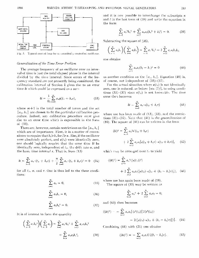
Figure 3 shows a block diagram of a typical standard of the passive type. An equivalent diagram of this frequency-lock servo is shown in Fig. 4, where Vl(w) is the Fourier Transform of the noise generated in the detec- tors, associated demodulating circuitry, and the frequency multipliers of Fig. 3. V z ( w ) is an equivalent noise voltage driving the reactance tube in the oscillator to produce the i ( t A ) term in the unlocked oscillator, such tha t flicker noise FM results. The power spectrum of Vz(w), then, is given by

where h , / / w l is the power spectral density of the fre- q u e n c y fluctuations of the unlocked oscillator.

I t is easiest to treat the servo equations by the use of the variable +, defined to be the difference between the output frequency of the multiplier and the “ideal” frequency of the atomic transition (the output of the “atomic device,” as shown in Fig. 4, is then assumed to be the constant zero). In order to preserve the dimensions of voltage for the addition networks, it is conve- nient to assume that the output of the subtraction net-

work is -/3+ \\.here p has the dimensions of volt- seconds. Thus, the equation governing the operation of the servo can be expressed, in the frequency domain, as

‘This leads to a pon-er spectral density for + given b!.

where use has been made of (54).

the order of 10 s-l. Thus, for small w , (56) becomes Normally, ~7~ becomes of the order of ( P N C ) for w of

1 S j ( W ) = -Sv1(w)

P (57)

RrnUtlCl YLLllPLlIR

X N

v, I w l NOl5E GENERATED IN DETECTOR Vz I w l E9UIVALENT NOISE TO GENERATE FLICKER NOISE IN VCC

Fig. 4. Eq~iivaleiit servotliagrarn oi‘ pnssikme type frccluenc.ystandard.

50

40

30

20

- in

2 0

U W in

a

0 IO a 5 8

B I 5

a 4

U

u s W

I

YI

E 3

2

I

I HOUR 3 HOURS I I

TIME (KILOSECONDS)

1;ig. 5. Liirixiice of dittereiices of the relative phase dilierence between two atomic standards.

2 16 PROCEEDINGS OF T H E IEEE FEBRUARY

0

1

2

By applying the techniques of Section I to the difference phase of t\vo cesium beams, the curves shown in Fig. 5 were obtained. Through least square fits to the data and comparing the ratios of the variances of differences (see Appendix), the result was obtained that the data fit curves of the form

-1 0

2 n + 1 12

- 2 n - 1 n + 1

for 7 = 1.34, \vi th a n uncertainty (standard deviation) of about +0.04. Again using [8] as before, this leads to the result that

tvhere p=0.34+0.04. One is, thus, led to the very strange conclusion thnt the spectral distribution of the detector and multiplier noise varies as - 1 w 1 The source of this noise a as later traced to a fault)- preampli- fier. With a proper aniplifier used, the spectral distribution appears white as other papers [SI, [ lo ] , [ l l ] indi- cate should be the case.

Ideally, for measurenients over times large compared to the servo time constant, the error accumulated during one measurement interval should be independent of errors accumulated during nonoverlapping intervals, i.e., mathematically analogous to Broxvnian Afotion [12] . This implies that S,(w) should be constant for Iw/ <1 s-1.

EXPONENT 7

Fig. 6. Ratio of variances, ((Anf1 m ) z ) , / ( ( A n m z ) z } , as a functioii of the exponent 7.

The Composite Clock System

If an oscillator's frequency is measured by an atomic standard, the error in measurement of the frequency is given by

1966 BARNES: ATOMIC TIl4EKEEPING A N I ) PKECISIOK SIGNAL GENER.A'l'OKS 217

I t is easl to shou that these coefficients satisf!. (35) (37).

Substitution of these coefficients into (47) qrields

((a/)?) = 2h?j -2rz'(2n + 1) In ( 1 1 )

+ 2(n + 1)"212 + 1) In ( 1 2 + 1)

- (2n + 1)' In (2n + 1) 1 , (61)

\\.here h = k 2 / 8 In 2. Since T is normally sniall compared to I * , it is reason-

able to approximate (61) for large n. Tha t is, the relative time error is approximately given by

\\here the approxiin, a t ' ions

1 In ( a ) + - IZ >> 1, In ( n + 1)

M

have been used. I t is apparent from (62) that for a given interval T, the errors accumulated by the clock are not critically dependent on the measuring time T , since dlF&] is a verq slo\\-Iy changing quantity.

The mean square error associated n i t h the standard, ho\\\-ever, can be ivritten in the form

since (59) may be written as the first difference of yn. From (57) it is apparent that the relative time error is then given by

where q = 1 (('white" noise). Or, combining (59), (62), and (64),

As one should expect, for a given 7', the errors get less for larger T but not rapidly. In the limit of T = 7' [not using the approxiniate (65)], the errors are those of the standard alone, i.e., 4 B 1 r / 2 ~ f S . ,Also, as 7 - 4 , the clock errors are unbounded.

Compounding Time Errors

Equation (65) represents a reasonable approxim a t ' ion to the time errors of a clock systeni after one calibration interval. The next question is: ho\v do the errors of niany calibrations compound to give a total error S(NI-) after N calibrations? Returning to (59), one ma\. n-rite

\\ here 6T, is the tinie error ,issoci,ited \\,it11 the nth calibration interval. 'There have been papers published [13] that assume that the errors of one calibration interval are not correlated to the errors of 'in) other c,tIibration interval. I t is no\\ possible to investigate this ,tssump- tion more precisell.

In particular, the clock errors (not including the frequency standard errors) 6t,, conipound to give S ( N t ) , given by

N

6(Av\) = at,,, n=l

n.hich can obviously be put in the forni of (41). I;or A7 equal to any number larger than one, the algebra becomes much too lengthy for actual calculation by hand and it is desirable to make use of a digital computer. 'Table 111 shows the results of this calculation for coni- pounding several third-difference-type calibrations. I t is interesting to note that, in fact, the total iiiean square error after N calibrations is very nearly equal to N - times the mean square error after one calibration. This is in quite good agreement kvith DePrins [ I S ] . Thus, the rnis relative eror may be approximated by the relation

jvhere h, n, B1, f?, and T have the same meanings as in (65).

TABLE I11 THEORETICAL D E T I ? K M I N A T I O N OF T I M E E R R O R PROPAG4TION

2.054 3.109 4.165 5.220 6.276 7.332

The conclusions which can no\\ be drawn are that : 1) the total rnis time error of this clock system from an "ideal" atomic clock is unbounded a s time increases, and 2) the relative rms error time to total elapsed tinie (6X) approaches zero about as fast as W1'2. I t should be mentioned here that systematic errors in the atomic standard have not been considered. II'hile this is a very important problem, it has been tre'ited rather thor- oughly elsewhere [ lo] , [ l l ] , [14]-[16].


I\’. RIEASUKES OF FREQUENCY S m r m I n

General liestrictions

I t is of value to consider the problem of establishing a stability nieasure in a very general sense. Consider some functional of the phase

x = x(4(t>)r

from nhich the stnbilit! iiiecisure q is obtained accord- ing to the re1 a t‘ 1011

q2 Lim -

provided this limit exists.

and, thus, one iiieasures for soiiie fixed tinie, 1‘; i.e., In practice it is riot possible to pass to the limit T-+ 00,

I’nder favorable conditions, \k7! may be a reasonable approxiniation to \k. IJnfortunately, this may not al- a a y s be the case.

The frequenc) emitted by any physically realizable device rriust be bounded by some upper bound, sal- B. The folloLving inequalities must, then, be valid :

I n(t) I 5 B, for some B > 0;

Lim - T i 2 ( 1 2 ( t ) ) 2 dt 5 B2. T - m T

With S;(w) being the pouer spectral densit!, of Q ( t ) , it follo\vs from the definition of pou-er spectra that

Lim - T ’ 2 (n(t ) )? d! = 2 L = S i ( w ) dw T - m T - ~ , 2

for real Q ( t ) , and thus

2 sgisb(w) dw 5 B?. (69)

If S,(w) has a flicker noise spectrum for small w , it is apparent that this l / l w l type of noise cannot persist to absolute zero frequency or the inequality (69) would be violated. I t is, thus, reasonable to postulate the existence of a loner cutoff frequency 01, for the flicker noise modulation.

I t is apparent from the preceding considerations that stability measures may exist for u hich q.1, begins to approach q onlS. after T is several times larger than 1/wL. From some of the experiments 04 crystal oscillators [ 2 ] , this may require 1’ to exceed several years in duration. This is quite inconvenient from a manufactur- ing or experimental standpoint. The logical conclusion is to consider only those stability measures \k \vhich are “cutoff independent,” that is, those measures of stability which Lvould be valid even in the limit wL-+O+.

6

Finite Di ferences

form I t \vas shoivn in Section I1 that an expression of the

1 m 1 ..-

61 = - E a&(t + bnr) a0 n=O

will have a finite variance if the {a , , b,i 1 satisfy conditions (35)-(37). I t is easy to shoi\ that the first difference of the phase (Le., frequent>) cannot be put in the forni of (70) \vith the coefficients satisfying conditions ( 3 5 ) - (37). Indeed, the limit

does not exist, and, hence, C r ( 7 ) is not a good nieasure of stab i 1 it y .

The variances of the second and third finite differences, hmvever, are convergent. I t is of interest to note that the first line of Table 111 may be expressed in the forni

which may be simplified to the forni

This equation expresses the fact t ha t a third difference has a very small correlation (-3 percent) to an adjacent, nonoverlapping third difference. I3). extending this procedure v i th the other values given in Table 111, it is found that the correlation of one third difference with a nonoverlapping third difference beconies sniall very rapidly as the interval between these differences becomes large. This is sufficient to insure that the variance of a finite sample of third differences mill approach the “true” variance (infinite average) in a well-behaved and reasonable fashion as the sample gets larger.

Variance of Frequency Fliictiiations f o r Fini te Averaging Times

Even though the variance of the first difference of the phase does not satisfl. the condition of being cutoff independent, it is possible (by specifying both the sample time and the total averaging time) to construct a cutoff independent measure of the frequency fluctuations. Instead of \kT, the variance of N adjacent samples of the frequency will be denoted by a2(r , N ) m-here T is the sample time for each of the Ai measurements of frequency. The variance is given by the conventional f orin ula

1966 BARNES: ATOlIIC TI l lEKEEPISG AND PKECISIOK SIGNAL GENERATORS 2 19

I f one neglects the drift rate a , \\-hich is essentiall>. equivalent t o obtaining the standard deviation around ;I linear drift, one obtains

1

!I7 - - ( [ E ( t + iVT) -

For the case of an “ideal” cr1,stal oscillator, (19), (24), and (26) allow (71) to be simplified (after passing to the l ini i t p-+l(-) to the form

2 h S In (S)

s - 1 ( d ( 7 , S)) = ___----

,. I hus, as N increases, the expected value of u2(7, N ) i n - creases ni thout bound (at least until ; V T - ~ ’wL ) . I t is interesting to note tha t for ‘1 given oscillator, ( ~ ~ ( 7 , 1%’) i has a mininiuni value for N = 2 . Obviousl) one would have to average several experimental determinations of d ( ~ , 2) in order to have a reasonable approximation to

\Vhile ~ ( 7 , N ) is a cutoff independent measure of frequency stabilit) , it has the significant disadvantage of being a function of t n o variables. Indeed, in order t o conipare the stabilitj. of t u o oscillators, both the 7 ’ s and the N ’ s should have nearly corresponding values

(CY77 2)) .

Delayed Frequency Comparison

In radar n-ork, often the frequent) of a signal is coni- pared to the frequency of the smie source after i t has been delayed in traversing some distance-often a very great distance. One might, thus, be interested in defining it stability measure in an analogous fashion:

7

( 7 2 ) - _______.

T

rlg<Lin neglecting the drift rate a of the oscillator, (24) mid (72) combine to yield

1 *’(T, T ) = -; [21~(7 ) - - . (T -T)+21 . (T ) - - . (T+T)] . (73)

T-

I f te r substitution of (26) into (73) the e q u t i o n can tie rearrmged to give (again passing to the liniit, p+l(-’)

\lr?(r, T ) = - 2 1 i [ p ? I n p - (1 + p)’ In (1 + p )

- ( p - 1): I n ( p - l ) ] ,

\\ here p = 2’ ’7. >4lthough this is a rather coniplicated es- pression, it ma) tie sirnplified I\ i t h the approximation p - T ” T > > ~ . The result is

T

for a n “ideal” oscillator. I t is interesting to note here that even \\ hen considering on11 1 j w 1 t) pe of noise, one cannot pass to the liinit T = O for this probleni. In the limit as T+O+, the expression

and thus

Lim !P?(T, T ) = ( [ Q ( t + T ) - Q ( L ) ] ~ ) ---f 3 ~ . 7-0+

from (74), even though 7’<<1 / w L . The source of this difficult1 is the high-frecluenc> divergence of the flicker noise spectrum. If the SE stem is limited a t the high frequenc) by w I f , then one should pass to the liniit 7-1 ’wI I .

Xg‘iin, $ ( T , 7 ) is a function of t\\ o variables I\ i th all of the associated .inno) arices. I t m a > , hou ever, be useful in certain applications.

Conc L I SIOh

The assuinptions of stationarit) .ind “idelil” behnvior for quartz cr! stal oscillntor lead to <L statistical model I\ hich agrees I\ ell \I ith iiian> different experiments One finds, hon ever, tha t certnin qu,intities ‘ire 1111- hounded ‘1s ,Lveraging times are extended and it is iiii- portant to consider on11 those quantities 11 hich hnve reasonable hope of converging to\\ ard <i good value in reasonable time. Thus, the concepts of cutoff dependent and cutoff independent measures of frequent) stabilit> form a natural classification for a l l possible frequencx stabilits nieasures.

On the basis of “ideal” behavior, i t has been shovn tha t the errors of a clock, run from ‘L quartL crystal oscillator and periodical11 referenced to a i atomic frequenc) stnndard, accumulate error at <i probable rate proportional to the square root of the number of calibr,i- tions. That IS , the errors of one calibration interval <ire essentiall) uncorrelated to errors of nonoverlapping intervals in spite of the fact th,tt “idecil” beh,ivior is highl! correlated for long periods of time

I t has also been shonn that the method of finite differences can be a useful method at determining spectr,il distributions of noise, ‘1s \\ell AS being ‘i possible niecisure of frecliienc> stahilit! I3x using higher order finite differences, phase fluctuations I\ ith even a higher order pole a t Lero-modulation frequencv can siniilarlj be treated The need for hiqher than second or third differences, hou ever, has not 3 e t been deiiionstr<ited.

I t should be noted tha t the existence of higher-frequenc) nioduLition noise of different origin ,ilso h,is significant affect on st,tbilitj nieasures. 111 gerier,tl, the factors hich l i i i i i t the sx stem to ‘i hnite bmdpciss ,ire sufficient to insure convergence of the stabilitx iiie‘isures as w+ x: If it is primnril> the me,isuriiig SJ stein I\ hich limits the sx stem bandpass, hou ever, the results m,i> be significantl> altered bjr the ineasuring q steni itself.

220 PROCEEDINGS OF THE IEEE

APPENDIX

R.1 I IO OF \‘.\KIANCES

Let ~ ( t ) be a real generalized function such tha t ( t ( t ) )

= O and define the discrete variable E, by the relation

tm E t ( t + WlT). (75)

.Also, let the auto-covariance function of ~ ( t ) be, as before, independent of a simple time transition. One [nay IIOR. \trite (see Table I j

((Ae,,)’) = 2 [ ( ( c , , ) ? ) - ( [ e ( / + T ) E ( t ) ] ) ] (76)

and assume t h a t ((AEm)2) = R I T ? , (77)

lvhere kl is a constant for ‘1 given 7. I t is also possible to obtain the varinnce of the second difference:

((LI?~,)~) = 6((tm,)2) - 8([t(t + T ) . E ( ~ ) ] )

+ ( [ 4 t + 2T) t ( t ) l ) . (78)

I-sing (77) and ( 7 X ) , one nia? obtain

Since (79) must be non-negative (e is real), the exponent is restricted to the range 7,752.

Siinilarl>,, one maj. obtain the variance of the third difference

a n d hence the ratio

Si m ilarl j-,

Equations (79), ( X l ) , and ( 8 2 ) are plotted in Fig. 6 as a function of the exponent 7 .

For q = 4 3 , ;is in Fig. 6, the theoretical ratios,

( ( ar1+ I&) 9 )

for n = l and 2 are 1.48 and 2.84, respectively. The straight lines dran-n in Fig. 5 were made to have these ratios and slope 2 ’ 3 (the square root of the variances).

.~CK?~TOWI,EDGMENT

The author is sincerely indebted to Urs. 1’. Wacker and E. Croiv of the National Bureau of Standards for soiiie very valuable suggestions and references. The author also Lvishes to acknoa-ledge the assistance of D. ,Allan for his aid in data acquisition and analysis, R. E. Beehler for making the cesium beams of the N D S available, and R. I,. Fey for some helpful criticism.

REFEKEXCES [I] H. Lyons, “The atomic clock,” Ani. .%kolar, vol. 19, pp. 159-

168, Spring 1950. 121 \\’. li. Arkinsoii, I*. Fey, and 1. Newmnn, “Spectriim anal~-siis

of extremely low frequency vnri;itions of quartz oscillators,” Pror. IEEE (Correspondenre), vol. 51, p. 379, February 1963.

131 I,. Fey, ,\\.,, R. Atkinson, and J . I-ewmaii, “Obscurities of oscillator noise, Pror. IEEE (Correspondenre), vol. 52, pp. 104-105, January 1964.

[l] V. Poitsky, “Certain problems of the theory of fluctriations iii oscillators. The iiifluetice of flicker noise.” IZ‘L,. Vvsshikh 1’rWebn. Zaoedenii, Radiojir., vol. 1 , pp. 20-33, 1958.

[ S ] I,. Cutler and C. Searle, “Some aspects of the theory and measureinent of frequency fluctuations i n frequent)- standards,” this issue, page 136

[6] J . A. Barnes and l i . C. MoclJer, “The power spectrum and its imnortance i n precise freciueiics ineasureinents.” IRE Tranc on Instrumentntioh, vol. 1-9, ‘pp. 129-155, September 1960.

[7] K. \Yiener, Ewtrapolafion, Interpolation, and .SwzootkinE o j Sta- tionary Time Series. Cambridge, hlass. : Techuology Press of Mass. Iiist. of Tech., and New York: \!?ley, January 1957.

[8] SI. L.ighthill, Introdmtion to Fourier A n d Functions. New York: Cambridge, 1962.

[9] Is. R. Malling, “Phase-stable oscillators for space coiiitnu~~ica- tions, including the relationship between the phase noise, the spectrum, the short-term stability, and the Q of the oscillator,” Proc. I K E , vol. 50, pp. 1656-1661, July 1962 (see also [%?I).

[ IO] P. Kartaschoti, “Influence de I’effet de greriaille stir la frequence d’un oscillateur asservi R 1111 eta1 on a jet atomique,” Laboratoire Suisse de fiecherches Horlogeres, Neuchatel, Switzerland, No.

[ I l l P. Kartascbpff, “Etude d’un etalon de frequence a jet atomique de cesium, Laboratoire Suisse de Iiecherchess Horlogeres, Neuchatel, Switzerland. November 1963.

1121 S. Basri, “Time standards and statistics,” to be published. [I31 J . DePrins, “Applications des masers A N15H:j a la mesure e t ;I

In definition du temps,” unpublished Doctor of Sciences disserta- tion, Uiiiversite‘ Libre de Bruxelles, Belgium, 1961.

[14] R. E. Beehler, LV. I<. Atkinson, L. E. Heiin, and C. S. Snider, ‘‘A comparison of direct and servo methods for utilizing cesium beam resonators as frequency standards,” IRE Trans. o n In- strumentation, vol. 1-1 1 , pp. 231-238, December 1962.

1151 13. E. Beehler and I). J . Glaze, ‘ T h e perforriiance and capability of cesium beam frequency standards a t the National Bureau of Standards,” to he published.

[16] R. E. Beehler and D. J . Glaze, ”Evaluation of a thallium atomic beam frequericy standard a t the National Bureau of Standards,” to be published.

08-64-01.

atomic timekeeping and the statistics of precision … august 1960. ire, voi. 48, pp, 1167-1473,...

Documents