attosecond dynamics in molecules and on interfaces · attosecond dynamics in molecules and ... one...
TRANSCRIPT
Attosecond Dynamics in
Molecules and on Interfaces
Dissertation
von
Michael Jobst


Fakultät für Physik
Laser– und Röntgenphysik
Attosecond Dynamics in Molecules
and on Interfaces
Michael Johannes Jobst
Vollständiger Abdruck der von der Fakultät für Physik der Technischen
Universität München zur Erlangung des akademischen Grades eines Doktors der
Naturwissenschaften genehmigten Dissertation.
Vorsitzender: Univ.- Prof. Dr. Ulrich GerlandPrüfer der Dissertation:Univ.- Prof. Dr. Reinhard KienbergerUniv.- Prof. Dr. Matthias RiefDie Dissertation wurde am 03.12.2014 bei der Technischen Universität Müncheneingereicht und durch die Fakultät für Physik am 18.12.2014 angenommen.

Abstract
In this thesis three experimental approaches to the measurement of electronic move-ment on the attosecond time scale in complex systems are presented. The first chapterdescribes the basic theory and technology necessary for these endeavors as well as theactual equipment used and refined during this thesis.The subsequent chapters present the experiments on three different types of systems:molecules in the gas phase (specifically ozone), molecules on surfaces (metal-organicmolecules on semiconductors) and metal surfaces and interfaces (tungsten in two crystalorientations and oxygen on tungsten).The first of these three chapters begins with a report on the development of a highpurity ozone source. The creation of ultrashort deep UV pulses (ca. 220 nm–300 nm)through frequency tripling for pump probe experiments and the suppression of the NIRfundamental light is described. The combination of UV and isolated XUV pulses in anexperiment is realized and demonstrated on ozone. An overview over the current theoryon electron dynamics in ozone in the Frank–Condon region is given and complementedwith the current status of the time dependent measurements.The second chapter focuses on the sample choice for the detection of a time dependentchemical shift in photoelectron spectroscopy experiments with metal-organic moleculeson semiconductor surfaces. Observation of the metal center as well as iodine tagging forimproved XUV sensitivity are explored.In the third chapter the recent measurements of attosecond delays between photoelec-tron emission from the tungsten 4f and valence levels are described. In a first step theextension of the experimentally usable XUV spectrum up to energies of 150 eV is re-ported, then streaking measurements at 145 eV photon energy are demonstrated. Themultitude of theoretical explanations for the origin of photoemission delays in tungstenis summarized and compared with experimental results. Delay measurements at 145 eVand their results on W(110), W(100) and oxygen on tungsten are presented. A synthesisof all measurements on clean tungsten, oxygen on tungsten and hydrogen on tungstenthat have been performed before and during this thesis is given.At the end of every chapter there is a section containing conclusions and an outlook forthe respective experiments.
v

Kurzzusammenfassung
Im Rahmen dieser Arbeit werden drei experimentelle Ansätze zur Messung von Elektro-nendynamik auf der Attosekunden Zeitskala präsentiert. Das erste Kapitel befasst sichmit der zu Grunde liegenden Theorie, Technologie und den für diese Arbeit verwendetenund verbesserten Geräten.Die darauf folgenden Kapitel präsentieren Experimente an drei verschiedenen Klassenvon Systemen: gasförmige Moleküle (Ozon), Moleküle auf Oberflächen (metallorganischeMoleküle auf Halbleitern) sowie Metall Oberflächen und Grenzflächen (Wolfram in zweiverschiedenen Kristallorientierungen und Sauerstoff auf Wolfram).Im ersten dieser drei Kapitel wird zunächst die Konstruktion einer Quelle für hochreinesOzon beschrieben. Die Herstellung von ultrakurzen Pulsen für Anrege Abfrage Experi-mente im tiefen UV (ca. 220 nm–300 nm) durch Frequenzverdreifachung von NahinfrarotPulsen wird erläutert. Die Kombination von Attosekunden XUV Pulsen und Femtosekun-den UV Pulsen in einem Experiment wird gezeigt. Die hierfür nötige Unterdrückung desNahinfrarot Treiberpulses wird behandelt. Die relevante Theorie zur Elektronendynamikin Ozon in der Frank–Condon Region wird präsentiert und deren Ergebnisse mit demmomentanen Status der zeitaufgelösten Messungen verglichen.Das zweite der experimentellen Kapitel konzentriert sich auf die Auswahl einer vielver-sprechenden Probe für die Detektion einer zeitabhängigen chemischen Verschiebung inPhotoelektronen Experimenten an metallorganischen Molekülen auf Halbleiter Ober-flächen. Die direkte Detektion durch Beobachtung des Metall Zentrums sowie eine indi-rekte Messung an Molekülen, die mit Jod Atomen markiert wurden, wird diskutiert.Im dritten Kapitel werden die jüngsten Attosekunden Messungen zur Verzögerung derPhotoemission zwischen den Wolfram 4f und Valenz Niveaus beschrieben. Zunächst wirdüber die Ausweitung der erreichbaren Photonenenergie berichtet. Streaking Messungenbei 145 eV werden demonstriert, wobei das Photonen Spektrum sich bis mindestens 150 eVerstreckt. Die theoretischen Ansätze zur Erklärung der gemessenen Verzögerungen wer-den zusammen gefasst und mit experimentellen Resultaten verglichen. Verzögerungsmes-sungen an W(110), W(100) und Sauerstoff auf Wolfram werden gezeigt. Ein Überblicküber alle bisher erfolgten Messungen an sauberem Wolfram, Sauerstoff auf Wolfram undWasserstoff auf Wolfram wird gegeben.Zu Ende jedes Kapitels befinden sich sowohl eine Zusammenfassung der jeweiligen Ex-perimente als auch der zugehörige Ausblick.
vii


Contents
1 Introduction 1
2 Experimental and Theoretical Tools 72.1 Principles of Attosecond Experiments . . . . . . . . . . . . . . . . . . . . . 7
2.1.1 Few Femtosecond Pulses . . . . . . . . . . . . . . . . . . . . . . . . 72.1.2 Generation of Isolated Attosecond Pulses . . . . . . . . . . . . . . 82.1.3 Streaking . . . . . . . . . . . . . . . . . . . . . . . . . . . . . . . . 112.1.4 Generation of Ultrashort UV Pulses . . . . . . . . . . . . . . . . . 152.1.5 Measurement of Femtosecond Pulses: FROG . . . . . . . . . . . . 15
2.2 Equipment . . . . . . . . . . . . . . . . . . . . . . . . . . . . . . . . . . . 172.2.1 The Laser System: FP3 . . . . . . . . . . . . . . . . . . . . . . . . 172.2.2 The Surface Science Beamline: AS3 . . . . . . . . . . . . . . . . . 232.2.3 The Interferometric Beamline: AS2 . . . . . . . . . . . . . . . . . . 27
3 Molecules in the Gas Phase: UV/XUV Pump Probe Experiments in Ozone 293.1 Principle of the Experiment . . . . . . . . . . . . . . . . . . . . . . . . . . 29
3.1.1 Time Resolution versus Energy Resolution: The Choice of XUVMirror . . . . . . . . . . . . . . . . . . . . . . . . . . . . . . . . . . 29
3.2 Sample Preparation: Ozone Distillation . . . . . . . . . . . . . . . . . . . 303.3 UV Generation and IR Suppression . . . . . . . . . . . . . . . . . . . . . . 32
3.3.1 UV Generation . . . . . . . . . . . . . . . . . . . . . . . . . . . . . 323.3.2 IR Suppression . . . . . . . . . . . . . . . . . . . . . . . . . . . . . 37
3.4 Calculations and Expected Experimental Results . . . . . . . . . . . . . . 403.4.1 Full-fledged Quantum Calculations . . . . . . . . . . . . . . . . . . 403.4.2 Three Level Calculations . . . . . . . . . . . . . . . . . . . . . . . . 44
3.5 Time Resolved Photoelectron Spectroscopy on Ozone . . . . . . . . . . . . 453.5.1 IR Pump, XUV Probe . . . . . . . . . . . . . . . . . . . . . . . . . 453.5.2 UV Pump, XUV Probe . . . . . . . . . . . . . . . . . . . . . . . . 47
3.6 Conclusions . . . . . . . . . . . . . . . . . . . . . . . . . . . . . . . . . . . 473.7 Outlook . . . . . . . . . . . . . . . . . . . . . . . . . . . . . . . . . . . . . 49
4 Metal–Organic Molecules on Surfaces 514.1 Principle of the Experiment . . . . . . . . . . . . . . . . . . . . . . . . . . 514.2 Sample Choice . . . . . . . . . . . . . . . . . . . . . . . . . . . . . . . . . 51
4.2.1 The Substrate . . . . . . . . . . . . . . . . . . . . . . . . . . . . . . 534.2.2 The Molecule . . . . . . . . . . . . . . . . . . . . . . . . . . . . . . 53
ix

Contents
4.2.3 Sample Preparation . . . . . . . . . . . . . . . . . . . . . . . . . . 554.3 Steady State Experiments . . . . . . . . . . . . . . . . . . . . . . . . . . . 55
4.3.1 Direct Observation of the Metal Center: Os2172 . . . . . . . . . . 554.3.2 Iodine Tagging: MBM4179 . . . . . . . . . . . . . . . . . . . . . . 584.3.3 Iodine Tagging and Evaporation Deposition: Tetraiodo Copper Ph-
thalocyanine . . . . . . . . . . . . . . . . . . . . . . . . . . . . . . 604.4 Conclusions . . . . . . . . . . . . . . . . . . . . . . . . . . . . . . . . . . . 644.5 Outlook . . . . . . . . . . . . . . . . . . . . . . . . . . . . . . . . . . . . . 64
5 Attosecond Delay Spectroscopy on Tungsten 655.1 Principle of the Experiment . . . . . . . . . . . . . . . . . . . . . . . . . . 655.2 Theoretical Considerations . . . . . . . . . . . . . . . . . . . . . . . . . . . 675.3 Past Measurements on Tungsten and O/W . . . . . . . . . . . . . . . . . . 695.4 Production and Characterization of High Harmonics at 145eV . . . . . . . 725.5 Delay Spectroscopy of Tungsten and O/W at a Photon Energy of 145eV . 73
5.5.1 Clean Tungsten 110 . . . . . . . . . . . . . . . . . . . . . . . . . . 735.5.2 Clean Tungsten 100 . . . . . . . . . . . . . . . . . . . . . . . . . . 785.5.3 Measurements on O/W . . . . . . . . . . . . . . . . . . . . . . . . 78
5.6 Overview of Delay Measurements on Tungsten . . . . . . . . . . . . . . . . 815.7 Conclusions . . . . . . . . . . . . . . . . . . . . . . . . . . . . . . . . . . . 815.8 Outlook . . . . . . . . . . . . . . . . . . . . . . . . . . . . . . . . . . . . . 83
Bibliography 85
6 Acknowledgement 97
x

Chapter 1
Introduction
Electronic motion on the Angstrom length scale is a fundamental process that drives awide variety of phenomena from chemical bond rupture to photosynthesis. In order totruly understand the evolution of these microscopic phenomena one needs to trace thecharges as they are moving, which can demand an extremely high temporal resolution.Microscopic motion is determined by the evolution of coherent superpositions of electronicstates (wavepackets). The time scale of the dynamics of these wavepackets is given byh/�E, where h is Planck’s constant and �E is the energy separation of the levels involvedin the formation of the wavepacket. The typical energy scale of valence electron dynamicsis known from spectroscopy to be in the range of a few electron volts. This translatesto a time scale in the range of attoseconds (1 as = 1⇥ 10�18 s) to few femtoseconds(1 fs = 1⇥ 10�15 s). This time resolution has only been available for little more than adecade [1] and so it comes as no surprise that a significant part of the research performedso far focused on the development and refinement of experimental techniques. In thefollowing section an overview over selected approaches to study electronic motion on anultrashort timescale is given.
Attosecond Experimental Techniques
In order to get experimental access to the electron dynamics we need a time gating mech-anism on the attosecond scale: either be a process internal to the sample or an externallyapplied field.One technique that uses an internal process is the Core Hole Clock [2]. It can for ex-ample be used to measure charge transfer times in dielectric adsorbates on metals andis typically performed in synchrotron facilities where tunable and intense X–ray pulsesare available. When the sample is exposed to the X–ray beam, a photon excites a coreelectron of the adsorbate and creates a core hole. The hole is filled within its character-istic lifetime and simultaneously the charge transfer process from the excited state of theadsorbate to the surface takes place. In an autoionization process an electron is ejectedfrom the adsorbate and subsequently detected. The ratio between the lifetimes of theexcited state and the core hole can be calculated from the kinetic energy distribution ofthis electron when the photon energy is varied. If the core hole lifetime is very short,well known and comparable to the exciton lifetime it is possible to achieve attosecondtime resolution, which was demonstrated by Föhlisch et al. for sulfur on ruthenium [2].We can conclude that the core hole clock is a powerful method for the measurement of
1

Chapter 1 Introduction
charge transfer times, but it does require quite specific properties from the sample inorder to be usable.From here on we will focus on approaches utilizing externally applied field gradients,which promises greater versatility. The key towards a much higher time resolution lies intaking the step from the envelope of the laser field to the oscillating electromagnetic fieldof the laser. This is achieved by controlling the carrier envelope phase1 (CEP) with thetechnology pioneered by Udem et al. [3]. For few cycle pulses2 changes in CEP affect thetemporal shape of the electric field significantly. The combination of few cycle pulses andCEP stabilization yields control over temporal field gradients on the attosecond timescale[4].Few cycle pulses in the near infrared (NIR) range are used for a variety of different ex-periments, among which we have selected three to present here. The first example is theattoclock [5]. In this setup an intense circularly polarized few cycle laser pulse is used tophotoionize helium atoms. From the radial distribution of the resulting photoelectronsEckle et al. draw conclusions about a lower bound to the tunneling time of the photoelec-tron [6]. While the interpretation of this measurement is challenging [7] it does provideinformation about electron dynamics on a very short timescale.Another noteworthy experiment is the investigation of nonsequential double ionization[8]. Bergues et al. report a strong CEP dependent correlation in the electron emissionfrom argon when double ionized with few cycle laser pulses–a clear signature of ultra-fast multielectron dynamics. For this experiment the carrier envelope phase was notstabilized– but it was measured for every single laser shot [9]. Then the acquired datawas mapped to the phase and revealed the CEP dependence.In both of the just mentioned publications the scrutinized effect depends nonlinearly onthe electric field. This is not a coincidence but a necessary property when employing fewcycle pulses for attosecond time gating. The contrast in field strength between the twomost intense field peaks is only about 1.3 for even the shortest conventionally achievablepulses. If the studied effect depends exponentially on the field strength (as tunnelingdoes) the effective time contrast is enhanced such that the effect is limited to an attosec-ond interval within the most intense optical cycle.The third example is high harmonic spectroscopy (HHS) [10]. When gas atoms are sub-jected to an intense laser field they can go through a three step process: ionization,acceleration of the released electron away from and then back to the ion in the revers-ing laser field, and recombination of the accelerated electron with the parent ion [11].The energy accumulated in the field is released as a soft X–ray (or extreme ultra violet,XUV) photon. Since the returning electron is well defined in space and time one can inprinciple extract information with Angstrom spatial and attosecond temporal resolutionfrom the resulting photon spectrum. In fact, there have been reports on tomographicmeasurements of molecular orbitals [12], vibrational excitations [13] and even chemicalreactions [14]. HHS is often labeled as a pump–probe type experiment. In this picture the
1The carrier envelope phase describes the phase of the light oscillations within the envelope. For a CEPof 0 or ⇡ the maximum of an oscillation coincides with the envelope maximum.
2Pulses that are so short that they containing less than two field oscillations
2
ionizing laser field represents a pump pulse (starting the dynamics of interest) while thereturning electron takes the role of the probe (reading out the properties of the system).In a standard pump–probe experiment the temporal evolution of a system is studied byscanning the time delay between the two pulses. For HHS the time delay is determinedby the oscillation period of the driving laser (i.e. the central wavelength), which is eitherchallenging or impossible to change significantly.
Attosecond Pulses
In order to perform pump–probe experiments in the conventional sense attosecond pulsesare necessary. It has been shown that the XUV pulses that are used as an observable inHHS can serve this purpose. If the high harmonic generation (HHG) process is performedwith a long driving pulse (containing significantly more than two field oscillations) theharmonics will form pulse trains spaced in time by half an oscillation period of the drivinglaser. Due to the high photon energy of the XUV pulses they offer access to electronsbeyond the valence shell and enable the measurement of dynamic chemical shifts of corelevels [15]. Of course the time resolution for pulse trains is limited by the duration ofthe train, not the individual pulses. If intense few cycle pulses are used to drive theHHG process and the resulting radiation is carefully manipulated, one can obtain iso-lated XUV pulses as short as 67 as [16]. Two of the ways in which isolated attosecondXUV pulses can be applied in pump–probe experiments will be presented here. The firstone is called attosecond transient absorption spectroscopy (ATTAS), the second one isattosecond photoelectron spectroscopy (APS).For ATTAS, the XUV probe beam is focused onto the sample, is transmitted throughit and then analyzed with a spectrometer. Absorption lines of the sample that overlapwith the XUV spectrum are detected as dips in the spectral intensity. As the delaybetween NIR pump and XUV probe beam is varied one can draw conclusions about thepopulation of electronic states from the temporal evolution of these dips. One beneficialproperty of ATTAS is the fact that the time and energy resolution are not coupled. Thetime resolution of ATTAS is limited by the pulse length of the XUV probe pulse. Evenif the driving pulse is longer than the probe pulse it is still phase locked and thus theoptical field is identical for every pulse. The XUV pulse can then read out the evolutionof the sample within the electric field with attosecond resolution. The spectral resolu-tion is limited by the employed spectrometer–not the spectral resolution of NIR or XUVpulses. Due to this the ATTAS method can be used to study slow processes (for whichhigh spectral resolution is necessary) and fast processes (requiring high temporal reso-lution) simultaneously. It has been used to measure valence electron motion in kryptonatoms [17] and showed that strong–field ionization can produce long lived coherences.The method is also applicable to thin solids as was shown by Schultze et al. [18] whoscrutinized the change in the electronic structure of fused silica exposed to intense laserradiation.The second experimental ansatz utilizing isolated XUV pulses is attosecond photoelectronspectroscopy (APS). This approach is used for all experiments presented in this thesis.In APS the XUV probe pulse ionizes the sample, thereby releasing photoelectrons which
3

Chapter 1 Introduction
are subsequently detected and analyzed. In contrast to ATTAS no resonance overlap-ping with the XUV spectrum is necessary and APS is applicable to a very broad range ofsamples. One merely needs an appreciable absorption cross section in the energy rangeof the XUV pulse. The temporal and spectral resolution of APS are both limited by thesame quantity: the bandwidth of the XUV pulse. This means that compromises haveto be made when determining the appropriate bandwidth for the specific experiment.At the currently achievable photon energies APS cannot be used to study dynamics inbulk solids because photoelectrons with the kinetic energies typically produced by XUVpulses have a mean free path in solids of only a few Angstrom. Only the photoelectronscreated within a few layers from the surface can escape the solid and be detected. Onthe other hand APS is very well suited for surface dynamics.There is a special variant of APS, called streaking, which essentially measures a crosscorrelation between the photoelectrons and the NIR laser field [1]. It can provide infor-mation on the release time of photoelectrons relative to the driving field with a precisionof less than ten attoseconds as demonstrated in neon gas [19]. The method is also appli-cable to monocrystalline, polycrystalline and amorphous solids [20, 21]. A particularlyintriguing experiment on a complex layered sample was performed by Neppl et al. [22].The authors fabricated a tungsten crystal with a monolayer of magnesium on top. Theythen varied the thickness of the adlayer between one and four atomic layers and measuredthe corresponding emission delay between the tungsten 4f level and the magnesium 2plevel. They found the delay to increase linearly with the adlayer thickness, which is adirect measurement of two effects:
• electronic transport on the attosecond and angstrom scale through the magnesiumlayer.
• dielectric screening on the angstrom scale at the vacuum/magnesium interface. Theobserved increase in delay can only be explained with a vanishing penetration depthof the NIR streaking field into the magnesium.
Current Advances in Attosecond Dynamics in Molecules and on Interfaces
As mentioned in the first paragraph of the introduction, new experimental techniqueshad to be developed for many exciting findings in attosecond science so far. But nowthis branch of ultrafast physics matures and there are an increasing number of reportson applications of tried and tested methods exploring new samples or refining previousfindings. The three projects presented in this thesis form a microcosm of this evolu-tion. In the first project one we explore a new experimental ansatz–the combinationof deep UV pulses and APS on ozone. For the second one we study a very complexsample: molecular layers on surfaces. And for the third one we synthesize and expandprevious photoemission delay measurements on tungsten. These three experiments aresummarized in the following paragraph.
• Attosecond photoelectron spectroscopy of electron dynamics in ozone triggered bydeep UV pulses.
4
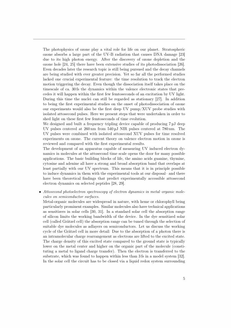
The photophysics of ozone play a vital role for life on our planet. Stratosphericozone absorbs a large part of the UV-B radiation that causes DNA damage [23]due to its high photon energy. After the discovery of ozone depletion and theozone hole [24, 25] there have been extensive studies of its photodissociation [26].Even decades later the research topic is still being pursued and the decay channelsare being studied with ever greater precision. Yet so far all the performed studieslacked one crucial experimental feature: the time resolution to track the electronmotion triggering the decay. Even though the dissociation itself takes place on thetimescale of ca. 30 fs the dynamics within the valence electronic states that pre-cedes it will happen within the first few femtoseconds of an excitation by UV light.During this time the nuclei can still be regarded as stationary [27]. In additionto being the first experimental studies on the onset of photodissociation of ozoneour experiments would also be the first deep UV pump/XUV probe studies withisolated attosecond pulses. Here we present steps that were undertaken in order toshed light on these first few femtoseconds of time evolution.We designed and built a frequency tripling device capable of producing 7 µJ deepUV pulses centered at 260 nm from 540 µJ NIR pulses centered at 780 nm. TheUV pulses were combined with isolated attosecond XUV pulses for time resolvedexperiments on ozone. The current theory on valence electron motion in ozone isreviewed and compared with the first experimental results.The development of an apparatus capable of measuring UV induced electron dy-namics in molecules at the attosecond time scale opens the door for many possibleapplications. The basic building blocks of life, the amino acids guanine, thymine,cytosine and adenine all have a strong and broad absorption band that overlaps atleast partially with our UV spectrum. This means that it is in principle possibleto induce dynamics in them with the experimental tools at our disposal– and therehave been theoretical findings that predict experimentally accessible attosecondelectron dynamics on selected peptides [28, 29].
• Attosecond photoelectron spectroscopy of electron dynamics in metal–organic mole-cules on semiconductor surfaces.Metal-organic molecules are widespread in nature, with heme or chlorophyll beingparticularly prominent examples. Similar molecules also have technical applicationsas sensitizers in solar cells [30, 31]. In a standard solar cell the absorption rangeof silicon limits the working bandwidth of the device. In the dye sensitized solarcell (called Grätzel cell) the absorption range can be tuned through the selection ofsuitable dye molecules as adlayers on semiconductors. Let us discuss the workingcycle of the Grätzel cell in more detail: Due to the absorption of a photon there isan intramolecular charge rearrangement as electrons are lifted to the excited state.The charge density of this excited state compared to the ground state is typicallylower on the metal center and higher on the organic part of the molecule (consti-tuting a metal to ligand charge transfer). Then the electron is transferred to thesubstrate, which was found to happen within less than 3 fs in a model system [32].In the solar cell the circuit has to be closed via a liquid redox system surrounding
5

Chapter 1 Introduction
the semiconductor substrate. Our object of interest is the hithertho unexplainedvery first step: intramolecular charge rearrangement. We study the dynamic chem-ical shift of core electrons in a selected atom within the metal–organic molecule asa proxy to the charge density in its vicinity and its temporal evolution.This is the first experiment with molecular layers on surfaces with our setup. Tran-sitioning from crystalline solid samples to molecule layers promises a drasticallylower signal and naturally our first step is the choice of a detectable sample. Wedetermine whether the chosen molecules can be properly prepared and yield astrong enough signal for time dependent investigations. After careful studies onselected molecules we can conclude that iodine tagged phthalocyanines are verypromising candidates.
• Streaking measurements of photoemission delays in tungsten and oxygen on tung-sten at high photon energies.Due to the ongoing miniaturization of semiconductor electronics electron transportthrough few atomic layers will soon be an important topic for transistor develop-ment. Attosecond delay spectroscopy provides a unique approach to study electrontransport on the attosecond and angstrom scale. The first such experiment wasperformed by Cavalieri et al. [20]. They reported that the photoemission from thetungsten 4f level was delayed by (110± 70) as with respect to the valence band.Obviously the error bars on this measurement are quite high and allow room fordifferent theoretical approaches. The challenging interpretation of the result isbest illustrated by a short overview of the multitude of physical origins proposedin theoretical publications. Localization properties, static band structure, surfacecontributions, scattering effects and interference have all been suggested in recentyears and were all able to explain the measured value. In this work we strove tobroaden the data basis and provide measurements over a broad range of photonenergies. We extended the accessible XUV energies up to 150 eV and performedstreaking measurements at 145 eV. We have unveiled a step-like behavior in therelationship between photon energy and delay. This feature exists for both the(110) and (100) crystal orientation, which makes the static band structure an un-likely explanation. This is a particularly interesting finding because it could hintat a lower bound for the minimum time necessary for the establishment of a bandstructure in tungsten.
6

Chapter 2
Experimental and Theoretical Tools
2.1 Principles of Attosecond Experiments
In order to measure or control phenomena on a certain timescale one needs a gatingmechanism which works on the same order as the phenomenon one is interested in. Inthe traditional photo camera this mechanism is provided by a shutter that generallyblocks light but lets it pass for a short time once activated. Our research interest lieson timescales that are prohibitively short for any kind of mechanical or even electronicgating. So we are taking a different approach. We put ourselves in the equivalentsituation to taking a photograph in a dark room with a long exposure time – but with avery short flash. These very short pulses and the tools used to create and measure themare described in the following sections.
2.1.1 Few Femtosecond Pulses
Consider the following representation of the electric field of a laser pulse at an arbitrarypoint in space:
~E(t) = E(t)ei�CEei�(t)ei!Lt, (2.1)
with the real envelope function E(t), the carrier envelope phase (CEP) �CE , the temporalphase �(t) and the central frequency of the laser !L. The envelope in the cases relevantto us is well represented by a Gaussian of form
E(t) = ~E0exp(�2ln2⌧2L
t2), (2.2)
where ⌧L denotes the full width at half maximum of the pulse. The derivative of thetemporal phase defines the instantaneous frequency,
!(t) = !L +ddt
�(t). (2.3)
We can perform an expansion of �(t) in powers of t,
�(t) = a0t+ a1t2 + a2t
3 + . . . (2.4)
There is no constant term in this expansion because the time independent part of thephase is included in the carrier envelope phase. If there are nonzero terms an the pulse
7

Chapter 2 Experimental and Theoretical Tools
!20 !10 0 10 20!1
!0.5
0
0.5
1
time [fs]
field
str
en
gth
[a
.u.]
!
CE=0
!CE
="/2
(a) Two 15 fs pulses at 780 nm with positivesecond order chirp (lower frequencies ar-rive first) and two different CEP values
!6 !4 !2 0 2 4 6!1
!0.5
0
0.5
1
time [fs]
field
str
en
gth
[a
.u.]
!
CE=0
!CE
="/4
!CE
="/2
(b) Three 1.5 cycle pulses with flat spec-tral phase and multiple carrier envelopephases.
Figure 2.1: In direct comparison it is apparent that the CEP only plays a role in temporalspace when dealing with very short pulses: the longer pulse in a) does notchange its shape as strongly as the few cycle pulse shown in b). Both pulsesare centered at the typical wavelength for our experiments: 780 nm
is called chirped, with the chirp being linear, quadratic, cubic etc for n = 0, 1, 2, etc. Forthe shortest possible pulse length, which is called Fourier limited, an = 0 for all n > 0is necessary [33]. This is called a flat phase. Consider a pulse with �(t) = 0. The CEPthen defines the relative position of the oscillations at a constant frequency !L withinthe envelope. This is an important property when considering pulses that are not muchlonger than the oscillation period of the electromagnetic field. Figure 2.1 shows sucha pulse with ⌧L = 3.75 fs and a period �⌧FWHM of 2.5 fs. This is called a 1.5 cyclepulse because the temporal full width at half maximum �⌧FWHM is equal to 1.5 timesthe period. Alongside it there is a 15 fs pulse that can no longer be considered a fewcycle pulse. We varied the CEP by ⇡/2 to show the maximum change for both pulses1.The discussion here was conducted in real space. A similar discussion holds in frequencyspace.
2.1.2 Generation of Isolated Attosecond Pulses
In order to perform experiments on the attosecond timescale we need access to pulseswith sub femtosecond durations. This section will explain how we employ CE-phase-locked pulses in the near infrared (NIR) to generate attosecond pulses in the extremeultraviolet (XUV). Since the period of the electromagnetic field is a limiting factor forthe pulse length the much shorter attosecond pulses have to be at a higher frequency.
1Of course the periodicity is actually 2⇡, but in many experiments (most notably in the gas phase) aglobal sign reversal of the field does not play a role due to the inversion symmetry of the gas. So theinteresting periodicity reduces to ⇡
8

2.1 Principles of Attosecond Experiments
The standard approach for obtaining these pulses is called high harmonic generation(HHG) [10]. In this process an intense linearly polarized laser pulse is focused intoa gas target. When a medium is exposed to intense electromagnetic waves the linearpolarization response does not apply. The polarization in the material can be expressedas
P =✏0
⇣�(1)EL(t) + �(2)EL(t)
2 + �(3)EL(t)3 + . . .
⌘
⌘P (1)(t) + P (2)(t) + P (3)(t) + . . . ,(2.5)
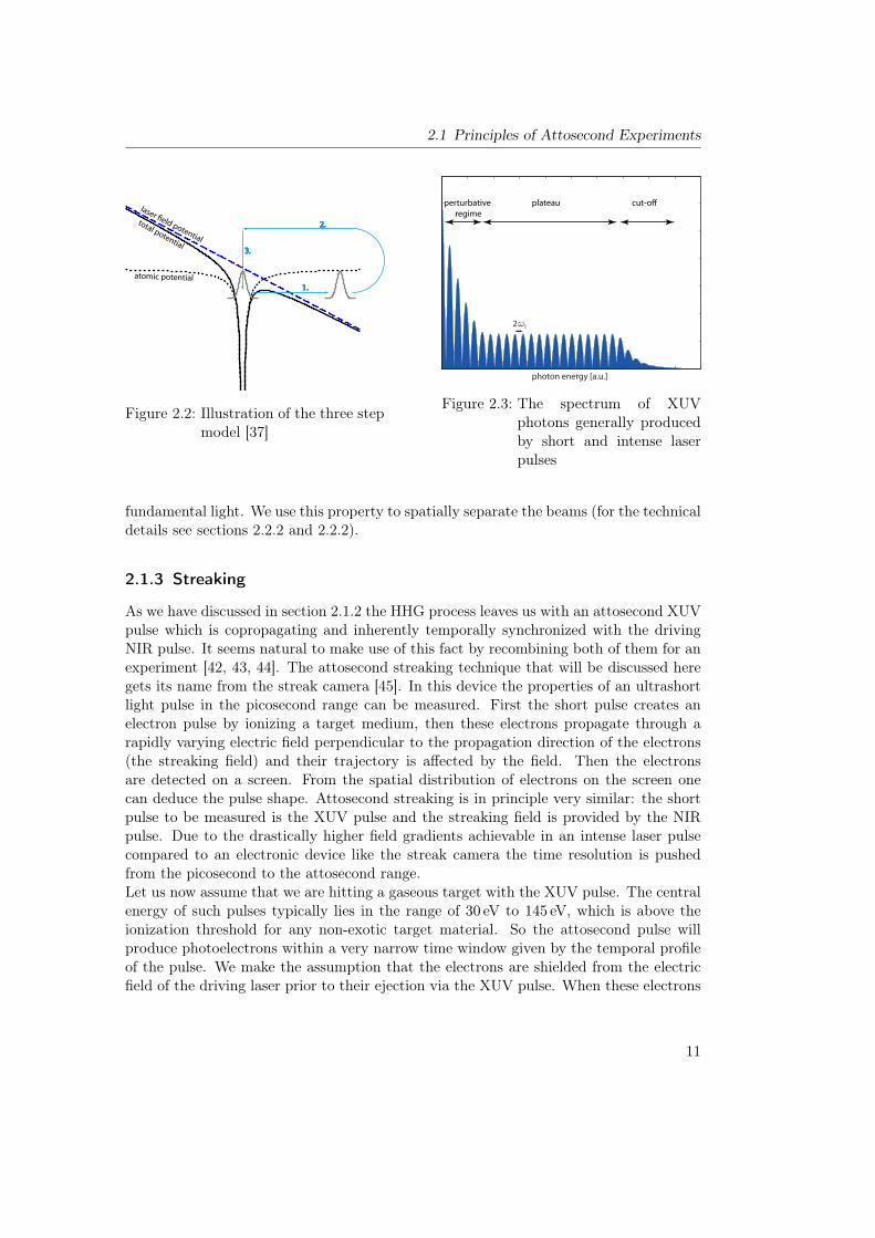
where ✏0 denotes the vacuum permittivity, � is the susceptibility, P (t) is the polarizationvector and EL(t) is the electric field [33]. This approach follows perturbation theory andworks well for low order harmonics (we will follow up on this in chapter 2.1.4). We caneasily see that it predicts the yield for higher harmonics to diminish exponentially withincreasing order (this is the region labeled perturbative regime in figure 2.3). For higherenergies (the plateau region in figure 2.3), the perturbatory approach breaks down. Forvery intense laser pulses2 the harmonics of low orders indeed decrease exponentially, butthe higher orders in the plateau region are produced with almost constant efficiency upto a certain cutoff frequency. This curious behavior can be explained in the semiclassicalthree step model (illustrated in figure 2.2). It describes the process as follows: [11, 34,35]
• The strong electric field bends the potential of the atom, allowing an electron totunnel through the barrier.
• The electron is accelerated away from the ion by the laser field. As the oscillatoryfield reverses direction the electron is accelerated towards the atom and gains energyin the field
• The electron recombines with the atom, shedding its entire gained kinetic energyand the ionization energy in the form of a single high energy photon.
It should be noted that there is also a completely quantum mechanical description ofthis process which was published by Lewenstein et al. in 1994 [36]. It predicts spectrathat are very similar to the semiclassical model and will not be discussed in detail here.Since the HHG process takes half the cycle period of the electric field and it happensduring every half cycle with sufficient field strength we can see from the Fourier transformthat the emitted harmonics are 2!L apart in frequency, where !L denotes the centralfrequency of the driving laser. The typical nonlinear medium in our experiments is neon.It is an inversion symmetric medium and thus we only observe odd harmonics, since theeven terms must vanish. The maximum energy of the plateau region is the cutoff energyEcut-off, which is given by
Ecut-off = Ip + 3.17Up
Up =e2E2
L
4m!2L
,(2.6)
2Intense in this context means that the averaged energy over one field cycle, the ponderomotive energy,is larger than the ionization potential.
9

Chapter 2 Experimental and Theoretical Tools
where e and m are the charge and the mass of the electron, respectively. The factorof 3.17 is the result of the semiclassical calculations in [11]. Up is the ponderomotivepotential and EL is the electric laser field at its peak. Above this energy, the efficiencyof the HHG process decreases exponentially with photon energy. The energy of thereleased photon depends on the exact ionization time and on the path it travels. Thereis an optimum for this time of birth and path for which the highest photon energies arereached [37].Now suppose that we have a driving pulse like the one shown in 2.1b with �CE = 0.It is so short that there is an appreciable difference between the highest spike in theoscillatory field and the next highest one. Here the electrons which are being acceleratedduring the half cycle with the highest field strength will gather the most kinetic energy.They will lead to the release of the highest energy photons in the pulse. This is theprocess responsible for the emission in the cutoff. It is in principle simple to distinguishbetween the plateau and the cutoff regions in a measured spectrum since the cutoff regionshows a much weaker modulation in the photon spectrum than the plateau (as shownin figure 2.3). The origin of the modulation is interference between photons producedduring neighboring half-cycles – but since there is only one half cycle contributing toemission in the cutoff the modulation vanishes. A shorter driving pulse creates a broadercutoff as the range of energy that is only accessible to a single cycle of the field increases.Figure 2.3 shows a mock-up of a typical HHG spectrum. If we now use a combinationof mirrors and filters that transmits only photons from the cutoff region we are left withan isolated pulse of attosecond duration3.Typically we employ a multilayer XUV mirror in the range of 90 eV to 145 eV with abandwidth of 3 eV to 5 eV to focus the XUV light onto the sample [40, 41]. These opticsprovide a gauss shaped reflectivity at the target wavelength. Since the XUV spectralintensity decreases exponentially towards higher photon energies there is a lot more lightat lower energies. Even if the mirror suppresses low energy photons they can still causea stronger signal than the isolated pulse we are interested in. We put a metal filter witha transmission curve that opens up towards the higher energies that we are using in thebeam. In this way we can suppress the unwanted photons at low XUV energies4 in theXUV beam. The metal also suppresses the NIR driving pulse, which is of importance forthe streaking experiments shown in chapter 5.The emitted XUV light copropagates with the fundamental field due to phase matchingin the medium. After careful alignment the two beams are concentric and the XUVmode shape is spherical. The mode shape is extremely sensitive to wavefront curvature.An analysis of the focus with a high resolution camera is not precise enough to makepredictions about it5. The XUV mode is considerably smaller than the mode of the
3This is the most direct approach towards isolated attosecond pulses, but not the only one. Very shortpulses have also been produced with other techniques like polarization gating [38] or relativisticallyoscillating mirror harmonics [39]
4Depending on the photon energy we use zirconium or palladium foils of 150 nm to 200 nm thickness.5Common causes for the introduction of wavefront distortions are imperfectly glued vacuum windows
or mirrors that are fastened too hard. By tightening the nylon tipped screws (never use pure steelscrews) only very, very slightly this can be avoided.
10
2.1 Principles of Attosecond Experiments
1.
2.
3.
laser !eld potential
atomic potential
total potential
Figure 2.2: Illustration of the three stepmodel [37]
plateau cut-o!
photon energy [a.u.]
perturbative regime
2wl
Figure 2.3: The spectrum of XUVphotons generally producedby short and intense laserpulses
fundamental light. We use this property to spatially separate the beams (for the technicaldetails see sections 2.2.2 and 2.2.2).
2.1.3 Streaking
As we have discussed in section 2.1.2 the HHG process leaves us with an attosecond XUVpulse which is copropagating and inherently temporally synchronized with the drivingNIR pulse. It seems natural to make use of this fact by recombining both of them for anexperiment [42, 43, 44]. The attosecond streaking technique that will be discussed heregets its name from the streak camera [45]. In this device the properties of an ultrashortlight pulse in the picosecond range can be measured. First the short pulse creates anelectron pulse by ionizing a target medium, then these electrons propagate through arapidly varying electric field perpendicular to the propagation direction of the electrons(the streaking field) and their trajectory is affected by the field. Then the electronsare detected on a screen. From the spatial distribution of electrons on the screen onecan deduce the pulse shape. Attosecond streaking is in principle very similar: the shortpulse to be measured is the XUV pulse and the streaking field is provided by the NIRpulse. Due to the drastically higher field gradients achievable in an intense laser pulsecompared to an electronic device like the streak camera the time resolution is pushedfrom the picosecond to the attosecond range.Let us now assume that we are hitting a gaseous target with the XUV pulse. The centralenergy of such pulses typically lies in the range of 30 eV to 145 eV, which is above theionization threshold for any non-exotic target material. So the attosecond pulse willproduce photoelectrons within a very narrow time window given by the temporal profileof the pulse. We make the assumption that the electrons are shielded from the electricfield of the driving laser prior to their ejection via the XUV pulse. When these electrons
11
Chapter 2 Experimental and Theoretical Tools
a) b) c)
Δpstreak
pola
rizat
ion
Δpstreak
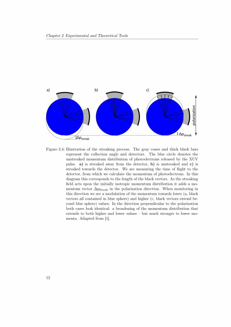
Figure 2.4: Illustration of the streaking process. The gray cones and thick black barsrepresent the collection angle and detectors. The blue circle denotes theunstreaked momentum distribution of photoelectrons released by the XUVpulse. a) is streaked away from the detector, b) is unstreaked and c) isstreaked towards the detector. We are measuring the time of flight to thedetector, from which we calculate the momentum of photoelectrons. In thisdiagram this corresponds to the length of the black vectors. As the streakingfield acts upon the initially isotropic momentum distribution it adds a mo-mentum vector �pStreak in the polarization direction. When monitoring inthis direction we see a modulation of the momentum towards lower (a, blackvectors all contained in blue sphere) and higher (c, black vectors extend be-yond blue sphere) values. In the direction perpendicular to the polarizationboth cases look identical: a broadening of the momentum distribution thatextends to both higher and lower values – but much stronger to lower mo-menta. Adapted from [1].
12
2.1 Principles of Attosecond Experiments
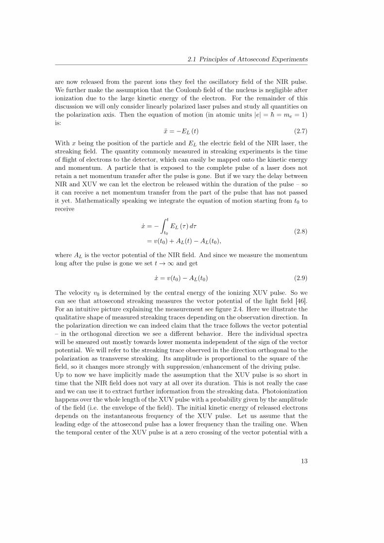
are now released from the parent ions they feel the oscillatory field of the NIR pulse.We further make the assumption that the Coulomb field of the nucleus is negligible afterionization due to the large kinetic energy of the electron. For the remainder of thisdiscussion we will only consider linearly polarized laser pulses and study all quantities onthe polarization axis. Then the equation of motion (in atomic units |e| = h = me = 1)is:
x = �EL (t) (2.7)
With x being the position of the particle and EL the electric field of the NIR laser, thestreaking field. The quantity commonly measured in streaking experiments is the timeof flight of electrons to the detector, which can easily be mapped onto the kinetic energyand momentum. A particle that is exposed to the complete pulse of a laser does notretain a net momentum transfer after the pulse is gone. But if we vary the delay betweenNIR and XUV we can let the electron be released within the duration of the pulse – soit can receive a net momentum transfer from the part of the pulse that has not passedit yet. Mathematically speaking we integrate the equation of motion starting from t0 toreceive
x = �Z t
t0
EL (⌧) d⌧
= v(t0) +AL(t)�AL(t0),
(2.8)
where AL is the vector potential of the NIR field. And since we measure the momentumlong after the pulse is gone we set t ! 1 and get
x = v(t0)�AL(t0) (2.9)
The velocity v0 is determined by the central energy of the ionizing XUV pulse. So wecan see that attosecond streaking measures the vector potential of the light field [46].For an intuitive picture explaining the measurement see figure 2.4. Here we illustrate thequalitative shape of measured streaking traces depending on the observation direction. Inthe polarization direction we can indeed claim that the trace follows the vector potential– in the orthogonal direction we see a different behavior. Here the individual spectrawill be smeared out mostly towards lower momenta independent of the sign of the vectorpotential. We will refer to the streaking trace observed in the direction orthogonal to thepolarization as transverse streaking. Its amplitude is proportional to the square of thefield, so it changes more strongly with suppression/enhancement of the driving pulse.Up to now we have implicitly made the assumption that the XUV pulse is so short intime that the NIR field does not vary at all over its duration. This is not really the caseand we can use it to extract further information from the streaking data. Photoionizationhappens over the whole length of the XUV pulse with a probability given by the amplitudeof the field (i.e. the envelope of the field). The initial kinetic energy of released electronsdepends on the instantaneous frequency of the XUV pulse. Let us assume that theleading edge of the attosecond pulse has a lower frequency than the trailing one. Whenthe temporal center of the XUV pulse is at a zero crossing of the vector potential with a
13

Chapter 2 Experimental and Theoretical Tools
rising slope we can observe the following behaviour: the leading photoelectrons of lowerkinetic energy would be accelerated while the trailing photoelectrons of higher kineticenergy would be decelerated. In total this would make the spectrum narrower. Onthe falling slope of the vector potential we would be able to observe the opposite: abroadening of the spectrum [47].While a full derivation of the retrieval of XUV and NIR pulses will not be discussed hereit shall be mentioned that this technique does not only measure the temporal evolutionof the two pulses that interact with the electrons – the retrieved spectra also carry asignature of the transition matrix element from the medium to the free state and onecould potentially use that to learn something about these matrix elements [48].There are two typically used algorithms for the extraction of delay times from streakingspectrograms: the Center Of Energy (COE) method [20] and the approach relying onsolving the Time Dependent Schrödinger Equation (TDSE). The algorithm for the COEmethod applies the following steps:
• subtract the background
• find the center of energy of the photoline for each delay step (either by a firstmoment analysis or a Gaussian fit to the spectrum)
• fit a streaking waveform of she shape
S(⌧) = S0e�4ln2((⌧+�⌧)/⌧L)2sin(!L(⌧ +�⌧) + �CE) (2.10)
to the data.
Here S0,⌧L and !L denote the streaking amplitude, pulse length and frequency of theNIR streaking laser respectively, �CE is the carrier envelope phase. The parameter �⌧is used when there is more than one photoline present, as will be discussed in chapter5. This method yields no information about the temporal properties of the XUV pulse.The TDSE algorithm is more complex and reveals more physical parameters from thespectrogram. This calculation makes the assumption that the physics of XUV photoion-ization are well represented through the single active electron picture and first orderperturbation theory. It also requires the transition dipole matrix elements to remainconstant over the range of the experiment. This is the case when studying photoioniza-tion far away from resonances and with small relative bandwidths. For the modeling ofthe interaction with the laser field it is assumed that the final state kinetic energy of thephotoelectron is much greater than the ionization potential of the neutral atom. Basedon these prerequisites a transition matrix element is constructed that depends on theparameters of the NIR and XUV pulse. A first guess for the input values is made basedon known attributes of the system such as the XUV mirror bandwidth or the NIR pulselength and central wavelength. Then the parameters are varied by a MATLAB programin order to find the best fit to the spectrogram. A more detailed description can be foundin the Master’s thesis of Ossiander [49], who wrote the retrieval software employed forthe streaking experiments performed in this thesis.
14

2.1 Principles of Attosecond Experiments
2.1.4 Generation of Ultrashort UV Pulses
For now our toolbox contains intense and phaselocked near infrared pulses and very shortXUV pulses. Now we will add another part of the spectrum: deep UV pulses.We are again creating photons of higher energy from our NIR driving pulses. As we cansee from equation 2.5 the polarization response of a medium to intense light pulses willcontain terms that are proportional to the square, cube. . . of the impinging electric field.If we write the time dependent part of the field in the complex representation E(t) / ei!t
we immediately see that this corresponds to terms with twice, three times. . . the frequencyappearing
P =✏0
⇣�(1)EL(t) + �(2)EL(t)
2 + �(3)EL(t)3 + . . .
⌘
=✏0
⇣�(1)ei!t + �(2)ei2!t + �(3)ei3!t + . . .
⌘.
(2.11)
This is of course a simplification of the involved processes. There are many other phe-nomena that are associated with nonlinear optics that will not be mentioned here. Forreference, see [33].Within the perturbative regime the conversion efficiency for a second order process ismuch higher than for a higher order process. So one might be tempted to suggest secondharmonic generation (SHG) as a means for ulstrashort pulse generation in the deep UV.There have indeed been very successful attempts at this endeavor, creating sub 10 fspulses [50, 51]. But the very shortest pulses below 3 fs have been achieved with thirdharmonic generation (THG) [52]. The technical reason for this is that second harmonicgeneration is not possible in a gas. If we consider a medium with complete inversionsymmetry, the even terms of the expansion must vanish for symmetry reasons. So forSHG we need a medium without inversion symmetry – a carefully selected solid. But inthe UV range dispersion is much stronger than in the visible and increasingly harder tocombat for shorter and shorter pulses. In addition the intensities that we would likelybe using are above the damage threshold for most solids. So we are avoiding strongdispersion and damages by using a suitable medium: a gas, in our case neon.In our case frequency tripling has another benefit: the central wavelength of our pulsestranslates to a third harmonic centered at 265 nm, which overlaps with the absorptionbands of DNA and ozone, two very important compounds that could possibly be studiedwith our setup.
2.1.5 Measurement of Femtosecond Pulses: FROG
One of the biggest appeals of ultrafast science is also one of its standard problems: there isno measurement device in the laboratory that rivals the time resolution of the employedpulses. To characterize the pulses one typically has to use a replica of the pulse as agating mechanism. This replica is delayed by ⌧ and overlapped with the original in anonlinear medium, which yields a spectrogram of the form:
S(!, ⌧) =
����Z 1
�1E(t)g(t� ⌧)e�i!tdt
����2
, (2.12)
15
Chapter 2 Experimental and Theoretical Tools
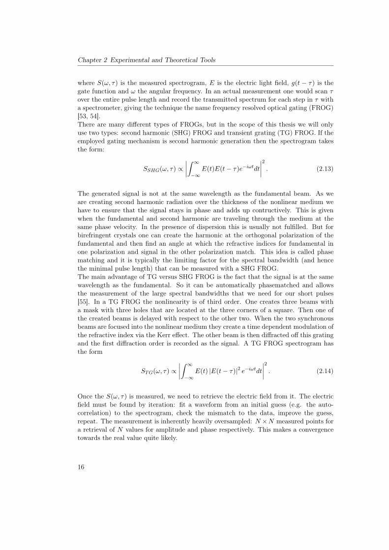
where S(!, ⌧) is the measured spectrogram, E is the electric light field, g(t � ⌧) is thegate function and ! the angular frequency. In an actual measurement one would scan ⌧over the entire pulse length and record the transmitted spectrum for each step in ⌧ witha spectrometer, giving the technique the name frequency resolved optical gating (FROG)[53, 54].There are many different types of FROGs, but in the scope of this thesis we will onlyuse two types: second harmonic (SHG) FROG and transient grating (TG) FROG. If theemployed gating mechanism is second harmonic generation then the spectrogram takesthe form:
SSHG(!, ⌧) /����Z 1
�1E(t)E(t� ⌧)e�i!tdt
����2
. (2.13)
The generated signal is not at the same wavelength as the fundamental beam. As weare creating second harmonic radiation over the thickness of the nonlinear medium wehave to ensure that the signal stays in phase and adds up contructively. This is givenwhen the fundamental and second harmonic are traveling through the medium at thesame phase velocity. In the presence of dispersion this is usually not fulfilled. But forbirefringent crystals one can create the harmonic at the orthogonal polarization of thefundamental and then find an angle at which the refractive indices for fundamental inone polarization and signal in the other polarization match. This idea is called phasematching and it is typically the limiting factor for the spectral bandwidth (and hencethe minimal pulse length) that can be measured with a SHG FROG.The main advantage of TG versus SHG FROG is the fact that the signal is at the samewavelength as the fundamental. So it can be automatically phasematched and allowsthe measurement of the large spectral bandwidths that we need for our short pulses[55]. In a TG FROG the nonlinearity is of third order. One creates three beams witha mask with three holes that are located at the three corners of a square. Then one ofthe created beams is delayed with respect to the other two. When the two synchronousbeams are focused into the nonlinear medium they create a time dependent modulation ofthe refractive index via the Kerr effect. The other beam is then diffracted off this gratingand the first diffraction order is recorded as the signal. A TG FROG spectrogram hasthe form
STG(!, ⌧) /����Z 1
�1E(t) |E(t� ⌧)|2 e�i!tdt
����2
. (2.14)
Once the S(!, ⌧) is measured, we need to retrieve the electric field from it. The electricfield must be found by iteration: fit a waveform from an initial guess (e.g. the auto-correlation) to the spectrogram, check the mismatch to the data, improve the guess,repeat. The measurement is inherently heavily oversampled: N ⇥N measured points fora retrieval of N values for amplitude and phase respectively. This makes a convergencetowards the real value quite likely.
16
2.2 Equipment
2.2 Equipment
2.2.1 The Laser System: FP3
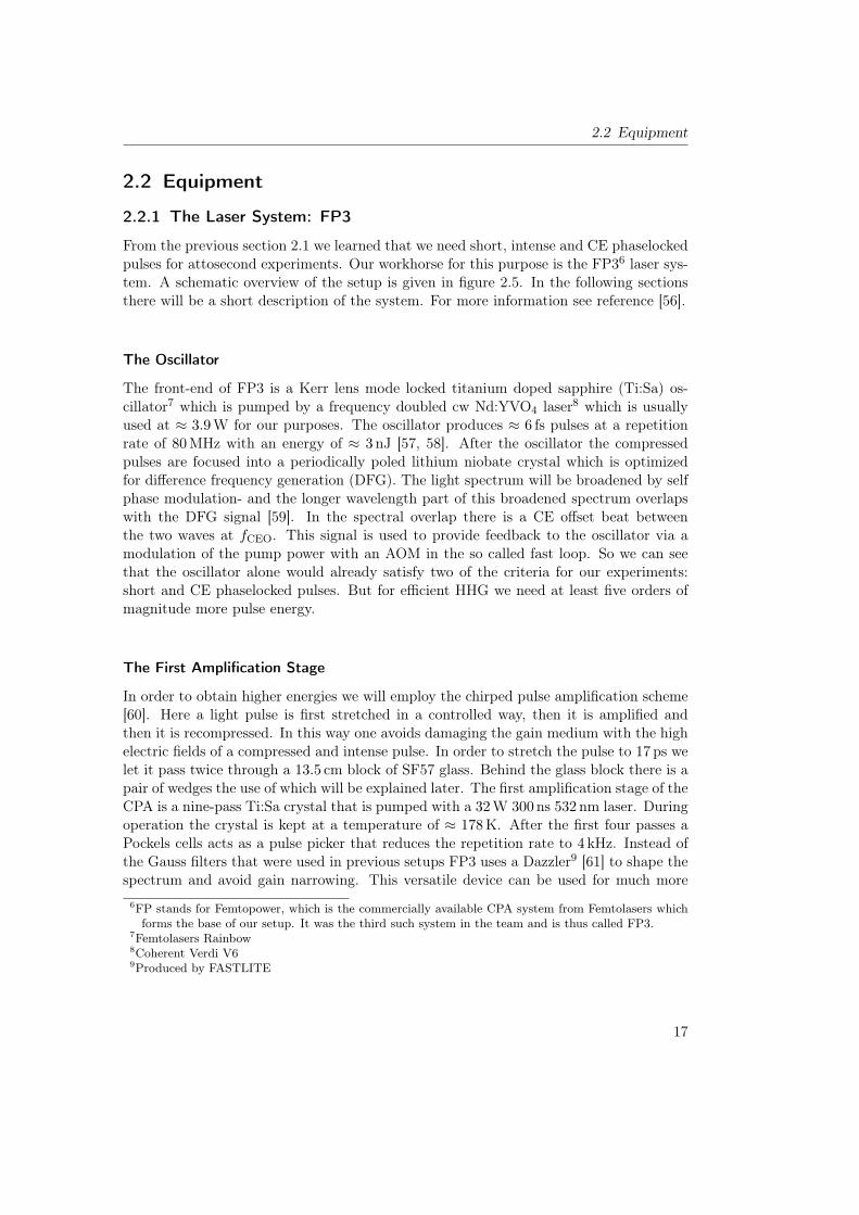
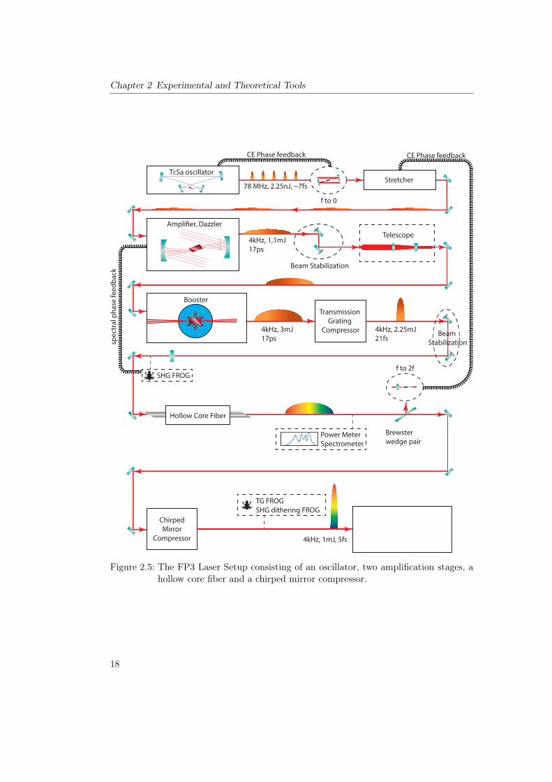
From the previous section 2.1 we learned that we need short, intense and CE phaselockedpulses for attosecond experiments. Our workhorse for this purpose is the FP36 laser sys-tem. A schematic overview of the setup is given in figure 2.5. In the following sectionsthere will be a short description of the system. For more information see reference [56].
The Oscillator
The front-end of FP3 is a Kerr lens mode locked titanium doped sapphire (Ti:Sa) os-cillator7 which is pumped by a frequency doubled cw Nd:YVO4 laser8 which is usuallyused at ⇡ 3.9W for our purposes. The oscillator produces ⇡ 6 fs pulses at a repetitionrate of 80MHz with an energy of ⇡ 3 nJ [57, 58]. After the oscillator the compressedpulses are focused into a periodically poled lithium niobate crystal which is optimizedfor difference frequency generation (DFG). The light spectrum will be broadened by selfphase modulation- and the longer wavelength part of this broadened spectrum overlapswith the DFG signal [59]. In the spectral overlap there is a CE offset beat betweenthe two waves at fCEO. This signal is used to provide feedback to the oscillator via amodulation of the pump power with an AOM in the so called fast loop. So we can seethat the oscillator alone would already satisfy two of the criteria for our experiments:short and CE phaselocked pulses. But for efficient HHG we need at least five orders ofmagnitude more pulse energy.
The First Amplification Stage
In order to obtain higher energies we will employ the chirped pulse amplification scheme[60]. Here a light pulse is first stretched in a controlled way, then it is amplified andthen it is recompressed. In this way one avoids damaging the gain medium with the highelectric fields of a compressed and intense pulse. In order to stretch the pulse to 17 ps welet it pass twice through a 13.5 cm block of SF57 glass. Behind the glass block there is apair of wedges the use of which will be explained later. The first amplification stage of theCPA is a nine-pass Ti:Sa crystal that is pumped with a 32W 300 ns 532 nm laser. Duringoperation the crystal is kept at a temperature of ⇡ 178K. After the first four passes aPockels cells acts as a pulse picker that reduces the repetition rate to 4 kHz. Instead ofthe Gauss filters that were used in previous setups FP3 uses a Dazzler9 [61] to shape thespectrum and avoid gain narrowing. This versatile device can be used for much more
6FP stands for Femtopower, which is the commercially available CPA system from Femtolasers whichforms the base of our setup. It was the third such system in the team and is thus called FP3.
7Femtolasers Rainbow8Coherent Verdi V69Produced by FASTLITE
17
Chapter 2 Experimental and Theoretical Tools
Transmission Grating
Compressor
Transmission Grating
Compressor
Ti:Sa oscillator
78 MHz, 2.25nJ, ~7fs
f to 0
Beam Stabilization
TelescopeAmpli!er, Dazzler
4kHz, 1,1mJ17ps
Booster
4kHz, 3mJ17ps
4kHz, 2.25mJ21fs
Hollow Core Fiber
Beam Stabilization
f to 2fSHG FROG
TG FROGSHG dithering FROG
ChirpedMirror
Compressor 4kHz, 1mJ, 5fs
Stretcher
CE Phase feedback CE Phase feedback
spec
tral
pha
se fe
edba
ck
Brewster wedge pair
Power MeterSpectrometer500 600 700 800 900 1000
0
0.1
0.2
0.3
0.4
0.5
0.6
0.7
0.8
0.9
1
wavelength [nm]
Inte
nsity
[a.u
.]
Figure 2.5: The FP3 Laser Setup consisting of an oscillator, two amplification stages, ahollow core fiber and a chirped mirror compressor.
18

2.2 Equipment
than just static filtering of the spectrum. It is capable of changing the spectral phaseand even the CE phase. This allows one to fine tune the compression the output pulseof the CPA in a simple manner which will be discussed in more detail below. It alsomakes it possible to alternate the CE phase by a desired value (usually ⇡) between twoadjacent pulses. It will become apparent in section 4 why doing this can be beneficialfor an experiment. Finally, after passing through the crystal for 5 more times the pulseis amplified to 1.05mJ to 1.15mJ. It is not necessary to have this stage running at themaximum possible power as long as one is able to extract the maximum usable powerout of the second amplification stage.
The Booster
The second amplification (Booster) stage is also a Ti:Sa multipass system pumped bytwo mode-locked 532 nm pump lasers10. Apart from the general idea however, it differssignificantly from the first stage in multiple respects. First of all it is only a three passsystem that has a much lower amplification factor. The goal here is not to increase theenergy by orders of magnitude but rather by roughly a factor of three. Secondly thecrystal is cooled to the much lower temperature of 58K. This reduces thermal lensingand thus improves the mode profile since the thermal conductivity of sapphire increaseswith decreasing temperature. Of course it also introduces the technical complicationsassociated with a cryogenically cooled setup. Thirdly the focusing into the crystal isvery loose in order to avoid damages to the crystal. In fact the focusing is so loose thatthe entire setup of the booster is within the Rayleigh range of one of the tree passes.This fact makes refocussing the beam into the crystal challenging. Intuitively one wouldassume that moving the focusing optic would also move the focus. But if the optic isplaced within the Rayleigh range of the beam the position of a focusing optic changesalmost nothing about the focus. Only the curvature of the optic has a significant impact.But unfortunately it is necessary to set two parameters when adjusting the focus: wehave to match the focus size of the seed beam to the pump beam and we have to set thefocus position inside the crystal. The solution to this conundrum is a telescope before thebooster with which ce can precisely set the beam diameter and divergence. The correctcombination of refocusing optics for each respective pass inside the booster with thecorrect seed beam parameters can only be found when running the system at full powerbecause the thermal lens changes the divergence markedly. Despite these considerabledifficulties during alignment the system is very user friendly once set up. Two positionsensitive diodes that are spaced far apart are used to mark the beam path of the seedpulse. If the incoupling is done carefully in this manner it is possible to run the systemfor months without the need for any alignment of the booster stage. At this stage thepulse power reaches 2.5mJ to 3mJ.
10Thales ETNA HP.
19

Chapter 2 Experimental and Theoretical Tools
!150 !100 !50 0 50 100 150370
380
390
400
410
420
time delay [fs]
wav
elen
gth
[nm
]
0.0
0.2
0.4
0.6
0.8
1.0
!150 !100 !50 0 50 100 150370
380
390
400
410
420
time delay [fs]
wav
elen
gth
[nm
]
700 750 800 850 9000
0.25
0.5
0.75
1
wavelength [nm]
Inte
nsity
[a.u
.]
!3
!1
1
3
5
7
Phas
e [ra
d]
!150 !100 !50 0 50 100 1500
0.25
0.5
0.75
1
time [fs]
Inte
nsity
[a.u
.]
!5
0
5
10
Phas
e [ra
d]
Sign
al st
reng
th [a
.u.]
Figure 2.6: SHG FROG measurement and retrieved pulse in temporal and frequencyspace of the output of the booster after the transmission grating compressor(see figure 2.5). The retrieved pulse length is 21.5 fs, which is essentiallyFourier limited.
20

2.2 Equipment
Recompression and Spectral Phase Feedback
After recollimation the pulse is compressed in a transmission grating compressor with86% transmission efficiency [62]. We are not using the same method for compression asfor stretching and so we can expect not to compensate the higher order chirp. Here thedazzler comes into play again. There is a second harmonic FROG after the compressorthat can be included in the beam path with a glass wedge on a flip mount. The spectralphase that is extracted from a measurement with this device can be subtracted from thepreviously applied phase in the dazzler. This does not necessarily result in a compressedpulse because there could be nonlinear effects on the way to the FROG that would changein addition to the applied phase feedback. But in that case one can simply iterate andrepeat the phase measurement and the feedback cycle until the pulse is sufficiently com-pressed. Typically no more than three such iterations are necessary. A measurement ofsuch a compressed pulse at this stage of the setup can be seen in figure 2.6. It shows theretrieval of a 21.5 fs pulse, which is almost identical with the Fourier limit.
Supercontinuum Generation and Final Compression
In order to obtain a few cycle pulse the spectrum is then broadened in a Neon filledhollow core fiber (HCF). The produced supercontinuum (see figure 2.7) stretches from400 nm to 1100 nm. With harder focusing and a different fiber geometry it is also possibleto broaden the spectrum further, but since the wavelength range that we can compresswith the chirped mirrors on hand11 ranges from 550 nm to 1100 nm the first step towardsshorter pulses would be the extension of the chirped mirror range – not the spectrum. Thebroadened spectrum easily spans an octave and enables f-to-2f CE phase detection [63,64]. The result of this measurement is fed back on a piezo motorized double prism in frontof the amplifier stage for CE phase stabilization. This is the slow loop complementingthe fast loop inside the oscillator.The compression for the higher energy system does not simply follow the same procedureas for the one stage amplifier. Due to the higher pulse energy we see filamentation at theexit of the hollow core fiber, which changes the beam profile and potentially the temporalprofile – especially because it keeps the beam profile very compact as it propagatesthrough the exit window of the fiber tube. There could be nonlinear effects in thiswindow that we cannot easily prevent. In the near future a double sided differentiallypumped fiber will be installed. The much lower gas pressure at in and outlet will preventfilamentation and improve the beam profile.
Measuring the Compressed Supercontinuum:Transient grating and external dithering FROG
To check the compression after supercontinuum generation a TG-FROG is in use. Whilethe trivial phase matching condition of the TG process means that TG-FROG is in prin-11
PC5, for specifications see http://www.ultrafast-innovations.com/index.php/database/article/174-pc5
21

Chapter 2 Experimental and Theoretical Tools
500 600 700 800 900 10000
0.2
0.4
0.6
0.8
1
wavelength [nm]
Inte
nsi
ty [
a.u
.]
before chirped mirrorsafter chirped mirrors
Figure 2.7: Comparison of supercontinuum spectra created at 1.2 bar in the hollow corefiber before and after compression via chirped mirrors. It is evident that thesespecific mirrors cut the blue part of the spectrum up to 850 nm. This reducesthe bandwidth and lengthens the minimally achievable pulse duration.
ciple able to measure extremely broad spectra the strong alignment dependence of themeasurements makes it difficult to use. This diagnostic is not in use everyday and soit is usually necessary to realign it completely once it does get used. There is no directway to judge whether a trace is correctly showing an uncompressed pulse or whether theFROG itself is not well aligned12. A typical measurement yields a pulse duration of 5.5 fsfor optimum compression. The currently achievable pulse duration is not as short as onecould expect, given the sub–4 fs performance of similar one stage amplifier systems [65].But for many experiments, notably the delay measurements performed for this thesis(see section 5) it is absolutely short enough.In a SHG FROG the situation is easier. Not only is it simpler to align in the first place,but also there is one criterion that allows one to judge the alignment of the interferom-eter in one glance: the trace has to be symmetric. Unfortunately the large bandwidthof the supercontinuum makes a SHG measurement difficult. One can either use a thicknonlinear crystal (and lose phasematching bandwidth) or a very thin crystal (and lose alarge part of the signal). A possible solution is provided by the dithering method [66].Here the crystal is swiftly rotated during the acquisition of a single delay step in a FROGmeasurement. This leads to a different central phasematched wavelength for each rota-tion angle. Since the rotation is performed faster than the acquisition the result is anaverage over the entire phasematching range. For a thick crystal with a precisely definedphasematched frequency this amounts to scanning a delta-like function over the spectrumand then adding up all the frequencies (for each delay step). In this manner it is possibleto greatly increase the bandwidth of a thick crystal. For few cycle pulses this remains
12There is an indirect way: put some material of known dispersion in the beam, measure with andwithout this material and then check if the material dispersion is reproduced correctly.
22

2.2 Equipment
challenging – if one decides to use a thick crystal the pulse is changed significantly by themedium. And for a thin crystal it is essential to place the rotation axis inside the crystalwithout shifting it through the focus. Of course the thinner the crystal, the more precisethe rotation axis has to be placed. With our pulse parameters we would have to use a100 µm to 200 µm thin crystal, making the alignment very difficult. This is why we choseto circumvent this dilemma by modifying the angle of the incoming beam with motor-ized mirrors instead of the crystal. With a camera in place of the crystal the alignmentduring the dithering process can be verified and it can be ensured that the focus doesnot shift significantly, then the camera is replaced by a BBO crystal. Of course this onlydelays the precise alignment problem to a later point: coupling into the spectrometer.But this can again be remedied by using scattering elements like a cosine corrector. Firstmeasurements with the External Dithering SHG FROG have been carried out and lookvery promising [67].
Stability
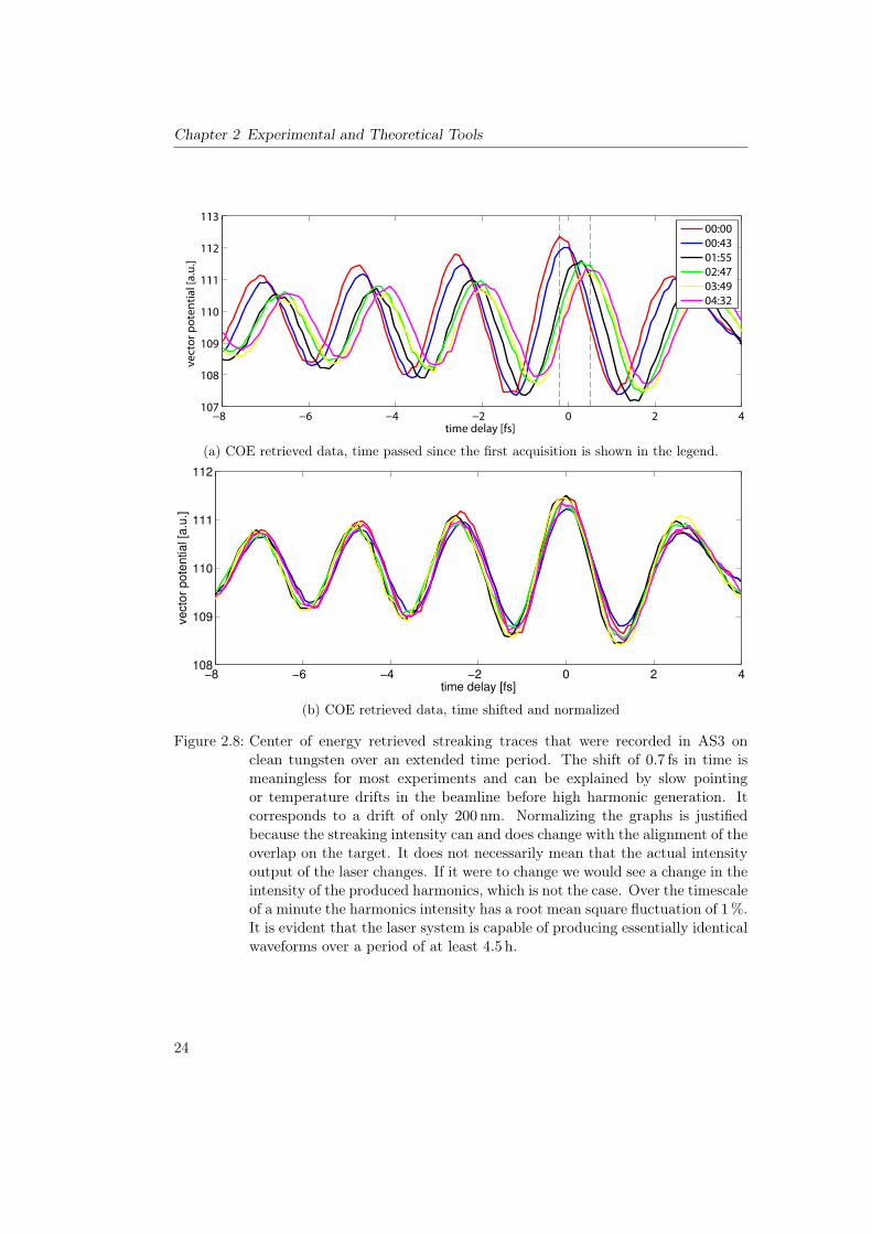
Figure 2.8 shows how stable the laser system is currently running. The traces that areshown here have been recorded in a streaking measurement which has been evaluatedwith the COE method. It is apparent that the laser system produces extremely similarpulses over an extended period of at least 4.5 h. It has to be mentioned that this wasin principle also possible with older systems. The very first streaking measurement in2001 took 8 h [1], which proves that the waveforms were stable at least this long. Butfor these measurements the laser performance was so volatile that experiments were onlypossible at night when the laboratory was quiet. Now we are able to provide a solidlaser performance frequently, even while the lab is busy. The stability shown here is nowactually the routine performance.
2.2.2 The Surface Science Beamline: AS3
When one has succeeded in producing a few femtosecond pulse it must be sent intovacuum quite soon because air dispersion is strong enough to have an impact on thepulse length. So directly after the chirped mirror compressor there is a fused silicaBrewster window that seals an entry port to vacuum. Then the beam is guided to thebeamline of choice. In this thesis two of these setups were used, each with its own uniquecapabilities. The first one we will discuss here is the surface science beamline, AS3 [68].Ultra high vacuum conditions are imperative for performing surface science experimentson many materials. However, for HHG one needs a gas target with pressures on the rangeof 200mbar. So one of the main tasks of the AS3 beamline is to work as a differentialpumping setup that can provide the pressure gradient from 200mbar to 5⇥ 10�11 mbar.An overview of the first vacuum chambers is shown in figure 2.9. The beam enters fromthe right side. It is focused into a quasi static gas cell to produce high harmonics. Theintensity is regulated with an iris diaphragm (A1). Directly behind the HHG targetthere is a skimmer (S, a conical piece of metal with a small hole at the converging side).
23
Chapter 2 Experimental and Theoretical Tools
!8 !6 !4 !2 0 2 4107
108
109
110
111
112
113
time delay [fs]
vect
or p
oten
tial [
a.u.
]
00:0000:4301:5502:4703:4904:32
(a) COE retrieved data, time passed since the first acquisition is shown in the legend.
!8 !6 !4 !2 0 2 4108
109
110
111
112
time delay [fs]
vect
or
pote
ntia
l [a.u
.]
(b) COE retrieved data, time shifted and normalized
Figure 2.8: Center of energy retrieved streaking traces that were recorded in AS3 onclean tungsten over an extended time period. The shift of 0.7 fs in time ismeaningless for most experiments and can be explained by slow pointingor temperature drifts in the beamline before high harmonic generation. Itcorresponds to a drift of only 200 nm. Normalizing the graphs is justifiedbecause the streaking intensity can and does change with the alignment of theoverlap on the target. It does not necessarily mean that the actual intensityoutput of the laser changes. If it were to change we would see a change in theintensity of the produced harmonics, which is not the case. Over the timescaleof a minute the harmonics intensity has a root mean square fluctuation of 1%.It is evident that the laser system is capable of producing essentially identicalwaveforms over a period of at least 4.5 h.
24

2.2 Equipment
-
Y
T
M1
S
L
600LTurbo
200LTurbo
400LTurbo
G
FM
M2
FSP
A2
300LTurbo
A1
X
Z
to the Experiment (p < 10-10 mbar)
HHG Chamber(p >103 mbar)
XUVCCD
Figure 2.9: AS3 beamline (adapted from [69]). S: Skimmer, FM: focusing mirror, FS:filter slider, A1: iris aperture for HHG optimization, A1: iris aperture forstreaking optimization,P:pellicle, G:grating
Over the length of the beamline there are repeated apertures and pumps to reduce thepressure.Behind the experimental chamber (see figure 2.10) there is a multichannel plate (MCP)
combined with a phosphorus screen which is monitored with a CCD camera. With thehelp of appropriate metal filters in the filter slider (FS) it is used to characterize andoptimize the harmonic flux. For further diagnosis the XUV spectrum can be scrutinizedwith a spectrometer (read: a concave grating and a XUV CCD camera) which can beput in the beam path with the help of a movable mirror(M2).In the surface science end station we have access to a number of sample preparation
tools:
• A load lock to keep the main chamber clean when exchanging samples
• A sputter gun for sample cleaning
• A heating and cooling setup with which the sample temperature can be varied from30K to 2400K
• Two types of Knudsen evaporation cells – one for metals (see [22]) and one fororganic molecules13
• A Low Energy Electron Diffraction (LEED) device for structural analysis of surfaces
With a freshly prepared surface we can move the sample over to the experimental chamberand analyze it by performing X-ray Photoelectron Spectroscopy (XPS) [70]. As a lightsource for this technique we have a cw X-ray source with an aluminum cathode at 1486 eVand a magnesium cathode that emits at 1253 eV. The high photon energy makes itpossible to reach a large number of core states that cannot be accessed with our XUVpulses. The typical flux rates are also significantly higher and the energy resolution is13A 4-cell evaporator by Dodecon
25
Chapter 2 Experimental and Theoretical Tools
CCD
MCP
Z X
Y
Load-LockSystem
LEED
Knudsen-Cell
Sputter GunGas Doser
Sample
TOFHEA
2-Component Mirror
X-ray Source
Entry Port
70LTurbo
700L
Turbo
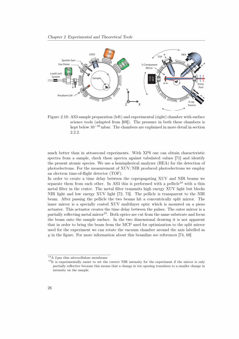
TSP
Figure 2.10: AS3 sample preparation (left) and experimental (right) chamber with surfacescience tools (adapted from [69]). The pressure in both these chambers iskept below 10�10 mbar. The chambers are explained in more detail in section2.2.2.
much better than in attosecond experiments. With XPS one can obtain characteristicspectra from a sample, check these spectra against tabulated values [71] and identifythe present atomic species. We use a hemispherical analyzer (HEA) for the detection ofphotoelectrons. For the measurement of XUV/NIR produced photoelectrons we employan electron time-of-flight detector (TOF).In order to create a time delay between the copropagating XUV and NIR beams weseparate them from each other. In AS3 this is performed with a pellicle14 with a thinmetal filter in the center. The metal filter transmits high energy XUV light but blocksNIR light and low energy XUV light [72, 73]. The pellicle is transparent to the NIRbeam. After passing the pellicle the two beams hit a concentrically split mirror. Theinner mirror is a specially coated XUV multilayer optic which is mounted on a piezoactuator. This actuator creates the time delay between the pulses. The outer mirror is apartially reflecting metal mirror15. Both optics are cut from the same substrate and focusthe beam onto the sample surface. In the two dimensional drawing it is not apparentthat in order to bring the beam from the MCP used for optimization to the split mirrorused for the experiment we can rotate the vacuum chamber around the axis labelled asy in the figure. For more information about this beamline see references [74, 68]
14A 2 µm thin nitrocellulose membrane15It is experimentally easier to set the correct NIR intensity for the experiment if the mirror is only
partially reflective because this means that a change in iris opening translates to a smaller change inintensity on the sample.
26

2.2 Equipment
WCCD
XUVCCD
fromHHG
FW
FW
T
G
MLM
toExp
MA
DS
to pumps
THGPM
PMM1
M2
Figure 2.11: The delay chamber of AS2 (adapted from [76]). PM: perforated mirror, DS:delay stage, THG: third harmonic generation, MA: motorized aperture, FW:filter wheel, MLM: multilayer XUV mirror, XUC CCD: XUV compatibleCCD camera, T: toroidal mirror, W: glass wedge, CCD: UV/NIR CCDcamera
2.2.3 The Interferometric Beamline: AS2
In the previous section we presented a beamline with a highly sophisticated experimentalend station. For the AS2 beamline the unique capabilities lie in a part that is realizedwith just a split mirror in AS3: the delay chamber (see figure 2.11) [75].As in other beamlines we first generate high harmonics with NIR light in a separate
chamber16. Then we need to spatially separate the two beams. Here the role of thepellicle is played by a perforated mirror (PM). The smaller XUV mode will pass throughthe hole in the mirror while a donut shaped NIR beam will be reflected. In the XUVbeam path we find very similar diagnostics to the AS3: an XUV CCD that can eitherbe used for direct observation of the beam profile (fulfilling the role of the MCP) or asa spectrometer. Here we also have the possibility to use different metal filters which canrapidly be switched through the use of filter wheels (FW). The XUV beam is reflectedon a multilayer mirror (MLM) and recombined with the NIR at the second perforatedmirror. They then both get focused by a Nickel coated grazing incidence toroidal mirror
16Not drawn here – it mainly consists of a focusing mirror and a quasi static gas cell
27
Chapter 2 Experimental and Theoretical Tools
IR CCD
UVSpecUVD
XUVCCD
TS1,2
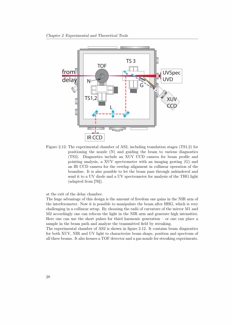
TS 3TOF
NG
L
fromdelay
Figure 2.12: The experimental chamber of AS2, including translation stages (TS1,2) forpositioning the nozzle (N) and guiding the beam to various diagnostics(TS3). Diagnostics include an XUV CCD camera for beam profile andpointing analysis, a XUV spectrometer with an imaging grating (G) andan IR CCD camera for the overlap alignment in collinear operation of thebeamline. It is also possible to let the beam pass through unhindered andsend it to a UV diode and a UV spectrometer for analysis of the THG light(adapted from [76]).
at the exit of the delay chamber.The huge advantage of this design is the amount of freedom one gains in the NIR arm ofthe interferometer. Now it is possible to manipulate the beam after HHG, which is verychallenging in a collinear setup. By choosing the radii of curvature of the mirror M1 andM2 accordingly one can refocus the light in the NIR arm and generate high intensities.Here one can use the short pulses for third harmonic generation – or one can place asample in the beam path and analyze the transmitted field by streaking.The experimental chamber of AS2 is shown in figure 2.12. It contains beam diagnosticsfor both XUV, NIR and UV light to characterize beam shape, position and spectrum ofall three beams. It also houses a TOF detector and a gas nozzle for streaking experiments.
28

Chapter 3
Molecules in the Gas Phase: UV/XUVPump Probe Experiments in Ozone
As outlined in chapter 1 we are exploring the first few femtoseconds of charge rearrange-ment in ozone triggered by intense deep UV light. We argue that the product of thesubsequent molecular decay are determined by the electronic motion driving the nucleardynamics. This is a replica of the photophysics in the stratosphere, where ozone absorbsharmful UV radiation.
3.1 Principle of the Experiment
We perform pump probe photoelectron spectroscopy on pure ozone gas. The sample isexcited via an ultrashort NIR pulse at 1.5 eV or a UV pulse at 4.5 eV. Upon excitation apart of the illuminated molecules will be lifted to the excited state. The valence electronsin this state are less tightly bound than those in the ground state. The molecules will thenbe ionized by an XUV pulse at 130 eV. This releases a photoelectron which we analyzewith our time of flight detector (TOF). From the time of flight and the photon energywe can calculate the kinetic and binding energy of the electrons and distinguish betweenground and excited state. In figure 3.1 the spectra of the fundamental laser beam, thefrequency tripled UV and the absorption spectrum of ozone are shown. Evidently thespectral overlap is especially good in the Hartley band, where the cross section is alsoexceptionally high. Due to the high energy that is available to us in the NIR it seems likepump probe experiments might be possible even with all three pulses combined: NIR,UV and XUV. In this case there could be quantum beats between the populations of theHartley and Chappuis and Wulf: the two excited states are simultaneously and coherentlypopulated – so they can form a wavepacket that evolves in time and the population swapsback and forth between them. We will address the experimental feasibility of this insection 3.4.
3.1.1 Time Resolution versus Energy Resolution: The Choice of XUVMirror
Attosecond photoelectron spectroscopy on molecules faces a fundamental conundrum.In these experiments we would like a high time resolution to track the evolution of thesystem – but we also need an appreciable energy resolution to resolve the signals. And in
29

Chapter 3 UV/XUV Pump Probe Experiments in Ozone
200 300 400 500 600 700 800 900 100010!24
10!22
10!20
10!18
Wavelength[nm]
Abso
rptio
n cr
oss s
ectio
n [c
m!]
200 300 400 500 600 700 800 900 100010!2
10!1
100
Inte
nsity
[a.u
.]
Hartley Huggins Chappuis Wulf
Figure 3.1: The absorption spectrum of ozone (black, referring to scale on left side offigure), the compressed spectrum of the FP3 laser system (red) and the fre-quency tripled spectrum (blue). Both spectra have been normalized individ-ually. The UV pulses spectrally overlap completely with the Hartley band.In the near infrared there is still some overlap with the Chappuis band. ThisUV spectrum was produced at 8 bar backing pressure in the THG target. [77,78, 79]
attosecond photoelectron spectroscopy both of these are chiefly determined by the sameproperty: the bandwidth of the ionizing XUV pulse. For a gauss shaped spectrum thetime bandwidth product is given by
�⌫ ·�⌧ =2 ln 2
⇡, (3.1)
�E ·�⌧ = 1825[eV][as], (3.2)
where the � denotes the full width at half maximum of the frequency ⌫, the energy Eand the time ⌧ respectively. Since we are mainly interested in dynamics triggered by theUV pulse at 4.5 eV and we need to be able to separate ground and excited state spectrallywe chose a mirror with a bandwidth of 3.5 eV. This yields a temporal resolution of 520 asfor a compressed pulse.
3.2 Sample Preparation: Ozone Distillation
When performing experiments with ozone there is always the danger of contaminatingthe sample with oxygen since ozone is metastable and naturally decays into oxygen. Inour case we would not see any dynamics in oxygen since its absorption cross section isnegligible in the spectral range of interest [78]. But we would still produce photoelectronsfrom oxygen, generating a background and making the actual signal harder to detect. Sowe need purified ozone. In order to judge the implications of this fact let us delve intothe research of the 1950s. During this time ozone was studied not for its atmospheric
30

3.2 Sample Preparation: Ozone Distillation
Ozonizer
to experiment
to pump
silica gel
heat exchanger
heating coil
Reservoir
Figure 3.2: The distillation setup for delivery of pure (> 95%) ozone to vacuum. Afterthe ozonizer all pipes are made from stainless steel. The U-shaped pipecontaining silica gel is made out of glass. In front of the pump there is acatalyst (Carulite 200) that turns the ozone to oxygen and thus protects thepump.
properties but because of its considerable oxidation potential and possible use as rocketfuel [80]. Unfortunately it turned out be unusable not for lack of contained chemicalenergy but due to its extreme instability [81]. Ozone explodes violently when triggeredby vibrations, high temperature, sparks, organic contamination or light. It is also highlycorrosive and toxic. Concentrated ozone can only be handled in containers made ofnonreactive materials such as Teflon, stainless steel or silica. The parts of our setup thatcome into contact with purified ozone are built exclusively out of these materials.In order to obtain pure ozone we proceed in the following way (see also figure 3.2):
• produce low concentration of ozone from oxygen in a gas discharge1
• Let O2/O3 mixture at 600mbar flow through a cold trap at �90 �C filled with silicagel beads
• The silica gel passivates the O2 similar to the sawdust that passivates nitroglycerinin dynamite2
• The higher vapor pressure [82, 83] and smaller surface area of O2 compared to O3
make sure that ozone adsorbs to the silica gel while oxygen does not [84]
• Pump the setup down to a few mbar to dispose of remaining gaseous oxygen
• increase the temperature of the glass tube to �25 �C with a heating coil until thepressure in the reservoir reaches 150mbar to 200mbar
This procedure leaves us with concentrated ozone. In order to measure the concentrationwe measure the pressure in the reservoir, shut it off from the rest of the setup and heat
1Commercially available product: Sander Labor– Ozonisator 301.192Explosions of adsorbed O3 can still happen, but they are much less likely
31

Chapter 3 UV/XUV Pump Probe Experiments in Ozone
it up to 130 �C. At any appreciable concentration this leads to an explosion. Accordingto
2O3 ! 3O2 (3.3)
for a formerly pure sample of ozone the pressure would increase by a factor of 1.5 (aftercooling down to the temperature at the start of the procedure). In the presence ofimpurities and the residual pressure of oxygen p0 when pumping down after adsorptionwe see a somewhat smaller pressure increase from ps to pe. Assuming an ideal gas andconstant volume we get the ozone concentration
C(O3) = 2pe � psps � p0
(3.4)
Note that here we are calculating the concentration of ozone in the gas that was desorbedfrom silica gel, not in the total amount of gas. It makes sense to consider this quantitybecause we will be constantly taking gas out of the volume and replenishing it throughdesorption. So the purity of the replenishing gas is the quantity of interest.We typically reach purities of 95% (in the total gas after desorption) and 99% (in thedesorbing gas). After two and a half hours of continuous desorption the concentration isstill 95%, which is sufficient for our experiments3.
3.3 UV Generation and IR Suppression
3.3.1 UV Generation
As we have argued in section 2.1.4 our method of choice for ultrashort pulse generationis frequency tripling in a gas. The high pulse energy that we are using dictates a mediumwith a very high ionization threshold: Neon. Even if Argon or SF6 have higher nonlin-earities strong ionization leads to saturation and limits the maximum yield from thesegases [85]. Since we are forced to use a medium with a low yield per atom we have tomake sure that we have the maximum possible amount of atoms in the beam and usehigh pressures. The quasistatic gas cells that we were using in the beginning are simplystainless steel tubes with two small holes for laser entry and exit and a gas feed line.We predrilled the holes with diameters of 300 µm. But after one to three days of usagethe targets are worn out (see figure 3.3) and damaged by the intense laser. This widensthe holes, prevents pressure buildup inside the target and dramatically decreases the UVyield. It also produces a more painful problem: the ablated material is deposited notonly in the differential pumping chamber but also on the first mirror after the target,which effectively destroys it. Targets made out of aluminum ceramics are a more durablealternative to steel. They are virtually indestructible by our laser4. Target preparationis more difficult since these ceramics are harder than the standard drill bits, but it is still
3The longevity of our ozone did improve over months. We assume that the ongoing passivation of thesetup walls due to ozone exposure is responsible.
4This assumption was experimentally thoroughly tested.
32

3.3 UV Generation and IR Suppression
a1) a2)
a3)
b1) b2)
b3)
300 µm
300 µm
300 µm
300 µm
Figure 3.3: The different types of targets used for UV generation. a) shows the pre-viously prevalent predrilled steel targets. In a2) an unused target is shown,contrasting with a3), a used target. It is apparent that the hole is elliptic andconsiderably widened in the vertical. This would in practice reduce the UVflux. b) shows the ceramics targets with b1) being an unused target and b2)a used one. Also here strong wear is visible, but the central hole is still almostintact. This target was used daily for several weeks. During the alignmentwe were less careful about damaging the target with the full beam than witha steel target and could perform UV flux optimizations significantly faster.
possible. Either one can send the targets to a company that employs CO2 laser drilling5
or one can drill the holes with a high power disc laser available in house [86].While the target is running the Neon flow is substantial. At a backing pressure of 9 bar
we are using 16 000 NLh or 16 %
h of a 50L gas bottle at 200 bar. Keeping in mind that thisgas flow occurs inside the interferometer of the delay chamber we need to take precautionsto keep the mechanical stability of the setup high enough to perform streaking measure-ments. The pump6 for the first differential pumping stage (directly at the gas target, seefigures 2.11, 3.4) is decoupled from the chamber through a helix stabilized pressure hose7.Additionally it is suspended from the laboratory ceiling. The second stage consists ofanother screw pump that is placed far away in a separate room8. While the target is run-ning at 9 bar backing pressure the delay chamber is maintained at 6⇥ 10�3 mbar. Theexperimental chamber is separated from the delay chamber by a plate with an apertureof 4mm. Thanks to this additional barrier the background pressure here is not affectedby the THG target. With this setup we can produce up to 7 µJ of deep UV pulses, whichis also shown in figure 3.5.
5We used LiLa Laser
6A Busch Cobra screw pump7These hoses may look crude in a high vacuum setup, but they provided a supreme vibrational decou-
pling – much better than the membrane bellows previously used for the same purpose.8Leybold Screwline
33

Chapter 3 UV/XUV Pump Probe Experiments in Ozone
to pumps
THG
9 bar Neline
to pumps
540μJ NIR 7μJ UV
50 μm fused silicawindow Silicon chicane
IR suppressingUV mirrors
perforatedbarriers
Figure 3.4: Cutout of the delay chamber of AS2 (figure 2.11). Neon is put into thechamber at up to 11 bar backing pressure. The target is motorized and canbe positioned independent of the surrounding pumping stage. The differentialpumping stages are separated from the main chamber by a 50 µm thin fusedsilica window and two perforated barriers. The IR suppressing mirrors andthe silicon chicane are optional and are discussed in section 3.3.2. The siliconmirrors are used at Brewster’s angle and have to be placed such that theyreflect the beam up- or downwards due to the s-polarized field.
34
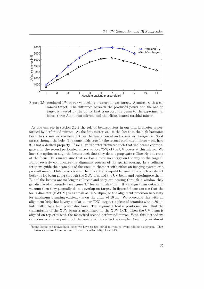
3.3 UV Generation and IR Suppression
1 2 3 4 5 6 7 8 9 10 110
1000
2000
3000
4000
5000
6000
7000
Absolute backing pressure[bar]
UV
pu
lse
en
erg
y [n
J]
Produced UVUV on target
Figure 3.5: produced UV power vs backing pressure in gas target. Acquired with a ce-ramics target. The difference between the produced power and the one ontarget is caused by the optics that transport the beam to the experimentalfocus: three Aluminum mirrors and the Nickel coated toroidal mirror.
As one can see in section 2.2.3 the role of beamsplitters in our interferometer is per-formed by perforated mirrors. At the first mirror we use the fact that the high harmonicbeam has a smaller wavelength than the fundamental and a smaller divergence. So itpasses through the hole. The same holds true for the second perforated mirror – but hereit is not a desired property. If we align the interferometer such that the beams copropa-gate after the second perforated mirror we lose 75% of the UV power at this mirror. Wehave the option to align the beams such that they do not propagate collinearly but crossat the focus. This makes sure that we lose almost no energy on the way to the target9.But it severely complicates the alignment process of the spatial overlap. In a collinearsetup we guide the beam out of the vacuum chamber with either an imaging system or apick–off mirror. Outside of vacuum there is a UV compatible camera on which we detectboth the IR beam going through the XUV arm and the UV beam and superimpose them.But if the beams are no longer collinear and they are passing through a window theyget displaced differently (see figure 3.7 for an illustration). If we align them outside ofvacuum then they generally do not overlap on target. In figure 3.6 one can see that thefocus diameter (FWHM) is as small as 50⇥ 70µm, so the alignment precision necessaryfor maximum pumping efficiency is on the order of 10 µm. We overcome this with analignment help that is very similar to our THG targets: a piece of ceramics with a 80 µmhole drilled by a high power disc laser. The alignment tool is positioned such that thetransmission of the XUV beam is maximized on the XUV CCD. Then the UV beam isaligned on top of it with the motorized second perforated mirror. With this method wecan transfer a large portion of the generated power to the sample. Assuming an almost
9Some losses are unavoidable since we have to use metal mirrors to avoid adding dispersion. Thatforces us to use Aluminum mirrors with a reflectivity of ca. 85%
35

Chapter 3 UV/XUV Pump Probe Experiments in Ozone
50
100
150
53µm
a) c)b)
Figure 3.6: UV Beam profile at the focus in the experimental chamber underneath theTOF detector at different pressures in the THG target (a: 2 bar, b: 5 bar,c: 8 bar). The full width at half maximum (FWHM) of a two dimensionalGaussian with arbitrary rotation fitted to the spot at 8 bar is 50⇥70µm2 andalmost identical at other pressures.
compressed pulse of 3.5 fs FWHM we can reach an intensity of 2.4⇥ 1012 W/cm2 on tar-get.Employing the frequency tripling approach with compressed pulses from a system very
similar to FP3 pulse lengths of 2.8 fs have been demonstrated [52]. In this work there areno compression techniques in use after the tripling process. Since we are using preciselythe same approach as in the work of Reiter et al. we made the assumption that ourpulses would also be compressed and started the experiment without the capacity forUV pulse length measurement. Nevertheless it is noteworthy that a measurement of thepulse length with one of the three following approaches is planned and preparations havebegun. Such a measurement should be possible with:
• A transient grating FROG 2.1.5. Here we need a very thin nonlinear medium sowe change the UV pulse as little as possible during the measurement. A similardevice has successfully been used by Graf and coworkers [85]. A downside tothis approach is the fact that the pulse always has to propagate through somemedium that potentially changes its temporal structure even if it is as little as the10 µm thin fused silica slides available to us. It would be possible to design theFROG such that the beam transmitted through the entire apparatus is picked offbehind the experimental chamber in an additional vacuum chamber. In this way ameasurement is possible without disturbing the setup for the actual experiment.
• A UV/UV autocorrelation similar to the one performed in [52]. Here we would needto make drastic changes to the setup. Mounting an ion detector perpendicularly tothe electron detector would not pose a problem in principle. But it would also benecessary to put a split mirror in the beam path of the UV arm of the delay chamberinterferometer. Splitting the mode in this way even when there is currently no pulselength measurement planned would deteriorate the beam quality and reduce theamount of transmitted power.
• A streaking measurement of the UV light. This approach would yield the most
36
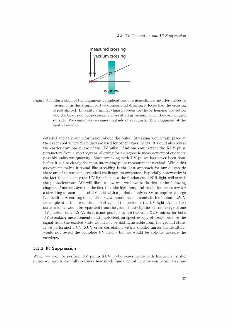
3.3 UV Generation and IR Suppression
vacuum crossingmeasured crossing
window
Figure 3.7: Illustration of the alignment complications of a noncollinear interferometer invacuum. In this simplified two dimensional drawing it looks like the crossingis just shifted. In reality a similar thing happens for the orthogonal projectionand the beams do not necessarily cross at all in vacuum when they are alignedoutside. We cannot use a camera outside of vacuum for fine alignment of thespatial overlap.
detailed and relevant information about the pulse. Streaking would take place atthe exact spot where the pulses are used for other experiments. It would also revealthe carrier envelope phase of the UV pulse. And one can extract the XUV pulseparameters from a spectrogram, allowing for a diagnostic measurement of one morepossibly unknown quantity. Since streaking with UV pulses has never been donebefore it is also clearly the most interesting pulse measurement method. While thisassessment makes it sound like streaking is the best approach for our diagnosticthere are of course some technical challenges to overcome. Especially noteworthy isthe fact that not only the UV light but also the fundamental NIR light will streakthe photoelectrons. We will discuss how well we have to do this in the followingchapter. Another caveat is the fact that the high temporal resolution necessary fora streaking measurement of UV light with a period of only ⇡ 880 as requires a largebandwidth. According to equation 3.2 we would need a bandwidth of about 4.25 eVto sample at a time resolution of 440 as, half the period of the UV light. An excitedstate in ozone would be separated from the ground state by the central energy of oneUV photon: only 4.5 eV. So it is not possible to use the same XUV mirror for bothUV streaking measurements and photoelectron spectroscopy of ozone because thesignal from the excited state would not be distinguishable from the ground state.If we performed a UV/XUV cross correlation with a smaller mirror bandwidth itwould not reveal the complete UV field – but we would be able to measure theenvelope.
3.3.2 IR Suppression
When we want to perform UV pump XUV probe experiments with frequency tripledpulses we have to carefully consider how much fundamental light we can permit to shine
37

Chapter 3 UV/XUV Pump Probe Experiments in Ozone
200 300 400 500 600 700 800 9000
0.2
0.4
0.6
0.8
1
Re!e
ctiv
ity [%
]
200 300 400 500 600 700 800 900
100
150
200
250
300
Phas
e [ra
d]
Wavelength[nm]
Figure 3.8: The reflectivity (black) and phase (green) of the NIR suppressing dielectricUV mirrors. The phase in the NIR has been shifted down by 1150 rad. Thefundamental (red) and THG (blue) spectrum are plotted for comparison withthe reflectance. After two reflections the NIR light is suppressed by roughlytwo orders of magnitude. Also the phase is flat over the majority of theUV spectrum, which means that it does not lengthen the pulse significantly.The reader might wonder why the NIR spectrum differs from the one shownin 3.12 – the spectrum shown here was acquired behind the experimentalchamber with a running HHG and THG target. Especially the THG targetcan be expected to cause spectral shifts in the high pressure gas. The mirrorswere designed and coated by Olga Razskazovskaya.
38

3.3 UV Generation and IR Suppression
on the target without disturbing the experiment. In the experiments with ozone wehave to make sure that we do not change the electronic configuration of the moleculewith the NIR light. One way to find out whether there is an obvious influence of NIRlight on our system is to perform experiments without UV light at high NIR intensities.While this will be discussed in more detail in section 3.5.1 we will forestall the resultand claim that there is no visible change in the photoelectrons due to NIR irradiationapart from streaking. So there are no added requirements for IR suppression to prohibitpopulation in the Chappuis band. If, on the other hand, we wanted to perform a streakingmeasurement of the UV light, the situation is quite different. We need to make sure thatthe UV field will yield the main contribution to the trace. As we can see in equation2.9 the streaking amplitude scales with the vector potential. Calculating the vectorpotential for different wavelengths but identical intensities leaves us with the followingconsideration
A / E0
!
E0 /pI
A /pI
!
) AUV,3! =1
3AIR,!
(3.5)
where A0, E0, I and ! denote the amplitude of the vector potential, the amplitude of theelectric field, the intensity of the field and the frequency of the laser field, respectively. Sosimply the fact that the frequency of our UV field is three times that of the fundamentalcosts us a factor of three in the streaking signal. Adding in the fact that the conversionefficiency from NIR to UV is around 1% we see that we need to suppress the intensity offundamental light by at roughly three orders of magnitude to get a significantly strongersignal from UV streaking than from NIR streaking.Due to the large bandwidth of our UV pulses it is virtually impossible to use optics intransmission in the UV beam path without significantly stretching the pulse in time.This narrows our options down to dichroic mirrors. We have employed two differenttypes of such optics, the first being a specially coated multilayer system that has highreflectivity in the UV and low reflectivity in the NIR (see figure 3.8). In contrast to metalmirrors multilayer mirrors do potentially introduce a considerable spectral phase to thepulse. It is therefore absolutely necessary to have the high reflectivity region extend overthe entire usable spectrum. At the point where the reflectivity drops sharply the phasealso changes rapidly and a reflected pulse would be distorted.While the dielectric mirrors have an even higher reflectivity than metal mirrors theycan potentially stretch a UV pulse. A perfect match between the UV spectrum and thedielectric mirrors has not yet been found, but our efforts are ongoing. An option for NIRsuppression that does not add any spectral phase are silicon mirrors used at Brewster’sangle. This approach has been successfully used in a number of works [87, 52, 85]. Themain idea is simple: while the reflectivity of p-polarized NIR light is very small (in the-ory it is zero) the UV reflectivity is still ⇡ 0.44. In practice it is possible to suppress
39
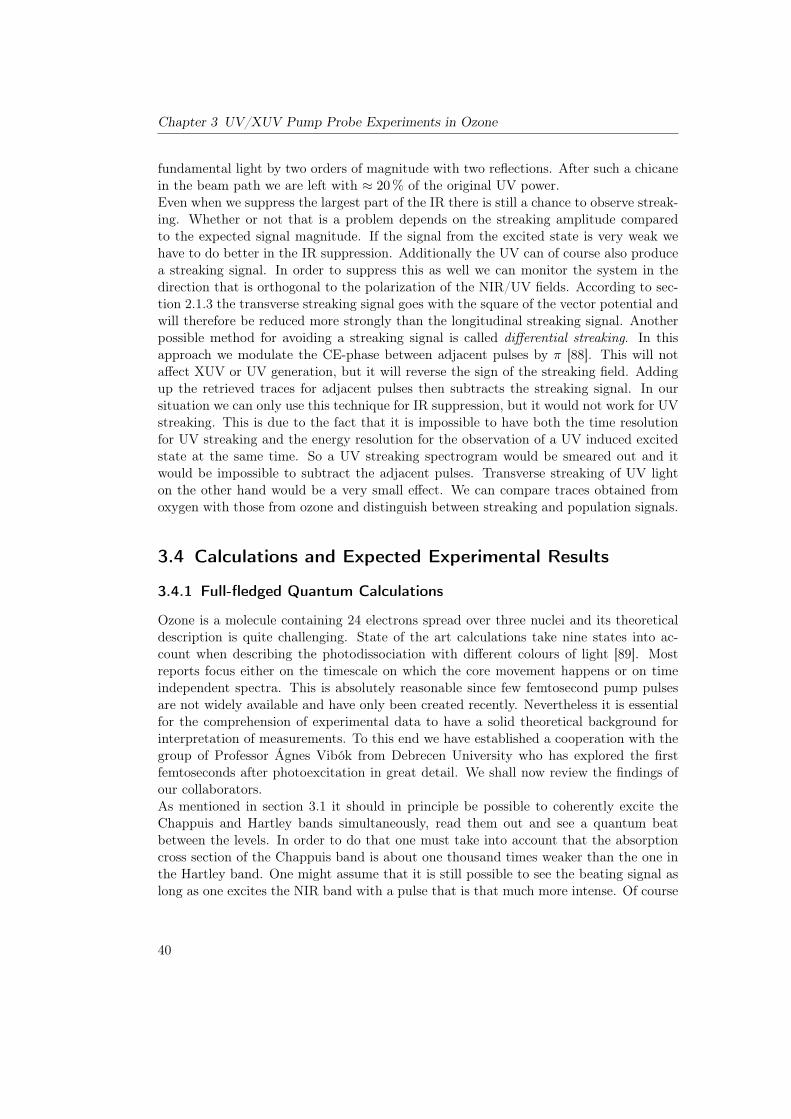
Chapter 3 UV/XUV Pump Probe Experiments in Ozone
fundamental light by two orders of magnitude with two reflections. After such a chicanein the beam path we are left with ⇡ 20% of the original UV power.Even when we suppress the largest part of the IR there is still a chance to observe streak-ing. Whether or not that is a problem depends on the streaking amplitude comparedto the expected signal magnitude. If the signal from the excited state is very weak wehave to do better in the IR suppression. Additionally the UV can of course also producea streaking signal. In order to suppress this as well we can monitor the system in thedirection that is orthogonal to the polarization of the NIR/UV fields. According to sec-tion 2.1.3 the transverse streaking signal goes with the square of the vector potential andwill therefore be reduced more strongly than the longitudinal streaking signal. Anotherpossible method for avoiding a streaking signal is called differential streaking. In thisapproach we modulate the CE-phase between adjacent pulses by ⇡ [88]. This will notaffect XUV or UV generation, but it will reverse the sign of the streaking field. Addingup the retrieved traces for adjacent pulses then subtracts the streaking signal. In oursituation we can only use this technique for IR suppression, but it would not work for UVstreaking. This is due to the fact that it is impossible to have both the time resolutionfor UV streaking and the energy resolution for the observation of a UV induced excitedstate at the same time. So a UV streaking spectrogram would be smeared out and itwould be impossible to subtract the adjacent pulses. Transverse streaking of UV lighton the other hand would be a very small effect. We can compare traces obtained fromoxygen with those from ozone and distinguish between streaking and population signals.
3.4 Calculations and Expected Experimental Results
3.4.1 Full-fledged Quantum Calculations
Ozone is a molecule containing 24 electrons spread over three nuclei and its theoreticaldescription is quite challenging. State of the art calculations take nine states into ac-count when describing the photodissociation with different colours of light [89]. Mostreports focus either on the timescale on which the core movement happens or on timeindependent spectra. This is absolutely reasonable since few femtosecond pump pulsesare not widely available and have only been created recently. Nevertheless it is essentialfor the comprehension of experimental data to have a solid theoretical background forinterpretation of measurements. To this end we have established a cooperation with thegroup of Professor Ágnes Vibók from Debrecen University who has explored the firstfemtoseconds after photoexcitation in great detail. We shall now review the findings ofour collaborators.As mentioned in section 3.1 it should in principle be possible to coherently excite theChappuis and Hartley bands simultaneously, read them out and see a quantum beatbetween the levels. In order to do that one must take into account that the absorptioncross section of the Chappuis band is about one thousand times weaker than the one inthe Hartley band. One might assume that it is still possible to see the beating signal aslong as one excites the NIR band with a pulse that is that much more intense. Of course
40

3.4 Calculations and Expected Experimental Results
this is basically true up to a certain point where the intensity is so high that it triggersunwanted processes such as an excessive amount of ionization. In order to judge thefeasibility of this experiment Halász and coworkers performed the following calculations[27].In a first step the wavefunctions for electrons and cores are separated in the Born–Oppenheimer approximation. Stopping there would of course mean that some of themost interesting and crucial dynamics of the system could not be described. After thefirst 5 fs to 6 fs both electrons and nuclei are in motion. So the electron dynamics areintroduced into the core wavefunctions by means of a nonadiabatic coupling term. Thisterm also includes the electronic coupling to the laser field. Then the time dependentSchrödinger equation including the coupling term is solved in a Multi-Configuration TimeDependent Hartree Fock calculation. The results are used to calculate the density matrixof the system. From the diagonal and off-diagonal elements of the density matrix onecan obtain the populations and coherences of the system. The laser parameters wereclose to what we were expecting to be able to deliver in an experiment, with the addedexception that the UV intensity was adjusted to make sure the populations in both ex-cited states roughly match. This means that the NIR central wavelength was 750 nm at1014 W/cm2 and 4 fs (FWHM). For the UV the parameters were: 260 nm central wave-length at 2⇥ 1011 W/cm2 and 3 fs (FWHM).From these calculations we can learn three main points:
• After 5 fs to 6 fs the cores move and the system is no longer in the Frank Condonregion. Before that the nuclei can be regarded as stationary.
• The symmetry of the ground state and the two excited states in the Hartley andChappuis bands dictates that they cannot be excited with the same polarization.For the effective polarization for UV excitation relative to the molecule, see theinset in figure 3.9b.
• Even at a considerable NIR intensity of 1014 W/cm2 the population in the Chappuisband reaches a mere 1%
Taking the latter two points into account we can conclude that both the simultaneousexcitation and detection of population in both excited states would be extremely chal-lenging. Our UV light is created with the same polarization as the fundamental light.Transmissive optics cannot be used with our short pulses10 and we have no way of ro-tating just one of the two polarizations. Also the population of one percent is usuallybelow the noise level in attosecond photoelectron experiments. In conclusion, the threecolor experiment is probably not feasible. On the bright side, there is no additional re-quirement on the NIR suppression since the effect of fundamental light is so small.After this finding it made sense to study the UV pump/XUV probe setting in more detail[90]. In their next paper Halász et al. used the same approach as before but consideredonly one pump pulse with a central energy of 260 nm and an intensity of 1⇥ 1013 W/cm2
10The combination of the bandwidth, short wavelength of the UV and the large difference in centralenergy of our pulses prohibit the use of waveplates.
41

Chapter 3 UV/XUV Pump Probe Experiments in Ozone
and a pulse length of 3 fs (FWHM). Here the goal was to simulate the largest possiblepopulation and thus the maximum possible UV intensity was taken for the calculation.The main results are:
• At the aforementioned pulse parameters we can transfer about 40% population tothe excited state. As mentioned before it is only possible to excite ozone with onepolarization in the UV. Therefore this result is only valid for aligned molecules.Since we are dealing with a randomly oriented gas we are only populating onethird of the calculated value: 13%. As of now it is not known which cation stateis formed by the ionization from the excited state. This would be necessary fordetermining the polarization response of the system. It is conceivable that theexcited state preferably emits asymmetrically with respect to the polarization axis– and we would have to look for a signal in both directions.
• The Coherence between ground state and excited state rises sharply with the pulse,then decays when the pulse is gone – and rises again to a much smaller value roughly17 fs after the pulse is over (see figure 3.9). The drop in coherence is explaind bythe wavepacket moving away from the Frank-Condon region. For coherence someoverlap between the wavefunctions is necessary. When the overlap is lost, thecoherence is lost as well. The later revival is essentially the reverse process. A partof the wavepacket returns to the Frank-Condon region and can now overlap withthe ground state again. The entire process is much too fast for typical decoherenceprocesses like collisions between gas atoms. Coherence revival in principle is nota new phenomenon and has been seen in experiments at least 30 years ago [91] –obviously not on this ultrashort timescale.
These theoretical predictions have so far concerned only one side of the experiment: thepump process and subsequent dynamics in the system. Now we still need to understandthe probe process and the signal that we could expect. In order to estimate the pho-toelectron spectra Perveaux et al. calculated the Dyson orbitals for Ozone [92]. Theseorbitals are constructed by calculating the overlap of the neutral molecule wavefunctionwith that for the ionized molecule [93]. They have the extremely useful property of beingproportional to the angularly resolved photoelectron yield11. In the next step Perveauxet al. calculated the photoelectron yield for all relevant transitions in a stick spectrum[94]. Then they incorporated the poor spectral resolution of a short XUV probe pulseand convoluted the stick spectrum with a gaussian of FWHM 3.65 eV (see figure 3.10).This corresponds to a time resolution of 500 as. The best way to see the effect of risingpopulation in a photoelectron spectrogram is a differential plot where the ground statespectrum is subtracted from all spectra. Such a spectrum is also shown in figure 3.10.Just as in the previous calculations the pump pulse parameters were: 260 nm centralwavelength, an intensity of 1⇥ 1013 W/cm2 and a pulse length of 3 fs. Here a centralenergy of 95 eV for the probe pulse was used. The key lessons from the calculation basedon Dyson orbitals are:11In our setup we do not have angular resolution, but the photoelectron spectrum can still be reproduced
by integrating over the collection angle or assuming emission along the detector axis.
42

3.4 Calculations and Expected Experimental Results
0.0
0.2
0.4
0.6
0.8
1.0
Popu
latio
n
-4 -2 0 2 4 6 8 10
Time (fs)
Ground stateHartley
(a)
Cohe
renc
e
-10 -5 0 5 10 15 20 25Time (fs)
Coherence between ground state and Hartley
0.0
0.2
0.4
0.6
0.8
1.0
UV polarization
(b)
Figure 3.9: a) Population in ground state and excited state in the Hartley band of ozone.when pumped with intense UV radiation. The 3 fs, 1013 W/cm2 UV pulseused for the calculations is centered at t = 0. b) Coherence between groundstate and Hartley band excited state. The revival at ⇡ 17 fs is clearly visible.The polarization of the UV pump pulse relative to the molecule is depictedin the inset. Note the different scale on the time-axis. Adapted from [90]
0.0
0.1
0.2
0.3
0.4
Rela
tive
inte
nsity
80 85 90Kinetic energy release [eV]
Hartley + Ground State
Ground state
(a)
76
78
80
82
84
86
88
90
92
94
-4 -2 0 2 4 6Time delay [fs]
-0.10
-0.08
-0.06
-0.04
-0.02
+0.00
+0.02
+0.04+0.05
Kine
tic E
nerg
y Re
leas
e [e
V]
(b)
Figure 3.10: a) Calculated photoelectron spectrum of ozone excited with UV pulses at260 nm with an intensity of 1⇥ 1013 W/cm2 and a pulse length of 3 fs. Thisgraph is the result of a stick spectrum of individual transitions that was con-voluted with a Gaussian of FWHM 3.65 eV to take into account the spectralwidth of the XUV pulse centered at 95 eV. The individual absorption linesare represented by dotted lines. b) Differential photoelectron spectrogramsimulating the time evolution of the signal at the Frank-Condon point. Therapid decrease of the differential signal can be attributed to the wavepacketleaving the FC point. Adapted from [94]
43

Chapter 3 UV/XUV Pump Probe Experiments in Ozone
• At the assumed pump parameters of 260 nm central wavelength, 1⇥ 1013 W/cm2
intensity and 3 fs pulse length the differential signal has a contrast of 1.05/0.9 ⇡ 1.17.
• This result is only valid for aligned molecules. The population for non-alignedparticles will be about 1/3 of the population in the aligned case. The contrast for adifferential signal will decrease accordingly.
3.4.2 Three Level Calculations
After reviewing the previous section one might wonder why another type of calculationsis still useful after such a detailed theoretical description. The idea behind it is simple:we needed a way to quickly estimate the experimental outcome when parameters changed– without having to run a supercomputer or having to approach our collaborators. Thesecalculations were performed by Tobias Latka [95]. The Ansatz is a simple Hamiltonianthat shows the three levels and their separation by one UV/NIR photon.
bH0 = h
0
@0 0 00 !NIR 00 0 !UV
1
A (3.6)
With the frequency of the NIR and UV fields denoted by !NIR and !UV. Then thecoupling terms to the field are added in:
bV (t) = �bd · bE(t) = �
0
B@0 ~d01 · ~E ~d02 · ~E
~d10 · ~E 0 ~d12 · ~E~d20 · ~E ~d21 · ~E 0
1
CA (3.7)
~dij = ~d⇤ij (3.8)
Where 0 denotes the ground state, 1 the exited state accessible via a NIR photon, 2the excited state accessible via a UV photon, ~E is the electric field and ~dij is the dipolemoment coupling the states i, j. Then we make the assumption that Electric field anddipole are collinear (as in the more elaborate calculations). Of course this is an Ansatzthat completely neglects nuclear dynamics. But this is justified in the first few femtosec-onds after excitation, which is the time-window we will be concerned with. From here wecalculate the density matrix via the Lindblad formalism [96]. For the magnitude of thedipole moment we can rely on the careful analysis of our collaborators. We perform acalculation for the standard pulse parameters used by Halász et al. and adjust the dipolemoment such that the results match. This results in a dipole moment of 1.85Debye.Then we can change the pulse parameters to those that we see in the experiment. Sincewe already know that the population in the Chappuis band will be near zero we leavethe NIR amplitude at zero and calculate only the Hartley band. An exemplary graph isshown in figure 3.11.When we apply the Ansatz to our parameters we see that we populate approximately
15% of the excited state for aligned molecules- or 5% for non-aligned molecules. Thatwould be about 1/8 of the assumed value for the differential spectrogram in figure 3.10.
44

3.5 Time Resolved Photoelectron Spectroscopy on Ozone
!5 0 5 100
0.2
0.4
0.6
0.8
1
Time [fs]
Popu
latio
n
electric "eld [a.u.]Ground stateHartley
Figure 3.11: The result of a three-level calculation for ozone pumped with UV light withan assumed pulse length of 3.5 fs, a central wavelength of 265 nm and anintensity of 2.4W/cm2. These results can only be trusted for the first fewfemtoseconds because they are obtained while completely neglecting coremovement. They also assume that the molecular dipole moment and electricfield are aligned.
Since we only had a contrast of 1.17 there we can assume to have a weak signal thatrequires a high signal to noise ratio to see the excitation.
3.5 Time Resolved Photoelectron Spectroscopy on Ozone
3.5.1 IR Pump, XUV Probe
From the previous section we learned that an IR induced signal would be very weak andalmost impossible to detect if the data quality is not very good. So the first experimentis the acquisition of a static spectrum in order to judge the attainable signal to noise. Inorder to compare with a well known and easily manageable system we used Neon gas. Forthe results, see figure 3.12. The spectra were acquired under very similar settings rightafter each other (while allowing some time for pumping the Neon gas out of the system).The XUV pulse was centered at 130 eV with a bandwidth of 3.5 eV. Typical acquisitiontimes for a streaking spectrogram with Neon as an electron source range from 1 s to 4 sper individual spectrum. Evidently this is not going to be long enough for experimentswith ozone. We only get acceptable signal to noise ratios for much longer acquisitiontimes from 30 s to 120 s. The reason for this is not only the cross section of ozone andneon but also the slightly different alignment for the beamline when working with UVlight: the high photon energy of the UV light is comparable to the work function of ourmulti channel plate detector. And while it is difficult to see the light reflected off thegas nozzle with NIR light we actually get a huge peak from UV light, because now theelectron generating process is a one photon process as opposed to the three necessaryphotons for NIR. The large light induced peak has an asymmetric tail on the low energyside that can extend all the way to the energy of XUV produced photoelectrons andgenerate a noisy background. To avoid this we have to move the nozzle slightly away
45

Chapter 3 UV/XUV Pump Probe Experiments in Ozone
80 90 100 110 120 130 1400
0.5
1
1.5
2
2.5
x 10 11
Photoelectron Kinetic Energy [eV]
coun
ts [a
.u.]
Ne at 1s intO
3 at 1s int
O3
at 30s int
*0.25
Figure 3.12: Stationary photoelectron spectra of Neon and ozone. The red and blackcurve were obtained at an identical integration time of one second. Theblue spectrum was recorded at 30 s integration (divided by 4 for visibilityof the other spectra). Evidently the signal to noise ratio is much worse forozone at comparable integration times.
from the beam. This strongly reduces the background, but it also reduces the gas densityunder the detector and thus the photoelectron signal. From figure 3.9 we can see thata populated excited state should live for 10 fs without any decline. It seems plausiblethat it would not abruptly cease to exist afterwards but to slowly decay. This is why wechose to perform experiments with few time steps but a long integration time for eachindividual step. Then we can compare the spectra after the pulse to a spectrum beforethe pulse to see first signs of population in the excited state. One such spectrogram isshown in figure 3.13. For this data we increased the NIR intensity so far that the lowerenergy electron background was just outside of our region of interest for XUV producedphotoelectrons. The TOF detector is mounted perpendicularly to the field polarizationto suppress streaking. But we can see that transverse streaking is at least so strongthat it could overwhelm a weak signal from the excited state. So we definitely need tosuppress it for the final experiment.
46
3.6 Conclusions
Delay (fs)
Kin
etic
En
erg
y (e
V)
!5 0 5 10 15 20 25 30
100
105
110
115
120
125
130
0
0.2
0.4
0.6
0.8
1
Figure 3.13: Normalized differential spectrogram of ozone pumped with IR acquired per-pendicular to the IR polarization. The dotted line shows the edge of theground state. Indeed there is a signal above the line. At the same timestepsone can observe a shift of the center of the photoelectron line to smallerkinetic energies. This is transverse streaking as introduced in section 2.1.3.The integration time for this spectrogram was one minute per time step. Anegative time means that the probe pulse comes before the pump pulse.
3.5.2 UV Pump, XUV Probe
Since we now know that sufficiently populating the Chappuis band is next to impossiblewith our experimental setup we study the Hartley band. We learned that we have tosuppress the NIR field to eliminate transverse streaking. At this stage of the experimentthe multilayer mirrors are not usable because we cannot measure the UV pulse durationyet and are there remains considerable uncertainty about the effect of the mirrors onit. So we have to resort to Brewster reflections off of Silicon wafers. This leads to asignificantly reduced UV intensity of about 0.5⇥ 1012 W/cm2. We would not expect tosee a signal at such a low intensity. Figure 3.14 shows a differential spectrogram thatunfortunately confirms our expectations.
3.6 Conclusions
We have designed and built a setup that is capable of creating ultrashort pulses inthe deep UV at a central wavelength 265 nm with pulse energies of up to 7 µJ utilizingfrequency tripling. This setup utilized neon gas at backing pressures from 1 bar to 11 bar,while a differential pumping setup ensures that the gas flow does not affect the adjacenthigh vacuum part of the beamline. While the UV target is running and large amounts ofneon gas are being pumped through the setup we ensured that the mechanical stabilitywas sufficient for streaking experiments. These capabilities were combined with theinterferometric beamline AS2 and now experiments with intense ultrashort deep UV
47

Chapter 3 UV/XUV Pump Probe Experiments in Ozone
Delay (fs)
Kin
etic
Energ
y (e
V)
!10 0 10 20 30 40 50
100
105
110
115
120
125
130
!0.2
!0.1
0
0.1
0.2
0.3
Figure 3.14: Normalized differential spectrogram of ozone pumped with0.5⇥ 1012 W/cm2. There is no discernible signal present.
UV arm
XUV arm
o!-axis parabolic mirrortoroidal mirror
Figure 3.15: The proposed new focusing scheme that would focus the two beams withdifferent optics.
pulses and attosecond XUV pulses are possible.We have created an ozone source that is capable of fueling a gas target for photoelectronexperiments with high purity (⇡ 95%) ozone for at least 2.5 hours.We established a collaboration with the group of Professor Vibók. From their calculationswe learned that the population that we can introduce to the Chappuis band will probablynot be detectable with our setup. We also saw the precise way in which the Hartleyband would be populated and the subsequent dynamics that we can expect. From thiswe learned to judge the UV intensity necessary for a strong enough population in theexcited state to be visible in an experiment. For our current experimental situation asignal can not be expected. In the next section we sketch our next steps to obtain adetectable signal.
48

3.7 Outlook
3.7 Outlook
The experimental difficulty of seeing a signal from the excited state can be viewed fromtwo perspectives: either there needs to be enough population to detect it even with badsignal to noise ratio or we need to change the readout and detection in order to improvethe signal to noise ration and the contrast between ground and excited state.Building on the theoretical results we can assume that we need an order of magnitudehigher UV fields in order to generate a large signal that is easy to detect. It is essentiallyimpossible to generate that much more pulse energy with the gas harmonics that we areusing. But we do not necessarily need higher energies- just higher energy densities ofthe UV light in the volume probed by XUV pulses. Naturally the idea of tighter focus-ing comes to mind. While this is a trivial task for visible wavelengths it can be ratherdemanding for XUV light. We would essentially need a toroidal mirror with a muchshorter focal length. Optics need a surface quality that scales with the wavelength of thereflected light and thus it is very difficult and expensive to obtain large XUV capableoptics. In addition toroidal mirrors are notoriously hard to align – and this behaviourscales unfavorably with decreasing focusing length. So our approach is slightly different:we still focus the XUV light with the toroidal that we are using at the moment. Butwe focus the UV light with a perforated off-axis paraboloid (see figure 3.15). Since theparabolic mirror is placed in the converging part of the XUV beam, the hole in it can besmall. So we would not lose as much energy as before when we are working in a collineargeometry. Tighter focusing would also improve the signal to noise ratio as a smaller UVfocus would permit us to move the gas nozzle closer to the XUV beam, yielding a highergas density at the focus. A smaller focus for only the UV light would unfortunately pro-hibit streaking measurements, for which one needs a homogeneous streaking field overthe XUV focus diameter. As long as both pulses are focused with the same optics thisis certified by the much smaller wavelength of XUV.Another easily implementable way to increase the contrast is by decreasing the spectraloverlap between ground and excited state. An XUV mirror with a smaller spectral band-width would make the separation of the two peaks a lot easier. It would of course havea worse temporal resolution and is not suitable for high end experiments. But even aweak signal can be optimized. A narrow band mirror would certainly help in finding it,optimizing it and then switching mirrors and performing the experiment.As we cannot be sure about the preferred emission direction of photoelectrons from theexcited state it is possible that we have to rotate the NIR polarization relative to theXUV polarization in order to fulfill two criteria simultaneously: electron detection inthe transverse streaking direction and in the main photoemission direction. We have de-signed a compact periscope for polarization rotation that can be inserted into the beamright before UV generation for this purpose.Of course we would also benefit strongly from a completely compressed IR pulse. It wouldboost both UV and XUV generation. To this end a new combination of differentiallypumped hollow core fiber and chirped mirrors is currently being produced and tested.Even though we are using an approach that was proven to yield compressed pulses in
49

Chapter 3 UV/XUV Pump Probe Experiments in Ozone
past reports [85, 52] we can not be certain that the UV pulses do not get stretched inthe high pressure gas target or in other places such as the protective layers on the metalmirrors or the dielectric mirrors. We are currently constructing a UV capable transientgating FROG that will be placed behind the experimental chamber (where there is nowa UV diode and spectrometer in figure 2.12).
50
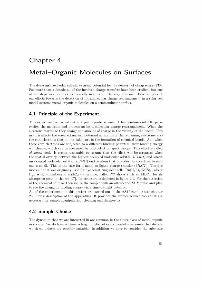
Chapter 4
Metal–Organic Molecules on Surfaces
The dye–sensitized solar cell shows great potential for the delivery of cheap energy [30].For more than a decade all of the involved charge transfers have been studied, but oneof the steps was never experimentally monitored: the very first one. Here we presentour efforts towards the detection of intramolecular charge rearrangement in a solar cellmodel system: metal–organic molecules on a semiconductor surface.
4.1 Principle of the Experiment
This experiment is carried out in a pump probe scheme. A few femtosecond NIR pulseexcites the molecule and induces an intra-molecular charge rearrangement. When theelectrons rearrange they change the amount of charge in the vicinity of the nuclei. Thisin turn affects the screened nuclear potential acting upon the remaining electrons- alsothe core electrons that do not take part in the formation of chemical bonds. And whenthese core electrons are subjected to a different binding potential, their binding energywill change, which can be measured by photoelectron spectroscopy. This effect is calledchemical shift. It seems reasonable to assume that the effect will be strongest whenthe spatial overlap between the highest occupied molecular orbital (HOMO) and lowestunoccupied molecular orbital (LUMO) on the atom that provides the core level to readout is small. This is the case for a metal to ligand charge transfer (MLCT ). The dyemolecule that was originally used for dye sensitizing solar cells, Ru(H2L)2(NCS)2, whereH2L is 4,4’-dicarboxylic acid-2,2’-bipyridine, called N3 shows such an MLCT for itsabsorption peak in the red [97]. Its structure is depicted in figure 4.1. For the detectionof the chemical shift we then ionize the sample with an attosecond XUV pulse and planto see the change in binding energy via a time-of-flight detector.All of the experiments in this project are carried out in the AS3 beamline (see chapter2.2.2 for a description of the apparatus). It provides the surface science tools that arenecessary for sample manipulation, cleaning and diagnostics.
4.2 Sample Choice
The dynamics that we are interested in are common in the entire class of metal-organicmolecules. We do however have a large number of experimental constraints that dictatewhich candidates are possibly suitable. In addition we have to consider the substrate
51

Chapter 4 Metal–Organic Molecules on Surfaces
400 450 500 550 600 650 700 750 800 8500
2000
4000
6000
8000
10000
12000
14000
Wavelength [nm]
Extin
ctio
n Co
e!ci
ent [
1/(c
m m
ol)]
Os"N3N3
N
N
N
Ru
N
N NCS C
S
CO#H
CO#H
CO#H
HO#C
Figure 4.1: N3, the first successfully tested dye for solar cell sensitization. The red linedenotes the absorption curve of N3 while the blue line represents an N3molecule where the ruthenium center has been exchanged for an osmiumcenter. The higher absorption in the near infrared for Os-N3 is caused bythe heavy atom effect which facilitates triplet transitions due to improvedspin-orbit coupling. Osmium also has a higher absorption cross section thanruthenium in the relevant XUV energy range (see figure 4.2). Data adaptedfrom [98].
that our molecules will be resting on. So we have a lot of choice when it comes to theperfect sample for our experiments. Our selection criteria are as follows
• For the excitation we need an absorption band overlapping the NIR pulse centeredat 780 nm
• For efficient detection of the excited state we need an atom in the molecule with acore level that has with a binding energy small enough to be ionized by one XUVphoton and has a large absorption cross section
• The core level has to be chemically shifted during the excitation
• The molecule must be durable enough to withstand pump and probe pulses
• The molecule must stick to the substrate- preferably with covalent bindings thatwithstand considerable laser intensities.
• The substrate cannot have electron emission that spectrally overlaps with that ofthe molecular core level – be it Auger electrons or direct photoemission.
• We have to be able to prepare a clean sample. This includes two points: cleaningthe substrate and subsequently depositing the molecules. If there is a layer ofcontamination on top of the molecules we will not be able to perform the experiment
52

4.2 Sample Choice
because photoelectrons at our typical kinetic energies have a very small mean freepath on the order of a few Angstrom1. We would lose a large part of the signal dueto inelastic electron scattering even with just a monolayer of contamination.
4.2.1 The Substrate
For the substrate we wanted to chose a semiconductor in order to stay close to therelevant system for the technical application. We decided to use silicon in the (111)orientation for several reasons. It is available cheaply and easily in great quality. Thelarge amount of experience in the research community with this material means thatcleaning and handling procedures are readily available. We can functionalize moleculeswith carboxy or hydroxy groups to make them form covalent bonds with the surface.Silicon does not have states that overlap with those of the metal center. Electrons fromthe 2p state at 99.3 eV will be emitted in our experiments, but they are separated inenergy from those of the metal center (see figure 4.4). We do have to be careful to choseour XUV central energy such that we avoid the superposition of our signal with Augeremissions at 92 eV and 107 eV kinetic energy. One way to get around this is to choose acentral XUV energy below the binding energy of Si 2p, which can be beneficial for thetagged molecules discussed in section 4.3.2 and following.
4.2.2 The Molecule
The first candidate for a molecule that comes to mind is the dye that was used in thefirst dye sensitized cell. It is called N3 and is shown in figure 4.1. Let us illustrate theexperimental problems associated with this choice. First of all, the optical absorptioncurve does not match our laser very well. It is suitable for absorption of solar radiationwhich peaks around 500 nm. This wavelength is too short for efficient excitation withour laser system. Secondly, the central metal atom, Ruthenium, has a low absorptioncross section of roughly 0.5Mbarn in the reachable 90 eV to 145 eV photon energy range.For comparison, the solid state experiments that have so far been carried out with ourequipment have mostly been using tungsten as a sample. Its valence band, comprisedmostly of 5d electrons, has a comparable cross section. But a three–dimensional, crys-talline material has a much higher density than the one metal atom in a monolayer ofmetal-organic molecules. So we can expect a signal from ruthenium to be very weak.A less obvious problem with this molecule is its lack of structural solidity. In an idealsituation we would like to deposit a layer of molecules onto a clean surface in ultra highvacuum. This is conventionally done via molecular beam epitaxy (MBE ). In such a sys-tem one brings a reservoir of molecules in front of the surface to deposit them on andthen heats them up in a controlled way. When the temperature surpasses the desorptiontemperature, the molecules will loosen from the reservoir and travel ballistically to thesample surface where they can attach. But If N3 is heated up it has a tendency to break
1See [99] for data on mean free paths of elemental solids. To our knowledge there is no such data forunordered molecular films, but since the qualitative form of the mean free path is so similar for somany different elements we conclude that it will at least follow the same tendency.
53

Chapter 4 Metal–Organic Molecules on Surfaces
80 90 100 110 120 130 140 15010
!1
100
101
102
Ab
sorp
tion
Cro
ss S
ect
ion
[M
ba
rn]
Photon Energy [eV]
I4dMg2pOs4fRu4p
Figure 4.2: Absorption cross sections for a number of suitable candidates as a part ofthe molecular compound to be studied. The cross sections are plotted forthe maximum currently reachable photon energies with our light source. Thedotted vertical lines show the photon energies at which we have performedthe experiments presented in this thesis. Magnesium has been included inthis graph since it has also been tried as a central atom for direct detection-but the cross section is still too low for a time resolved measurement [100].Data taken from [101, 102].
apart before sublimation. This was confirmed by scanning tunneling microscopy studiesperformed at the E20 chair of TUM by Agustin Schiffrin. We believe that this behavior isdue to the structure of the molecule – every part of it hinges on the metal atom througha coordinated binding. In such a bond both binding electrons in an orbital originatefrom the same nucleus. A coordinate of bond can be as strong as a covalent one, but itis typically weaker [93, 103]. When the molecule is heated up the organic parts, whichare only connected through the metal center, can gain enough kinetic energy to tear themolecule apart.When selecting a better sample we can kill two birds with one stone when we try to re-place the central ruthenium atom with an osmium atom. Osmium has a core level withan absorption cross section that is two to four times larger than that of ruthenium (de-pending on the photon energy, see figure 4.2 for an overview of potential candidates’ crosssections). In addition it induces the heavy atom effect [104] in the molecules it is part of.In molecules similar to N3 the absorption in the NIR range of the spectrum is typicallya spin forbidden triplet transition. This is the reason for it being a lot weaker than theabsorption in the blue and UV range. The introduction of a heavy atom strengthensthe spin-orbit coupling and hence increases the absorption strength of triplet transitions[105, 98]. We chose Os2172, which is shown on figure 4.3 [106]. It is very similar toOs-N3, but it has an absorption curve that fits better to our laser system.
54

4.3 Steady State Experiments
x10!
300 400 500 600 700 800 9000
0.5
1
1.5
2
2.5
3
3.5
Wavelength [nm]
Extin
ctio
n co
e"ci
ent [
1/M
cm]
NN
N
NN
CF#
Os
N
N
N
HOOC
HOOC
HOOC
CF#
Figure 4.3: Os2172, another compound used for solar cell sensitization. The organic partsof the molecule are bound through coordination bindings with an osmiumatom at its center. The presence of a heavy atom leads to stronger absorptionbands in the NIR range through the the heavy atom effect. In addition, theabsorption cross section in the XUV is higher for osmium than for ruthenium,as present in N3.
4.2.3 Sample Preparation
In the first step we cleaned the silicon substrate by sputtering and annealing in vacuum.The cleanliness was checked with X-ray Photoelectron Spectroscopy (XPS).For the deposition of the molecule we chose a method that took the fragility of themolecule into account. We took a clean slide of Silicon in the (111) orientation and puta drop of ethanol containing 1.8⇥ 10�3
m Os2172 on it. Then we waited for it to almostevaporate and put another drop on top and so forth. A typical preparation procedureinvolved roughly 30 to 50 drops. We put so many individual drops onto the surfacebecause we wanted to be sure to have a thick layer of molecules on the sample for thefirst experiments. Once the thick layer is successfully detected we can move on to acontrolled monolayer. We could not create a more concentrated solution due to the poorsolubility of Os2172 in common solvents. The entire procedure was carried out in afumehood, then the sample was transferred to vacuum.
4.3 Steady State Experiments
4.3.1 Direct Observation of the Metal Center: Os2172
X-Ray Photoelectron Spectroscopy of Os2172
In order to characterize the molecular layer on the sample we performed X-ray Photo-electron Spectroscopy (XPS) with an aluminum K-↵ cathode at 1486 eV [70]. The resultsare shown in figure 4.4. We can clearly identify the main peaks of the spectrum with the
55

Chapter 4 Metal–Organic Molecules on Surfaces
0 200 400 600 800 1000 1200100 300 500 700 900 1100Binding Energy [eV]
Phot
oele
ctro
n Si
gnal
[a.u
.]
O KLLF KLL
F1sO1s
N1sC 1s
Si 2s
Os4d
N KLL
0
0.2
0.4
0.6
0.8
1
Si 2p
Os 4f
53 99
Figure 4.4: XPS spectrum of Os2172 on Si(111) acquired with an Al K-↵ X-ray cathodeat 1486 eV. The visible peaks are identified as the characteristic spectra ofthe constituents of the molecular adlayer. Hydrogen, whose absorption crosssection is very low, cannot be detected in XPS.
help of research databases available online [71] and map them onto the constituents ofour molecule. Typically this method is also used to check the cleanliness of a sample. Itcan easily detect small amounts of contamination on an otherwise flat background. Thisworks very well for substrates without organic adlayers. In our case however it is morechallenging to identify organic contaminants because the molecule that we deposited onthe surface already has all the typical components of such compounds. We can howevercompare the peak areas corresponding to a molecular signal to those that might alsobe coming from a contaminant (such as the carbon 1s peak) and see whether the ratiobetween them matches the one we would expect from the stoichiometry of the molecule.In the case of drop-deposited Os2172 we have to make another concession. The thicknessof the adlayer is very uneven – to the extent that this is clearly visible by the naked eye.At the same time we can still see a signal from the substrate core levels. So the adlayer isvery thin in parts and very thick in others. As the mean free path for electrons changeswith kinetic energy we would normally have to consider it when comparing the afore-mentioned peak areas at different kinetic energies. This is unfortunately not possible forthe greatly varying layer thickness and will be neglected.For Os2172 we compared the peak area of the carbon 1s at 285 eV level to that of fluorine1s at 687 eV. Fluorine is not abundant in the laboratory environment and is used as aproxy for the molecule whereas carbon is a part of any organic contamination and servesas a proxy for a signal from both the molecule and the contamination layer. From thecross sections we would expect the ratio to be (C1s/F1s)theory ⇡ 1.1. In the measurementwe get a ratio of (C1s/F1s)experiment ⇡ 1.5. This would mean that there is more carbonthan expected on the surface, hinting at a contamination layer.
56
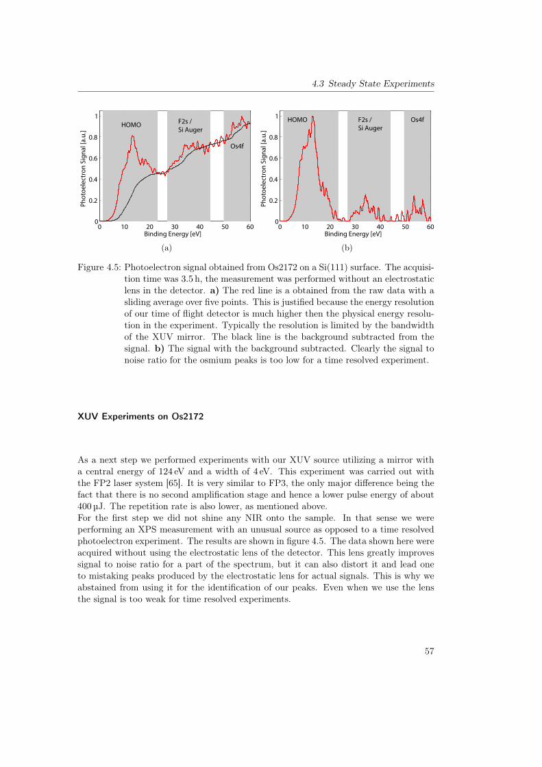
4.3 Steady State Experiments
0 10 20 30 40 50 600
0.2
0.4
0.6
0.8
1HOMO F2s /
Si Auger
Os4f
Phot
oele
ctro
n Si
gnal
[a.u
.]
Binding Energy [eV]
(a)
0 10 20 30 40 50 600
0.2
0.4
0.6
0.8
1 HOMO F2s /Si Auger
Os4f
Phot
oele
ctro
n Si
gnal
[a.u
.]
Binding Energy [eV]
(b)
Figure 4.5: Photoelectron signal obtained from Os2172 on a Si(111) surface. The acquisi-tion time was 3.5 h, the measurement was performed without an electrostaticlens in the detector. a) The red line is a obtained from the raw data with asliding average over five points. This is justified because the energy resolutionof our time of flight detector is much higher then the physical energy resolu-tion in the experiment. Typically the resolution is limited by the bandwidthof the XUV mirror. The black line is the background subtracted from thesignal. b) The signal with the background subtracted. Clearly the signal tonoise ratio for the osmium peaks is too low for a time resolved experiment.
XUV Experiments on Os2172
As a next step we performed experiments with our XUV source utilizing a mirror witha central energy of 124 eV and a width of 4 eV. This experiment was carried out withthe FP2 laser system [65]. It is very similar to FP3, the only major difference being thefact that there is no second amplification stage and hence a lower pulse energy of about400 µJ. The repetition rate is also lower, as mentioned above.For the first step we did not shine any NIR onto the sample. In that sense we wereperforming an XPS measurement with an unusual source as opposed to a time resolvedphotoelectron experiment. The results are shown in figure 4.5. The data shown here wereacquired without using the electrostatic lens of the detector. This lens greatly improvessignal to noise ratio for a part of the spectrum, but it can also distort it and lead oneto mistaking peaks produced by the electrostatic lens for actual signals. This is why weabstained from using it for the identification of our peaks. Even when we use the lensthe signal is too weak for time resolved experiments.
57

Chapter 4 Metal–Organic Molecules on Surfaces
200 300 400 500 600 700 8000
100
200
300
400
500
600
Wavelength [nm]
Abso
rptio
n [a
.u.]
N
N
N
OsN
NN
IHO
Figure 4.6: MBM4179, a compound specifically synthesized for time resolved experimentsby Majewski and Wolf [107].
4.3.2 Iodine Tagging: MBM4179
We can see that is not possible to perform the desired experiments with Os2172 as asample. Equally we can deduce that studying the metal center directly is unlikely to bepossible since Osmium was already selected for its high cross section. There is anotherpossibility to study charge rearrangement within such molecules: we can attach a tagatom to the molecule that has a core level with a high absorption cross section. Thenwe probe said core level and observe its chemical shift. Naturally the question ariseswhether such an extra atom would be affected by charge rearrangement and whetherit would experience such an observable chemical shift. There have been reports on thesuccessful detection of a shift on the order of 3 eV on a molecule tagged with iodine[15]. In this specific case there is no large spatial charge rearrangement in the molecule(as opposed to the previously considered case of a metal to ligand charge transfer), butthe electronic configuration of the iodine atom is still sensitive enough to it to exhibit adetectable shift. So our next sample choice was a tagged molecule: MBM4179, shownin figure 4.6. It was synthesized for our experiments as part of a collaboration withMarek Majewski and Michael Wolf from the University of British Columbia [107]. Themolecule is functionalized with a hydroxy group for surface attachment and a iodophenylgroup for tagging. In its ground state the molecule is doubly positively charged. In orderto counter this charge there are two negatively charged PF6 molecules per MBM4179present in the sample.
X-Ray Photoelectron Spectroscopy of MBM4179
We prepared the samples for our XUV photoelectron experiments in a way similar toOs2172 and performed an XPS measurement. This time the molecule was depositedfrom a 1⇥ 10�4
m acetonitrile solution with 40 drops. This yielded the data shown infigure 4.7. The XPS data also reveals the presence of the above mentioned counterions.
58

4.3 Steady State Experiments
0 100 200 300 400 500 600 700 800 9000
0.2
0.4
0.6
0.8
1
Binding Energy [eV]
Phot
oele
ctro
n Si
gnal
[a.u
.]
C 1sO1s
N1s
I4sI4p
I3d F1sF KLL
P2s
I4d /
Os4f
55
F2s
Figure 4.7: XPS data of MBM4179. The constituents of the molecule are clearly dis-cernible. The F1s peak is split up in two. Since this is a level with an angularmomentum of zero it cannot be a spin orbit splitting but rather a chemicalshift. This indicates that the fluorine must be subect to two different sur-roundings – either binding to different atomic species or at different sites.The spin-orbit splitting of Os4f is not clearly visible anymore because theOs4f level overlaps with the I4d level. At 93 eV the cross section of Os4fwill be roughly 17 times smaller than that of I4d and thus this will not be aproblem for the actual experiment.
We compared the peak area of C1s as a proxy for a superposition of contaminationand molecular signal to that of I3d (originating only from the molecule) to judge thecleanliness of the surface. The XPS data shows no peaks from the substrate so we canconclude that there is layer on top of the substrate which is thick enough for us to includethe mean free path into our considerations as discussed for Os2172. The expected valuefrom the cross sections and mean free path was (C1s/I3d)theory ⇡ 0.7, while the measuredvalue was (C1s/F1s)experiment ⇡ 2.2. Here we can again clearly see from the higher carboncontent that there is a contamination layer in addition to the deposited molecules.
XUV Experiments on MBM 4179
Even if the sample can not be prepared in a clean way we can still learn something from it.When we expose it to XUV radiation we can try and find out whether the signal to noiseratio for the iodine 4d peak that we would be studying is high enough for time dependentexperiments. If this is the case for a dirty sample then it is certainly true for a clean one.Just like for Os2172 we performed the measurement without an electrostatic lens in ordernot to change the spectrum in the observation. For these experiments we again used theAS3 beamline, but in this case we employed the FP3 laser system described in 2.2.1. Itsrepetition rate of 4 kHz is larger than that of FP2 with 3 kHz. Also its pulse energy ismore than twice as high. This leads to much higher flux of XUV photons and to a cutoff
59
Chapter 4 Metal–Organic Molecules on Surfaces
at higher photon energies. It is actually challenging to produce isolated XUV pulses atphoton energies around or below 100 eV. When measuring with iodine tagged atoms itis however necessary to do so because its absorption cross section increases dramaticallywhen reducing the photon energy (see figure 4.2). We chose a mirror at 93 eV with awidth of 4.5 eV as a compromise between the cross section and the possibility of creatingisolated pulses. In the measurements that we took we have seen strong modulation inthe XUV photon spectrum in the energy range of our mirror so we are not working withisolated pulses. This does not change the validity of our experimental findings as we donot perform time dependent measurements in the first step.An additional factor that needs to be considered is related to the central energy of thephotoelectrons obtained from the I4d level. Its binding energy is roughly 55 eV. Whenwe are working with 93 eV photons that yields a kinetic energy of 38 eV. This is alreadyquite low and limits the intensity of a NIR pump pulse as the high energy edge theelectron background can reach energies similar to that of the photoline and overwhelmthe signal. So even if an isolated XUV pulse could be achieved at lower energies it isadvisable to stay at energies around 90 eV in order to be able to pump efficiently.The data we obtained is shown in figure 4.8. As is to be expected from the factorsexplained above (lower photon energy, higher NIR pulse energy, higher repetition rate,higher cross section) the acquisition time was significantly lower at six minutes comparedto over three hours for Os2172. But in addition it is apparent that the iodine signal ismuch more discernible than the osmium signal was. It seems that even though the sampleis not perfectly clean and there is probably a contamination layer the iodine cross sectionis high enough for a time resolved experiment.The natural next step was to try a pump-probe experiment on the molecule. Evenwithout isolated attosecond pulses it is possible to perform a time resolved experiment– it merely deteriorates the temporal resolution to the duration of the envelope of thepulse train as opposed to the duration of one single pulse. Unfortunately we were notable to see a time dependent signal. Possible reasons for the lack of signal included:
• Possible instability of the coordination binding when exposed to laser radiation atthe intensities needed to see an excitation (we increased the intensity up slowly andscanned at different intensities without seeing a signal)
• Signal deterioration through the contamination layer
• Too small optical extinction of the molecule
With our next sample choice we aimed to remedy these points.
4.3.3 Iodine Tagging and Evaporation Deposition: Tetraiodo CopperPhthalocyanine
After learning that iodine tagging produces a detectable signal suitable for time depen-dent experiments and that a clean preparation scheme is very beneficial for the inter-pretation of any data we selected a molecule that fulfills our refined criteria: Tetra-Iodo
60

4.3 Steady State Experiments
0 10 20 30 40 50 600
0.2
0.4
0.6
0.8
1HOMO F2s I4d
Binding Energy [eV]
Phot
oele
ctro
n Si
gnal
[a.u
.]
(a)
0 10 20 30 40 50 600
0.2
0.4
0.6
0.8
1HOMO F2s I4d
Binding Energy [eV]
Phot
oele
ctro
n Si
gnal
[a.u
.]
(b)
Figure 4.8: Photoelectron spectrum of MBM4179 on Si(111) obtained with XUV photonsat 93 eV with a width of 4.5 eV. a) Spectrum with background b) Backgroundsubtracted. It is apparent that the signal to noise ratio and the signal tobackground ratio are sufficiently high for a time resolved experiment.
Copper Phthalocyanine (I4CuPc), depicted in figure 4.9 along with its optical extinctioncoefficient in a dimethyl sulfoxide solution. In the previously used molecules the transi-tions of interest were metal to ligand charge transfers. The charge transfer lines on thesemolecules in the near infrared are spin forbidden and have a very low extinction coeffi-cient of a few thousand L cm
mol at most. This is not the case for I4CuPc. The absorptionline at 600 nm to 700 nm that overlaps with our light source corresponds to a transitionbetween the ⇧-type HOMO and LUMO orbitals that are located on the aromatic ring[108]. This is potentially problematic since the charge density in the proximity of ouriodine tags changes very little between HOMO and LUMO. Whether or not this changewill be result in a detectable chemical shift remains to be determined.In contrast to the molecules that we used in the previous experiments Phthalocyanineshave a closed aromatic structure around the metal center. The aromatic part is notbound through coordination bindings to the metal center but through more stable cova-lent bindings. This makes it possible to evaporate Phthalocyanines and deposit them ina very clean and controlled way [109]. Whether or not this is true for the iodine taggedversion that we are studying is a question that can and will be answered by scanningtunneling microscopy and scanning tunneling spectroscopy experiments [110].
X-Ray Photoelectron Spectroscopy of I4CuPc
Figure 4.10 shows an XPS spectrum of I4CuPc deposited on Si(111) via evaporation.When performing the same analysis as for the other two studied molecular species wechose to compare the peak areas of carbon 1s and iodine 3d. We would expect a ratio of(C1s/I3d)theory ⇡ 0.2, whereas we are seeing (C1s/I3d)experiment ⇡ 0.025. The iodine signal isone order of magnitude larger than expected. We also compared the iodine 3d level to the
61

Chapter 4 Metal–Organic Molecules on Surfaces
300 400 500 600 700 800 900 10000
5000
10000
15000
Wavelength [nm]
Extin
ctio
n Co
e!ci
ent [
L/(c
m m
ol)]
NN
N N
N
N
N
N Cu
I I
I
I
Figure 4.9: The optical absorption of tetraiodo copper phthalocyanine in dimethyl sulfox-ide with a concentration of 1.44 mmol
L . The strong absorption around 600 nmcorresponds to a HOMO-LUMO transition between ⇧-type orbitals on theorganic ring [108]. Spectra courtesy of [111]. The inset shows the structureof I4CuPc.
copper 2p1/2 level. The 2p3/2 peak overlaps with the iodine 3p1/2 peak. We adjusted thecross sections to account for the fact that we are only studying one of the two spin-orbitsplit levels. The expected result was (I3d/Cu2p)theory ⇡ 5.4 and the measurement yielded(I3d/Cu2p)experiment ⇡ 6.4. This is not exactly the stoichiometrically expected ratio but itis not nearly as far off as the ratio between carbon and iodine.Combining the two comparisons tells us that there is no evidence for organic contamina-tion on the sample – in contrast, there is a shortage of carbon. There might have beena contamination on the substrate from previous molecule preparations that could not becompletely removed. When the sample is sputtered, the molecule can break apart andnot all constituents stick to the surface in the same way.
XUV Experiments on I4CuPc
The first spectra of I4CuPc at a photon energy of 95 eV are shown in figure 4.11. Wecannot be certain that the large and well visible iodine peak exclusively stems from intactmolecules, but it seems encouraging. Even if we can completely follow the XPS analysisand the molecular signal were one order of magnitude lower than measured here it wouldstill be detectable. In addition it is possible to lower the photon energy even further andgain signal strength through the increasing cross section of iodine. At 90 eV it is already50% higher and at 85 eV it increased more than twofold compared to our current workingpoint of 95 eV. This would make obtaining an isolated pulse more challenging, but it willstill be feasible according to our experimental experience.
62

4.3 Steady State Experiments
0 200 400 600 800 1000 1200
0.5
1
1.5
2
2.5
3
3.5
Binding Energy [eV]
Phot
oele
ctro
n Si
gnal
[a.u
.]
C1sN1s
I3dCuLMM
Fe (from sample holder)
Si2sSi2p
I3p 1/2
I MNN
I3p 1/2
Cu2p 3/2
Cu2p 1/2
N KLL
50 99
I4d Si2p
Figure 4.10: XPS spectrum of I4CuPc deposited via evaporation in vacuum. The smallpeaks at 750 eV and 800 eV arise from the sample holder that contains steel.
0 10 20 30 40 500
0.2
0.4
0.6
0.8
1HOMO I4d
Phot
oele
ctro
n Si
gnal
[a.u
.]
Binding Energy [eV]
(a)
0 10 20 30 40 500
0.2
0.4
0.6
0.8
1HOMO I4d
Phot
oele
ctro
n Si
gnal
[a.u
.]
Binding Energy [eV]
(b)
Figure 4.11: An XUV spectrum of I4CuPc acquired at a photon energy of 95 eV. Thisspectrum was acquired in merely three minutes without an electrostaticlens. Comparing this to Os2172 and MBM4179 demonstrates in stark con-trast that the quadruple iodine tag in combination with a clean preparationscheme yields superior results. The signal is definitely strong enough fortime resolved experiments.
63

Chapter 4 Metal–Organic Molecules on Surfaces
4.4 Conclusions
We can draw these main conclusions from our experiments so far:
• The direct observation of a metal center in a thin layer of metal organic moleculesis not possible with our setup. With a drastically increased XUV flux it could bean option in the future, but at the moment it is out of reach.
• An ex-situ preparation which involves removing the sample from vacuum and thedepositing the molecular sample on it will result in a contamination of the sample.The influence of this contamination cannot easily be quantified.
• If we want to avoid contaminations in our samples we have to deposit them invacuum. Evaporation, presenting the cleanest and most controlled option, is onlypossible for molecules that are not held together via coordination bindings to thecentral metal atom. This rules out a large subset of metal-organic molecules forour experiments.
• The observation of an iodine tag attached to a molecule is possible at photonenergies around 90 eV.
4.5 Outlook
A challenge that has to be overcome is the clean and controlled preparation of an iodine-tagged phthalocyanine. In order to control all experimental parameters we do not onlyplan to perform XPS measurements but also scanning tunneling microscopy and scanningtunneling spectroscopy after a deposition through evaporation. With these techniquesit is possible to determine the spatial orientation and structural integrity of molecularadlayers on semiconductors. Another possible problem lies in the hitherto unknownstrength of the coupling between the orbitals involved in a ⇧–⇧⇤ transition with theiodine core levels. It is conceivable that a transition takes place but cannot be observeddue to the large spatial separation between iodine tag and central ⇧-type electronicsystem. The experiments of Dachraoui et al. [15] do make it seem plausible, but anexperimental proof has yet to be provided.
64

Chapter 5
Attosecond Delay Spectroscopy onTungsten
Electronic transport in solids is a fundamental phenomenon that has a multitude of appli-cations in electronics. The ongoing miniaturization of transistors leads to an increasinginterest in electronic motion on the angstrom length scale. With the help of attosecondstreaking we can monitor electronic transport through few atomic layers on an ultrashorttimescale. In the past years the first first such findings of Cavalieri et al. [20] have beengreatly refined. Here we present the extension of the streaking technique towards higherXUV photon energies and a summary of past measurements.
5.1 Principle of the Experiment
The basic idea of delay spectroscopy is an extension of the streaking method. As ex-plained in section 2.1.3 this technique directly measures the vector potential of an intensepulse. In the discussion so far we have assumed that there is a target material that pro-vides us with a state that we can photoionize to produce free electrons. But for somematerials there is more than one state in the accessible energy range. If we photoionizetwo or more states in our experiment we get a curve resembling the vector potentialfor each of those states respectively. An example is given in figure 5.1. This data wasacquired with XUV pulses centered at 145 eV with a spectral FWHM of 4.5 eV and atemporal duration of 480 as on a tungsten (110) surface. The two lines from the valenceband and the 4f level are clearly discernible1. When we are streaking two lines bothof the traces will represent the vector potential of the same NIR laser field. But thereare still some things that can differ between the two. Since we are dealing with a solidhere we have to consider whether the photoelectrons that we are studying are currentlywithin the material or without. Inside the tungsten medium the streaking amplitude
1Actually there are more than two levels: the W4f is split up into W4f5/2 and W4f7/2. Both of theselevels are split in a bulk and a surface contribution. There is also the additional W5p level very closeby. But as all these levels are separated by less than the bandwidth of our XUV mirror (4.5 eV) thelines can not be easily separated any longer. In the analysis it is assumed that they have the sametemporal structure for the TDSE evaluation. This is justified by the absence of interference betweenthem. Since the W5p cross section is significantly smaller than that of W4f in the photon energyrange discussed here we will refer to the photoline simply as the W4f line. A similar rationale appliesto the other photoline that we will call the valence band from here on.
65

Chapter 5 Attosecond Delay Spectroscopy on Tungsten
!3 !1 1 3
100
110
120
130
140
150
P
hoto
ele
ctro
n K
inetic
Energ
y [e
V]
delay [fs]
0
0.2
0.4
0.6
0.8
1
(a)
100
110
120
130
140
150
Phot
oele
ctro
n Ki
netic
Ene
rgy
[eV]
delay [fs]
0
0.2
0.4
0.6
0.8
1
!3 !1 1 3
(b)
Figure 5.1: a) A streaking spectrogram of tungsten acquired with a central photon energyof 145 eV. The line at higher kinetic energies corresponds to the valence bandwhile the line at lower kinetic energies corresponds to the 4f level of tungsten.The black line shows the result of a center of energy analysis. The whiteline denotes that above this line the spectrogram has been multiplied by 5for better visibility. b) The reconstructed spectrogram, a result of a TDSEanalysis of the data on the left. The chirp is qualitatively well reproducedin both lines. The challenge for both methods is in the discrepancy of signalstrengths between the two lines. This will be discussed in detail in section5.3.
will be reduced by a factor of ⇡ 16 [20]. Consequently, we are only effectively streakingelectrons from the point in time when they reach the surface. If the electrons from thetwo different states leave the medium at different times they are exposed to a differentfield and their traces will be shifted on the delay axis with respect to each other.This finding was first reported by Cavalieri et al. in 2007 [20], who discovered that thevalence band emission in tungsten precedes the 4f core level emission in tungsten by(110± 70) as. This result was groundbreaking and opened the door for a number ofpossible theoretical explanations, which will be summarized in section 5.2. And yet theunderlying data had major limitations: There is only one data point, generated by twomeasurements with relatively high uncertainty. The theoretical considerations yieldedmultiple possible physical origins of the delay that all fit this data point. In the last fewyears a series of experiments were performed that were designed to confirm or rule outthe hypotheses provided by theory.
66

5.2 Theoretical Considerations
5.2 Theoretical Considerations
As mentioned in the previous section, there are a number of theoretical explanations forthe measured delays in photoemission from solids so far. There have also been summariesof these publications in these sources: [69, 112]. The following table is intended to givea short and concise overview of the current status of calculations.
Physical explanation fordelay
Used methods, assump-tions
results, prediction
Cavalieri et al., 2007 [20]
Final state band structurewithin metal, different es-cape depths
Static band structure inexcited state. Does nottake photoexcitation intoaccount: no selection rulesand no transition proba-bilities for the individualtransitions considered
Works for 90eV: predicts90as
Zhang and Thumm, 2009 [113]
Interference effects in the4f line due to photoemis-sion from distinct depths.Valence band is delocalizedand does not show this be-haviour.
One step quantum me-chanical photoionizationcalculation. Penetrationdepth of NIR much largerthan escape depth ofelectrons
Delay depends on meanfree path of 4f electrons,which changes with photonenergy.
Lemell et al., 2009 [114]
Group velocities, emis-sion depths, scatteringprocesses that slow VBelectrons to 4f energy
Semiclassical Ansatz; clas-sical transport theory withquantum scattering prob-abilities; influence of theNIR pulse on the pri-mary photoexcitation pro-cess and local crystal-fieldeffects on the emission timespectrum neglected
Predicts 42as delay at 90eV
Kazansky and Echenique, 2009 [115]
Different localization char-acteristic for different ini-tial states; no band struc-ture effect because staticband structure does notapply at these time scales
1D TDSE; neglects hole invalence band
Predicts result at 90eV cor-rectly within error mar-gins: 85as
67

Chapter 5 Attosecond Delay Spectroscopy on Tungsten
Krasovskii, 2011 [116]
Final state effect caused byband structure
Assumes normal emission;1D calculation
Strong variation with pho-ton energy predicted
Zhang and Thumm, 2011 [117]
Different Localizationcharacteristic for differentinitial states
Field penetration depth setto zero; 1D model surfacewith core potentials of dif-ferent widths to representlocalization
120as at 90eV
Neppl, 2012 [69]
Free electron transport Free Electron- like disper-sion assumed. Mean freepaths from [99]
Predicts delay vs photonenergy curve; delay toosmall at 95eV and a bit toosmall at 118eV; right forlarger energies
Borisov et al., 2013 [118]
Surface vs bulk: resonantemission in bulk vs nonres-onant emission at surface;Amount of surface contri-bution to photoline playslarge role in delay.
1D model potentials withvarying harmonics contentwhich allows/forbids reso-nant interband transitionsfor core/valence levels
Explains experiments onMg (see next paragraph);predicts right delay forW110 at 90 eV
So far none of these publications is predicting our experiments precisely. Some of theidentified problems include:
• Cavalieri et al., 2007 [20]:Offers a very simplistic approach that neglects the entire photoexcitation process.
• Zhang and Thumm, 2009 [113];Zhang and Thumm, 2011 [117] andKazansky and Echenique, 2009 [115]:These studies conclude that the origin of the observed delay is given by differentlocalization property of the initial states: a localized core state (4f) versus a de-localized valence band. If this were the case then it would have to occur also inother materials when comparing localized with delocalized levels. There has beena study on the (0001) surface of magnesium at a photon energy of 118 eV whichfound no appreciable delay between the delocalized valence band and the localized2p level [69], even though the valence band of magnesium is delocalized to a higherdegree than that of tungsten [119, 120]. In the free-electron metal magnesium thevanishing delay can be explained with free electron dispersion.
• Lemell et al., 2009 [114]:Provides a value for the delay at 90 eV that was inside the error bars for the very
68
5.3 Past Measurements on Tungsten and O/W
first dataset of Cavalieri et al. It’s prediction of 42 as is now safely outside the errorbars.
• Neppl, 2012 [69]:Assumes free electron dispersion as the cause for the delay. The predicted delayversus photon energy is shown in figure 5.2. It evidently does not match theexperimental data.
• Borisov et al., 2013 [118]:The main finding here is given by the idea that the ratio between emission fromsurface states and bulk states determines the delay. The measurements for W(110)at 90 eV and for Mg (0001) at 118 eV can be reproduced. This is a promisingapproach. It should be considered that there have been measurements on cleantungsten (110) with an added layer of hydrogen [112], which report a very similardelay value to clean tungsten. There are reports claiming that the adlayer stronglyreduces the contribution of surface states to the photoemission [121]. This analysisof Feuerbacher and Fitton is likely incomplete since it only takes surface states intoaccount that emit perpendicularly to the surface. Angularly resolved studies showthat the hydrogen layer shifts the surface state photoemission towards the edges ofthe Brillouin zone [122]. Since we are integrating over a large angle of ca. ±20� wecan still detect those states.
• Krasovskii, 2011 [116]:Concludes that the effect is caused by a final state effect: the band structure ofW(110) above the Fermi edge. It predicts a much smaller delay for measurementsat 105 eV than at 90 eV. This has not been observed experimentally. In additionthere have also been measurements on a different crystal orientation of tungsten:W(100) at 105 eV. Since the band structure depends on the orientation, the delayshould also vary between these two samples – but it is not measurably differentbetween W(100) and W(110).
It is evident that the attosecond dynamics of tungsten still pose a conundrum and nosingle theoretical ansatz was able to fully explain them.
5.3 Past Measurements on Tungsten and O/W
The W(110) surface has been extensively studied at the Max–Planck–Institute for Quan-tum optics for several years. In this work we have built on the gathered experience, usedthe same sample preparation techniques that have been reported by Neppl [69] and willreport on them only briefly. For the clean surface we performed alternating sputteringand annealing cycles after bringing the sample to vacuum. That leaves mostly carbonas a possible contaminant, which is removed by flashing the sample to 2400K in an oxy-gen atmosphere. This makes the carbon desorb as carbon monoxide. Then the sampleis flashed to 2400K again to get rid of possible oxygen remnants. We also performedmeasurements on an oxygen overlayer in the (1 ⇥ 1) reconstruction on tungsten. This
69

Chapter 5 Attosecond Delay Spectroscopy on Tungsten
90 95 100 105 110 115 1200
50
100
150
XUV Photon Energy [eV]
VB
! 4
f D
ela
y [a
s]
Clean W(110)Free electron dispersionO(1x1)!W(110)
Figure 5.2: An overview of the measurements on clean W(110) and O/W that have beenperformed prior to this thesis. It seems like the delay is sloping downwards asthe photon energy of the XUV beam is increased. The error bars represent thestandard deviation of the data. The delay calculation for W(110) assumingfree electron dispersion in the metal is shown as the blue dashed line. Apositive number in the delay indicates that the valence band electrons arrivefirst [69, 123].
60 70 80 90 100 110 120 130 140 150 16010
!2
10!1
100
101
Photon Energy [eV]
Ab
sorp
tion
Cro
ss S
ect
ion
[M
ba
rn]
W4fW5dO2p
Figure 5.3: The cross sections of the relevant levels for tungsten delay spectroscopy: W4fand W5d/O2p (the chief contributions to the valence band of the clean tung-sten and O/W surfaces). These values are calculated and not necessarilyapplicable to the highly surface sensitive spectra that we are acquiring. Theywill however reproduce the general trend quite well, which is sufficient tosupport our argument. On the logarithmic scale of the absorption cross sec-tion it becomes apparent that observing both tungsten levels simultaneouslygets increasingly difficult at higher photon energies. The cross section of O2pdominates the valence band line of O/W for the energy range relevant to ourapplication. Measurements have been performed at the photon energies thatare indicated as dotted lines [102, 101].
70

5.3 Past Measurements on Tungsten and O/W
will be referred to as O/W from here on. For its preparation we expose the sample to anoxygen atmosphere of 1⇥ 10�5 mbar for 10 minutes after the standard cleaning steps.Figure 5.2 shows the available data points on the photoemission delay of W(110) andO/W before the implementation of the FP3 laser system. From these points we wouldhave to assume the delay to steadily decrease with increasing energy – possibly with alinear or quadratic slope. This would hint at a relatively simple explanation as opposedto a band structure effect that could be expected to exhibit a more complex dependence.But this is simply caused by the low number of data points, not by their values. In orderto provide a better data basis for theoretical explanations we looked into the feasibilityof more scans at different photon energies. There are three main obstacles to overcomefor this endeavor:
• The cross section of tungsten must be high enough over the entire range for anexperiment.
• The cross sections of the two involved photolines must not differ by too much. Fig-ure 5.3 shows how the relevant cross sections change with photon energy. Towardslower energies the cross sections are similar and both high enough for experiments.Conversely, increasing the photon energy severely reduces the cross section of thevalence band. At 145 eV the difference between the two lines is already a factor of100. It is challenging to simultaneously measure two lines that differ by this muchin their signal strength. The specific challenges of this measurement will be shownin section 5.4
• The isolated XUV photons must be produced with our high harmonic generationsetup. With the standard Femtopower laser systems the XUV range in which onecan generate enough photons for a time dependent experiment extends from 90 eVto 135 eV. At the edges of this range it gets exceedingly difficult to produce anadequate number of isolated photons – at the lower end one typically producespulse trains and at the higher end there are no more photons. With the newlyimplemented booster system it is possible to extend this range to higher energies,as will be discussed in section 5.4.
For the measurements on O/W the situation is different. Here the cross sections are notdiverging as fast as for the clean metal. But the data interpretation is more complicateddue to the layered structure of the sample. The emission from the oxygen adlayer andthe top tungsten layer are not distinguishable since the valence orbitals of both elementsare responsible for the binding and form overlapping bands [69, 124]. Qualitatively thelarger delay values for O/W than for clean W(110) can be explained by two factors:the emission depth and the temporal effect of the charge density at the O/W interface.The cross section for the O/W valence band is dominated by the surface contribution ofthe adlayer and the top tungsten layer whereas the 4f electrons can only emerge fromthe interface or below. This shifts the center of gravity of the emergence of valenceband photoelectrons closer to the surface and makes them arrive earlier in the streaking
71

Chapter 5 Attosecond Delay Spectroscopy on Tungsten
90 100 110 120 130 140 1500
0.2
0.4
0.6
0.8
1
Photon Energy [eV]
Inte
nsity
[a.u
.]
FP2, without booster stageFP3, with booster stage
Figure 5.4: Typical XUV spectra for a Femtopower based system without a booster stage(FP2, blue dashed line) and with a booster stage (FP3, red line, see figure2.5). Both spectra have been normalized. The experimentally usable photonenergies for the booster system extend up to ⇡ 150 eV. The inset showsthe beam profile as recorded on the MCP detector behind the experimentalchamber of AS3 (see figure 2.10). The white ring indicates the circumferenceof the pellicle/wirecross filter in the final chamber of the AS3 beamline (seefigure 2.9). The part of the mode that passes through this filter is usable inthe experiment. Evidently almost the entire intensity is captured within thisaperture.
field. Additionally the short binding length of O/W 2 leads to a higher charge density atthe interface that affects the temporal properties of the emitted electrons. This is hardto quantify but it will affect the slower electrons from the 4f levels more strongly anddelay them further. The higher delay values for the O/W measurements than for cleantungsten confirm these expectations.
5.4 Production and Characterization of High Harmonics at145eV
As mentioned in the previous section the interpretation of our experiments on tungstenwould greatly benefit from a data point at higher XUV photon energy. According toequation 2.6 the higher pulse energy provided by an additional booster stage in FP3should translate to an increase in photon energy. Whether or not the calculated param-eters can actually be reached experimentally is a more difficult question, since the pulselength varies between the laser systems and the response of the neon gas used for high
2Roughly 1Å for the O/W bond compared to the tungsten lattice constant of roughly 3Å. In the bcccrystal of tungsten this translates to a next neighbor distance of ⇡ 2.6Å.
72

5.5 Delay Spectroscopy of Tungsten and O/W at a Photon Energy of 145eV
harmonic generation is complex. The output of FP3 is not as well compressed as theone of FP23 and hence the present slight pre-pulse contributes to ionization of the targetmedium, which greatly diminishes the XUV yield of following laser cycles. Also the non-optimal compression reduces the maximally achievable electric field, which in turn limitsthe XUV photon energy. Our experimental findings are shown in figure 5.4. We focusedthe beam with a spherical mirror with a focal length of 60 cm into a quasistatic gas cellcontaining 200mbar Neon gas and optimized the spectrum on the high energy end. TheFP2 spectrum was obtained with a 40 cm focusing length and similar gas pressure. Herewe can see that the standard Femtopower systems are not able to generate intense har-monics above 130 eV. It is challenging, but possible to perform streaking spectroscopywith these lasers on tungsten surfaces at 135 eV – albeit at reduced count rates. Formeasurements at higher energies, the booster system of FP3 enables an extension of therange by roughly 15 eV up to ⇡ 150 eV. We chose a compromise between photon numberand energy by utilizing an XUV mirror at 145 eV with a spectral FWHM of 4.5 eV. Thiswould support an XUV pulse length of 400 as if there was no dispersion. Comparing theabsolute count rates between the systems is challenging. The XUV beam has to passthrough filters and is reflected off mirrors at grazing incidence. These optical elementsfrequently deteriorate when we expose them to intense laser radiation. Such a deterio-ration can easily diminish the XUV flux by 30% to 50% for one optical element. For areliable measurement one would have to compare the two different laser systems in thesame beamline in direct succession, which was not done. FP3 drastically improves theelectron count rates for high photon energies above 120 eV. This is due to the highertotal energy that allows us to employ longer focusing lengths and larger beam diametersat the high harmonic generation. In this way we can reach the optimum intensity ina larger volume and create more XUV light. The total count rates are also improvedsimply by the higher repetition rate of FP3: It runs at 4 kHz compared to the 3 kHz ofFP2. Another remarkable property of the created harmonics is their stability. In typi-cal performance we measured around 1% RMS intensity fluctuation over a time of onesecond.
5.5 Delay Spectroscopy of Tungsten and O/W at a PhotonEnergy of 145eV
5.5.1 Clean Tungsten 110
The cross sections predict the photolines of W4f and valence band to significantly differin intensity. In the static spectrum shown in figure 5.5 this is experimentally reproduced.The two depicted spectra were acquired in direct succession with only one difference:we increased the voltage at the multichannel plate (MCP) of our detector from the bluespectrum to the red one. This increases the detection efficiency and improves signal to
3Approximately 5.5 fs for FP3 versus < 4 fs for FP2. The cycle length for our central wavelength is2.5 fs so a full compression would push us below two cycles and should have a great effect.
73

Chapter 5 Attosecond Delay Spectroscopy on Tungsten
0 10 20 30 40 500
0.2
0.4
0.6
0.8
1Valence band
Binding Energy
Ampl
itude
[a.u
.]
W4f not saturatedW4f saturated4f
Figure 5.5: Two spectra of W(110) acquired in direct succession. The only differencebetween the two was the voltage applied to the multichannel plate at theTOF detector – it was increased for the scan shown in red. The spectra arenormalized to the height of the W4f peak. From the change in relative peakheight between the two spectra one can deduct that the 4f peak is in factsaturated in the red curve, even if it is not apparent from the peak shape.
noise ratio4. Both spectra were normalized to the highest peak. Since the ratio of peakheights of valence band and 4f changes with the applied voltage between the two spectrawe can conclude that the 4f peak is saturated in the red spectrum. This is not obviousfrom the peak shape and has some repercussions on the data evaluation. The peak heightof the valence band in the blue spectrum is not sufficient for a delay retrieval. So wehave to work in slight saturation to extract the information we are interested in. It hasbeen shown that non-drastic saturation (not affecting the peak shape) does not changethe delay [69], so the main goal of our experiment will not be affected.We performed 132 measurements over the course of 11 (successful) measurement days.Some scans had to be discarded because the ATI electron background was too close to the4f photoline. This is not a problem if there is absolutely no light on the inner part of theconcentric mirror pair that produces the delay. But if there is some NIR light reflectedfrom both mirror parts then they will interfere on the surface and there will be a trace inthe ATI signal that is similar to an interferometric autocorrelation. This would producea time dependent space charge on the sample that can change the streaking traces.We applied a TDSE retrieval algorithm (see section 2.1.3) to the data and found that onaverage the valence band electrons arrive in the streaking field (2± 35) as5 earlier. In oursign convention this is defined as positive delay. Additionally we attempted to confirm
4Of course this only works up to the point where essentially all electrons impinging onto the MCP arebeing detected. If the voltage is increased further the only thing that is left to be amplified is noiseand the signal deteriorates
5The error given here is the standard deviation of the data.
74

5.5 Delay Spectroscopy of Tungsten and O/W at a Photon Energy of 145eV
that saturation does not play a large role by studying only a subset of the scans wherethe integrated counts over the W4f line are below 2000 per second. This is equal to halfthe repetition rate of the excitation source. Reducing the count rate further would resultin a non retrievable line from the valence band. For the subset of 59 scans with reducedcount rates the retrieved delay is (�2± 27) as. The deviation of 4 as is much smallerthan the statistical spread and we can confirm that saturation does indeed not play arole for delay retrievals. There was no correlation between the streaking intensity andthe retrieved delay. The median intensity was 7⇥ 1010 W/cm2, which is well below thedamage threshold of tungsten [69].A chirp extraction for both levels simultaneously from the same set of measurements ismuch more challenging. Since a chirped XUV pulse leads to a modulation of the peakheight the chirp retrieval will be directly and strongly affected by saturation. We have tosaturate the 4f line in order to even properly detect the valence band and thus we cannotretrieve the chirp for both lines at the same time at high XUV photon energies. It ishowever possible to obtain the chirps for the respective levels one at a time: we study the4f line for scans with low count rates and the valence band chirp for those with high countrates. The retrieved chirp will be a combination of the contributions from the materialand the XUV pulse. While the chirp of the pulse will strongly depend on the creationprocess and can differ from day to day the material contribution should stay constant. Inan attempt to determine its value we performed measurements on the tungsten surfaceand on neon gas alternately. We expected to detect a constant shift between the twovalues that would then represent the material contribution. Unfortunately no such shiftcould be seen. This result is shown in figure 5.6. The difference between chirps fromthe neon and tungsten data do not even have the same sign. It might be possible toperform this type of measurement with a large database to provide sufficient statistics,but with the state of the art in streaking measurements this is a challenging endeavor.In general the retrieval from the valence band is less reliable due to the low count rates.An additional problem arising for this experiment is the positioning reproducibility ofthe solid state target in the streaking field. When switching between samples we have toremove the solid by several millimeters and then bring it back into the beam after thegas phase scans. The short focal length of 12.5 cm of the double mirror translates to avery sharp focus. This leads to the electric field changing rapidly spatially: in magnitudeas well as Gouy phase. Due to the Donut shape of our outer mirror which focuses theNIR light in the concentric double mirror assembly it also changes its shape much morethan a pure gaussian beam. This situation could be simplified by using a mirror with alonger focal length.The data analysis revealed that there is a correlation between the retrieved chirp and
the delay. This was also found by Kim [123], who notes that a retrieval algorithm verysimilar to ours can produce erroneous results in the delay for chirp values greater than11 fs�2. The retrieved delay can be wrong by several tens of attoseconds. We reviewedthe results of our own retrieval software with simulated data in the chirp range �10 asto 10 as and a vanishing delay. We found that there is no clear correlation between chirpand delay for these chirp values. In order to confirm this we checked the correlation
75
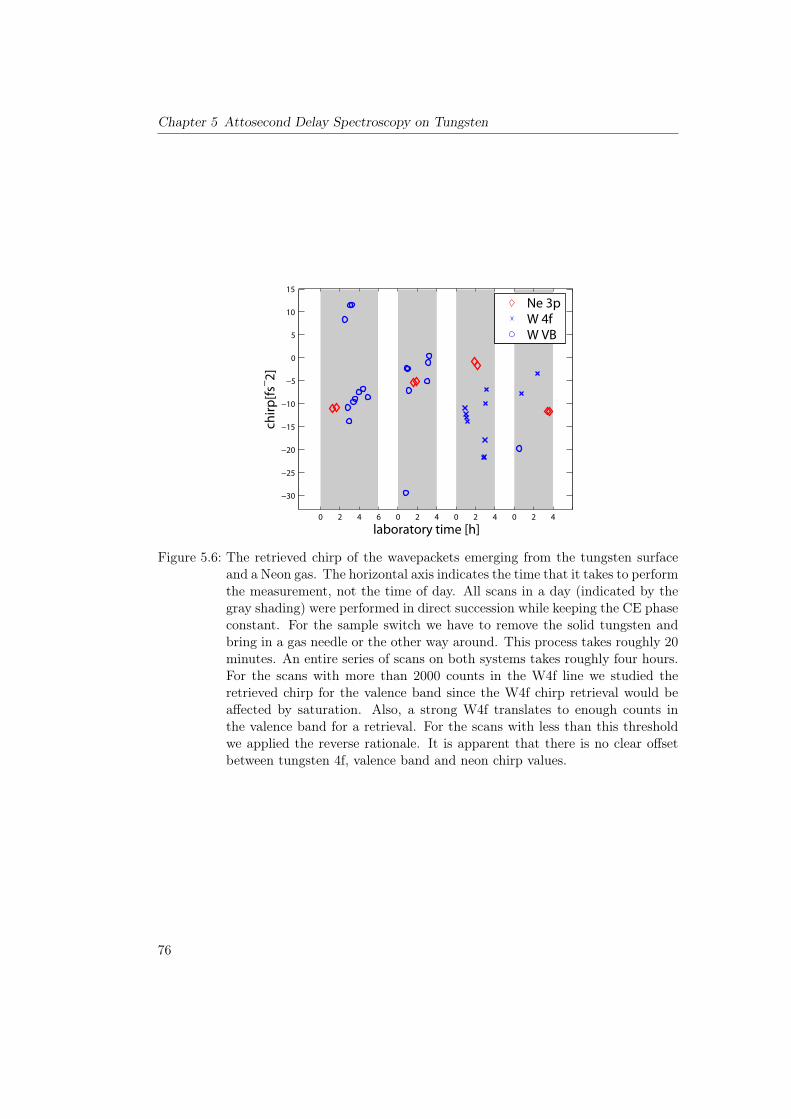
Chapter 5 Attosecond Delay Spectroscopy on Tungsten
!30
!25
!20
!15
!10
!5
0
5
10
15
laboratory time [h]
chirp
[fs! 2]
0 2 4 6 0 2 4 0 2 4 0 2 4
Ne 3pW 4fW VB
Figure 5.6: The retrieved chirp of the wavepackets emerging from the tungsten surfaceand a Neon gas. The horizontal axis indicates the time that it takes to performthe measurement, not the time of day. All scans in a day (indicated by thegray shading) were performed in direct succession while keeping the CE phaseconstant. For the sample switch we have to remove the solid tungsten andbring in a gas needle or the other way around. This process takes roughly 20minutes. An entire series of scans on both systems takes roughly four hours.For the scans with more than 2000 counts in the W4f line we studied theretrieved chirp for the valence band since the W4f chirp retrieval would beaffected by saturation. Also, a strong W4f translates to enough counts inthe valence band for a retrieval. For the scans with less than this thresholdwe applied the reverse rationale. It is apparent that there is no clear offsetbetween tungsten 4f, valence band and neon chirp values.
76

5.5 Delay Spectroscopy of Tungsten and O/W at a Photon Energy of 145eV
!100 !50 0 50 1000
5
10
15
delay [as]
# of
mea
sure
men
ts
All scans COELow chirp, no saturation COE
!100 !50 0 50 1000
5
10
15
delay [as]
# of
mea
sure
men
ts
All scans TDSELow chirp, no saturation TDSE
Figure 5.7: The dataset of all evaluated scans and the subset below the critical chirpabsolute value of 13 fs�2. The area graph represents a normal distributionwith the width and mean value of the corresponding data. The retrievedmean values for the delay in the respective subset and evaluation method areindicated as dashed lines. For all the subsets and evaluation methods theretrieved values are well within the error bars of all other subsets. A detaileddiscussion is given in 5.4.
between retrieved chirp and delay in the measured data. A trustworthy chirp retrievalin the 4f line is only possible for scans that are not saturated so we excluded scans withmore than 2000 counts in the W4f line. Among these data points we found that the scanswith a chirp absolute value smaller than 13 fs�2 showed no correlation between chirp anddelay. The mean delay value for this subset was (8± 24) as, which is within one third ofthe standard deviation from the value for all scans, (2± 35) as.As a further check on the performance of our retrieval we evaluated the data with thecenter of energy method and found very similar results. The histograms for all of the justmentioned subsets are shown in figure 5.7. The retrieved values for the just mentionedsubsets are:
Subset Delay Number of Scans
All scans (2± 35) as 132All scans, COE (6± 37) as 132No saturation (�2± 27) as 59Low chirp (10± 31) as 101Low chirp, no saturation (8± 24) as 38Low chirp, no saturation, COE (10± 29) as 38
77

Chapter 5 Attosecond Delay Spectroscopy on Tungsten
5.5.2 Clean Tungsten 100
We performed additional measurements on tungsten at a different crystal orientation.Gathering data on the same material means that we are probing a system with the samecross sections, escape depths and localization properties but a different band structure.The crystal is cleaned in a similar procedure as W(110) in UHV and the measurementperformed in the same way. The histogram of our delay findings is shown in figure 5.8.For these data there remains a weak correlation6 for all chirp values. When we arestudying only the spectrograms that are not saturated we are left with just 10 out of the40 performed scans, so the applicability of statistical terms becomes questionable. Wesaw that the COE results scattered heavily with a result of (42± 55) as, so we scrutinizedthe data with another method: the ATTOGRAM algorithm by Justin Gagnon [44, 125].This algorithm performs a full FROG retrieval of the spectrogram while assuming thatthere is just one state to be ionized. If it is applied to the tungsten data it will assumethat the XUV pulse consists of two spectrally separated pulses in order to reproducethe W4f and valence band line. Since this is a FROG retrieval it yields the phase ofthe XUV pulse. From this phase one can calculate the group delay – and the differencebetween the group delay in the W4f and VB line corresponds to the emission delay weare interested in. This analysis was first applied by Schultze et al. [19]. Here it wasperformed by Johann Riemensberger. The retrieved delay values for all methods are:
Subset Delay Number of Scans
All scans, TDSE (�13± 30) as 40All scans, COE (�17± 37) as 40All scans, Attogram (5± 24) as 36No Saturation (�17± 37) as 10
Four scans had to be excluded from the Attogram retrieval as the algorithm did notconverge. All methods and subsets yield results that are within one standard deviationof each other.
5.5.3 Measurements on O/W
As mentioned in the preceding sections a chirp retrieval for the valence band is a difficultendeavor due to the low signal strength. Increasing it would also mean saturation inthe 4f line, making an analysis of the chirp in the 4f line impossible – while still leavingthe valence band signal quite low for a reliable chirp retrieval. For the O/W system thesituation is different: the cross section of the valence band is now larger and allows for amore trustworthy analysis (see figure 5.9). On the other hand the retrieved chirp valueswould be more difficult to interpret since the valence band is now comprised of two atomicspecies. We thus focused our efforts on the delay measurement. We slightly saturated
6The probability that the observed distribution occurs by chance is roughly 20%. Usually one wouldspeak of a correlation if this probability is below 5%
78

5.5 Delay Spectroscopy of Tungsten and O/W at a Photon Energy of 145eV
!60 !40 !20 0 20 400
2
4
6
8
10
delay [as]
# o
f m
easu
rem
ents
All scansNo Saturation, Low chirp
Figure 5.8: A histogram of all acquired data on tungsten in the 100 orientation at 145 eVcompared to the selected scans that were not saturated and had less than15 fs�2 chirp. Note that the graph is not centered at zero but at the meanvalue of the unsaturated scans: (�17± 37) as
0 10 20 30 40 500
0.2
0.4
0.6
0.8
1
Binding Energy
Am
plit
ud
e [
a.u
.]
O(1x1)!W(110)
Figure 5.9: A static spectrum of oxygen on tungsten (110) acquired with a 145 eV mirrorwith a FWHM of 4.5 eV. Compared to the static spectrum for clean tungsten(see figure 5.5) it is apparent that the valence band region yields a muchstronger signal, as expected from the cross sections.
79
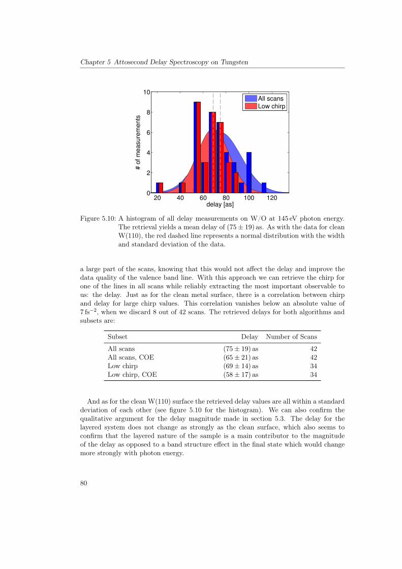
Chapter 5 Attosecond Delay Spectroscopy on Tungsten
20 40 60 80 100 1200
2
4
6
8
10
delay [as]
# o
f m
easu
rem
ents
All scansLow chirp
Figure 5.10: A histogram of all delay measurements on W/O at 145 eV photon energy.The retrieval yields a mean delay of (75± 19) as. As with the data for cleanW(110), the red dashed line represents a normal distribution with the widthand standard deviation of the data.
a large part of the scans, knowing that this would not affect the delay and improve thedata quality of the valence band line. With this approach we can retrieve the chirp forone of the lines in all scans while reliably extracting the most important observable tous: the delay. Just as for the clean metal surface, there is a correlation between chirpand delay for large chirp values. This correlation vanishes below an absolute value of7 fs�2, when we discard 8 out of 42 scans. The retrieved delays for both algorithms andsubsets are:
Subset Delay Number of Scans
All scans (75± 19) as 42All scans, COE (65± 21) as 42Low chirp (69± 14) as 34Low chirp, COE (58± 17) as 34
And as for the clean W(110) surface the retrieved delay values are all within a standarddeviation of each other (see figure 5.10 for the histogram). We can also confirm thequalitative argument for the delay magnitude made in section 5.3. The delay for thelayered system does not change as strongly as the clean surface, which also seems toconfirm that the layered nature of the sample is a main contributor to the magnitudeof the delay as opposed to a band structure effect in the final state which would changemore strongly with photon energy.
80

5.6 Overview of Delay Measurements on Tungsten
5.6 Overview of Delay Measurements on Tungsten
In figure 5.11 the results of all delay measurements on clean tungsten (110), tungsten(100), tungsten (110) with an oxygen adlayer and tungsten (110) with a hydrogen adlayerare shown. Comparing this graph to figure 5.2 emphasizes the new trend in the data.Before the measurements at high photon energies we had to presume an ongoing drop inthe delay for increasing XUV photon energies. But the new data points reveal a peculiarbehavior for clean tungsten. The delay change with increasing photon energy starts ata relatively flat slope of ⇡ 1 as
eV for the low energy side, then quadruples between 105 eVand 118 eV and then reverts back to the flat slope. With the additional data point athigher energies we can now see that there is not an ongoing drop increasing in steepnessbut actually a step in the delay. The data confirms that this is not only the case forthe (110) orientation but also for the (100) orientation of tungsten. The band structurediffers between these two crystal faces, but the localization, surface to bulk ratio andescape depth do not. This makes a band structure effect unlikely as a cause of the mea-sured delay. As mentioned in section 5.2 it is possible that the calculations emphasizingthe contrast between surface and bulk emission as the leading cause for the delay are notcontradicted by our findings on H/W. The experiments yielded a negligible differencebetween emission from tungsten 110 with and without a hydrogen adlayer at 105 eV.If the hydrogen merely rearranges the emission in the Brillouin zone towards larger k-vectors in the surface plane we would still observe surface states even if their emissionis strongly reduced in the direction perpendicularly to the surface. It is possible to testthis behavior with our setup by comparing scans that were obtained with and withoutthe electrostatic lens of the TOF detector. Without the lens the system has a collectionangle of ca. ±2�. This is increased tenfold to ca. ±20� while using the lens and changesthe angular characteristics of the recorded photoelectrons significantly.
5.7 Conclusions
We have shown that it is possible to extend the streaking method for photoemission delaymeasurements to photon energies of 145 eV with a laser system based on CPA stages anda hollow core fiber. The currently maximally achievable photon energy with enough fluxfor photoelectron experiments on solids is around 150 eV. It is likely that this energy willincrease as soon as the pulses are completely compressed to the sub 4 fs range that isalready the standard mode of operation for the laser system without the booster stage.Delay measurements between the 4f core and valence levels have been performed at thehighest photon energy possible so far. These measurements have revealed that the bandstructure is unlikely to be the origin of the delay. At the short mean free paths thatare typical for our experiments the photoelectrons originate from the first few layers ofthe solid, where they spend only around 100 as before being streaked. Our data couldpotentially be the first step towards experimentally identifying a lower bound for the timeit takes to establish a band structure in a solid. Another possible interpretation hinges
81

Chapter 5 Attosecond Delay Spectroscopy on Tungsten
90 100 110 120 130 140 150!50
0
50
100
Photon energy [eV]
CB
! 4
f d
ela
y [a
s]
clean W(110)clean W(100)O(1x1)!W(110)H(1x1)!W(110)
Figure 5.11: An overview of all the streaking measurements performed on tungsten attwo crystal orientations, oxygen on tungsten and hydrogen on tungsten atcentral XUV energies of 93 eV, 105 eV, 118 eV, 126 eV and 145 eV. Somepoints have been slightly offset for clarity. The measurement at 126 eV hassuch small error bars because there are only four data points in this set thatwere all performed on the same day. The intra-day variation is typicallysignificantly smaller than the inter-day fluctuation and we thus have to takethis particular data point with a grain of salt.
82

5.8 Outlook
on the fact that we are integrating over a large angular range with our detector. Thiscould smear out the band structure effects and lead to only very small delays that wouldbe smaller than the statistical spread of the data. The effect of angular integrationcan be measured by comparing delay scans that were obtained with and without theelectrostatic lens of the TOF detector. It can also be quantified by performing streakingmeasurements with the hemispherical detector, which has an angular resolution.We have observed a correlation between chirp and delay in our data for sufficiently largechirp values. For the analysis as it is being performed now we can rule out a systematicerror in the retrieval software as we were able to prove by means of simulated data. Alsowe were able to draw our conclusions about the delay from a subset of data that doesnot show this correlation. But there might be a physical origin of this behavior. Sabbar,Heuser, and Boge recently reported on a measurement comparing the photoemissiondelays of neon and argon with chirped XUV pulses [126]. In the presence of chirp inthe XUV there is a relation between the instantaneous frequency (i.e. photon energy)and the arrival time of the XUV photons. Since there is also a relation between theabsorption cross section and the photon energy the arrival time of specific frequenciesis being matched to the emission time. In their report Sabbar, Heuser, and Boge areworking close to a dominant spectral feature in argon that strongly modulates the crosssection. It varies by more than 80% over the relevant bandwidth, which translates toa large chirp induced delay shift of over 100 as. In our case the cross sections vary bymuch less – only 4% for the W4f and 14% for the valence band. We would expect amuch smaller effect that can be buried in the statistical noise for small chirp values. Asthe W4f cross section increases and the valence band decreases with photon energy anegative chirp would introduce a negative delay – meaning the W4f electrons would beperceived as arriving earlier in the streaking field than they actually are. This is thequalitative behavior we observe in the experiment. As an experimental proof for themagnitude of the effect we could introduce additional chirp to the pulse by employinga thicker metal filter or by using chirped XUV mirrors and then compare the obtaineddelays [73]. It is unlikely that the delay values measured at lower photon energies havebeen heavily affected by chirp since the typical XUV pulses for these energies were lessstrongly chirped than the ones we were using at 145 eV. We believe that the multilayerXUV mirror is responsible for the high XUV chirp. It was the first chromium/scandiummultilayer mirror that was used in attosecond experiments and it introduces significantunwanted second order dispersion [127].A manuscript reporting on the photon energy dependence of the photoemission delay isbeing prepared [128].
5.8 Outlook
Based on our experimental findings we are looking to perform the following experimentsin the near future:
• Full compression of the NIR pulse.
83

Chapter 5 Attosecond Delay Spectroscopy on Tungsten
• Delay measurements at photon energies below 100 eV where we can generate enoughXUV photons to obtain a very high signal. This allows us to compare data acquiredwith and without the electrostatic lens. Then we can reproduce the H/W data with-out the lens and clarify the rearrangement of valence band states in the Brillouinzone.
• Obtain Static spectra and possibly streaking measurements of H/W at low photonenergies with the hemispherical detector. This is more challenging than the previouspoint but it would provide more detailed insight.
• A delay measurement at 112 eV – in between the two data points that show thedrastic change in slope. With this experiment we can find out where the step reallyoccurs and how steep it is – or whether there is even a peak.
• Variation of the chirp of the XUV pulse with the help of filters to verify the influenceof chirp on the emission delay.
84
Bibliography
[1] M. Hentschel et al. “Attosecond metrology”. In: Nature 414.6863 (2001), pp. 509–513 (cit. on pp. 1, 4, 12, 23).
[2] A. Föhlisch et al. “Direct observation of electron dynamics in the attoseconddomain.” In: Nature 436.7049 (2005), pp. 373–6. doi: 10.1038/nature03833 (cit.on p. 1).
[3] T. Udem et al. “Accurate measurement of large optical frequency differences witha mode-locked laser”. In: Opt. Lett. 24.13 (1999), pp. 881–883. doi: 10.1364/OL.24.000881 (cit. on p. 2).
[4] T. Fuji et al. “Attosecond control of optical waveforms”. In: New J. Phys. 7 (2005),pp. 116–116. doi: 10.1088/1367-2630/7/1/116 (cit. on p. 2).
[5] P. Eckle et al. “Attosecond angular streaking”. In: Nat. Phys. 4.7 (2008), pp. 565–570. doi: 10.1038/nphys982 (cit. on p. 2).
[6] P. Eckle et al. “Attosecond ionization and tunneling delay time measurements inhelium.” In: Science 322.5907 (2008), pp. 1525–9. doi: 10.1126/science.1163439(cit. on p. 2).
[7] L. Torlina et al. “Interpreting Attoclock Measurements of Tunnelling Times”. In:ArXiv e-prints (2014). arXiv: 1402.5620 [physics.atom-ph] (cit. on p. 2).
[8] B. Bergues et al. “Attosecond tracing of correlated electron-emission in non-sequential double ionization.” In: Nat. Commun. 3.May (2012), p. 813. doi: 10.1038/ncomms1807 (cit. on p. 2).
[9] T. Wittmann et al. “Single-shot carrier–envelope phase measurement of few-cyclelaser pulses”. In: Nat. Phys. 5.5 (2009), pp. 357–362. doi: 10.1038/nphys1250(cit. on p. 2).
[10] A. Mcpherson et al. “Studies of multiphoton production of vacuum-ultravioletradiation in the rare gases”. In: J. Opt. Soc. Am. B 4.4 (1987), pp. 595–601 (cit.on pp. 2, 9).
[11] P. B. Corkum. “Plasma perspective on strong field multiphoton ionization”. In:Phys. Rev. Lett. 71.13 (1993), pp. 1994–1997. doi: 10.1103/PhysRevLett.71.1994 (cit. on pp. 2, 9, 10).
[12] J. Itatani et al. “Tomographic imaging of molecular orbitals”. In: Nature 432.7019(2004), pp. 867–871 (cit. on p. 2).
85

Bibliography
[13] N. L. Wagner et al. “Monitoring molecular dynamics using coherent electrons fromhigh harmonic generation”. In: Proc. Natl. Acad. Sci. 103.36 (2006), pp. 13279–13285. doi: 10.1073/pnas.0605178103 (cit. on p. 2).
[14] H. J. Wörner et al. “Following a chemical reaction using high-harmonic interfer-ometry.” In: Nature 466.7306 (2010), pp. 604–7. doi: 10.1038/nature09185 (cit.on p. 2).
[15] H. Dachraoui et al. “Photoinduced Reconfiguration Cycle in a Molecular Adsor-bate Layer Studied by Femtosecond Inner-Shell Photoelectron Spectroscopy”. In:Phys. Rev. Lett. 106.10 (2011), pp. 46–49. doi: 10.1103/PhysRevLett.106.107401 (cit. on pp. 3, 58, 64).
[16] K. Zhao et al. “Tailoring a 67 attosecond pulse through advantageous phase-mismatch”. In: Opt. Lett. 37.18 (2012), pp. 3891–3893. doi: 10.1364/OL.37.003891 (cit. on p. 3).
[17] E. Goulielmakis et al. “Real-time observation of valence electron motion”. In:Nature 466.7307 (2010), pp. 739–743 (cit. on p. 3).
[18] M. Schultze et al. “Controlling dielectrics with the electric field of light”. In: Nature493.7430 (2013), pp. 75–78 (cit. on p. 3).
[19] M. Schultze et al. “Delay in Photoemission”. In: Science 328.5986 (2010), pp. 1658–1662. doi: 10.1126/science.1189401 (cit. on pp. 4, 78).
[20] A. L. Cavalieri et al. “Attosecond spectroscopy in condensed matter.” In: Nature449.7165 (2007), pp. 1029–32. doi: 10.1038/nature06229 (cit. on pp. 4, 6, 14,65–69).
[21] W. A. Okell et al. “Attosecond streaking of photoelectron emission from disorderedsolids”. In: ArXiv e-prints (2014). arXiv: 1410.5613 [physics.optics] (cit. onp. 4).
[22] S. Neppl et al. “Direct observation of electron propagation and dielectric screeningon the atomic length scale”. In: Accept. Publ. Nat. (2014) (cit. on pp. 4, 25).
[23] J. H. Houtgraaf, J. Versmissen, and W. J. van der Giessen. “A concise review ofDNA damage checkpoints and repair in mammalian cells.” In: Cardiovasc. Revasc.Med. 7.3 (2006), pp. 165–72. doi: 10.1016/j.carrev.2006.02.002 (cit. on p. 5).
[24] J. C. Farman, B. G. Gardiner, and J. D. Shanklin. “Large losses of total ozone inAntarctica reveal seasonal ClOx/NOx interaction”. In: Nature 315 (1985), pp. 207–210. doi: 10.1038/315207a0 (cit. on p. 5).
[25] A. Jones and J. Shanklin. “Continued decline of total ozone over Halley, Antarc-tica, since 1985”. In: Nature 376.6539 (1995), pp. 409–411 (cit. on p. 5).
[26] Y. Matsumi and M. Kawasaki. “Photolysis of atmospheric ozone in the ultravioletregion.” In: Chem. Rev. 103.12 (2003), pp. 4767–82. doi: 10.1021/cr0205255(cit. on p. 5).
86

Bibliography
[27] G. J. Halász et al. “Simulation of laser-induced quantum dynamics of the electronicand nuclear motion in the ozone molecule on the attosecond time scale”. In: Phys.Rev. A 86.4 (2012), p. 043426. doi: 10.1103/PhysRevA.86.043426 (cit. on pp. 5,41, 44).
[28] B. Mignolet, R. D. Levine, and F. Remacle. “Localized electron dynamics inattosecond-pulse-excited molecular systems: Probing the time-dependent electrondensity by sudden photoionization”. In: Phys. Rev. A 86.5 (2012), p. 053429. doi:10.1103/PhysRevA.86.053429 (cit. on p. 5).
[29] F. Remacle and R. D. Levine. “An electronic time scale in chemistry”. In: Proc.Natl. Acad. Sci. U. S. A. 103.18 (2006), pp. 6793–6798. doi: 10.1073/pnas.0601855103 (cit. on p. 5).
[30] M. Grätzel. “Dye-sensitized solar cells”. In: J. Photochem. Photobiol. C Pho-tochem. Rev. 4.2 (2003), pp. 145–153. doi: 10.1016/S1389-5567(03)00026-1(cit. on pp. 5, 51).
[31] B. Oregan and M. Gratzel. “A Low-cost, High-efficiency Solar-cell Based On Dye-sensitized Colloidal Tio2 Films”. In: Nature 353.6346 (1991), pp. 737–740 (cit. onp. 5).
[32] J. Schnadt et al. “Experimental evidence for sub-3-fs charge transfer from anaromatic adsorbate to a semiconductor”. In: Nature 418 (2002), pp. 620–623 (cit.on p. 5).
[33] R. W. Boyd. Nonlinear Optics. 3rd editio. Academic Press Inc, 2003 (cit. on pp. 8,9, 15).
[34] K. Kulander, K. Schafer, and J. Krause. “Dynamics of short-pulse excitation,ionization and harmonic conversion”. In: Super-Intense Laser-Atom Phys. Ed. byB. Piraux, A. L’huillier, and K. Rzazewski. Vol. 316. New York: Plenum, 1993,p. 95 (cit. on p. 9).
[35] K. J. Schafer et al. “Above threshold ionization beyond the high harmonic cutoff”.In: Phys. Rev. Lett. 70.11 (1993), pp. 1599–1602. doi: 10.1103/PhysRevLett.70.1599 (cit. on p. 9).
[36] M. Lewenstein et al. “Theory of high-harmonic generation by low-frequency laserfields”. In: Phys. Rev. A 49.3 (1994), pp. 2117–2132. doi: 10.1103/PhysRevA.49.2117 (cit. on p. 9).
[37] K. Varjú et al. “Physics of attosecond pulses produced via high harmonic gener-ation”. In: Am. J. Phys. 77.5 (2009), p. 389. doi: 10.1119/1.3086028 (cit. onpp. 10, 11).
[38] G. Sansone et al. “Isolated single-cycle attosecond pulses.” In: Science (80-. ).314.5798 (2006), pp. 443–6. doi: 10.1126/science.1132838 (cit. on p. 10).
[39] P. Heissler et al. “Few-Cycle Driven Relativistically Oscillating Plasma Mirrors: ASource of Intense Isolated Attosecond Pulses”. In: Phys. Rev. Lett. 108.23 (2012),p. 235003. doi: 10.1103/PhysRevLett.108.235003 (cit. on p. 10).
87

Bibliography
[40] T. W. Barbee , Jr., S. Mrowka, and M. C. Hettrick. “Molybdenum-silicon multi-layer mirrors for the extreme ultraviolet”. In: Appl. Opt. 24.6 (1985), p. 883. doi:10.1364/AO.24.000883 (cit. on p. 10).
[41] M. Hofstetter et al. “Lanthanum-molybdenum multilayer mirrors for attosecondpulses between 80 and 130 eV”. In: New J. Phys. 13.6 (2011), p. 063038. doi:10.1088/1367-2630/13/6/063038 (cit. on p. 10).
[42] V. S. Yakovlev, F. Bammer, and A. Scrinzi. “Attosecond streaking measurements”.In: J. Mod. Opt. 52.2-3 (2005), pp. 395–410. doi: 10.1080/09500340412331283642(cit. on p. 11).
[43] F. Krausz and M. Ivanov. “Attosecond physics”. In: Rev. Mod. Phys. 81.1 (2009),pp. 163–234. doi: 10.1103/RevModPhys.81.163 (cit. on p. 11).
[44] J. Gagnon. “Attosecond electron spectroscopy theory and its applications”. PhDthesis. Ludwig-Maximilians-Universität München, 2010 (cit. on pp. 11, 78).
[45] D. J. Bradley, B. Liddy, and W. E. Sleat. “Direct linear measurement of ultra-short light pulses with a picosecond streak camera”. In: Opt. Commun. 2.8 (1971),pp. 391–395. doi: http://dx.doi.org/10.1016/0030-4018(71)90252-5 (cit. onp. 11).
[46] E. Goulielmakis et al. “Direct measurement of light waves.” In: Science 305.5688(2004), pp. 1267–9. doi: 10.1126/science.1100866 (cit. on p. 13).
[47] R. Kienberger et al. “Atomic transient recorder”. In: Nature 427.6977 (2004),pp. 817–821 (cit. on p. 14).
[48] V. S. Yakovlev et al. “Attosecond Streaking Enables the Measurement of QuantumPhase”. In: Phys. Rev. Lett. 105.7 (2010), p. 073001. doi: 10.1103/PhysRevLett.105.073001 (cit. on p. 14).
[49] M. T. Ossiander. “On the Expansion of Attosecond Streaking Spectroscopy to-wards Ultrafast Surface Dynamics”. MA thesis. Technische Universität München,2014 (cit. on p. 14).
[50] P. Baum, S. Lochbrunner, and E. Riedle. “Generation of tunable 7-fs ultravioletpulses: achromatic phase matching and chirp management”. In: Appl. Phys. B79.8 (2004), pp. 1027–1032. doi: 10.1007/s00340-004-1668-2 (cit. on p. 15).
[51] P. Baum, S. Lochbrunner, and E. Riedle. “Tunable sub-10-fs ultraviolet pulses gen-erated by achromatic frequency doubling.” In: Opt. Lett. 29.14 (2004), pp. 1686–8(cit. on p. 15).
[52] F. Reiter et al. “Generation of sub-3 fs pulses in the deep ultraviolet.” In: Opt.Lett. 35.13 (2010), pp. 2248–50 (cit. on pp. 15, 36, 39, 50).
[53] R. Trebino. Frequency-Resolved Optical Gating: The Measurement of UltrashortLaser Pulses. Boston, MA: Springer US, 2000. doi: 10.1007/978-1-4615-1181-6(cit. on p. 16).
88

Bibliography
[54] R. Trebino et al. “Measuring ultrashort laser pulses in the time-frequency do-main using frequency-resolved optical gating”. In: Rev. Sci. Instrum. 68.9 (1997),p. 3277. doi: 10.1063/1.1148286 (cit. on p. 16).
[55] J. N. Sweetser, D. N. Fittinghoff, and R. Trebino. “Transient-grating frequency-resolved optical gating.” In: Opt. Lett. 22.8 (1997), pp. 519–21 (cit. on p. 16).
[56] H. W. Schweinberger. “A Laser Source for the Generation of Intense AttosecondPulses and its First Applications”. PhD thesis. Ludwig-Maximilians-UniversitätMünchen, 2014 (cit. on p. 17).
[57] R. Szipocs et al. “Chirped multilayer coatings for broadband dispersion control infemtosecond lasers.” In: Opt. Lett. 19.3 (1994), p. 201 (cit. on p. 17).
[58] A. Stingl et al. “Sub-10-fs mirror-dispersion-controlled Ti:sapphire laser.” In: Opt.Lett. 20.6 (1995), pp. 602–4 (cit. on p. 17).
[59] T. Fuji et al. “Monolithic carrier-envelope phase-stabilization scheme.” In: Opt.Lett. 30.3 (2005), pp. 332–4 (cit. on p. 17).
[60] D. Strickland and G. Mourou. “Compression of amplified chirped optical pulses”.In: Opt. Commun. 55.6 (1985), pp. 447–449 (cit. on p. 17).
[61] P. Tournois. “Acousto-optic programmable dispersive filter for adaptive compen-sation of group delay time dispersion in laser systems”. In: Opt. Commun. 4018.Au-gust (1997) (cit. on p. 17).
[62] T. Clausnitzer et al. “Highly efficient transmission gratings in fused silica forchirped-pulse amplification systems”. In: Appl. Opt. 42.34 (2003), pp. 6934–6938.doi: 10.1364/AO.42.006934 (cit. on p. 21).
[63] J. Rauschenberger et al. “Carrier-envelope phase-stabilized amplifier system”. In:Laser Phys. Lett. 3.1 (2006), pp. 37–42. doi: 10.1002/lapl.200510053 (cit. onp. 21).
[64] A. Baltuska et al. “Phase-controlled amplification of few-cycle laser pulses”. In:Sel. Top. Quantum Electron. IEEE J. 9.4 (2003), pp. 972–989. doi: 10.1109/JSTQE.2003.819107 (cit. on p. 21).
[65] A. L. Cavalieri et al. “Intense 1.5-cycle near infrared laser waveforms and theiruse for the generation of ultra-broadband soft-x-ray harmonic continua”. In: NewJ. Phys. 9.7 (2007), p. 242 (cit. on pp. 22, 57).
[66] P. O’shea et al. “Increased-bandwidth in ultrashort-pulse measurement using anangle-dithered nonlinear-optical crystal”. In: Opt. Express 7.10 (2000), p. 342. doi:10.1364/OE.7.000342 (cit. on p. 22).
[67] Patrick Rupprecht. “FROG / 2DSI dual Characterization of Femtosecond Pulsesusing External Dithering”. BA thesis. Technische Universität München, 2014 (cit.on p. 23).
[68] E. Magerl et al. “A flexible apparatus for attosecond photoelectron spectroscopyof solids and surfaces”. In: Rev. Sci. Instrum. 82.6 (2011), p. 063104. doi: 10.1063/1.3596564 (cit. on pp. 23, 26).
89

Bibliography
[69] S. Neppl. “Attosecond Time-Resolved Photoemission from Surfaces and Inter-faces”. PhD thesis. Technische Universität München, 2012 (cit. on pp. 25, 26, 67–71, 74, 75).
[70] S. Hüfner. Photoelectron spectroscopy: principles and applications. Springer Verlag,2003 (cit. on pp. 25, 55).
[71] A. Naumkin et al. NIST XPS Database. 2012 (cit. on pp. 26, 56).[72] K. Varju, P. Johnsson, and R. Lopez-martens. “Experimental studies of attosecond
pulse trains”. In: Laser Phys. 15.6 (2005), pp. 888–898 (cit. on p. 26).[73] M. Hofstetter et al. “Attosecond dispersion control by extreme ultraviolet multi-
layer mirrors.” In: Opt. Express 19.3 (2011), pp. 1767–76 (cit. on pp. 26, 83).[74] S. Neppl et al. “Attosecond Time-Resolved Photoemission from Core and Valence
States of Magnesium”. In: Phys. Rev. Lett. 109.8 (2012), p. 087401. doi: 10.1103/PhysRevLett.109.087401 (cit. on p. 26).
[75] M. Fiess et al. “Versatile apparatus for attosecond metrology and spectroscopy”.In: Rev. Sci. Instrum. 81.9 (2010), p. 93103. doi: 10.1063/1.3475689 (cit. onp. 27).
[76] C. Jakubeit. “Upgrade of an Attosecond Beamline”. MA thesis. Technische Uni-versität München, 2013 (cit. on pp. 27, 28).
[77] A. Serdyuchenko et al. “High spectral resolution ozone absorption cross-sections– Part 2: Temperature dependence”. In: Atmos. Meas. Tech. 7.2 (2014), pp. 625–636. doi: 10.5194/amt-7-625-2014 (cit. on p. 30).
[78] H. Keller-rudek et al. “The MPI-Mainz UV/VIS Spectral Atlas of Gaseous Moleculesof Atmospheric Interest”. In: Earth Syst. Sci. Data 5.2 (2013), pp. 365–373. doi:10.5194/essd-5-365-2013 (cit. on p. 30).
[79] S. Sander et al. “Chemical Kinetics and Photochemical Data for Use in Atmo-spheric Studies. Evaluation Number 15”. In: JPL Publ. 06-2 (2006) (cit. on p. 30).
[80] G. M. Platz and C. K. Hersh. “Preparation of Liquid Ozone and Ozone-OxygenMixtures for Rocket Application”. In: Ind. Eng. Chem. 48.4 (1956), pp. 742–744.doi: 10.1021/ie50556a024 (cit. on p. 31).
[81] G. A. Cook et al. “Explosion Limits of Ozone-oxygen Mixtures”. In: Ind. Eng.Chem. 48.4 (1956), pp. 736–741 (cit. on p. 31).
[82] H. von Siemens. “Über Dampfdruckmessungen und Thermometrie bei tiefen Tem-peraturen”. In: Ann. Phys. 42.14 (1913), 871–U40 (cit. on p. 31).
[83] D. Hanson and K. Mauersberger. “The Vapor-pressures of Solid and Liquid Ozone”.In: J. Chem. Phys. 85.8 (1986), pp. 4669–4672 (cit. on p. 31).
[84] E. Coleman et al. “A Versatile Low-pressure Ozone Source”. In: J. Vac. Sci. Tech-nol. A 9.4 (1991), pp. 2408–2409 (cit. on p. 31).
[85] U. Graf et al. “Intense few-cycle light pulses in the deep ultraviolet”. In: Opt.Express 16.23 (2008), pp. 18956–18963 (cit. on pp. 32, 36, 39, 50).
90
Bibliography
[86] T. Metzger et al. “High-repetition-rate picosecond pump laser based on a Yb:YAGdisk amplifier for optical parametric amplification”. In: Opt. Lett. 34.14 (2009),pp. 2123–2125. doi: 10.1364/OL.34.002123 (cit. on p. 33).
[87] S. Kahra et al. “A molecular conveyor belt by controlled delivery of single moleculesinto ultrashort laser pulses”. In: Nat. Phys. 8.3 (2012), pp. 238–242. doi: 10.1038/nphys2214 (cit. on p. 39).
[88] A. Schiffrin et al. “Optical-field-induced current in dielectrics.” In: Nature 493.7430(2013), pp. 70–4. doi: 10.1038/nature11567 (cit. on p. 40).
[89] S. Y. Grebenshchikov et al. “New theoretical investigations of the photodissoci-ation of ozone in the Hartley, Huggins, Chappuis, and Wulf bands”. In: Phys.Chem. Chem. Phys. 9.17 (2007), pp. 2044–2064. doi: 10.1039/b701020f (cit. onp. 40).
[90] G. J. Halász et al. “Coherence revival during the attosecond electronic and nuclearquantum photodynamics of the ozone molecule”. In: Phys. Rev. A 88.2 (2013),p. 023425. doi: 10.1103/PhysRevA.88.023425 (cit. on pp. 41, 43).
[91] D. Imre et al. “Chemical dynamics studied by emission spectroscopy of dissociat-ing molecules”. In: J. Phys. Chem. 88.18 (1984), pp. 3956–3964. doi: 10.1021/j150662a017 (cit. on p. 42).
[92] A. Perveaux et al. “Attosecond electronic and nuclear quantum photodynamics ofozone: time-dependent Dyson orbitals and dipole”. In: J. Phys. B At. Mol. Opt.Phys. 47.12 (2014), p. 124010. doi: 10.1088/0953-4075/47/12/124010 (cit. onp. 42).
[93] L. Grill and C. Joachim. Imaging and Manipulating Molecular Orbitals. Septem-ber. Springer Berlin Heidelberg, 2013. doi: http://dx.doi.org/10.1007/978-3-642-38809-5?nosfx=yVerlagVolltext (cit. on pp. 42, 54).
[94] A. Perveaux et al. “Monitoring the Birth of an Electronic Wavepacket in a Moleculewith Attosecond Time-Resolved Photoelectron Spectroscopy”. In: J. Phys. Chem.A 118.38 (2014), pp. 8773–8778. doi: 10.1021/jp508218n (cit. on pp. 42, 43).
[95] T. Latka. Private Communications (cit. on p. 44).[96] F. Schwabl. Quantenmechanik. Springer Verlag, 2008 (cit. on p. 44).[97] D. Kuciauskas et al. “Transient Absorption Spectroscopy of Ruthenium and Os-
mium Polypyridyl Complexes Adsorbed onto Nanocrystalline TiO2 Photoelec-trodes”. In: J. Phys. Chem. B 106.36 (2002), pp. 9347–9358 (cit. on p. 51).
[98] G. Sauve et al. “Dye sensitization of nanocrystalline titanium dioxide with os-mium and ruthenium polypyridyl complexes”. In: J. Phys. Chem. B 104.29 (2000),pp. 6821–6836. doi: 10.1021/jp0002143 (cit. on pp. 52, 54).
[99] S. Tanuma, C. J. Powell, and D. R. Penn. “Calculations of electron inelastic meanfree paths. IX. Data for 41 elemental solids over the 50 eV to 30 keV range”. In:Surf. Interface Anal. 43.3 (2011), pp. 689–713. doi: 10.1002/sia.3522 (cit. onpp. 53, 68).
91

Bibliography
[100] A. Schiffrin. Private Communications. 2012 (cit. on p. 54).[101] J. Yeh and I. Lindau. “Atomic subshell photoionization cross sections and asym-
metry parameters”. In: At. data Nucl. data tables 32.l (1985) (cit. on pp. 54, 70).[102] Atomic Calculation of Photoionization Cross-Sections and Asymmetry Parameters
(cit. on pp. 54, 70).[103] J. V. Barth. “Molecular architectonic on metal surfaces.” In: Annu. Rev. Phys.
Chem. 58 (2007), pp. 375–407. doi: 10.1146/annurev.physchem.56.092503.141259 (cit. on p. 54).
[104] H. Dürr and H. Bouas-laurent. Photochromism: Molecules and Systems. ElsevierScience, 2003 (cit. on p. 54).
[105] T. A. Heimer, C. A. Bignozzi, and G. J. Meyer. “Molecular-level Photovoltaics -the Electrooptical Properties of Metal Cyanide Complexes Anchored To Titanium-dioxide”. In: J. Phys. Chem. 97.46 (1993), pp. 11987–11994 (cit. on p. 54).
[106] K.-L. Wu et al. “Engineering of osmium(II)-based light absorbers for dye-sensitizedsolar cells.” In: Angew. Chem. Int. Ed. Engl. 51.23 (2012), pp. 5642–6. doi: 10.1002/anie.201200071 (cit. on p. 54).
[107] M. Majewski and M. Wolf. Private Communications. 2012 (cit. on p. 58).[108] F. Evangelista et al. “Electronic structure of copper phthalocyanine: an experi-
mental and theoretical study of occupied and unoccupied levels.” In: J. Chem.Phys. 126.12 (2007), p. 124709. doi: 10.1063/1.2712435 (cit. on pp. 61, 62).
[109] M. El-nahass et al. “Structural and optical properties of thermal evaporated mag-nesium phthalocyanine (MgPc) thin films”. In: Appl. Surf. Sci. 254.8 (2008),pp. 2458–2465. doi: 10.1016/j.apsusc.2007.09.064 (cit. on p. 61).
[110] G. Binnig et al. “Surface studies by scanning tunneling microscopy”. In: Phys.Rev. Lett. 49.1 (1982) (cit. on p. 61).
[111] J. F. Horstbrink. “Zeitaufgelöste spektroskopische Untersuchung ultraschnellerMoleküldynamik”. MA thesis. Technische Universität München, 2014 (cit. on p. 62).
[112] M. Gerl. “Time-resolved investigation of photoelectron dynamics by AttosecondStreaking Spectroscopy on solids”. MA thesis. Technische Universität München,2013 (cit. on pp. 67, 69).
[113] C.-H. Zhang and U. Thumm. “Attosecond Photoelectron Spectroscopy of MetalSurfaces”. In: Phys. Rev. Lett. 102.12 (2009), p. 123601. doi: 10.1103/PhysRevLett.102.123601 (cit. on pp. 67, 68).
[114] C. Lemell et al. “Simulation of attosecond streaking of electrons emitted froma tungsten surface”. In: Phys. Rev. A 79.6 (2009), p. 062901. doi: 10.1103/PhysRevA.79.062901 (cit. on pp. 67, 68).
[115] A. Kazansky and P. Echenique. “One-Electron Model for the Electronic Responseof Metal Surfaces to Subfemtosecond Photoexcitation”. In: Phys. Rev. Lett. 102.17(2009), p. 177401. doi: 10.1103/PhysRevLett.102.177401 (cit. on pp. 67, 68).
92
Bibliography
[116] E. E. Krasovskii. “Attosecond spectroscopy of solids: Streaking phase shift dueto lattice scattering”. In: Phys. Rev. B 84.19 (2011), p. 195106. doi: 10.1103/PhysRevB.84.195106 (cit. on pp. 68, 69).
[117] C. H. Zhang and U. Thumm. “Effect of wave-function localization on the timedelay in photoemission from surfaces”. In: Phys. Rev. A - At. Mol. Opt. Phys. 84(2011). doi: 10.1103/PhysRevA.84.065403 (cit. on p. 68).
[118] A. Borisov et al. “Resonant and nonresonant processes in attosecond streakingfrom metals”. In: Phys. Rev. B 87.12 (2013), p. 121110. doi: 10.1103/PhysRevB.87.121110 (cit. on pp. 68, 69).
[119] R. Bartynski et al. “Angle-resolved photoemission study of the surface and bulkelectronic structure of Mg (0001) and Mg (112- 0)”. In: Phys. Rev. B 33.6 (1986)(cit. on p. 68).
[120] F. Schiller et al. “Electronic structure of Mg: From monolayers to bulk”. In: Phys.Rev. B 70.12 (2004), p. 125106. doi: 10.1103/PhysRevB.70.125106 (cit. onp. 68).
[121] B. Feuerbacher and B. Fitton. “Electronic energy levels of hydrogen adsorbed ontungsten”. In: Phys. Rev. B 8.10 (1973) (cit. on p. 69).
[122] E. Rotenberg and S. Kevan. “Evolution of Fermi level crossings versus H coverageon W (110)”. In: Phys. Rev. Lett. (1998), pp. 2905–2908 (cit. on p. 69).
[123] A. Kim. “TBD”. PhD thesis. Technische Universität München, 2014 (cit. on pp. 70,75).
[124] M. Stöhr. “First Principles Investigations of Adsorption on a Transition MetalSurface: Oxygen and Indium on the (110) Surface of Tungsten”. PhD thesis. Uni-versität Wien, 2009 (cit. on p. 71).
[125] J. Gagnon, E. Goulielmakis, and V. Yakovlev. “The accurate FROG characteri-zation of attosecond pulses from streaking measurements”. In: Appl. Phys. B 92.1(2008), pp. 25–32. doi: 10.1007/s00340-008-3063-x (cit. on p. 78).
[126] M. Sabbar, S. Heuser, and R. Boge. “Attochirp-corrected photo ionization timedelays using coincidence attosecond streaking”. In: arXiv (2014) (cit. on p. 83).
[127] A. Guggenmos et al. “Ion polished Cr/Sc attosecond multilayer mirrors for highwater window reflectivity”. In: Opt. Express 22.22 (2014), p. 26526. doi: 10.1364/OE.22.026526 (cit. on p. 83).
[128] M. Jobst et al. “Excitation energy dependent photoemission timing in tungsten”.In: Prep. (2015) (cit. on p. 83).
93

Curriculum Vitae
Michael Jobstborn on August 2nd,1982
Education
04/2010—12/2014 PhD student at the Max Planck Institut for Quantum Op-tics in the group of Prof. Dr. Reinhard Kienberger andthe department of Prof. Dr. Krausz
08/2008—08/2009 Diploma thesis at ETH Zürich under supervision of Prof.Dr. Vahid Sandoghdar
08/2006—06/2007 Studies of physics at the University of Colorado at Boulder,USA
09/2003—08/2009 Studies of physics at the Universität Regensburg2002 Abitur at Gymnasium Neutraubling
Teaching
2012–2014 Advanced laboratory course, TU München2008–2009 Teaching assistant for several lectures, ETH Zürich
Publication List
P1 S. Neppl, R. Ernstorfer, A. L. Cavalieri, C. Lemell, G. Wachter, E. Magerl, E.Bothschafter, M. Jobst, M. Hofstetter, U. Kleineberg, J. Barth, D. Menzel,J. Burgdörfer, P. Feulner, F. Krausz, and R. Kienberger. “Direct observationof electron propagation and dielectric screening on the atomic length scale”.Accepted for publication in Nature (2014).
P2 M. Jobst, S. Neppl, E. Bothschafter, J. Riemensberger, M. Ossiander, M.Schäffer, E. Magerl, A. Kim, P. Feulner, and R. Kienberger. “Excitation energydependent photoemission timing in tungsten. In preparation (2015).
95

Bibliography
PresentationsO1 M. Jobst, M. Fieß, A. Sommer, S. Holzner, M. Schultze, F. Krausz and R.
Kienberger., “Towards time resolving attosecond electron dynamics in ozone”.ATTOFEL Summer School in Crete (2011)
O2 M. Jobst, S. Neppl, E. Bothschafter, W. Helml, A. Schiffrin, R. Ernstorfer, F.Krausz, and R. Kienberger. “Attosecond spectroscopy on solid surfaces (PosterPresentation)”. ATTOFEL Meeting in Berlin (2011)
O3 M. Jobst, M. Fieß, A. Sommer, S. Holzner, M. Schultze, F. Krausz, and R.Kienberger. “Towards time resolving attosecond electron dynamics in ozone”.FEMTO10 – The Madrid Conference on Femtochemistry, Poster Presentation(2011)
O4 M. Jobst, J. Riemensberger, M. Ossiander, M. Schäffer, S. Neppl, A.Kim,A.Guggenmoos, J.V. Barth, F. Krausz, P. Feulner, and R. Kienberger.“Photon-energy Dependent Delays in Photoemission from Tungsten Surfaces”.MAP-B Symposium (2014)
O5 M. Jobst. “Attosecond Dynamics in Molecules and on Interfaces”. Multipleoral contributions to the International Max Planck Research School of AdvancedPhoton Science
96
Chapter 6
Acknowledgement
First and foremost I would like to thank my Doktorvater Reinhard Kienberger for givingme the opportunity to perform cutting edge research while not forgetting that there ismore to life. Following the credo non scholae sed vitae discimus, I learned valuable lifeskills from him. He showed me when patience is necessary – not in the laboratory butalso when you have to tap a keg or properly fire up a small grill for feeding thirty people.I would like to thank Ferenc Krausz for providing the funding and laboratory environ-ment that make attosecond science possible. Working under the excellent conditionsprovided in his world leading group was a fascinating experience.I am sincerely grateful to Tobias Latka for powering through some tough pumplaser-lesstimes with me. He never lost patience when he had to align the laser as my colorblindnessprevented me from seeing the amplifier mode. In his case I can even overlook the factthat he is a BVB supporter!During my PhD studies I had the pleasure of supervising Clemens Jakubeit, Vahe Shir-vanyan and Patrick Rupprecht. I learned at least as much from them as they did fromme – thanks for the great working atmosphere. Patrick always kept me and our bankaccount on our respective toes. Clemens massively improved the music in the lab. Anda special shoutout goes to Vahe for keeping a tight check on Munich’s nocturnal X6population.Agustin Schiffrin was first a supervisor and then a collaboration partner – but he wasalways helpful, creative and humorous.My thanks also to the colleagues who were part of the long doodle-managed AS2 beam-time shifts: Elisabeth Bothschafter, Annkatrin Sommer, Martin Schultze and Wolfgangmagic fingers Schweinberger. Together we proved that we actually can organize our re-search in a way that includes long nights and weekends but still lets life inside and outsidethe laboratory coexist. The same holds true for AS3 with Johann Riemensberger, Mar-cus Ossiander and Wolfram Helml. The collaboration with Marcus on the unexpectedlyfruitful graphite experiment was particularly enjoyable. All of these colleagues madesure that we never had a boring lunch break. Even during the gloomiest chiller-infusednightmare we would all laugh together at IPP and then tackle the problems in the labwith renewed vigor.Hanieh Fattahi and Ayman Akil educated me about life in Iran and Lebanon – again Ilearned a life lesson about the small things we tend to take for granted.None of the attosecond experiments would have been possible without our mirror mak-ers. Olga Razskazovskaya and Alexander Guggenmos provided unconventional optics in
97
Chapter 6 Acknowledgement
record speed. When Alex promised a mirror in two weeks you would get it in two days.Special thanks to Nicholas Karpowicz for always being approachable with any question.I am convinced that it is impossible to have a five minute conversation with Nick withoutbecoming smarter in the process.Everyone in my office was incredibly relieved when it was confirmed that Peter Feulnerwould continue working after his 65th birthday. His unmatched laboratory experience issimply irreplaceable and was tremendously helpful.Miss Wild and her general unstoppability guaranteed that Frauenchiemsee and everyIMPRS event was flawlessly organized. I am sure she would be capable of herding catswithout breaking a sweat.I am grateful to the mechanical workshop of MPQ for dealing with my small requestsspontaneously – and with my large requests in time.My deepest gratitude goes to my parents for always supporting me.And last but definitely not least: thank you, Katharina. For everything.
98