Attractor Network Dynamics Enable Preplay andRapid Path Planning in Maze–like Environments

Dane CorneilLaboratory of Computational NeuroscienceEcole Polytechnique Federale de Lausanne

CH-1015 Lausanne, Switzerlanddane.corneil@epfl.ch

Wulfram GerstnerLaboratory of Computational NeuroscienceEcole Polytechnique Federale de Lausanne

CH-1015 Lausanne, Switzerlandwulfram.gerstner@epfl.ch

Abstract

Rodents navigating in a well–known environment can rapidly learn and revisit ob-served reward locations, often after a single trial. While the mechanism for rapidpath planning is unknown, the CA3 region in the hippocampus plays an importantrole, and emerging evidence suggests that place cell activity during hippocam-pal “preplay” periods may trace out future goal–directed trajectories. Here, weshow how a particular mapping of space allows for the immediate generation oftrajectories between arbitrary start and goal locations in an environment, basedonly on the mapped representation of the goal. We show that this representationcan be implemented in a neural attractor network model, resulting in bump–likeactivity profiles resembling those of the CA3 region of hippocampus. Neuronstend to locally excite neurons with similar place field centers, while inhibitingother neurons with distant place field centers, such that stable bumps of activitycan form at arbitrary locations in the environment. The network is initialized torepresent a point in the environment, then weakly stimulated with an input cor-responding to an arbitrary goal location. We show that the resulting activity canbe interpreted as a gradient ascent on the value function induced by a reward atthe goal location. Indeed, in networks with large place fields, we show that thenetwork properties cause the bump to move smoothly from its initial location tothe goal, around obstacles or walls. Our results illustrate that an attractor networkwith hippocampal–like attributes may be important for rapid path planning.

1 Introduction

While early human case studies revealed the importance of the hippocampus in episodic memory [1,2], the discovery of “place cells” in rats [3] established its role for spatial representation. Recentresults have further suggested that, along with these functions, the hippocampus is involved in activespatial planning: experiments in “one–shot learning” have revealed the critical role of the CA3region [4, 5] and the intermediate hippocampus [6] in returning to goal locations that the animal hasseen only once. This poses the question of whether and how hippocampal dynamics could supporta representation of the current location, a representation of a goal, and the relation between the two.

In this article, we propose that a model of CA3 as a “bump attractor” [7] can be be used for pathplanning. The attractor map represents not only locations within the environment, but also the spatialrelationship between locations. In particular, broad activity profiles (like those found in intermediateand ventral hippocampus [8]) can be viewed as a condensed map of a particular environment. Theplanned path presents as rapid sequential activity from the current position to the goal location,similar to the “preplay” observed experimentally in hippocampal activity during navigation tasks [9,10], including paths that require navigating around obstacles. In the model, the activity is producedby supplying input to the network consistent with the sensory input that would be provided at the

1

goal site. Unlike other recent models of rapid goal learning and path planning [11, 12], there isno backwards diffusion of a value signal from the goal to the current state during the learning orplanning process. Instead, the sequential activity results from the representation of space in theattractor network, even in the presence of obstacles.

The recurrent structure in our model is derived from the “successor representation” [13], whichrepresents space according to the number and length of paths connecting different locations. Theresulting network can be interpreted as an attractor manifold in a low–dimensional space, where thedimensions correspond to weighted version of the most relevant eigenvectors of the environment’stransition matrix. Such low–frequency functions have recently found support as a viable basis forplace cell activity [14–16]. We show that, when the attractor network operates in this basis and isstimulated with a goal location, the network activity traces out a path to that goal. Thus, the bumpattractor network can act as a spatial path planning system as well as a spatial memory system.

2 The successor representation and path–finding

A key problem in reinforcement learning is assessing the value of a particular state, given the ex-pected returns from that state in both the immediate and distant future. Several model–free algo-rithms exist for solving this task [17], but they are slow to adjust when the reward landscape israpidly changing. The successor representation, proposed by Dayan [13], addresses this issue.

Given a Markov chain described by the transition matrix P, where each element P (s, s′) gives theprobability of transitioning from state s to state s′ in a single time step; a reward vector r, whereeach element r(s′) gives the expected immediate returns from state s′; and a discount factor γ, theexpected returns v from each state can be described by

v = r + γPr + γ2P2r + γ3P3r + . . . (1)

= (I− γP)−1r

= Lr.

The successor representation L provides an efficient means of representing the state space accordingto the expected (discounted) future occupancy of each state s′, given that the chain is initialized fromstate s. An agent employing a policy described by the matrix P can immediately update the valuefunction when the reward landscape r changes, without any further exploration.

The successor representation is particularly useful for representing many reward landscapes in thesame state space. Here we consider the set of reward functions where returns are confined to a singlestate s′; i.e. r(s′) = δs′g where δ denotes the Kronecker delta function and the index g denotes aparticular goal state. From Eq. 1, we see that the value function is then given by the column s′of the matrix L. Indeed, when we consider only a single goal, we can see the elements of L asL(s, s′) = v(s|s′ = g). We will use this property to generate a spatial mapping that allows for arapid approximation of the shortest path between any two points in an environment.

2.1 Representing space using the successor representation

In the spatial navigation problems considered here, we assume that the animal has explored the en-vironment sufficiently to learn its natural topology. We represent the relationship between locationswith a Gaussian affinity metric a: given states s(x, y) and s′(x, y) in the 2D plane, their affinity is

a(s(x, y), s′(x, y)) = a(s′(x, y), s(x, y)) = exp

(−d2

2σ2s

)(2)

where d is the length of the shortest traversable path between s and s′, respecting walls and obstacles.We define σ to be small enough that the metric is localized (Fig. 1) such that a(s(x, y), ·) resemblesa small bump in space, truncated by walls. Normalizing the affinity metric gives

p(s, s′) =a(s, s′)∑s′ a(s, s′)

. (3)

2

The normalized metric can be interpreted as a transition probability for an agent exploring the envi-ronment randomly. In this case, a spectral analysis of the successor representation [14, 18] gives

v(s|s′ = g) = π(s′)

n∑l=0

(1− γλl)−1ψl(s)ψl(s′) (4)

where ψl are the right eigenvectors of the transition matrix P, 1 = |λ0| ≥ |λ1| ≥ |λ2| · · · ≥|λn| are the eigenvalues [18], and π(s′) denotes the steady–state occupancy of state s′ resultingfrom P. Although the affinity metric is defined locally, large–scale features of the environment arerepresented in the eigenvectors associated with the largest eigenvalues (Fig. 1).

We now express the position in the 2D space using a set of “successor coordinates”, such that

s(x, y) 7→ s =

(√(1− γλ0)

−1ψ0(s),

√(1− γλ1)

−1ψ1(s), . . . ,

√(1− γλq)

−1ψq(s)

)(5)

= (ξ0(s), ξ1(s), . . . , ξq(s))

where ξl =

√(1− γλl)−1

ψl. This is similar to the “diffusion map” framework by Coifman andLafon [18]; with the useful property that, if q = n, the value of a given state when consideringa given goal is proportional to the scalar product of their respective mappings: v(s|s′ = g) =π(s′)〈s, s′〉. We will use this property to show how a network operating in the successor coordinatespace can rapidly generate prospective trajectories between arbitrary locations.

Note that the mapping can also be defined using the eigenvectors φl of a related measure of thespace, the normalized graph Laplacian [19]. The eigenvectors φl serve as the objective functions forslow feature analysis [20], and approximations have been extracted through hierarchical slow featureanalysis on visual data [15, 16], where they have been used to generate place cell–like behaviour.

2.2 Path–finding using the successor coordinate mapping

Successor coordinates provide a means of mapping a set of locations in a 2D environment to a newspace based on the topology of the environment. In the new representation, the value landscapeis particularly simple. To move from a location s towards a goal position s′, we can consider aconstrained gradient ascent procedure on the value landscape:

st+1 = arg mins∈S

[(s− (st + α∇v(st)))

2]

(6)

= arg mins∈S

[(s− (st + αs′))

2]

where π(s′) has been absorbed into the parameter α. At each time step, the state closest to anincremental ascent of the value gradient is selected amongst all states in the environment S. In thefollowing, we will consider how the step st + αs′ can be approximated by a neural attractor networkacting in successor coordinate space.

Due to the properties of the transition matrix, ψ0 is constant across the state space and does notcontribute to the value gradient in Eq. 6. As such, we substituted a free parameter for the coefficient√

(1− γλ0)−1, which controlled the overall level of activity in the network simulations.

3 Encoding successor coordinates in an attractor network

The bump attractor network is a common model of place cell activity in the hippocampus [7, 21].Neurons in the attractor network strongly excite other neurons with similar place field centers, andweakly inhibit the neurons within the network with distant place field centers. As a result, thenetwork allows a stable bump of activity to form at an arbitrary location within the environment.

3

30

20

10

0

-10

-20

-30

-40-40 -30 -20 -10 0 10 20 30-50

Figure 1: [Left] A rat explores a maze–like environment and passively learns its topology. We as-sume a process such as hierarchical slow feature analysis, that preliminarily extracts slowly changingfunctions in the environment (here, the vectors ξ1 . . . ξq). The vector ξ1 for the maze is shown inthe top left. In practice, we extracted the vectors directly from a localized Gaussian transition func-tion (bottom center, for an arbitrary location). [Right] This basis can be used to generate a valuemap approximation over the environment for a given reward (goal) position and discount factor γ(inset). Due to the walls, the function is highly discontinuous in the xy spatial dimensions. Thegoal position is circled in white. In the scatter plot, the same array of states and value function areshown in the first two non–trivial successor coordinate dimensions. In this space, the value functionis proportional to the scalar product between the states and the goal location. The grey and blackdots show corresponding states between the inset and the scatter plot.

Such networks typically represent a periodic (toroidal) environment [7, 21], using a local excitatoryweight profile that falls off exponentially. Here, we show how the spatial mapping of Eq. 5 can beused to represent bounded environments with arbitrary obstacles. The resulting recurrent weightsinduce stable firing fields that decrease with distance from the place field center, around walls andobstacles, in a manner consistent with experimental observations [22]. In addition, the networkdynamics can be used to perform rapid path planning in the environment.

We will use the techniques introduced in the attractor network models by Eliasmith and Anderson[23] to generalize the bump attractor. We first consider a purely feed–forward network, composed ofa population of neurons with place field centers scattered randomly throughout the environment. Weassume that the input is highly preprocessed, potentially by several layers of neuronal processing(Fig. 1), and given directly by units k whose activities sink (t) = ξk(sin(t)) represent the input in thesuccessor coordinate dimensions introduced above. The activity ai of neuron i in response to the minputs sink (t) can be described by

τdai(t)

dt= −ai(t) + g

[m∑

k=1

wffik s

ink (t)

]+

(7)

where g is a gain factor, [·]+ represents a rectified linear function, and wffik are the feed–forward

weights. Each neuron is particularly responsive to a “bump” in the environment given by its encod-ing vector ei = si

||si|| , the normalized successor coordinates of a particular point in space, whichcorresponds to its place field center. The input to neuron i in the network is then given by

wffik = [ei]k,

m∑k=1

wffik s

ink (t) = ei · sin(t). (8)

A neuron is therefore maximally active when the input coordinates are nearly parallel to its encodingvector. Although we assume the input is given directly in the basis vectors ξl for convenience, aneural encoding using an (over)complete basis based on a linear combination of the eigenvectors ψl

or φl is also possible given a corresponding transformation in the feed–forward weights.

4

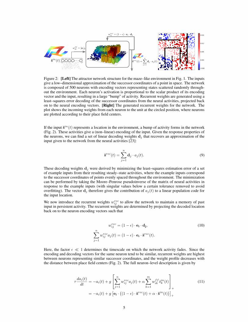
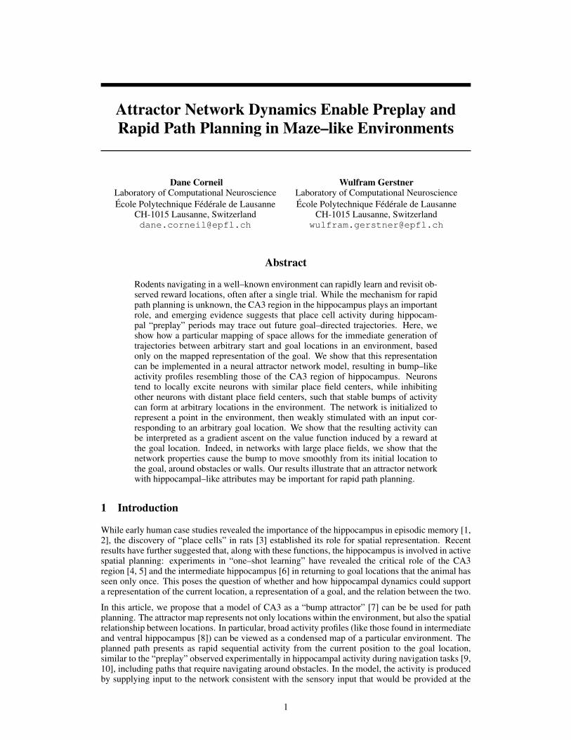
Figure 2: [Left] The attractor network structure for the maze–like environment in Fig. 1. The inputsgive a low–dimensional approximation of the successor coordinates of a point in space. The networkis composed of 500 neurons with encoding vectors representing states scattered randomly through-out the environment. Each neuron’s activation is proportional to the scalar product of its encodingvector and the input, resulting in a large “bump” of activity. Recurrent weights are generated using aleast–squares error decoding of the successor coordinates from the neural activities, projected backon to the neural encoding vectors. [Right] The generated recurrent weights for the network. Theplot shows the incoming weights from each neuron to the unit at the circled position, where neuronsare plotted according to their place field centers.

If the input sin(t) represents a location in the environment, a bump of activity forms in the network(Fig. 2). These activities give a (non–linear) encoding of the input. Given the response properties ofthe neurons, we can find a set of linear decoding weights dj that recovers an approximation of theinput given to the network from the neural activities [23]:

srec(t) =

n∑j=1

dj · aj(t). (9)

These decoding weights dj were derived by minimizing the least–squares estimation error of a setof example inputs from their resulting steady–state activities, where the example inputs correspondto the successor coordinates of points evenly spaced throughout the environment. The minimizationcan be performed by taking the Moore–Penrose pseudoinverse of the matrix of neural activities inresponse to the example inputs (with singular values below a certain tolerance removed to avoidoverfitting). The vector dj therefore gives the contribution of aj(t) to a linear population code forthe input location.

We now introduce the recurrent weights wrecij to allow the network to maintain a memory of past

input in persistent activity. The recurrent weights are determined by projecting the decoded locationback on to the neuron encoding vectors such that

wrecij = (1− ε) · ei · dj, (10)

n∑j=1

wrecij aj(t) = (1− ε) · ei · srec(t).

Here, the factor ε � 1 determines the timescale on which the network activity fades. Since theencoding and decoding vectors for the same neuron tend to be similar, recurrent weights are highestbetween neurons representing similar successor coordinates, and the weight profile decreases withthe distance between place field centers (Fig. 2). The full neuron–level description is given by

τdai(t)

dt= −ai(t) + g

n∑j=1

wrecij aj(t) + α

m∑k=1

wffik s

ink (t)

+

(11)

= −ai(t) + g[ei ·((1− ε) · srec(t) + α · sin(t)

)]+

5

where the α parameter corresponds to the input strength. If we consider the estimate of srec(t)recovered from decoding the activities of the network, we arrive at the update equation

τdsrec(t)

dt≈ α · sin(t)− ε · srec(t). (12)

Given a location sin(t) as an initial input, the recovered representation srec(t) approximates theinput and reinforces it, allowing a persistent bump of activity to form. When sin(t) then changesto a new (goal) location, the input and recovered coordinates conflict. By Eq. 12, the recoveredlocation moves in the direction of the new input, giving us an approximation of the initial gradientascent step in Eq. 6 with the addition of a decay controlled by ε. As we will show, the attractordynamics typically cause the network activity to manifest as a movement of the bump towards thegoal location, through locations intermediate to the starting position and the goal (as observed inexperiments [9, 10]). After a short stimulation period, the network activity can be decoded to give astate nearby the starting position that is closer to the goal. Note that, with no decay ε, the networkactivity will tend to grow over time. To induce stable activity when the network representationmatches the goal position (srec(t) ≈ sin(t)), we balanced the decay and input strength (ε = α).

In the following, we consider networks where the successor coordinate representation was truncatedto the first q dimensions, where q � n. This was done because the network is composed of a limitednumber of neurons, representing only the portion of the successor coordinate space correspondingto actual locations in the environment. In a very high–dimensional space, the network can rapidlymove into a regime far from any actual locations, and the integration accuracy suffers. In effect, theweight profiles and feed–forward activation profile become very narrow, and as a result the bumpof activity simply disappears from the original position and reappears at the goal. Conversely, low–dimensional representations tend to result in broad excitatory weight profiles and activity profiles(Fig. 2). The high degree of excitatory overlap across the network causes the activity profile to movesmoothly between distant points, as we will show.

4 Results

We generated attractor networks according to the layout of multiple environments containing wallsand obstacles, and stimulated them successively with arbitrary startpoints and goals. We usedn = 500 neurons to represent each environment, with place field centers selected randomly through-out the environment. The successor coordinates were generated using γ = 1. We adjusted q tocontrol the dimensionality of the representation. The network activity resembles a bump across aportion of the environment (Fig. 3). Low–dimensional representations (low q) produced large activ-ity bumps across significant portions of the environment; when a weak stimulus was provided at thegoal, the overall activity decreased while the center of the bump moved towards the goal throughthe intervening areas of the environment. With a high–dimensional representation, activity bumpsbecame more localized, and shifted discontinuously to the goal (Fig. 3, bottom row).

For several networks representing different environments, we initialized the activity at points evenlyspaced throughout the environment and provided weak feed–forward stimulation corresponding toa fixed goal location (Fig. 4). After a short delay (5τ ), we decoded the successor coordinates fromthe network activity to determine the closest state (Eq. 6). The shifts in the network representationare shown by the arrows in Fig. 4. For two networks, we show the effect of different feed–forwardstimuli representing different goal locations. The movement of the activity profile was similar to theshortest path towards the goal (Fig. 4, bottom left), including reversals at equidistant points (centerbottom of the maze). Irregularities were still present, however, particularly near the edges of theenvironment and in the immediate vicinity of the goal (where high–frequency components play alarger role in determining the value gradient).

5 Discussion

We have presented a spatial bump attractor model generalized to represent environments with arbi-trary obstacles, and shown how, with large activity profiles relative to the size of the environment, thenetwork dynamics can be used for path–finding. This provides a possible correlate for goal–directed

6

0.0

4.0

9.0

13.0

18.0

0.0

4.0

9.0

13.0

18.0

0.0

2.0

4.0

6.0

8.0

0.0

2.75

5.5

8.25

11.0

Figure 3: Attractor network activities illustrated over time for different inputs and networks, inmultiples of the membrane time constant τ . Purple boxes indicate the most active unit at each pointin time. [First row] Activities are shown for a network representing a maze–like environment ina low–dimensional space (q = 5). The network was initially stimulated with a bump of activa-tion representing the successor coordinates of the state at the black circle; recurrent connectionsmaintain a similar yet fading profile over time. [Second row] For the same network and initial con-ditions, a weak constant stimulus was provided representing the successor coordinates at the greycircle; the activities transiently decrease and the center of the profile shifts over time through theenvironment. [Third row] Two positions (black and grey circles) were sequentially activated in anetwork representing a second environment in a low–dimensional space (q = 4). [Bottom row] Fora higher–dimensional representation (q = 50), the activity profile fades rapidly and reappears at thestimulated position.

activity observed in the hippocampus [9, 10] and an hypothesis for the role that the hippocampusand the CA3 region play in rapid goal–directed navigation [4–6], as a complement to an additional(e.g. model–free) system enabling incremental goal learning in unfamiliar environments [4].

Recent theoretical work has linked the bump–like firing behaviour of place cells to an encoding of theenvironment based on its natural topology, including obstacles [22], and specifically to the successorrepresentation [14]. As well, recent work has proposed that place cell behaviour can be learned byprocessing visual data using hierarchical slow feature analysis [15, 16], a process which can extractthe lowest frequency eigenvectors of the graph Laplacian generated by the environment [20] andtherefore provide a potential input for successor representation–based activity. We provide the firstlink between these theoretical analyses and attractor–based models of CA3.

Slow feature analysis has been proposed as a natural outcome of a plasticity rule based on Spike–Timing–Dependent Plasticity (STDP) [24], albeit on the timescale of a standard postsynaptic po-

7

Figure 4: Large–scale, low–dimensional attractor network activities can be decoded to determinelocal trajectories to long–distance goals. Arrows show the initial change in the location of theactivity profile by determining the state closest to the decoded network activity (at t = 5τ ) afterweakly stimulating with the successor coordinates at the black dot (α = ε = 0.05). Pixels show theplace field centers of the 500 neurons representing each environment, coloured according to theiractivity at the stimulated goal site. [Top left] Change in position of the activity profile in a maze–like environment with low–dimensional activity (q = 5) compared to [Bottom left] the true shortestpath towards the goal at each point in the environment. [Additional plots] Various environmentsand stimulated goal sites using low–dimensional successor coordinate representations.

tential rather than the behavioural timescale we consider here. However, STDP can be extended tobehavioural timescales when combined with sustained firing and slowly decaying potentials [25] ofthe type observed on the single–neuron level in the input pathway to CA3 [26], or as a result ofnetwork effects. Within the attractor network, learning could potentially be addressed by a rule thattrains recurrent synapses to reproduce feed–forward inputs during exploration (e.g. [27]).

Our model assigns a key role to neurons with large place fields in generating long–distance goal–directed trajectories. This suggests that such trajectories in dorsal hippocampus (where place fieldsare much smaller [8]) must be inherited from dynamics in ventral or intermediate hippocampus.The model predicts that ablating the intermediate/ventral hippocampus [6] will result in a significantreduction in goal–directed preplay activity in the remaining dorsal region. In an intact hippocampus,the model predicts that long–distance goal–directed preplay in the dorsal hippocampus is precededby preplay tracing a similar path in intermediate hippocampus. However, these large–scale networkslack the specificity to consistently generate useful trajectories in the immediate vicinity of the goal.Therefore, higher–dimensional (dorsal) representations may prove useful in generating trajectoriesclose to the goal location, or alternative methods of navigation may become more important.

If an assembly of neurons projecting to the attractor network is active while the animal searches theenvironment, reward–modulated Hebbian plasticity provides a potential mechanism for reactivatinga goal location. In particular, the presence of a reward–induced neuromodulator could allow forpotentiation between the assembly and the attractor network neurons active when the animal receivesa reward at a particular location. Activating the assembly would then provide stimulation to the goallocation in the network; the same mechanism could allow an arbitrary number of assemblies tobecome selective for different goal locations in the same environment. Unlike traditional model–free methods of learning which generate a static value map, this would give a highly configurablemeans of navigating the environment (e.g. visiting different goal locations based on thirst vs. hungerneeds), providing a link between spatial navigation and higher cognitive functioning.

AcknowledgementsThis research was supported by the Swiss National Science Foundation (grant agreement no. 200020 147200).We thank Laureline Logiaco and Johanni Brea for valuable discussions.

8

References[1] William Beecher Scoville and Brenda Milner. Loss of recent memory after bilateral hippocampal lesions. Journal of

neurology, neurosurgery, and psychiatry, 20(1):11, 1957.

[2] Howard Eichenbaum. Memory, amnesia, and the hippocampal system. MIT press, 1993.

[3] John O’Keefe and Jonathan Dostrovsky. The hippocampus as a spatial map. preliminary evidence from unit activity inthe freely-moving rat. Brain research, 34(1):171–175, 1971.

[4] Kazu Nakazawa, Linus D Sun, Michael C Quirk, Laure Rondi-Reig, Matthew A Wilson, and Susumu Tonegawa.Hippocampal CA3 NMDA receptors are crucial for memory acquisition of one-time experience. Neuron, 38(2):305–315, 2003.

[5] Toshiaki Nakashiba, Jennie Z Young, Thomas J McHugh, Derek L Buhl, and Susumu Tonegawa. Transgenic inhibitionof synaptic transmission reveals role of ca3 output in hippocampal learning. Science, 319(5867):1260–1264, 2008.

[6] Tobias Bast, Iain A Wilson, Menno P Witter, and Richard GM Morris. From rapid place learning to behavioral perfor-mance: a key role for the intermediate hippocampus. PLoS biology, 7(4):e1000089, 2009.

[7] Alexei Samsonovich and Bruce L McNaughton. Path integration and cognitive mapping in a continuous attractor neuralnetwork model. The Journal of Neuroscience, 17(15):5900–5920, 1997.

[8] Kirsten Brun Kjelstrup, Trygve Solstad, Vegard Heimly Brun, Torkel Hafting, Stefan Leutgeb, Menno P Witter, Edvard IMoser, and May-Britt Moser. Finite scale of spatial representation in the hippocampus. Science, 321(5885):140–143,2008.

[9] Brad E Pfeiffer and David J Foster. Hippocampal place-cell sequences depict future paths to remembered goals. Nature,497(7447):74–79, 2013.

[10] Andrew M Wikenheiser and A David Redish. Hippocampal theta sequences reflect current goals. Nature neuroscience,2015.

[11] Louis-Emmanuel Martinet, Denis Sheynikhovich, Karim Benchenane, and Angelo Arleo. Spatial learning and actionplanning in a prefrontal cortical network model. PLoS computational biology, 7(5):e1002045, 2011.

[12] Filip Ponulak and John J Hopfield. Rapid, parallel path planning by propagating wavefronts of spiking neural activity.Frontiers in computational neuroscience, 7, 2013.

[13] Peter Dayan. Improving generalization for temporal difference learning: The successor representation. Neural Com-putation, 5(4):613–624, 1993.

[14] Kimberly L Stachenfeld, Matthew Botvinick, and Samuel J Gershman. Design principles of the hippocampal cognitivemap. In Z. Ghahramani, M. Welling, C. Cortes, N.D. Lawrence, and K.Q. Weinberger, editors, Advances in NeuralInformation Processing Systems 27, pages 2528–2536. Curran Associates, Inc., 2014.

[15] Mathias Franzius, Henning Sprekeler, and Laurenz Wiskott. Slowness and sparseness lead to place, head-direction, andspatial-view cells. PLoS Computational Biology, 3(8):e166, 2007.

[16] Fabian Schoenfeld and Laurenz Wiskott. Modeling place field activity with hierarchical slow feature analysis. Frontiersin Computational Neuroscience, 9:51, 2015.

[17] Richard S Sutton and Andrew G Barto. Introduction to reinforcement learning. MIT Press, 1998.

[18] Ronald R Coifman and Stephane Lafon. Diffusion maps. Applied and computational harmonic analysis, 21(1):5–30,2006.

[19] Sridhar Mahadevan. Learning Representation and Control in Markov Decision Processes, volume 3. Now PublishersInc, 2009.

[20] Henning Sprekeler. On the relation of slow feature analysis and laplacian eigenmaps. Neural computation, 23(12):3287–3302, 2011.

[21] John Conklin and Chris Eliasmith. A controlled attractor network model of path integration in the rat. Journal ofcomputational neuroscience, 18(2):183–203, 2005.

[22] Nicholas J Gustafson and Nathaniel D Daw. Grid cells, place cells, and geodesic generalization for spatial reinforcementlearning. PLoS computational biology, 7(10):e1002235, 2011.

[23] Chris Eliasmith and C Charles H Anderson. Neural engineering: Computation, representation, and dynamics in neu-robiological systems. MIT Press, 2004.

[24] Henning Sprekeler, Christian Michaelis, and Laurenz Wiskott. Slowness: an objective for spike-timing-dependentplasticity. PLoS Comput Biol, 3(6):e112, 2007.

[25] Patrick J Drew and LF Abbott. Extending the effects of spike-timing-dependent plasticity to behavioral timescales.Proceedings of the National Academy of Sciences, 103(23):8876–8881, 2006.

[26] Phillip Larimer and Ben W Strowbridge. Representing information in cell assemblies: persistent activity mediated bysemilunar granule cells. Nature neuroscience, 13(2):213–222, 2010.

[27] Robert Urbanczik and Walter Senn. Learning by the dendritic prediction of somatic spiking. Neuron, 81(3):521–528,2014.

9