attribute learning inlarge-scale datasets - stanford...

Attribute learning in large-scale datasets

Olga Russakovsky and Li Fei-Fei

Stanford University{olga,feifeili}@cs.stanford.edu

Abstract. We consider the task of learning visual connections betweenobject categories using the ImageNet dataset, which is a large-scaledataset ontology containing more than 15 thousand object classes. Wewant to discover visual relationships between the classes that are cur-rently missing (such as similar colors or shapes or textures). In this workwe learn 20 visual attributes and use them in a zero-shot transfer learningexperiment as well as to make visual connections between semanticallyunrelated object categories.

1 Introduction

Computer vision has traditionally focused on object categories: object classifica-tion, object segmentation, object retrieval, and so on. Recently, there has beensome interest in transitioning from learning visual nouns (whether object cate-gories, such as cars or pedestrians, or object parts, such as “wheel” or “head”)to visual adjectives (such as “red” or “striped” or “long”) which can be usedto describe a wide range of object categories [1–6]. Learning visual attributeshas been shown to be beneficial for improving performance of detectors [3] butespecially for transferring learned information between object categories. For ex-ample, learning the color “red” or the pattern “striped” from a series of trainingimages can then be used to recognize these attributes in a variety of unseenimages and object categories [1, 3].

The term “attribute” is defined in Webster’s dictionary as “an inherent char-acteristic” of an object, and various types of attributes have been explored inthe literature: appearance adjectives (such as color, texture, shape) [1–5, 7], pres-ence or absence of parts [1, 4, 6] and similarity to known object categories [1, 5,6]. Attributes have also been broken up into (1) semantic, i.e., those that can bedescribed using language [1, 4, 7], and (2) non-semantic but discriminative [3] orsimilarity-based [5, 6]. In this paper, we focus on semantic appearance attributes.

Attributes and parts-based models are particularly important when buildinglarge-scale systems, where it is infeasible to train an object classifier indepen-dently for each object class. Given a sufficiently rich dataset of learned adjectives,new categories of objects can be recognized simply from a verbal description con-sisting of a list of the attributes [1, 3] or a verbal description in combination withjust a few training examples [3].

In this paper, we consider learning multiple visual attributes on ImageNet [9],which is a large-scale ontology of images built uponWordNet [8]. It contains more

2 Attribute learning in large-scale datasets

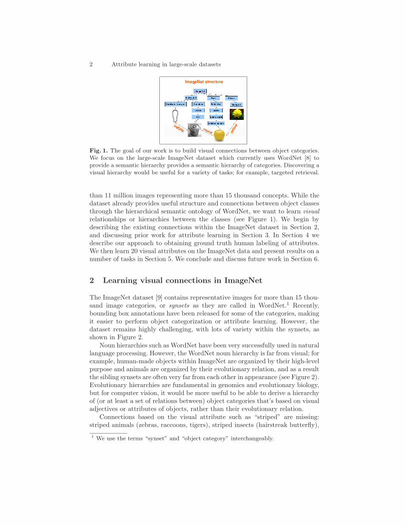
Fig. 1. The goal of our work is to build visual connections between object categories.We focus on the large-scale ImageNet dataset which currently uses WordNet [8] toprovide a semantic hierarchy provides a semantic hierarchy of categories. Discovering avisual hierarchy would be useful for a variety of tasks; for example, targeted retrieval.

than 11 million images representing more than 15 thousand concepts. While thedataset already provides useful structure and connections between object classesthrough the hierarchical semantic ontology of WordNet, we want to learn visual

relationships or hierarchies between the classes (see Figure 1). We begin bydescribing the existing connections within the ImageNet dataset in Section 2,and discussing prior work for attribute learning in Section 3. In Section 4 wedescribe our approach to obtaining ground truth human labeling of attributes.We then learn 20 visual attributes on the ImageNet data and present results on anumber of tasks in Section 5. We conclude and discuss future work in Section 6.

2 Learning visual connections in ImageNet

The ImageNet dataset [9] contains representative images for more than 15 thou-sand image categories, or synsets as they are called in WordNet.1 Recently,bounding box annotations have been released for some of the categories, makingit easier to perform object categorization or attribute learning. However, thedataset remains highly challenging, with lots of variety within the synsets, asshown in Figure 2.

Noun hierarchies such as WordNet have been very successfully used in naturallanguage processing. However, the WordNet noun hierarchy is far from visual; forexample, human-made objects within ImageNet are organized by their high-levelpurpose and animals are organized by their evolutionary relation, and as a resultthe sibling synsets are often very far from each other in appearance (see Figure 2).Evolutionary hierarchies are fundamental in genomics and evolutionary biology,but for computer vision, it would be more useful to be able to derive a hierarchyof (or at least a set of relations between) object categories that’s based on visualadjectives or attributes of objects, rather than their evolutionary relation.

Connections based on the visual attribute such as “striped” are missing:striped animals (zebras, raccoons, tigers), striped insects (hairstreak butterfly),

1 We use the terms “synset” and “object category” interchangeably.

Attribute learning in large-scale datasets 3

Edible fruit subtree

Fig synset Pineapple synset Mango synset Kiwi synset

Fig. 2. Example images of synsets that are direct descendants of the edible fruit synset.First, the high variability within each of the four synsets makes classification on thisdataset very challenging. Second, the four object classes are sibling synsets in WordNetsince they are all children of the “edible fruit” synset; however, visually they are quitedifferent from each other in terms of color, texture and shape.

striped flowers (butterfly orchid, moosewood tree), striped vegetables (cushaw,watermelon), striped fish (black sea bass, lionfish) and inanimate objects suchas striped fabric are not related within ImageNet. To the best of our knowl-edge, previous work on attributes has focused on making connections withina much more narrow set of object categories (such as animals [1, 6], cars [3, 4]or faces [5]). We are interested in discovering visual relations between all cate-gories of ImageNet, from fruits to animals to appliances to fabrics. We show inSection 5.4 that our algorithm indeed manages to do that.

3 Related work

Ferrari and Zisserman [2] proposed learning attributes using segments as the ba-sic building blocks. They distinguish between unary attributes (colors) involvingjust a single segment and binary attributes (stripes, dots and checkerboards)involving a pattern of alternating segments. Since their method relies on obtain-ing a near-perfect segmentation of the pattern, in practice it’s difficult to applyto challenging natural images – for example, the stripes of a tiger are very dif-ficult to segment out perfectly, and the orange background stripes would oftenget merged into a single segment, contrary to what their attribute classificationalgorithm expects.

Yanai and Barnard [7] learned the “visualness” of 150 concepts by performingprobabilistic region selection for images labeled as positive and negative examplesof a concept, and computing the entropy measure which represents how visualthis concept is. They evaluated their algorithm on Google search images, and alsoconsidered each image to be a collection of regions obtained from segmentation,but didn’t consider the pairwise relationship between the regions.

Recently, Lampert et al. [1] considered the problem of object classificationwhen the test set consists entirely of previously unseen object categories, and thetransfer of information from the training to the test phase occurs entirely throughattribute text labels. They introduced the Animal with Attributes dataset with30,000 images annotated with 50 classes. They are interested in performing zero-


shot object classification (where the object classes in the training and test setsare disjoint) based on attribute transfer rather than learning the attributes them-selves or building an attribute hierarchy. Interestingly, some of their attributesare not even fundamentally “visual” (for example, “strong” or “nocturnal”), butwere nevertheless found to be useful for classification [1]. One interesting thing topoint out in relation to our work is that ImageNet already has subtrees for someof their adjectives, such as edible, living, predator/prey/scavenger, young, do-mestic, male/female, even insectivore/omnivore/herbivore. While many of theirother attributes are animal-specific, such as “has paws,” and thus not as usefulin our setting for making connections between a broad range of object categories,we were inspired by their list in creating our own.

Farhadi et al. [3] worked on describing objects by parts, such as “has head,”or appearance adjectives, such as “spotty.” They wanted to both describe unfa-miliar objects (such as “hairy and four-legged”) and learn new categories withfew visual examples. They distinguished between two types of attributes: seman-tic (“spotty”) and discriminative (dogs have it but cat don’t). Similarly, Kumaret al. [5] considered two types of attributes for face recognition: those trained torecognize specific aspects of visual appearance, such as gender or race, and “sim-ile” classifiers which represent the similarity of faces to celebrity faces. We focuson semantic attributes in the current work, but argue that ultimately discrimi-native and comparative attributes are necessary because language is insufficientto precisely describe, e.g., the typical shape of a car or the texture of a fish.

Rohrbach et al. [6] use semantic relationships mined from language to achieveunsupervised knowledge transfer. They found that path length in WordNet is apoor indicator of attribute association (for example, the “tusk” synset is veryfar from the “elephant” synset in the hierarchy, making it impossible to inferthat elephants would have tusks). They show that web search for part-whole re-lationships is a better way of mining attribute annotations for object categories.In our work, we also explore using WordNet to mine attribute associations, butconsider using the WordNet synset definitions rather than path length.

Most recently, Farhadi et al. [4] discussed creating the right level of abstrac-tion for knowledge transfer. They learned part and category detectors of objects,and described objects by spacial arrangement of their attributes and the inter-action between them. They focused on finding animal and vehicle categories notseen during training, and inferring attributes such as function and pose. Theylearn both the parts that are visible and not visible in each image.

4 Building and labeling an attribute dataset

In order to learn and evaluate attribute labels, we first need to obtain groundtruth annotations of the images. [6] discusses various data mining strategies;however, it focuses on parts-based attributes, mining for relations such as “legis a part of dog” or “dog’s leg.” WordNet provides a definition for every synsetit contains; since we are instead interested in appearance-based attributes, weconsidered two strategies: mining these definitions directly (which is different


than the path length discussed in [6]), and manual labeling (which was theapproach of [1, 4]).

WordNet synset definitions are not well-suited for mining visual adjectivesfor several reasons. First, the mined adjectives don’t necessarily correspond tovisual characteristics of the full object and require understanding of the objectparts (e.g., animals with a “striped tail”). Second, the mined adjectives oftenneed to be understood in the context of other adjectives in the definition (e.g.,a flower described as “yellow or red or blue”). Also, sometimes the adjectivesare extremely difficult to detect visually (e.g., a flag is defined as “rectangular”but usually doesn’t look rectangular in the image). However, since ImageNetis a very large-scale dataset, mining for attributes in this very simple way canhelp restrict attention to just a subset of the ImageNet data which is likely tocontain a sufficient amount of positive examples for each attribute. To constructthe dataset of 384 synsets that we use for our experiments, for every attributewe searched for all synsets (from among those with available bounding box an-notations) which contained this attribute in either the synset name or the synsetdefinition, and included that synset along with all of its siblings in the trainingset. The motivation for including the siblings was to provide a rich enough setof negative examples that are likely to differ from the positive synsets in onlya few characteristics, and specifically in the characteristic corresponding to themined attribute. For example, if a zebra is characterized as a “striped” equine,it’s reasonable to infer that other equines, such as horses, are not striped.

In order to obtain the ground truth data we use workers on Amazon Me-chanical Turk (AMT) to label 25 images randomly chosen from each synset. Wepresent each worker with 106 images (25 each from 4 different synsets plus 6randomly injected quality control images) and one attribute, and ask to make abinary decision of whether or not this attribute applies to the image. For colorattributes (black, blue, brown, gray, green, orange, pink, red, violet, white andyellow), we ask whether a significant part of the object (at least 25%) is thatcolor. For all other attributes (furry, long, metallic, rectangular, rough, round,shiny, smooth, spotted, square, striped, vegetation, wet, wooden), we ask if theywould describe the object as a whole using that attribute.

Each image is labeled by 3 workers, and we consider an image to be positive(negative) if all workers agree that it’s positive (negative); otherwise, we considerit ambiguous and don’t include it in our training sets. Unfortunately, for 5 of ourattributes (blue, violet, pink, square and vegetation) we did not get sufficientpositive training data (at least 75 images) to include them in our experiments.

We analyze the overlap between the mined synsets and the human labelingin Table 1. We consider a synset to be labeled positive for an attribute byAMT workers if more than half of its labeled images are unanimously labeledas positive. Interestingly, some obvious annotations such as “green salad” or“striped zebra” were not present in the human labels. This shows that dataobtained from AMT can be extremely noisy, and that better quality controland/or more annotators are needed. Currently we are only considering an imageto be a positive or negative example if it is labeled unambiguously; while this


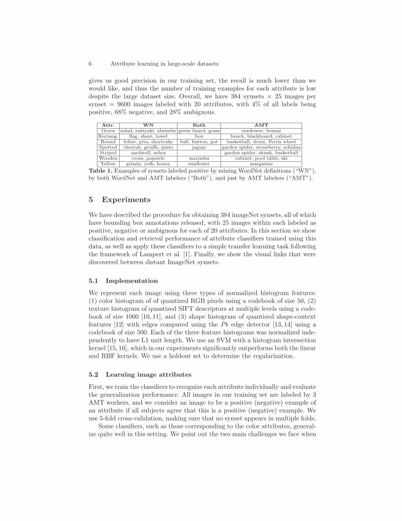
gives us good precision in our training set, the recall is much lower than wewould like, and thus the number of training examples for each attribute is lowdespite the large dataset size. Overall, we have 384 synsets × 25 images persynset = 9600 images labeled with 20 attributes, with 4% of all labels beingpositive, 68% negative, and 28% ambiguous.

Attr. WN Both AMT

Green salad, sukiyaki, absinthe green lizard, grass sunflower, bonsai

Rectang. flag, sheet, towel box bench, blackboard, cabinet

Round feline, pita, shortcake ball, button, pot basketball, drum, Ferris wheel

Spotted cheetah, giraffe, pinto jaguar garden spider, strawberry, echidna

Striped aardwolf, zebra garden spider, skunk, basketball

Wooden cross, popsicle marimba cabinet, pool table, ski

Yellow grizzly, yolk, honey sunflower margarine

Table 1. Examples of synsets labeled positive by mining WordNet definitions (“WN”),by both WordNet and AMT labelers (“Both”), and just by AMT labelers (“AMT”).

5 Experiments

We have described the procedure for obtaining 384 imageNet synsets, all of whichhave bounding box annotations released, with 25 images within each labeled aspositive, negative or ambiguous for each of 20 attributes. In this section we showclassification and retrieval performance of attribute classifiers trained using thisdata, as well as apply these classifiers to a simple transfer learning task followingthe framework of Lampert et al. [1]. Finally, we show the visual links that werediscovered between distant ImageNet synsets.

5.1 Implementation

We represent each image using three types of normalized histogram features:(1) color histogram of of quantized RGB pixels using a codebook of size 50, (2)texture histogram of quantized SIFT descriptors at multiple levels using a code-book of size 1000 [10, 11], and (3) shape histogram of quantized shape-contextfeatures [12] with edges computed using the Pb edge detector [13, 14] using acodebook of size 500. Each of the three feature histograms was normalized inde-pendently to have L1 unit length. We use an SVM with a histogram intersectionkernel [15, 16], which in our experiments significantly outperforms both the linearand RBF kernels. We use a holdout set to determine the regularization.

5.2 Learning image attributes

First, we train the classifiers to recognize each attribute individually and evaluatethe generalization performance. All images in our training set are labeled by 3AMT workers, and we consider an image to be a positive (negative) example ofan attribute if all subjects agree that this is a positive (negative) example. Weuse 5-fold cross-validation, making sure that no synset appears in multiple folds.

Some classifiers, such as those corresponding to the color attributes, general-ize quite well in this setting. We point out the two main challenges we face when


(a) (b)

Fig. 3. (a) Performance of attribute classifiers (as measured by the area under the ROCcurve) sorted by attribute type. The average performance of each type is reported inparentheses. (b) Some example images labeled by the human subjects as “striped.”This shows the difficultly of learning a good “striped” classifier on this dataset.

training the attribute classifiers. First, the “pattern” classifiers corresponding to“striped” and “spotted” attributes perform poorly as a result of the great vari-ety of the exemplars (see Figure 3(b) for examples of “striped” images). Thereis a lack of training data especially in light of this variety (only 99 images werelabeled as “striped” and 146 as “spotted”). As the number of object categoriesincreases, so does the variety of appearances of certain attributes, and thus theamount of training data collected should be sufficient to account for this.

Second, the two texture attributes “rough” and “smooth” suffer from ambi-

guity as evidenced by the lack of labeling consensus. The labelers unanimouslyagreed on only 66% of the images in the dataset when labeling with the “smooth”attribute, and 72% when labeling with the “rough” attribute. In contrast, forevery other attribute the annotators unanimously agreed on more than 79% ofthe images. As a result, whether an image was labeled as a positive or negativetraining example for “rough” or “smooth” was largely dependent on the specificset of labelers assigned to it. Such attributes require further refinement and/orbetter definitions during the labeling process.

In Figures 4-6 we show qualitative retrieval results using the trained clas-sifiers. Note that many of the top correctly retrieved images were not used inthe quantitative evaluation because they were not unanimously labeled by thelabelers. This further reinforces the need for more rigorous labeling procedures.

5.3 Transfer learning using attributes

We use the learned classifiers in a small-scale transfer learning experiment fol-lowing the Direct attribute prediction (DAP) model of Lampert et al. [1]. Briefly,we are given L test classes z1,...,L not seen during training, and M attributes,where the test classes are annotated with binary labels alm for each class l andattribute m. In our experiments we consider L = 5 test classes: chestnut, greenlizard, honey badger, zebra, and spitz, and M = 20 attributes described above.


furry rectangular

metallic orange

Fig. 4. Visualization of four of the learned attributes (for the other attributes, seeFigures 5 and 6). For each attribute, the 5 rows represent the 5 training folds, andeach row shows the top 8 images retrieved from among all synsets that didn’t appearin that fold’s training set. The border around each image corresponds to the humanlabeler annotation (green is positive, red is negative, yellow is ambiguous).

The synset-level annotations come from AMT human labelers.2 We use 25 im-ages per object class as above, Given an image x, the DAP model defines theprobability of this image belonging to class z as

p(z|x) =∑

a∈{0,1}M

p(z|a)p(a|x) =p(z)

p(az)

M∏

m=1

p(azm|x)

where p(azm|x) is given by the learned attribute model, p(z) is assumed to be auniform class prior, and p(az) is the prior on seeing an example with the same setof attributes as the ground truth for the target class z, computed from trainingdata assuming a factorial distribution over attributes. Image x is assigned toclass c(x) using:

c(x) = argmaxl=1,...,L

M∏

m=1

p(azlm|x)

p(azlm)

2 Out of 100 class-attribute labels, 18 were ambiguous, meaning that less than half theimages within that class were unanimously annotated as either positive or negativefor that attribute by all 3 workers. We manually disambiguated the annotations.


black brown

gray green

long red

rough round

Fig. 5. Continuation of Figure 4 visualizing the learned attributes.


shiny smooth

spotted striped

wet white

wooden yellow

Fig. 6. Continuation of Figures 4 and 5 visualizing the learned attributes.


We apply this model to our learned classifiers and report our result in Ta-ble 2. The main source of errors is the zebra class, which relies on the poorlygeneralizing “striped” attribute (see results in Figure 3).

chestnut: brown,smooth 0.52 0.16 0.12 0.12 0.08

green lizard: green, long 0 0.84 0 0.12 0.04

honey badger: black, gray, rough, furry 0.32 0 0.60 0.04 0.04

zebra: black, white, striped, smooth 0.36 0.08 0.40 0.08 0.08

spitz: white, furry 0.08 0 0.36 0.08 0.48

Table 2. On the left are the animal classes and the corresponding human attributeannotations, and on the right is the confusion table from the transfer learning exper-iments. The rows of the confusion table are the ground truth labels and the columnsare the classifier outputs.

5.4 Synset-level connections

Given the attribute classifiers we can now consider making synset-level connec-tions within ImageNet, which was the main objective of our work. For eachattribute, we have 5 learned classifiers, one for each of the 5 folds. We fit a sig-moid to the output of each classifier to obtain normalized probabilities [15, 17].We run each classifier on all images that were not part of its training set synsets.For each test synset, we compute the median confidence score of the classifieron images within that synset. Figures 7 and 8 show the top returned synsets.

There are various interesting observations that could be made about the re-trieved synsets. “Green,” “white” and “round” classifiers discover connectionsbetween synsets which are very far apart in the WordNet hierarchy – for exam-ple, salad, which is a node 6 levels deep under the “food, nutrient” subtree ofImageNet, green lizard, which is 13 levels deep under the “animal” subtree, andbonsai, which is 9 levels deep under the “tree” subtree. Similarly, the “white”classifier connects various breeds of dogs as well as Persian cats, sails, and sheets.The round classifier connects, e.g., basketball, ramekin, which is “a cheese dishmade with egg and bread crumbs that is baked and served in individual fireproofdishes” [8], and egg yolk.

More interesting is to look at attributes such as “long,” which are morecontextual and relative, and see the kinds of synsets that were learned. It is notimmediately clear that the classifier is picking up on the synsets that humanwould classify as “long,” although bottles and forks definitely are.

Finally, “striped” and “wet” discovered some interesting connections – eventhough it is extremely difficult to learn the high variability of stripes in natural


green

salad (.84), green lizard (.73), bonsai (.52), pesto (.43), saute (.37), daisy (.30)pot-au-feu (.12), salsa (.12), roughage (.11), cow (.11)

white

kuvasz (.70), Saint Bernard (.67), clumber (.65), wirehair (.62), foxhound (.60)sheet (.49), gerbil (.48), Persian cat (.48), sail (.45), bullterrier (.43)

round

egg yolk (.75), basketball (.68), button (.63), goulash (.56), basket (.49),ramekin (.47), ball (.42), pot (.42), veloute (.39), miso (.37)

long

kirsch (.83), sail (.77), rorqual (.74), police van (.72), fork (.69), rack (.67),killer whale (.58), window (.54), transporter (.50), pool table (.49)

striped

barn spider (.36), daisy (.17), zebra (.17), echidna (.16), backboard (.13),drum (.12), coloring (.12), roller coaster (.12), bridge (.11), colobus (.11)

wet

rorqual (.59), sidecar (.55), orangeade (.53), flan (.52), screwdriver (.47), killerwhale (.44), bowhead (.43), maraschino (.41), dugong (.40), porpoise (.40)

Fig. 7. This figure shows the top 10 synsets that were returned by the algorithm asthe most representative for a subset of the attributes (see Figure 8 for the remainder).The number in parenthesis represents the median probability assigned to images withinthat synset by the attribute classifier.

scenes, zebras and echidnas were retrieved, as well as “garden spiders,” whichactually often do look striped upon inspection even though it is not a commonexample that humans would think of as a striped insect. The “wet” classifierespecially was able to pick up on some very promising connections: besides justlearning that the ocean tends to be wet and thus marine animals are likely wet,it also made the connection to cocktail drinks such as sidecar and screwdriver.

6 Conclusion

In this work we began building a set of visual connections between object cat-egories on a large scale dataset. Our ultimate goal is to automatically discovera large variety of visual connections between thousands of object categories.


black

colobus (.78), siamang (.75), guereza (.73), groenendael (.71), binturong (.69), chimpanzee (.66),schipperke (.66), silverback (.63), aye-aye (.54), gorilla (.54), skunk (.53), bowhead (.50)

brown

puku (.82), lechwe (.73), kob (.73), steenbok (.66), sassaby (.65), redbone (.62),bushbuck (.60), ragout (.59), dhole (.57), chestnut (.56), bovid (.54), sambar (.54)

furry

keeshond (.94), chacma (.93), macaque (.90), grivet (.90), grizzly (.88), gorilla (.88),baboon (.88), mandrill (.88), koala (.86), simian (.86), guenon (.85), kit fox (.85)

gray

koala (.42), abrocome (.39), gorilla (.38), grivet (.33), keeshond (.29), manul (.29),schnauzer (.29), chacma (.29), viscacha (.28), vervet (.28), hominid (.27), otter (.26)

metallic

fork (.72), transporter (.56), roller coaster (.49), stick (.41), wheel (.38), police van (.37),keyboard (.34), sail (.31), bridge (.31), building (.28), ski (.25), bowhead (.25)

orange

orangeade (.73), egg yolk (.58), sunflower (.44), strawberry (.43), fork (.42), maraschino (.42),casserole (.39), screwdriver (.37), pizza (.35), croquette (.30), vermouth (.30), moussaka (.29)

rectangular

police van (.90), transporter (.84), cabinet (.61), marimba (.50), window (.44), varietal (.42),flag (.38), bridge (.38), kummel (.31), pot (.29), generic (.28), pool table (.26)

red

shortcake (.70), basketball (.67), catsup (.55), teriyaki (.43), salad (.42), pizza (.37),chili (.30), flan (.26), ragout (.23), slumgullion (.22), bordelaise (.20), police van (.18)

rough

fork (.11), ski (.11), transporter (.11), sail (.11), rorqual (.11), bowhead (.11),keyboard (.11), cross (.11), killer whale (.11), roller coaster (.11), narwhal (.11), stick (.11)

shiny

rorqual (.95), bowhead (.82), killer whale (.61), dugong (.54), narwhal (.52), manatee (.44),porpoise (.31), police van (.27), kirsch (.27), flag (.21), stick (.21), ski (.20)

smooth

sail (.65), kirsch (.64), varietal (.63), champagne (.62), generic (.61), green lizard (.58),bottle (.56), egg yolk (.55), window (.55), mallet (.54), pool table (.53), tower (.53)

spotted

barn spider (.37), zebra (.26), Ferris wheel (.24), cheetah (.19), insectivore (.16), badger (.15),carnivore (.15), grass (.15), kudu (.14), groundhog (.13), pesto (.12), dik-dik (.12)

wooden

fork (.75), rack (.66), bridge (.54), police van (.52), pool table (.46), table (.43),kirsch (.42), marimba (.40), squash racket (.36), transporter (.35), cue (.35), slivovitz (.27)

yellow

egg yolk (1.00), sunflower (.86), omelet (.70), kedgeree (.64), flan (.61), tostada (.48),succotash (.42), pizza (.35), zabaglione (.26), ravigote (.25), curry (.23), casserole (.21)

Fig. 8. Continuation of Figure 7 showing the visual connections made between synsets.


Discovering semantic attributes can aid in more intelligent image retrieval: forexample, the user can specify exactly what he’s looking for using a known dic-tionary of attributes instead of visual training examples. More interestingly,clustering the attributes into categories, such as shape, texture, color, and soon, and working with non-semantic attributes, can potentially lead to at leasttwo major advantages. First, this can allow for new ways of object classificationtraining: instead of showing the algorithm a large variety of cars during training,one can simply inject a bit of prior knowledge that cars can come in all colors butshape is the important characteristic. Second, in retrieval, instead of asking tofind an image closest to the query, the user can instead specify that he’s lookingfor something that’s close in color to the query image, but round.

Acknowledgements We give warm thanks to Alex Berg, Jia Deng, BangpengYao and Li-Jia Li for their help with this work. Olga Russakovsky was supportedby the NSF graduate fellowship.

References

1. Lampert, C., Nickisch, H., Harmeling, S.: Learning to detect unseen object classesby between-class attribute transfer. CVPR (2009)

2. Ferrari, V., Zisserman, A.: Learning Visual Attributes. In: NIPS. (2007)3. Farhadi, A., Endres, I., Hoiem, D., Forsyth, D.: Describing objects by their at-

tributes. In: CVPR. (2009)4. Farhadi, A., Endres, I., Hoiem, D.: Attribute-Centric Recognition for Cross-

category Generalization. In: CVPR. (2010)5. Kumar, N., Berg, A.C., Belhumeur, P.N., Nayar, S.K.: Attribute and Simile Clas-

sifiers for Face Verification. In: ICCV. (2009)6. Rohrbach, M., Stark, M., Szarvas, G., Gurevych, I., Schiele, B.: What Helps Where

– And Why? Semantic Relatedness for Knowledge Transfer. CVPR (2010)7. Yanai, K., Barnard, K.: Image Region Entropy: A Measure of Visualness of Web

Images Associated with One Concept. In: ACM Multimedia. (2005)8. Fellbaum, C.: WordNet:An Electronic Lexical Database. Bradford Books (1998)9. Deng, J., Dong, W., Socher, R., Li, L.J., Li, K., Fei-Fe, L.: ImageNet: A Large-Scale

Hierarchical Image Database. CVPR (2009)10. Lowe, D.G.: Distinctive image features from scale-invariant keypoints. IJCV (2004)11. Berg, A., Deng, J., Fei-Fei, L.: ImageNet Large Scale Visual Recognition Challenge

development kit (2010)12. Belongie, S., Malik, J., Puzicha, J.: Shape matching and object recognition using

shape contexts. PAMI (2002)13. Martin, D., Fowlkes, C., , Malik, J.: Learning to detect natural image boundaries

using brightness and texture. NIPS (2002)14. Catanzaro, B., Su, B.Y., Sundaram, N., Lee, Y., Murphy, M., Keutzer, K.: Efficient,

high-quality image contour detection. ICCV (2009)15. Chang, C.C., Lin, C.J.: LIBSVM: a library for support vector machines (2001)16. Swain, M.J., Ballard, D.H.: Color indexing. IJCV (1991)17. Platt, J.: Probabilistic outputs for support vector machines and comparison to

regularized likelihood methods. Advances in Large Margin Classifiers (2000)

attribute learning inlarge-scale datasets - stanford...

Documents