attribute measurement error analysis -...

310 C hap te r N i n e

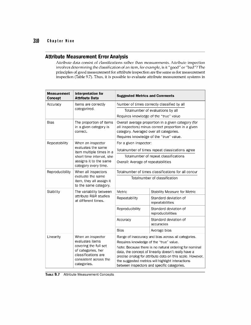
Attribute Measurement Error Analysis Attribute data consist of classifications rather than measurements. Attribute inspection involves determining the classification of an item, for example, is it "good" or "bad"? The principles of good measurement for attribute inspection are the same as for measurement inspection (Table 9.7). Thus, it is possible to evaluate attribute measurement systems in

Measurement Interpretation for Suggested Metrics and Comments

Concept Attribute Data

Accuracy Items are correctly Number of times correctly classified by all categorized. Totalnumber of evaluations by all

Requires knowledge of the "true" value

Bias The proportion of items Overall average proportion in a given category (for in a given category is all inspectors) minus correct proportion in a given correct. category. Averaged over all categories.

Requires knowledge of the "true" value.

Repeatability When an inspector For a given inspector: evaluates the same

Totalnumber of times repeat classications agree item multiple times in a short time interval, she Totalnumber of repeat classifications assigns it to the same Overall: Average of repeatabilities category every time.

Reproducibility When all inspectors Totalnumber of times classifications for all concur evaluate the same Totalnumber of classification item, they all assign it to the same category.

Stability The variability between Metric Stability Measure for Metric attribute R&R studies Repeatability Standard deviation of at different times. repeatabilities

Reproducibility Standard deviation of reproducibilities

Accuracy Standard deviation of accuracies

Bias Average bias

Linearity When an inspector Range of inaccuracy and bias across all categories. evaluates items Requires knowledge of the "true" value. covering the full set Note: Because there is no natural ordering for nominal of categories, her data, the concept of linearity doesn't really have a classifications are precise analog for attribute data on this scale. However, consistent across the the suggested metrics will highlight interactions categories. between inspectors and specific categories.

TABLE 9.7 Attribute Measurement Concepts

Measurement Systems Evaluation 311

much the same way as we evaluate variable measurement systems. Much less work has been done on evaluating attribute measurement systems. The proposals provided in this book are those I've found to be useful for my employers and clients. The ideas are not part of any standard and you are encouraged to think about them critically before adopting them. I also include an example of Minitab's attribute gage R&R analysis.

Operational Definitions An operational definition is defined as a requirement that includes a means of measurement. "High quality solder" is a requirement that must be operationalized by a clear definition of what "high quality solder" means. This might include verbal descriptions, magnification power, photographs, physical comparison specimens, and many more criteria.

Examples of Operational Definitions 1. Operational definition of the Ozone Transport Assessment Group's (OTAG) goal

Goal: To identify reductions and recommend transported ozone and its precursors which, in combination with other measures, will enable attainment and maintenance of the ozone standard in the OTAG region.

Suggested operational definition of the goal:

1. A general modeled reduction in ozone and ozone precursors aloft throughout the OTAG region; and

2. A reduction of ozone and ozone precursors both aloft and at ground level at the boundaries of non-attainment area modeling domains in the OTAG region; and

3. A minimization of increases in peak ground level ozone concentrations in the OTAG region (This component of the operational definition is in review.) .

2. Wellesley College Child Care Policy Research Partnership operational definition of unmet need

1. Standard of comparison to judge the adequacy of neighborhood services: the median availability of services in the larger region (Hampden County).

2. Thus, our definition of unmet need: The difference between the care available in the neighborhood and the median level of care in the surrounding region (stated in terms of child care slots indexed to the age-appropriate child population-" slots-per-tots").

3. Operational definitions of acids and bases

1. An acid is any substance that increases the concentration of the H+ ion when it dissolves in water.

2. A base is any substance that increases the concentration of the OH- ion when it dissolves in water.

4. Operational definition of "intelligence"

1. Administer the Stanford-Binet IQ test to a person and score the result. The person's intelligence is the score on the test.

5. Operational definition of "dark blue carpet"


A carpet will be deemed to be dark blue if

1. Judged by an inspector medically certified as having passed the U.s. Air Force test for color-blindness

1.1. It matches the PANTONE color card 7462 C when both carpet and card are illuminated by GE "cool white" fluorescent tubes;

1.2. Card and carpet are viewed at a distance between 16 and 24 inches.

How to Conduct Attribute Inspection Studies Some commonly used approaches to attribute inspection analysis are shown in Table 9.8.

Example of Attribute Inspection Error Analysis Two sheets with identical lithographed patterns are to be inspected under carefully controlled conditions by each of the three inspectors. Each sheet has been carefully examined multiple times by journeymen lithographers and they have determined that one of the sheets should be classified as acceptable, the other as unacceptable. The inspectors sit on a stool at a large table where the sheet will be mounted for inspection. The inspector can adjust the height of the stool and the angle of the table. A lighted magnifying glass is mounted to the table with an adjustable arm that lets the inspector move it to any part of the sheet (see Fig. 9.20).

Each inspector checks each sheet once in the morning and again in the afternoon. After each inspection, the inspector classifies the sheet as either acceptable or unacceptable. The entire study is repeated the following week. The results are shown in Table 9.9.

In Table 9.9 the part column identifies which sheet is being inspected, and the standard column is the classification for the sheet based on the journey-men's evaluations. A 1 indicates that the sheet is acceptable, a 0 that it is unacceptable. The columns labeled InspA, InspB, and InspC show the classifications assigned by the three inspectors respectively. The reproducible column is a 1 if all three inspectors agree on the classification, whether their classification agrees with the standard or not. The accurate column is a 1 if all three inspectors classify the sheet correctly as shown in the standard column.

Individual Inspector Accuracy Individual inspector accuracy is determined by comparing each inspector 's classification with the standard. For example, in cell C2 of Table 9.9 inspector A classified the unit as acceptable, and the standard column in the same row indicates that the classification is correct. However, in cell C3 the unit is classified as unacceptable when it actually is acceptable. Continuing this evaluation shows that inspector A made the correct assessment 7 out of 8 times, for an accuracy of 0.875 or 87.5%. The results for all inspectors are given in Table 9.10.

Repeatability and Pairwise Reproducibility Repeatability is defined in Table 9.7 as the same inspector getting the same result when evaluating the same item more than once within a short time interval. Looking at InspA


True Value Method of Evaluation Comments

Expert Judgment: An D Metrics: expert looks at the 1. Percent correct classifications after D Quantifies the accuracy of the classifications the operator makes

D Simple to evaluate normal classifications and decides which are D Who says the expert is correct?

correct and which are D Care must be taken to include all types of attributes

incorrect. D Difficult to compare operators since different units are classified by different people

D Acceptable level of performance must be decided upon. Consider cost, impact on customers, etc

Known Round Robin Study: D Metrics: A set of carefully 1. Percent correct by inspector identified objects is 2. Inspector repeatability chosen to represent

3. Inspector reproducibility the full range of attributes. 4. Stability

1. Each item is 5. Inspector "linearity"

evaluated by an expert D Full range of attributes included

and its condition D All aspects of measurement error quantified recorded. D People know they're being watched, may affect 2. Each item is performance evaluated by every D Not routine conditions inspector at least D Special care must be taken to insure rigor twice.

D Acceptable level of performance must be decided upon for each type of error. Consider cost, impact on customers, etc

D Metrics:

1. Inspector repeatability

2. Inspector reproducibility

3. Stability

4. Inspector "linearity"

Inspector D Like a round robin, except true value isn't known Concurrence Study: D No measures of accuracy or bias are possible. Can A set of carefully only measure agreement between equally qualified identified objects is people chosen to represent D Full range of attributes included the full range of

D People know they're being watched, may affect Unknown attributes, to the

performance extent possible.

1. Each item is D Not routine conditions

evaluated by every D Special care must be taken to insure rigor

inspector at least D Acceptable level of performance must be decided

twice. upon for each type of error. Consider cost, impact on customers, etc

TABLE 9.8 Methods of Evaluating Attribute Inspection


FIGURE 9.20 Lithography inspection station table, stool and magnifying glass.

A B C D E F G H I

1 Part Standard InspA InspB InspC Date Time Reproducible Accurate

2 1 1 1 1 1 Today Morning 1 1

3 1 1 0 1 1 Today Afternoon 0 0

4 2 0 0 0 0 Today Morning 1 1

5 2 0 0 0 1 Today Afternoon 0 0

6 1 1 1 1 1 Last Morning 1 1 Week

7 1 1 1 1 0 Last Afternoon 0 0 Week

8 2 0 0 0 1 Last Morning 0 0 Week

9 2 0 0 0 0 Last Afternoon 1 1 Week

TABLE 9.9 Results of Lithography Attribute Inspection Study

Inspector A B C

Accuracy 87.5% 100.0% 62.5%

TABLE 9.10 Inspector Accuracies

we see that when she evaluated Part 1 in the morning of "Today" she classified it as acceptable (I), but in the afternoon she said it was unacceptable (0). The other three morning/afternoon classifications matched each other. Thus, her repeatability is 3/4 or 75%.


Overall Today Last Week

A B C A B C A B C

A 0.75 0.88 0.50 A 0.50 0.75 0.50 A 1.00 1.00 0.50

B 1.00 0.50 B 1.00 0.75 B 1.00 0.50

C 0.25 C 0.50 C 0.00

TABLE 9.11 Repeatability and Pairwise Reproducibility for Both Days Combined

Pairwise reproducibility is the comparison of each inspector with every other inspector when checking the same part at the same time on the same day. For example, on Part l/Morning/Today, InspA's classification matched that of InspB. However, for Part 1/ Afternoon/Today InspA's classification was different than that of InspB. There are eight such comparisons for each pair of inspectors. Looking at InspA versus InspB we see that they agreed 7 of the 8 times, for a pairwise repeatability of 7/8 = 0.875.

In Table 9.11 the diagonal values are the repeatability scores and the off-diagonal elements are the pairwise reproducibility scores. The results are shown for "Today," "Last Week" and both combined.

Overall Repeatability, Reproducibility, Accuracy and Bias Information is always lost when summary statistics are used, but the data reduction often makes the tradeoff worthwhile. The calculations for the overall statistics are operationally defined as follows:

• Repeatability is the average of the repeatability scores for the 2 days combined; that is, (0.75 + 1.00 + 0.25)/3 = 0.67.

• Reproducibility is the average of the reproducibility scores for the 2 days combined (see Table 9.9); that is,

• Accuracy is the average of the accuracy scores for the 2 days combined (see Table 9.9); that is,

(1+0:0+0 + 1+0:0+0)/2=0.25

• Bias is the estimated proportion in a category minus the true proportion in the category. In this example the true percent defective is 50% (1 part in 2) . Of the 24 evaluations, 12 evaluations classified the item as defective. Thus, the bias is 0.5 - 0.5 = 0

Overall Stability Stability is calculated for each of the above metrics separately, as shown in Table 9.12.


Stabilityof ... Operational Definition of Stability Stability Result

Repeatability Standard deviation of the six repeatabilities (0.5, 1, 0.5, 1, 1, 1) 0.41

Reproducibility Standard deviation of the average repeatabilities. For data in 0.00 Table 9.9, STDEV [(VERAGE (H2:H5), AVERAGE (H6:H9)]

Accuracy Standard deviation of the average accuracies. For data in 0.00 Table 9.9, = STDEV [AVERAGE (2:5), AVERAGE (6:9)]

Bias Average of bias over the 2 weeks 0.0

TABLE 9.12 Stability Analysis

Interpretation of Results 1. The system overall appears to be unbiased and accurate. However, the evalua

tion of individual inspectors indicates that there is room for improvement.

2. The results of the individual accuracy analysis indicate that inspector C has a problem with accuracy, see Table 9.10.

3. The results of the R&R (pairwise) indicate that inspector C has a problem with both repeatability and reproducibility, see Table 9.11.

4. The repeatability numbers are not very stable (Table 9.12). Comparing the diagonal elements for Today with those of Last Week in Table 9.11, we see that inspectors A and C tended to get different results for the different weeks. Otherwise the system appears to be relatively stable.

5. Reproducibility of inspectors A and B is not perfect. Some benefit might be obtained from looking at reasons for the difference.

6. Since inspector B's results are more accurate and repeatable, studying her might lead to the discovery of best practices.

Minitab Attribute Gage R&R Example Minitab includes a built-in capability to analyze attribute measurement systems, known as "attribute gage R&R." We will repeat the above analysis using Minitab.

Minitab can't work with the data as shown in Table 9.9, it must be rearranged. Once the data are in a format acceptable to Minitab, we enter the Attribute Gage R&R Study dialog box by choosing Stat> Quality Tools> Attribute Gage R&R Study (see Fig. 9.21). Note the checkbox "Categories of the attribute data are ordered." Check this box if the data are ordinal and have more than two levels. Ordinal data means, for example, a 1 is in some sense "bigger" or "better" than a O. For example, if we ask raters in a taste test a question like the following: "Rate the flavor as 0 (awful), 1 (OK), or 2 (delicious)." Our data are ordinal (acceptable is better than unacceptable), but there are only two levels, so we will not check this box.

Minitab evaluates the repeatability of appraisers by examining how often the appraiser "agrees with him/herself across trials." It does this by looking at all of the classifications for each part and counting the number of parts where all classifications agreed. For our example each appraiser looked at two parts four times each. Minitab's output, shown in Fig. 9.22, indicates that InspA rated 50% of the parts consistently,


1 Inspe 1

1 InspC 1

o In"" r

Dat are rranged s r= Single coillmn: ..".....-.....,........,.....---

Samples:

Appraisers;

,... Multiple columns:

:3 ..:.l

(Enter trials for eilch <'lppr<liser logelher)

Number: of appraisers: 1<

Number of trl<tls. I":"I~---

Appraiser names (optional):

Known standard/attribute: fi t'\!.;.

S I@ct r Categor ies oi 1he attrit)ute data are oOrdered

~~----=====~

FIGURE 9.21 Attribute gage R&R dialog box and data layout within appraiser analysis.

With in Appraiser Assessment Agreement

Appraiser IIlSpA

In.BpB Inape

lnspecced 1# Matched Perce nt ( t ) 2 1 50.0 2 2 100 . 0

o 0. 0

95.0%' CI 1. 3, 98. 7 )

22 . 4 , 100 . 0 ) 0 . 0 . 71.6 )

1/ Matched: Appraiser agrees with him/herself across tr i a l s.

FIGURE 9.22 Minitab within appraiser assessment agreement.

InspB 100%, and InspC 0%. The 95% confidence interval on the percentage agreement is also shown. The results are displayed graphically in Fig. 9.23.

Accuracy Analysis Minitab evaluates accuracy by looking at how often all of an appraiser 's classifications for a given part agree with the standard. Figure 9.24 shows the results for our example. As before, Minitab combines the results for both days. The plot of these results is shown in Fig. 9.25.

Minitab also looks at whether or not there is a distinct pattern in the disagreements with the standard. It does this by counting the number of times the appraiser classified an item as a 1 when the standard said it was a 0 (the 1/0 Percent column), how often the appraiser classified an item as a 0 when it was a 1 (the 0/1 Percent column), and how often the

318

Assessment agreement

100

c OJ ~ 50 rf

o +

InspA

Appraiser vs Standard

+

InspB Appraiser

FIGURE 9.23 Plot of within appraiser assessment agreement.

Each Appraiser vs Standard

Assessment Agreement

Appra.iser Inspect.ed II Matched Percent. (l ) 9 5 . 0~ CI I nspA :2 1 50.0 1.3, 98.7 ) InapB :2 :2 100.0 22.4 , 100.0 ) I n.ape a 0.0 0.0, 77 . 6 )

II Matched: Appraiser ' s assessment a.cross trials ag.rees with

FIGURE 9.24 Minitab appraiser versus standard agreement.

Assessment agreement

100

c OJ ~ 50 rf

o +

InspA

Appraiser vs Standard

+

InspB Appraiser

Date of study: Reported by: Name of product: Misc:

InspC

s tandard

[+, xl 95.0% CI

• Percent

Date of study: Reported by: Name of product: Misc:

InspC

[+, xl 95.0% CI

• Percent

FIGURE 9.25 Plot of appraiser versus standard assessment agreement.

Mea sur e men t S y stem s E y a I u a t ion 319

Assessment Disagreement

Appr,aiser InspA InspB InspC

# 1/0 Percent (tl /I 0/1 Percent i ' > If Mixed o 0.0 o 0.0 o 0.0

It 1/0: ASSessments across erials . ' it a/I : Assessments across trials . # Mi xed: Assessments across trials

0 0 0

are

0 .. 0 1 0 . 0 0 0 . 0 2

standard .. 0 . standard . 1. not, identical.

FIGURE 9.26 Minitab appraiser assessment disagreement analysis.

Betweenl Appraisers Assessment Agreement

, fnspected # Matched Percent ( :ll 2 0 0.0

95 . 0t CI 0 . 0, 77.6 )

it Matched: .AIl appraisers I assessments agre,e' wi th each other.

FIGURE 9.27 Minitab between appraisers assessment agreement.

Alii Appra,lsers vs Standard Assessment Agreem.ent

# Inspect,ed II: Matched Percent ( 11: 1 2 ° 0.0

95 ., 011: CI 0.0 .,77.6 )

II Matched: All appraiser's • assessments agree with standard.

Percent (tl 50.0

0 . 0 100 .0

FIGURE 9.28 Minitab assessment versus standard agreement across all appraisers.

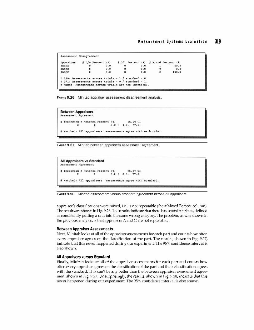
appraiser's classifications were mixed, i.e., is not repeatable (the # Mixed Percent column). The results are shown in Fig. 9.26. The results indicate that there is no consistent bias, defined as consistently putting a unit into the same wrong category. The problem, as was shown in the previous analysis, is that appraisers A and C are not repeatable.

Between Appraiser Assessments Next, Minitab looks at all of the appraiser assessments for each part and counts how often every appraiser agrees on the classification of the part. The results, shown in Fig. 9.27, indicate that this never happened during our experiment. The 95% confidence interval is also shown.

All Appraisers versus Standard Finally, Minitab looks at all of the appraiser assessments for each part and counts how often every appraiser agrees on the classification of the part and their classification agrees with the standard. This can't be any better than the between appraiser assessment agreement shown in Fig. 9.27. Unsurprisingly, the results, shown in Fig. 9.28, indicate that this never happened during our experiment. The 95% confidence interval is also shown.

attribute measurement error analysis -...

Documents