AUDocker LE v1.0

Manual

Team:

Dr M Muralikrishna Kumar, College of Pharmaceutical Sciences, Andhra University

G.Sandeep, Vignan’s Institute of Information Technology, Visakhapatnam

K.Purna Nagasree, College of Pharmaceutical Sciences, Andhra University

Introduction:

Virtual screening is a powerful tool for the discovery of useful ligand molecules out of a given

database of molecules. Vina is an excellent program available for performing docking

simulations (flexible or rigid) on a given protein and ligands. Though the importance of the

computational tools in Medicinal Chemistry was realized by many, very few could successfully

implement it because of lack of knowledge on programming language or computational

facilities. AUDocker LE is designed to help user to perform virtual screening of a large library of

molecules on to a predefined protein/s. It also helps the user to find out the best ligands in the

large dataset used.

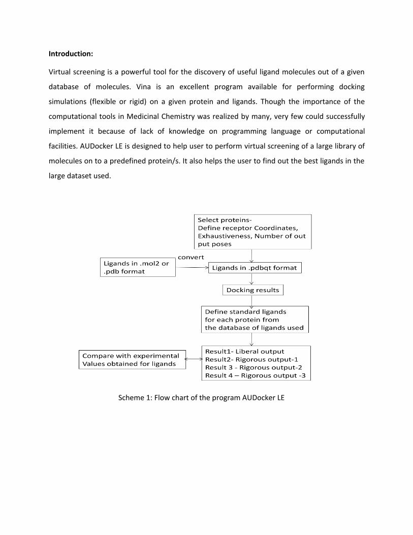
Scheme 1: Flow chart of the program AUDocker LE

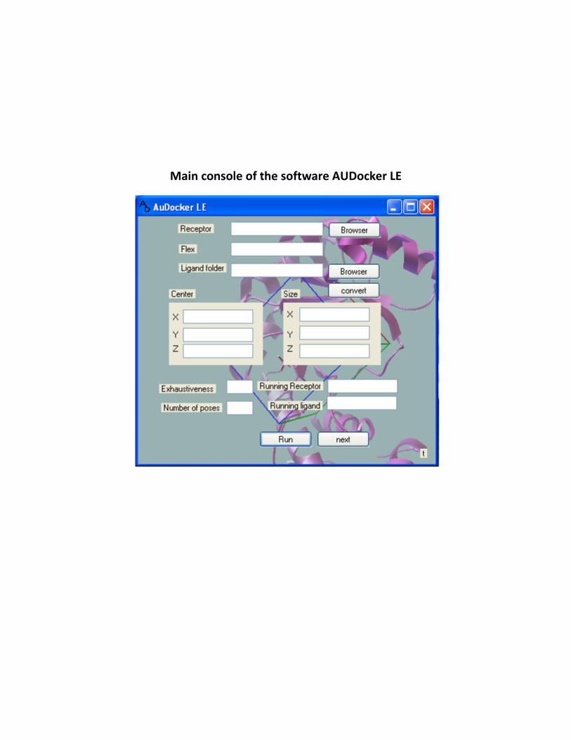
Main console of the software AUDocker LE

Step 1: Selection of proteins

a) Click on the browse button against “Receptor”. This will open a pop-up window, via which

you can select the folder containing test proteins.

b) Pop-up windows (add value) will be opened for the data entry of each protein. Here for each

protein the receptor information, viz coordinates center_x; center_y; center_z and size_x;

size_y; size_z can be entered along with required exhaustiveness and number of output poses.

In this same window you can provide the flex file for your selected protein. (You may keep your

flex protein anywhere)

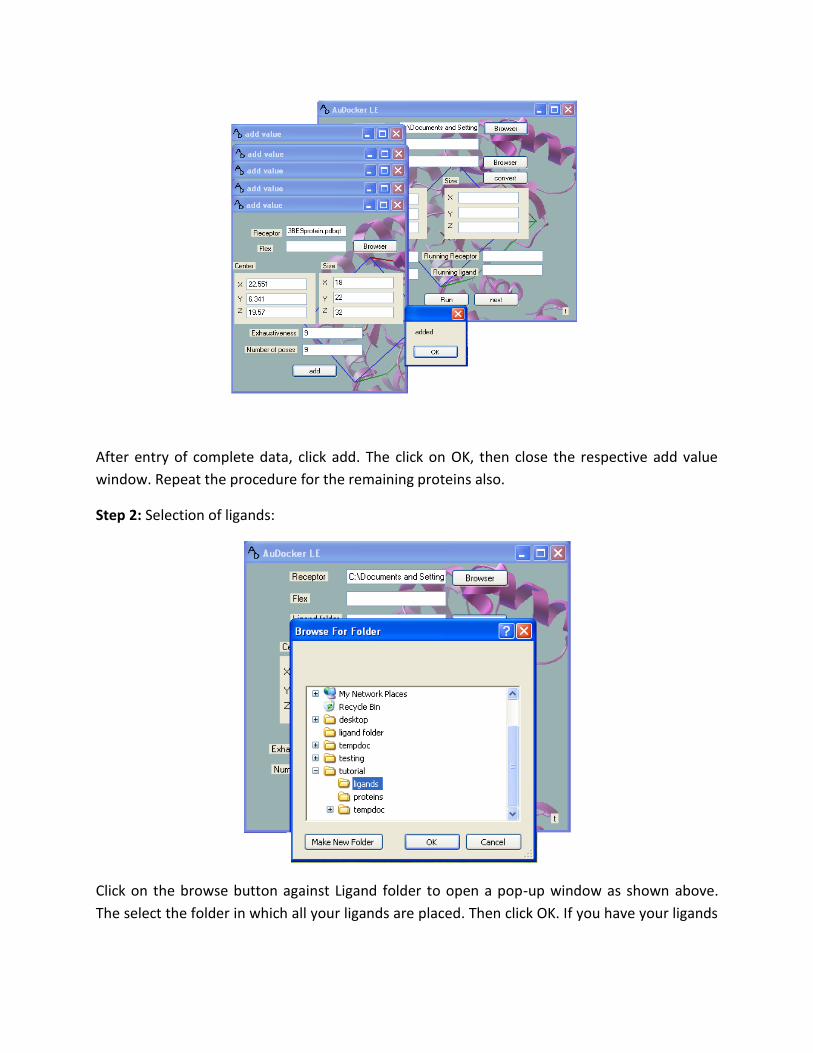
After entry of complete data, click add. The click on OK, then close the respective add value

window. Repeat the procedure for the remaining proteins also.

Step 2: Selection of ligands:

Click on the browse button against Ligand folder to open a pop-up window as shown above.

The select the folder in which all your ligands are placed. Then click OK. If you have your ligands

in either .mol2 or .pdb or a mix of these two then first click the tab “convert” to open the pop-

up window named “convert form”.

From here click the browse button to select the folder containing your ligands the click “ok”.

Then click convert. Wait till the task is completed. Progress of the conversion process may be

seen in “present file converting” text box. After this step you may proceed normally towards

ligand folder selection step.

Step 3: Click “Run” to initiate docking. You may see the progress of the docking may be

monitored in the text boxes given against “Running Receptor” and Running ligand”. Wait till the

pop-up window “completed” appears on the screen.

Step 4: Analysis of the results:

After the successful completion of the docking experiment, Click “Next” on the main console.

Which opens a window named “Standard”. Then click browse to select the protein folder again.

Then pop-up windows named “add standards” will appear on the screen.

Here, you may browse to select the ligand which can be considered as a standard for the

respective protein. For example, if one of the protein we are using for docking is COX-2, and if it

has celecoxib as a co-crystallized ligand, then we may consider this as a standard ligand. You

may also select any other ligand as a standard ligand. The user needs to have prior knowledge

on the bioactivity profile of the ligand which is to be selected as a standard ligand.

+++ Standard ligand must be a part of the database being used for virtual screening+++.

If the user is docking a large database for virtual screening then the standard ligand must be

added to the database before initiating the docking process.

After selection of a standard ligand for each of the target protein, click “Run” and wait till the

pop-up window “Completed” appears on the screen.

Step 5: Open the folder named ‘tempdoc’ in the C-drive, to see the following folders

1) A folder in the name of protein – contains all .txt files generated during docking for that

respective protein.

2) A folder in the name of proteinout – contains all poses files generated during docking for

that respective protein.

3) Three folders named result1, result 2, result 3 and result 4. Which were generated after

processing the results for all the proteins.

The Result 1 folder contains txt files in the name of every protein containing ligands better than

the standard ligand via Ligand Efficiency analysis.

The folders Result 2 and Result 3 contains files in the name of proteins for which good ligands

were obtained via a more rigorous process (LE and normalization of the results).

The folder Result 4 contains files in the name of the proteins containing ligands having the

ligand efficiency greater than m+3σ (Normalization).

All the values which are ≥ m+3σ

Where

m = the average of all the dock scores obtained for the respective protein.

σ = standard deviation in that row.

Normalization procedure:

V = Vo/(Sr+Sc)/2

Where

V = New dock score value

Vo = Old score value

Sc = Average score value obtained for all the ligands for the respective protein (Column)

Sr = Average score values obtained for the respective ligand in all the proteins (Row)

This procedure was tried successfully for virtual screening and more details can be found in the

following references.

Andrew L. Hopkins, Colin R. Groom* and Alexander Alex in DDT Vol. 9, No. 10 May 2004, 430-431. Abad-Zapatero, C.; Metz, J. T. in DDT Vol 10 2005, 464–469. Gianluigi Lauro†, Adriana Romano†, Raffaele Riccio, and Giuseppe Bifulco in J. Nat. Prod., 2011, 74 (6), pp 1401–1407. Step 6: The user may find all the values including Dock scores and the results obtained after the

analysis in a database file named “results.mdb” placed in the C-drive. After completion of

the experiment it is necessary for the user to copy the results in the tempdoc folder and the

results.mdb into appropriately named folder, because these values will be deleted before

the start of a new experiment.

The dock scores which were in the table may be exported to excel for further work.

++ If any of the ligand not docked in the receptor it will be eliminated from the study and kept

in the folder named “not docked” in the tempdoc folder+++

Virtual screening on more number of computers:

In case of handling larger databases and more number of protein targets, the user may let the

docking to go on different machines. If you have 10 proteins and 10,000 molecules for docking,

then let the docking to run on 10 different computers.

Remember that the ligand folder must contain all ligands, including standard ligands for every

protein (if you have 10 proteins you will have to keep 10 standard ligands).

Then copy the contents of the ‘tempdoc’ folder, which contains protein, proteinout and grid

parameter files (as protein.txt), onto a folder on the desktop of any computer.

The data obtained from 10 different computers can now be used for analysis.

Keep all the proteins in a single folder and ligands in another folder.

Perform the step 1: you need not enter the grid parameters and cancel the protein data forms.

Then perform step 2: select the ligand folder.

Click on ‘t’ that was present on the right side corner of the main console to create a table.

By clicking on ‘t’ an button appears on the main console “create table”.

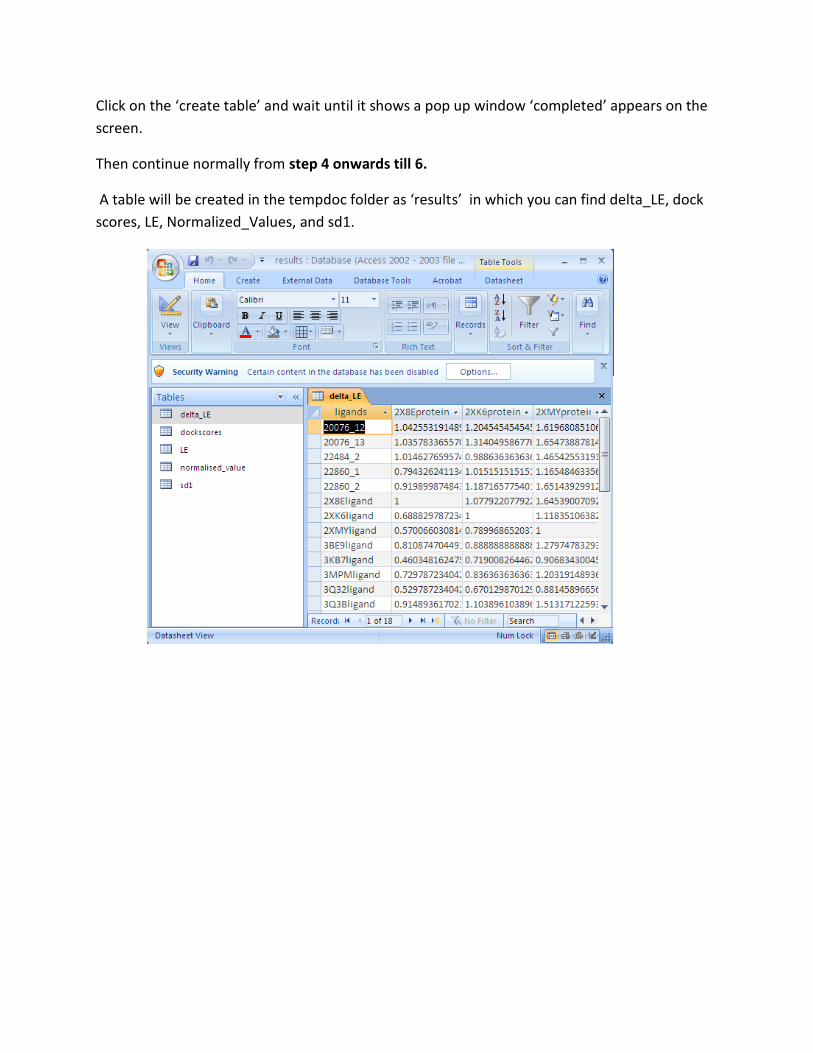
Click on the ‘create table’ and wait until it shows a pop up window ‘completed’ appears on the

screen.

Then continue normally from step 4 onwards till 6.

A table will be created in the tempdoc folder as ‘results’ in which you can find delta_LE, dock

scores, LE, Normalized_Values, and sd1.