Vernay, D.G., Raphael, B. and Smith, I.F.C. "Augmenting simulations of airflow around buildings using field measurements" Advanced Engineering Informatics, 2014, pp 412-424 DOI:10.1016/j.aei.2014.06.003 AUGMENTING SIMULATIONS OF AIRFLOW AROUND BUILDINGS 1

USING FIELD MEASUREMENTS 2

Didier G. Vernay a,c,*, Benny Raphael b and Ian F.C. Smith a,c 3

a) Future Cities Laboratory, ETH Zurich, Zurich, Switzerland. 4 b) Civil Engineering Department, Indian Institute of Technology, Madras, India. 5 c) Applied Computing and Mechanics Laboratory, School of Architecture, Civil and Environmental Engineering (ENAC), 6 EPFL, Lausanne, Switzerland. 7 * Corresponding author: Didier G. Vernay, Future Cities Laboratory, Singapore-ETH Centre 1 CREATE Way #06-01 8 CREATE Tower Singapore 138602. Tel.: +65 9723 1127, E-mail: didier.vernay@epfl.ch 9

Abstract – Computational fluid-dynamics (CFD) simulations have become an important tool for the 10 assessment of airflow in urban areas. However, large discrepancies may appear when simulated 11 predictions are compared with field measurements because of the complexity of airflow behaviour 12 around buildings and difficulties in defining correct sets of parameter values, including those for inlet 13 conditions. Inlet conditions of the CFD model are difficult to estimate and often the values employed 14 do not represent real conditions. In this paper, a model-based data-interpretation framework is proposed 15 in order to integrate knowledge obtained through CFD simulations with those obtained from field 16 measurements carried out in the urban canopy layer (UCL). In this framework, probability-based inlet 17 conditions of the CFD simulation are identified with measurements taken in the UCL. The framework 18 is built on the error-domain model falsification approach that has been developed for the identification 19 of other complex systems. System identification of physics-based models is a challenging task because 20 of the presence of errors in models as well as measurements. This paper presents a methodology to 21 estimate modelling errors. Furthermore, error-domain model falsification has been adapted for the 22 application of airflow modelling around buildings in order to accommodate the time variability of 23 atmospheric conditions. As a case study, the framework is tested and validated for the predictions of 24 airflow around an experimental facility of the Future Cities Laboratory, called “BubbleZERO”. Results 25 show that the framework is capable of narrowing down parameter-value sets from over five hundred to 26 a few having possible inlet conditions for the selected case-study. Thus the case-study illustrates an 27 approach to identifying time-varying inlet conditions and predicting wind characteristics at locations 28 where there are no sensors. 29

Keywords: Computational Fluid Dynamics (CFD); airflow modelling; field measurements; system 30 identification; multi-model reasoning 31

1) INTRODUCTION 32

Urban populations are growing and therefore, understanding urban climate behaviour has become an 33 increasingly important research field. Urban climate has an impact on the comfort and health of 34 residents. The energy consumption of buildings is influenced by the convective heat flux at the building 35 façade and therefore by the wind pattern around buildings (Defraeye et al., 2011). Furthermore, energy 36 demand of buildings can also be reduced by harnessing airflow for natural ventilation (Ghiaus and 37 Allard, 2005). Therefore, cities and buildings should be planned and designed according to 38 characteristics of their climatic environments. 39

Computational fluid-dynamics (CFD) simulations have increasingly been used to simulate the airflow 40 in urban areas (Al-Sallal and Al-Rais, 2011; Van Hooff and Blocken, 2010). CFD simulations 41 numerically solve the fluid-flow equations of motion. In general, the equations are time dependent; this 42

2

means that flow variables at each point have to be computed at several points in time. Directly solving 43 the equations using numerical methods take much computer memory and time and therefore, 44 simplifications are made to mathematical models. In steady Reynolds-averaged Navier-Stokes (RANS)-45 based models, the fluid-flow equations of motion are averaged over time. This results in steady-state 46 equations that are easier to solve. Standard k-epsilon and revised k-epsilon models are examples of 47 RANS-based models. In these models, two additional transport equations are employed to model 48 turbulent properties of the flow. For example, in the standard k-epsilon model, the new transported 49 variables are the turbulent kinetic energy (𝑘𝑘) and turbulent dissipation rate (𝜀𝜀). Another popular 50 approach for modelling turbulence is Large Eddy Simulation (LES) in which time-dependent variations 51 of flow quantities are computed. LES solves large eddies of flow and model the small eddies with a 52 subgrid-scale model. While, this is computationally more efficient than direct numerical solution, it 53 takes significantly greater computation time than RANS-based models. 54

CFD simulations provide high-spatial resolution of data and allow efficient parametric studies for 55 evaluating design configurations (Van Hooff and Blocken, 2010). Due to the increased use of CFD 56 simulations for urban airflow modelling, several sets of best practice guidelines (BPG) have been 57 established (Franke et al., 2011; Tominaga et al., 2008b). However, the accuracy of CFD simulations 58 remains a major concern due to uncertainties associated with i) modelling complex phenomena present 59 in urban environments (Allegrini et al., 2013; Mochida and Lun, 2008; Murakami, 2006), ii) the 60 representation of complex geometrical structures of urban sites and iii) numerical challenges at wall 61 boundaries (Blocken et al., 2007). Even a sophisticated model may not be accurate because of 62 uncertainties in input parameter values such as inlet conditions. For a steady-state model, other 63 significant sources of uncertainties are associated with the time variability of atmospheric conditions 64 (Schatzmann and Leitl, 2011). CFD simulations are thus often validated only with wind-tunnel 65 experiments under controlled experimental conditions (e.g. Ramponi and Blocken, 2012). However, 66 time variability of atmospheric conditions cannot be captured in a conventional wind tunnel in which 67 fixed inlet conditions are employed. In urban environments, many combinations of values of variables 68 such as wind speed, wind direction and turbulent kinetic energy may occur upstream of the area of 69 interest over a short period. The time variability of atmospheric conditions may be estimated using 70 Large Eddy Simulation (LES) with time-dependent inlet conditions. Jiang and Chen found better results 71 using LES with varying wind directions at the inlet rather than using LES with fixed wind directions 72 (Jiang and Chen, 2002). However, LES was only performed during a real-time period of 10-20 min 73 with specific inlet conditions. 74

Challenges appear if field measurements are used to validate steady-state models (Schatzmann and 75 Leitl, 2011). The averaging period of measurement data should be short enough in order to capture the 76 variations at the inlet of the computational domain. However, if a short averaging period is employed, 77 errors between predicted and measured values are expected because of the stochastic time variations of 78 flow characteristics due to low frequency turbulence (Schatzmann and Leitl, 2011). 79

Alternatively, field measurements are employed in order to quantify the airflow in urban areas. 80 Measurement values in the Urban Canopy Layer (UCL) depend on the location of the sensor because 81 of high spatial variability of airflow. Significant variations might be observed if measurements are 82 carried out even a few meters apart from each other (Schatzmann and Leitl, 2011). Therefore, field 83 measurements cannot provide the whole image of the airflow pattern as CFD simulations can do. 84

Model-based data-interpretation strategies have the potential to improve the accuracy of CFD 85 simulations using knowledge obtained from field measurements. In this paper, use of these approaches 86 involves generating sets of CFD simulations through assigning values of parameters that are not known 87 precisely to a model class (template model). 88

3

Many approaches exist for the identification of physics-based models using measurements. 89 Deterministic approaches, in which an optimum model is found by minimizing the differences between 90 model predictions and measurements, may not be appropriate to identify parameter values within model 91 classes because many combinations of parameter values may be consistent with the measurement data. 92 Such ambiguities are amplified by uncertainties in models and measurements, particularly when there 93 are several sources of systematic bias. Modelling assumptions often introduce bias. 94

Moreover, deterministic approaches do not usually provide information on the uncertainties of 95 predictions. Probabilistic approaches, in which many plausible models are found, are more appropriate 96 for identification of environmental models. Their performance depends on the knowledge of the error 97 structure (Beven, 2008). The error structure refers to the probability density function of both 98 measurement and modelling error as well as their spatial correlations. Modelling error originates from 99 uncertainty associated with the model class. 100

Model-falsification approaches such as Generalized Likelihood Uncertainty Estimation (GLUE) 101 (Beven, 2008; Beven, 2006) and the error-domain model falsification approach (Goulet et al., 2013; 102 Goulet et al., 2012) may be used to identify parameter values of CFD models where knowledge of 103 modelling error is not known precisely. Error-domain model falsification involves falsification of model 104 instances for which the difference between measured and predicted values is, for any measurement 105 location, larger than an estimate of maximal values of error defined by combining measurement and 106 modelling uncertainties at that location. The term model instance refers to an instantiation of a model 107 class with specific values of parameters. Error-domain model falsification has not yet been applied to 108 time varying contexts such as airflow around buildings. 109

The first objective of this paper is to present a model-based data interpretation framework that is 110 appropriate for CFD simulations in urban areas. More specifically, a systematic approach for 111 determining ranges of possible inlet conditions is described along with a methodology for estimating 112 modelling errors. In this framework, error-domain model falsification is employed and adapted in order 113 to deal with the time variability of airflow. Modelling errors are estimated by comparing responses of 114 simulations using RANS-based model with those of LES. Responses of LES are not perfectly correct. 115 Therefore, only lower bound estimates of modelling errors are determined in this paper. The second 116 objective is to illustrate this framework using a case study of the “BubbleZERO” facility. 117 “BubbleZERO” is an experimental facility of the Future Cities Laboratory, Singapore-ETH Centre for 118 Global Environmental Sustainability located at the National University of Singapore. 119

The structure of the paper is as follows. In the next section, an overview of the accuracy of CFD 120 simulation for the predictions of wind characteristics in urban areas is provided. A model-based data 121 interpretation framework is proposed in Section 3. Section 4 introduces the case study as well as the set 122 of numerical simulations used in the model-based data interpretation framework. In Section 5, the 123 sensor setup for the case study is described. Section 6 presents a methodology to evaluate modelling 124 errors. Section 7 completes the case study by applying the model-based data interpretation framework 125 to measurement and simulation datasets. The paper ends with a discussion of results, limitations and 126 plans for future work. 127

2) SOURCES OF UNCERTAINTIES IN NUMERICAL SIMULATIONS 128

Several studies have evaluated the performance of RANS-based models for prediction of mean flow 129 quantities around buildings. These studies usually compare responses of numerical simulations with 130 wind tunnel experiments. The advantage of wind tunnel experiments for validation of CFD simulations 131 is that values of simulation parameters and boundary conditions are well known. Hence, if numerical 132 errors are negligible, conclusions related to the performance of the turbulence model can be made. An 133

4

extensive validation study was carried out by Yoshie et al. for the development of the Architectural 134 Institute of Japan (AIJ) guidelines (Yoshie et al., 2007). Comparison between simulations using RANS-135 based models and wind tunnel experiments have been performed for four building geometries, 1) 136 Airflow around a single idealized building with ratio length:width:height=1:1:2, 2) Airflow around an 137 idealized high-rise building with ratio length:width:height=1:1:4 surrounded by low-rise buildings, 3) 138 Airflow in the urban area of Niigata in which CAD data were used, 4) Airflow in the urban area of 139 Shinjuku in which CAD data were used. 140

In the study of the airflow around a single idealized building with ratio length:width:height=1:1:2, 141 responses of CFD simulations using the standard k-epsilon model or revised k-epsilon models have 142 been compared with wind tunnel measurements carried out by Meng and Hibi (1998). It was found that 143 predicted values of amplification factor of wind speeds, U/U0, are in good agreement (±10%) with 144 measured values in regions of high wind speeds (U/U0>1). The amplification factor of wind speeds is 145 defined as the ratio between the local wind speed, U, to the wind speed, U0, that would occur without 146 the presence of buildings. However, in low wind speeds regions (U/U0<1), CFD simulations 147 underestimate the amplification factors of wind speeds by a factor 5 or more (Blocken et al., 2011). 148

Revised k-epsilon models provide slightly more accurate responses in regions of high wind speeds but 149 less accurate responses in regions of low wind speeds. The reverse flow on the roof is not reproduced 150 with the standard k-epsilon model while the reverse flow is slightly overestimated with revised k-151 epsilon models (Yoshie et al., 2007). Overestimation of the region of reverse flow in the wake of the 152 building is observed for all RANS-based models. 153

The same measurement data were used by Tominaga et al. (2008a). In this study, measurements were 154 compared with responses of simulations using RANS-based models (standard k-epsilon model and 155 revised k-epsilon models) as well as responses of LES with and without inflow turbulence. The 156 estimation of the size of the reverse-flow region in the wake of the building is improved if LES is 157 employed (Tominaga et al., 2008a). Responses of LES with inflow turbulence were found to be in good 158 agreement with wind tunnel experiments when predicting mean velocity and turbulent kinetic energy 159 in the wake of the building. 160

Yoshie et al. had similar conclusions for the three other building geometries (Yoshie et al., 2007): in 161 regions of high wind speeds, predicted amplification factors of wind speeds are fairly accurate (±10-162 20%). However, large errors in the predictions of amplification factors are observed in regions of low 163 wind speeds (factor 4-5 or more). 164

Blocken and Carmeliet compared responses of simulations using the Realizable k-epsilon model (Shih 165 et al., 1995) (RANS-based model) with sand-erosion wind-tunnel experiments carried out by Beranek 166 (1979) for three configurations of parallel buildings (Blocken and Carmeliet, 2008). A grid-sensitivity 167 analysis has been performed and high-order discretisation schemes were employed in order to reduce 168 numerical errors. The results confirmed that performance of the RANS-based model in the predictions 169 of amplification factors is higher in regions of high wind speeds (±10 % accuracy). Simulations using 170 the RANS-based model significantly underestimate the amplification factor in regions of low wind 171 speeds (factor 4 or more). 172

Incorrect definition of parameter values/inlet conditions may also lead to uncertain predictions of wind 173 characteristics. Inlet conditions of CFD simulations are difficult to estimate. Even if a measurement 174 station is employed to measure the inlet boundary conditions, the measurements may not be 175 representative of the overall conditions at the inlet because of the high spatial variability of wind 176 characteristics in the UCL (Schatzmann and Leitl, 2011). Even above the buildings, spatial variability 177

5

is observed because the airflow is constantly adapting to the change of surface characteristics 178 (Schatzmann and Leitl, 2011). 179

Buildings are modelled with a certain degree of geometrical simplification in CFD simulations. An 180 equivalent roughness is imposed at building surfaces. The equivalent surface roughness of the 181 surrounding buildings is difficult to estimate and may have a strong influence on predictions of wind 182 speeds (Blocken and Persoon, 2009). In a previous study, field measurements have been used in order 183 to estimate the value of the roughness of the surrounding buildings that leads to the best fit (Blocken 184 and Persoon, 2009). However, as mentioned previously, while calibration approaches force matches of 185 model predictions with measurement data at locations of sensors, they may not be accurate at other 186 locations. 187

3) METHODOLOGY 188

3.1) Description of the system variables 189

This Section presents the model-based data-interpretation framework used to identify plausible 190 parameter values of CFD simulations through measurements carried out in the urban canopy layer. The 191 framework is an adaptation of the error-domain model falsification approach developed by Goulet 192 (Goulet et al., 2013; Goulet et al., 2012). 193

The first step is to define the parameters that need to be identified 𝜽𝜽 = [𝜃𝜃1, … , 𝜃𝜃𝑚𝑚𝑚𝑚𝑚𝑚] with measurements 194 y and their prior ranges of values. In this study, boundary conditions such as the inlet wind speed and 195 direction are treated as parameters of the model. Then, a population of model instances 𝑀𝑀(𝜽𝜽𝑗𝑗) is 196 generated through assigning a set of parameter values 𝜽𝜽𝑗𝑗 to a model class 𝑀𝑀 with 𝑗𝑗 ∈ {1, … , 𝑛𝑛𝑚𝑚}, where 197 𝑛𝑛𝑚𝑚 corresponds to the number of model instances generated. 198

When the right set of parameter values 𝜽𝜽∗ = [𝜃𝜃1∗, … ,𝜃𝜃𝑚𝑚𝑚𝑚𝑚𝑚∗] is assigned to the model class 𝑀𝑀, the 199 predictions of the model instance 𝑀𝑀(𝜽𝜽∗) correspond to the real quantity Q plus a modelling error 𝜖𝜖𝑚𝑚𝑚𝑚𝑚𝑚𝑚𝑚𝑚𝑚. 200 Modelling errors are errors associated with the model class 𝑀𝑀 and they cannot be accounted for through 201 varying values of parameters 𝜽𝜽. Furthermore, measurement 𝑦𝑦 is equal to the real quantity Q plus a 202 measurement error 𝜖𝜖𝑚𝑚𝑚𝑚𝑚𝑚𝑚𝑚𝑚𝑚𝑚𝑚𝑚𝑚. This relation is expressed in Eq. (1). 203

𝑀𝑀(𝜽𝜽∗) + 𝜖𝜖𝑚𝑚𝑚𝑚𝑚𝑚𝑚𝑚𝑚𝑚 = Q = y + 𝜖𝜖𝑚𝑚𝑚𝑚𝑚𝑚𝑚𝑚𝑚𝑚𝑚𝑚𝑚𝑚 (1) 204

Therefore, by rearranging the terms of Eq. (1), the difference between a model prediction and 205 measurement is equal to the difference between measurement and modelling errors. This relation is 206 expressed in Eq. (2). 207

𝑀𝑀(𝜽𝜽∗) − y = 𝜖𝜖𝑚𝑚𝑚𝑚𝑚𝑚𝑚𝑚𝑚𝑚𝑚𝑚𝑚𝑚 − 𝜖𝜖𝑚𝑚𝑚𝑚𝑚𝑚𝑚𝑚𝑚𝑚 (2) 208

Modelling error and measurement error are seldom known. Only bounds of plausible values of errors 209 (imprecise probability) can be estimated. 210

Model instances are considered to be candidate models if the residual of the difference between 211 measured and predicted values fall inside the intervals [𝑇𝑇𝑚𝑚𝑚𝑚𝑚𝑚,𝑇𝑇𝑚𝑚𝑚𝑚𝑚𝑚]. Bounds of these intervals are 212 obtained by computing the difference between measurement and modelling errors using elementary 213 rules of interval arithmetic (Moore, 1966). This is expressed in Eq. (3). 214

𝜖𝜖𝑚𝑚𝑚𝑚𝑚𝑚𝑚𝑚𝑚𝑚𝑚𝑚𝑚𝑚 − 𝜖𝜖𝑚𝑚𝑚𝑚𝑚𝑚𝑚𝑚𝑚𝑚 = �𝜖𝜖𝑚𝑚𝑚𝑚𝑚𝑚𝑚𝑚𝑚𝑚𝑚𝑚𝑚𝑚,𝑚𝑚𝑚𝑚𝑚𝑚, 𝜖𝜖𝑚𝑚𝑚𝑚𝑚𝑚𝑚𝑚𝑚𝑚𝑚𝑚𝑚𝑚,𝑚𝑚𝑚𝑚𝑚𝑚� − �𝜖𝜖𝑚𝑚𝑚𝑚𝑚𝑚𝑚𝑚𝑚𝑚,𝑚𝑚𝑚𝑚𝑚𝑚, 𝜖𝜖𝑚𝑚𝑚𝑚𝑚𝑚𝑚𝑚𝑚𝑚,𝑚𝑚𝑚𝑚𝑚𝑚� 215

= �𝜖𝜖𝑚𝑚𝑚𝑚𝑚𝑚𝑚𝑚𝑚𝑚𝑚𝑚𝑚𝑚,𝑚𝑚𝑚𝑚𝑚𝑚 − 𝜖𝜖𝑚𝑚𝑚𝑚𝑚𝑚𝑚𝑚𝑚𝑚,𝑚𝑚𝑚𝑚𝑚𝑚, 𝜖𝜖𝑚𝑚𝑚𝑚𝑚𝑚𝑚𝑚𝑚𝑚𝑚𝑚𝑚𝑚,𝑚𝑚𝑚𝑚𝑚𝑚 − 𝜖𝜖𝑚𝑚𝑚𝑚𝑚𝑚𝑚𝑚𝑚𝑚,𝑚𝑚𝑚𝑚𝑚𝑚� 216

6

= [𝑇𝑇𝑚𝑚𝑚𝑚𝑚𝑚,𝑇𝑇𝑚𝑚𝑚𝑚𝑚𝑚] (3) 217

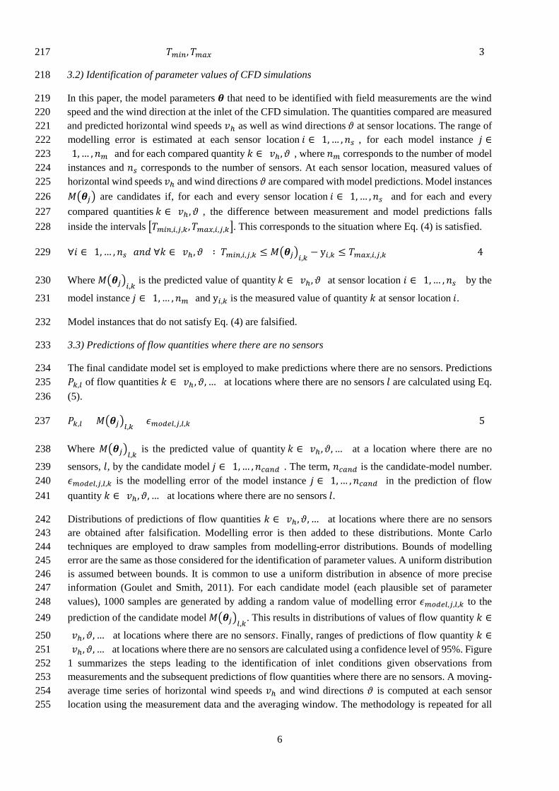
3.2) Identification of parameter values of CFD simulations 218

In this paper, the model parameters 𝜽𝜽 that need to be identified with field measurements are the wind 219 speed and the wind direction at the inlet of the CFD simulation. The quantities compared are measured 220 and predicted horizontal wind speeds 𝑣𝑣ℎ as well as wind directions 𝜗𝜗 at sensor locations. The range of 221 modelling error is estimated at each sensor location 𝑖𝑖 ∈ {1, … ,𝑛𝑛𝑚𝑚}, for each model instance 𝑗𝑗 ∈222 {1, … ,𝑛𝑛𝑚𝑚} and for each compared quantity 𝑘𝑘 ∈ {𝑣𝑣ℎ,𝜗𝜗}, where 𝑛𝑛𝑚𝑚 corresponds to the number of model 223 instances and 𝑛𝑛𝑚𝑚 corresponds to the number of sensors. At each sensor location, measured values of 224 horizontal wind speeds 𝑣𝑣ℎ and wind directions 𝜗𝜗 are compared with model predictions. Model instances 225 𝑀𝑀�𝜽𝜽𝑗𝑗� are candidates if, for each and every sensor location 𝑖𝑖 ∈ {1, … ,𝑛𝑛𝑚𝑚} and for each and every 226 compared quantities 𝑘𝑘 ∈ {𝑣𝑣ℎ ,𝜗𝜗}, the difference between measurement and model predictions falls 227 inside the intervals �𝑇𝑇𝑚𝑚𝑚𝑚𝑚𝑚,𝑚𝑚,𝑗𝑗,𝑘𝑘,𝑇𝑇𝑚𝑚𝑚𝑚𝑚𝑚,𝑚𝑚,𝑗𝑗,𝑘𝑘�. This corresponds to the situation where Eq. (4) is satisfied. 228

∀𝑖𝑖 ∈ {1, … ,𝑛𝑛𝑚𝑚} 𝑎𝑎𝑛𝑛𝑎𝑎 ∀𝑘𝑘 ∈ {𝑣𝑣ℎ,𝜗𝜗} ∶ 𝑇𝑇𝑚𝑚𝑚𝑚𝑚𝑚,𝑚𝑚,𝑗𝑗,𝑘𝑘 ≤ 𝑀𝑀�𝜽𝜽𝑗𝑗�𝑚𝑚,𝑘𝑘 − y𝑚𝑚,𝑘𝑘 ≤ 𝑇𝑇𝑚𝑚𝑚𝑚𝑚𝑚,𝑚𝑚,𝑗𝑗,𝑘𝑘 (4) 229

Where 𝑀𝑀�𝜽𝜽𝑗𝑗�𝑚𝑚,𝑘𝑘 is the predicted value of quantity 𝑘𝑘 ∈ {𝑣𝑣ℎ,𝜗𝜗} at sensor location 𝑖𝑖 ∈ {1, … ,𝑛𝑛𝑚𝑚} by the 230

model instance 𝑗𝑗 ∈ {1, … ,𝑛𝑛𝑚𝑚} and y𝑚𝑚,𝑘𝑘 is the measured value of quantity 𝑘𝑘 at sensor location 𝑖𝑖. 231

Model instances that do not satisfy Eq. (4) are falsified. 232

3.3) Predictions of flow quantities where there are no sensors 233

The final candidate model set is employed to make predictions where there are no sensors. Predictions 234 𝑃𝑃𝑘𝑘,𝑚𝑚 of flow quantities 𝑘𝑘 ∈ {𝑣𝑣ℎ ,𝜗𝜗, … } at locations where there are no sensors 𝑙𝑙 are calculated using Eq. 235 (5). 236

𝑃𝑃𝑘𝑘,𝑚𝑚 = 𝑀𝑀�𝜽𝜽𝑗𝑗�𝑚𝑚,𝑘𝑘 + 𝜖𝜖𝑚𝑚𝑚𝑚𝑚𝑚𝑚𝑚𝑚𝑚,𝑗𝑗,𝑚𝑚,𝑘𝑘 (5) 237

Where 𝑀𝑀�𝜽𝜽𝑗𝑗�𝑚𝑚,𝑘𝑘 is the predicted value of quantity 𝑘𝑘 ∈ {𝑣𝑣ℎ ,𝜗𝜗, … } at a location where there are no 238

sensors, 𝑙𝑙, by the candidate model 𝑗𝑗 ∈ {1, … ,𝑛𝑛𝑐𝑐𝑚𝑚𝑚𝑚𝑚𝑚}. The term, 𝑛𝑛𝑐𝑐𝑚𝑚𝑚𝑚𝑚𝑚 is the candidate-model number. 239 𝜖𝜖𝑚𝑚𝑚𝑚𝑚𝑚𝑚𝑚𝑚𝑚,𝑗𝑗,𝑚𝑚,𝑘𝑘 is the modelling error of the model instance 𝑗𝑗 ∈ {1, … ,𝑛𝑛𝑐𝑐𝑚𝑚𝑚𝑚𝑚𝑚} in the prediction of flow 240 quantity 𝑘𝑘 ∈ {𝑣𝑣ℎ,𝜗𝜗, … } at locations where there are no sensors 𝑙𝑙. 241

Distributions of predictions of flow quantities 𝑘𝑘 ∈ {𝑣𝑣ℎ,𝜗𝜗, … } at locations where there are no sensors 242 are obtained after falsification. Modelling error is then added to these distributions. Monte Carlo 243 techniques are employed to draw samples from modelling-error distributions. Bounds of modelling 244 error are the same as those considered for the identification of parameter values. A uniform distribution 245 is assumed between bounds. It is common to use a uniform distribution in absence of more precise 246 information (Goulet and Smith, 2011). For each candidate model (each plausible set of parameter 247 values), 1000 samples are generated by adding a random value of modelling error 𝜖𝜖𝑚𝑚𝑚𝑚𝑚𝑚𝑚𝑚𝑚𝑚,𝑗𝑗,𝑚𝑚,𝑘𝑘 to the 248 prediction of the candidate model 𝑀𝑀�𝜽𝜽𝑗𝑗�𝑚𝑚,𝑘𝑘. This results in distributions of values of flow quantity 𝑘𝑘 ∈249

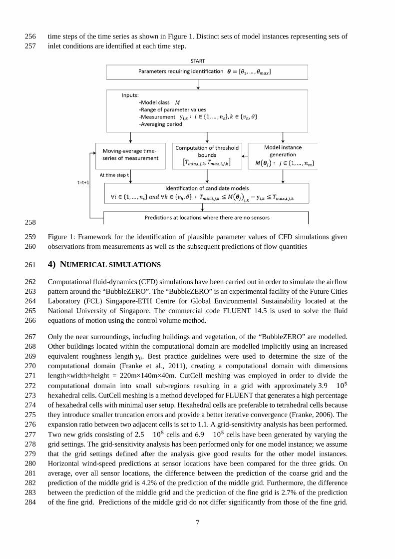
{𝑣𝑣ℎ,𝜗𝜗, … } at locations where there are no sensor𝑠𝑠. Finally, ranges of predictions of flow quantity 𝑘𝑘 ∈250 {𝑣𝑣ℎ,𝜗𝜗, … } at locations where there are no sensors are calculated using a confidence level of 95%. Figure 251 1 summarizes the steps leading to the identification of inlet conditions given observations from 252 measurements and the subsequent predictions of flow quantities where there are no sensors. A moving-253 average time series of horizontal wind speeds 𝑣𝑣ℎ and wind directions 𝜗𝜗 is computed at each sensor 254 location using the measurement data and the averaging window. The methodology is repeated for all 255

7

time steps of the time series as shown in Figure 1. Distinct sets of model instances representing sets of 256 inlet conditions are identified at each time step. 257

258

Figure 1: Framework for the identification of plausible parameter values of CFD simulations given 259 observations from measurements as well as the subsequent predictions of flow quantities 260

4) NUMERICAL SIMULATIONS 261

Computational fluid-dynamics (CFD) simulations have been carried out in order to simulate the airflow 262 pattern around the “BubbleZERO”. The “BubbleZERO” is an experimental facility of the Future Cities 263 Laboratory (FCL) Singapore-ETH Centre for Global Environmental Sustainability located at the 264 National University of Singapore. The commercial code FLUENT 14.5 is used to solve the fluid 265 equations of motion using the control volume method. 266

Only the near surroundings, including buildings and vegetation, of the “BubbleZERO” are modelled. 267 Other buildings located within the computational domain are modelled implicitly using an increased 268 equivalent roughness length 𝑦𝑦0. Best practice guidelines were used to determine the size of the 269 computational domain (Franke et al., 2011), creating a computational domain with dimensions 270 length×width×height = 220m×140m×40m. CutCell meshing was employed in order to divide the 271 computational domain into small sub-regions resulting in a grid with approximately 3.9 × 105 272 hexahedral cells. CutCell meshing is a method developed for FLUENT that generates a high percentage 273 of hexahedral cells with minimal user setup. Hexahedral cells are preferable to tetrahedral cells because 274 they introduce smaller truncation errors and provide a better iterative convergence (Franke, 2006). The 275 expansion ratio between two adjacent cells is set to 1.1. A grid-sensitivity analysis has been performed. 276 Two new grids consisting of 2.5 × 105 cells and 6.9 × 105 cells have been generated by varying the 277 grid settings. The grid-sensitivity analysis has been performed only for one model instance; we assume 278 that the grid settings defined after the analysis give good results for the other model instances. 279 Horizontal wind-speed predictions at sensor locations have been compared for the three grids. On 280 average, over all sensor locations, the difference between the prediction of the coarse grid and the 281 prediction of the middle grid is 4.2% of the prediction of the middle grid. Furthermore, the difference 282 between the prediction of the middle grid and the prediction of the fine grid is 2.7% of the prediction 283 of the fine grid. Predictions of the middle grid do not differ significantly from those of the fine grid. 284

8

Larger differences are observed between predictions of the coarse grid and predictions of the middle 285 grid. Therefore, the middle grid has been selected. 286

The SIMPLE algorithm is employed to deal with the pressure-velocity coupling (Patankar and Spalding, 287 1972). The second-order discretization scheme is used to interpolate pressure from the values obtained 288 at cell centres. The convergence criteria are based on the scaled residuals for all variables, which are 289 set to 10-4. Complexity of trees is reduced by using a tree-canopy model. Trees are modelled using a 290 porous zone (Guo and Maghirang, 2012) defined by a level of porosity of 1 and an isotropic inertial 291 resistance of 0.1m-1. Isothermal simulations were performed. This can be justified due to the cloudy 292 conditions following rain that occurred during the measurement period. The 3D steady RANS equations 293 in combination with the Realizable k-epsilon model have been used to model the turbulent airflow. 294

Vertical profiles of mean wind speed U, turbulent kinetic energy k and turbulence dissipation rate ε are 295 imposed at the inlet of the computational domain using a user-defined function (UDF) in FLUENT. The 296 flow conditions at the inlet of the computational domain are described in Eq. (6), Eq. (7) and Eq. (8) 297 which have been derived from neutral atmospheric conditions. 298

𝑈𝑈(𝑦𝑦) =𝑢𝑢𝐴𝐴𝐴𝐴𝐴𝐴∗

𝜅𝜅ln �

𝑦𝑦 + 𝑦𝑦0𝑦𝑦0

� (6) 299

𝑘𝑘(𝑦𝑦) =𝑢𝑢𝐴𝐴𝐴𝐴𝐴𝐴∗ 2

�𝐶𝐶𝜇𝜇 (7) 300

𝜀𝜀(𝑦𝑦) =𝑢𝑢𝐴𝐴𝐴𝐴𝐴𝐴∗ 3

𝜅𝜅(𝑦𝑦 + 𝑦𝑦0) (8) 301

where 𝑦𝑦 is the height coordinate, 𝜅𝜅 is the von Karman constant, uABL∗ is the atmospheric boundary layer 302 (ABL) friction velocity and Cµ is a model constant. 303

The standard-wall function is used to treat the near-wall behaviour of airflow (Launder and Spalding, 304 1974). A non-dimensional wall distance 𝑦𝑦+ > 30 is achieved at all computational nodes adjacent to 305 wall surfaces as recommended by Franke et al. (2011). In FLUENT, the sand-grain roughness 𝑘𝑘𝑚𝑚 is 306 employed to describe the surface roughness. For the standard wall function implemented in FLUENT, 307 a relationship between 𝑘𝑘𝑚𝑚 and the roughness length 𝑦𝑦0 (commonly used in wind-engineering problems) 308 has been established by Blocken et al. (2007). This relation is expressed in Eq. (9). 309

𝑘𝑘𝑚𝑚 =9.793𝑦𝑦0𝐶𝐶𝑚𝑚

(9) 310

where 𝐶𝐶𝑚𝑚 is the roughness constant. In FLUENT, the value of 𝑘𝑘𝑚𝑚 cannot be larger than 𝑦𝑦𝑝𝑝, which is the 311 distance between the centroid of the wall-adjacent cell and the wall. 312

The roughness length 𝑦𝑦0 of the atmospheric boundary layer with implicitly modelled buildings is set to 313 𝑦𝑦0 = 0.45𝑚𝑚, which represent dense, low buildings (Wieringa, 1992). Therefore, values of sand-grain 314 roughness and roughness constant have been set to 𝑘𝑘𝑚𝑚 = 0.73𝑚𝑚 and 𝐶𝐶𝑚𝑚 = 6 in FLUENT. The roughness 315 length imposed at the ABL surface is the same as the roughness length used to compute the inlet wind 316 profiles in order to avoid stream gradient due to roughness modification in the upstream part of the 317 computational domain (Blocken et al., 2007). The building surfaces are defined with a zero sand-grain 318 roughness (𝑘𝑘𝑚𝑚 = 0𝑚𝑚). The sides and the top of the computational domain are modelled using symmetry 319 boundary conditions. Hence, zero normal velocity is imposed at the sides and top of the computational 320

9

domain. The outlet of the computational domain was modelled assuming zero pressure boundary 321 conditions. 322

Airflow responses depend upon the inlet conditions of the CFD simulation. In urban areas, 323 representative values of inlet conditions are difficult to estimate or measure (Schatzmann and Leitl, 324 2011). In the model-based data interpretation framework, representative values of inlet conditions are 325 identified from measurements taken in the UCL. The parameters requiring identification θ are the wind 326 direction at the inlet 𝜗𝜗𝑚𝑚𝑚𝑚𝑚𝑚𝑚𝑚𝑖𝑖 as well as the reference wind speed at the inlet at 16m height 𝑈𝑈𝑚𝑚𝑚𝑚𝑟𝑟. A 327 population of model instances 𝑀𝑀�𝜽𝜽𝑗𝑗� are generated through assigning sets of parameter values 𝜽𝜽𝑗𝑗 =328 [𝜗𝜗𝑚𝑚𝑚𝑚𝑚𝑚𝑚𝑚𝑖𝑖,𝑗𝑗, 𝑈𝑈𝑚𝑚𝑚𝑚𝑟𝑟,𝑗𝑗] to a model class 𝑀𝑀. 329

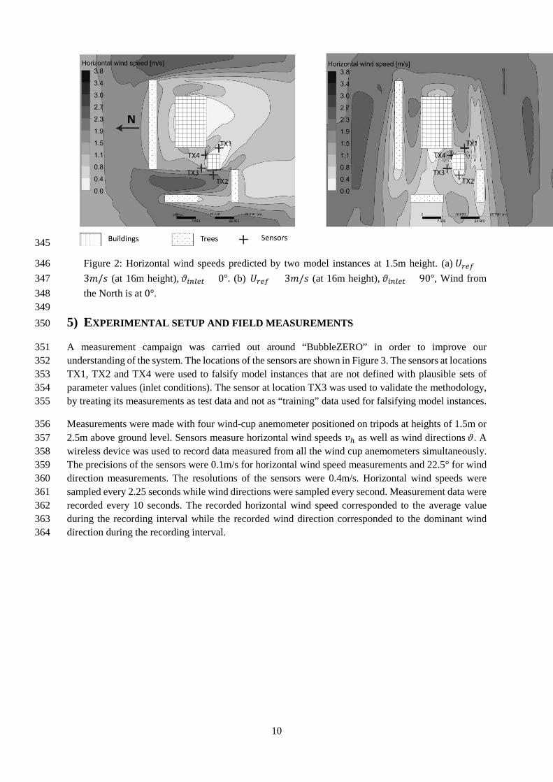
A simple-grid sampling is employed in order to generate model instances uniformly within the 330 parameter space. Table 1 presents the ranges of values of parameter requiring identification as well as 331 their discretization intervals. The simulations were executed using 12 processes in parallel on a 332 Windows Server 2012 containing four Hexa-Core Intel Xeon E54607 2.20GHz processors and 64 GB 333 memory. A total of 504 simulations have been executed in batch mode which requires 48 hours of 334 simulations using FLUENT. The outside box of the computational domain changes its orientation 335 between runs in order to simulate different inlet wind directions 𝜗𝜗𝑚𝑚𝑚𝑚𝑚𝑚𝑚𝑚𝑖𝑖. This leads to the generation of 336 a new grid for each inlet wind direction. For each model instances, horizontal wind speeds 𝑣𝑣ℎ and wind 337 directions 𝜗𝜗 are predicted at sensor locations. Figure 2 presents horizontal wind speeds at 1.5m height 338 predicted with two model instances. Those two model instances are characterized by different wind 339 directions at the inlet 𝜗𝜗𝑚𝑚𝑚𝑚𝑚𝑚𝑚𝑚𝑖𝑖. 340

Table 1: Minimal and maximal bounds of model parameters requiring identification and size of intervals used in the simple-341 grid sampling 342

Parameter requiring identification

Minimal Value

Maximal Value

Discretization intervals

Wind direction at the inlet 𝜗𝜗𝑚𝑚𝑚𝑚𝑚𝑚𝑚𝑚𝑖𝑖 [°] 0 360 10

Reference wind speed at the inlet 𝑈𝑈𝑚𝑚𝑚𝑚𝑟𝑟 (at 16m height) [m/s]

0.5 7 0.5

343

344 a b

10

345

Figure 2: Horizontal wind speeds predicted by two model instances at 1.5m height. (a) 𝑈𝑈𝑚𝑚𝑚𝑚𝑟𝑟 =346 3𝑚𝑚/𝑠𝑠 (at 16m height), 𝜗𝜗𝑚𝑚𝑚𝑚𝑚𝑚𝑚𝑚𝑖𝑖 = 0°. (b) 𝑈𝑈𝑚𝑚𝑚𝑚𝑟𝑟 = 3𝑚𝑚/𝑠𝑠 (at 16m height), 𝜗𝜗𝑚𝑚𝑚𝑚𝑚𝑚𝑚𝑚𝑖𝑖 = 90°, Wind from 347 the North is at 0°. 348 349

5) EXPERIMENTAL SETUP AND FIELD MEASUREMENTS 350

A measurement campaign was carried out around “BubbleZERO” in order to improve our 351 understanding of the system. The locations of the sensors are shown in Figure 3. The sensors at locations 352 TX1, TX2 and TX4 were used to falsify model instances that are not defined with plausible sets of 353 parameter values (inlet conditions). The sensor at location TX3 was used to validate the methodology, 354 by treating its measurements as test data and not as “training” data used for falsifying model instances. 355

Measurements were made with four wind-cup anemometer positioned on tripods at heights of 1.5m or 356 2.5m above ground level. Sensors measure horizontal wind speeds 𝑣𝑣ℎ as well as wind directions 𝜗𝜗. A 357 wireless device was used to record data measured from all the wind cup anemometers simultaneously. 358 The precisions of the sensors were 0.1m/s for horizontal wind speed measurements and 22.5° for wind 359 direction measurements. The resolutions of the sensors were 0.4m/s. Horizontal wind speeds were 360 sampled every 2.25 seconds while wind directions were sampled every second. Measurement data were 361 recorded every 10 seconds. The recorded horizontal wind speed corresponded to the average value 362 during the recording interval while the recorded wind direction corresponded to the dominant wind 363 direction during the recording interval. 364

11

365

Figure 3: Picture of the “BubbleZERO” and position of wind-cup anemometers, TX. 366

Figure 4 presents the moving-average time series of measurements at location TX3 and TX2 using an 367 averaging window of 90 seconds. The moving-average time series are computed by replacing the 368 recorded value (every 10 seconds) with the 90s-averaged value of its neighbour steps. An averaging 369 window of 90 seconds has been employed in this paper. The time variability of horizontal wind speeds 370 is clearly observed in Figure 4. If a longer averaging window is used, the time variability of atmospheric 371 conditions may not have been captured with the proposed model-based data interpretation framework. 372 Measurements were carried out on 18th December 2012 from 1pm to 3pm following rain. Surface 373 heating was negligible due to the cloudy conditions occurring during the measurement campaign. 374

Even though measurements were carried out at locations that are close together, variations of wind 375 quantities are observed between measurement stations. Larger spatial variability of wind quantities 376 might be observed if the measurement stations were located further away from each other. 377

378

Figure 4: Moving-average time series of horizontal wind speed at locations TX3 and TX2 (averaging 379 window of 90 seconds) 380

0 30 60 90 1200

0.5

1

1.5

2

2.5

Time [min]

Hor

izon

tal w

ind

spee

d [m

/s] Location TX3

Location TX2

12

6) MODELLING ERROR 381

An important step that determines the reliability of the identification of parameter values 𝜽𝜽 =382 [𝜗𝜗𝑚𝑚𝑚𝑚𝑚𝑚𝑚𝑚𝑖𝑖 , 𝑈𝑈𝑚𝑚𝑚𝑚𝑟𝑟] is the correct estimation of the threshold bounds �𝑇𝑇𝑚𝑚𝑚𝑚𝑚𝑚,𝑚𝑚,𝑗𝑗,𝑘𝑘 ,𝑇𝑇𝑚𝑚𝑚𝑚𝑚𝑚,𝑚𝑚,𝑗𝑗,𝑘𝑘�, defined by 383 combining measurement and modelling error as expressed in Eq. (3). An estimated range of modelling 384 error in the predictions of horizontal wind speed 𝑣𝑣ℎ and wind direction 𝜗𝜗 is required for each model 385 instance 𝑗𝑗 ∈ {1, … ,𝑛𝑛𝑚𝑚} and at each sensor location 𝑖𝑖 ∈ {1, … ,𝑛𝑛𝑚𝑚} in order to define those bounds. The 386 goal of this Section is to define a relationship between errors associated with a RANS-based model and 387 input/output variables of this model (e.g. errors related to the amplification factor of wind speeds as 388 mentioned in Section 2). 389

Ranges of modelling error have been estimated by comparing responses of CFD simulations obtained 390 with two turbulence models around a single bluff body having dimensions length=6.06m , width=4.88m 391 and height=2.9m which corresponds to the building of interest in the case study presented in Section 4. 392 Dimensions of the computational domain are length×width×height = 55.5m×31.06m×14.5m. The first 393 turbulence model is the same as the one used for the generation of model instances 𝑀𝑀�𝜽𝜽𝑗𝑗�. This 394 turbulence model is built on the steady RANS equations in combination with the Realizable k-epsilon 395 model. The same numerical methods as those described in Section 4 are employed. The second 396 turbulence model is LES using the dynamic Smagorinsky model to model the small eddies of the flow 397 (Germano et al., 1991). Unlike RANS-based model, LES provides time-dependent predictions of flow 398 quantities. LES has been found to be in good agreement with wind tunnel experiments (Cheng et al., 399 2003; Tominaga et al., 2008a) while RANS-based models have difficulties to reproduce flow separation 400 and recirculation because of the unsteadiness of the flow field in those regions. However, since it is 401 computationally prohibitive to perform large numbers of simulations using LES, simulations using a 402 RANS-based model have been employed in the model-based data interpretation framework. Estimates 403 ranges of modelling errors are determined from the differences between responses of LES and responses 404 of the RANS-based model. A grid composed of 7.1 × 104 cells is used for the RANS-based simulation 405 and the LES. A grid-sensitivity analysis has been performed using the RANS-based model in order to 406 define the grid settings, similarly to the analysis performed in Section 4. Scaled residuals of 10-4 for all 407 variables are used as convergence criteria for the RANS-based simulation and the LES. 408

Other sources of error, such as those associated with geometry simplification, have not been considered. 409 Furthermore, LES results are not perfectly correct. Thus, the threshold bounds employed in this paper 410 are lower bound estimates. 411

Profiles of wind speed 𝑈𝑈, turbulent kinetic energy 𝑘𝑘 and turbulent dissipation energy 𝜀𝜀 imposed at the 412 inlet of the RANS-based model are defined using Eq. (6), Eq. (7) and Eq. (8). The ground surface and 413 building surfaces are treated with standard wall functions (Launder and Spalding, 1974) using a zero 414 roughness length (𝑦𝑦0=0m). The inlet wind speed at 1.5m height is used as reference for the definition 415 of the wind speed profile and has been set to 𝑈𝑈1.5𝑚𝑚 = 2𝑚𝑚/𝑠𝑠. The turbulence characteristics defined at 416 the inlet of the RANS-based model are reproduced in LES by imposing a time-dependent inlet velocity 417 profile generated using the vortex method in FLUENT 14.5. Responses of the RANS-based model are 418 used as initial conditions for the LES simulation. A time step size of 0.1 second is used for the LES 419 simulation. After 1 hour of real-time, representative mean values of flow quantities are reached. 420

In Section 6.1, responses of the RANS-based model are compared with mean responses of LES in order 421 to estimate error of RANS-based models in the predictions of mean flow quantities. 422

At each time step of the time series of measurement, measured values at sensor locations are compared 423 with model predictions. Measurements need to be averaged over a short period of time in order to 424

13

capture variation of inlet conditions with the proposed model-based data interpretation framework. In 425 Section 6.2, LES is employed to have an estimate of error associated with fluctuations of flow quantities 426 in which amplitude depends upon the averaging period chosen. In Section 6.3, ranges of errors are 427 estimated for different inlet wind speeds. 428

6.1) Estimated ranges of error in the prediction of mean flow quantities 429

The differences between the mean responses of LES and the responses of the RANS-based model are 430 employed to estimate error of RANS-based models in the predictions of mean flow quantities. 431

Figure 5 presents the spatial distribution of these differences for predictions of mean horizontal wind 432 speeds at 1.5m height. In this study, responses of the RANS-based model have been compared to 433 responses of LES at 1.5m height. This corresponds approximately to half of the height of the building. 434

435

Figure 5: Differences between mean horizontal wind speeds predicted with LES and horizontal wind 436 speeds predicted with the RANS-based model at 1.5m height (wind coming from the right). 437

Figure 6 shows values of differences with respect to the amplification factor of wind speeds U/U0 438 predicted with the RANS-based model at nodes located at 1.5m height. The amplification factor of wind 439 speeds is defined as the ratio between the local horizontal wind speed, U, to the horizontal wind speed, 440 U0, that would occur without buildings. In this study, U0 corresponds to the inlet wind speed at the same 441 height as the local horizontal wind speed U. This assumption is justified because the wind speed profile 442 imposed at the inlet is compatible with the roughness imposed at ground level. Therefore, no stream 443 gradient due to roughness modification in the upstream part of the computational domain is expected. 444 It becomes clear that the range of differences is larger in the region where the amplification factor of 445 wind speeds is less than unity (U/U0<1). 446

Therefore, distinction is made between sensors located in the region of high wind speeds (U/U0>1) and 447 those located in the region of low wind speeds (U/U0<1) in the model-based data interpretation 448 framework. For each region, estimated bounds of error in the predictions of mean horizontal wind 449 speeds are defined as the maximal values of differences observed in the region. Locations of these 450 regions are different for each model instance. Ranges of error at sensor locations, and therefore 451 threshold bounds, are adjusted depending on which region the sensor is located. 452

14

453

Figure 6: Differences between mean horizontal wind speeds predicted with LES and horizontal wind 454 speeds predicted with the RANS-based model at 1.5m; U0=2m/s 455

The same methodology is repeated in order to estimate errors of RANS-based models in the predictions 456 of wind directions. Figure 7 presents differences between mean wind directions predicted with LES and 457 wind directions predicted with the RANS-based model at 1.5m height. In some locations, large 458 differences are observed. This originates from the over-estimation of the region of reverse flow in the 459 wake of the building using RANS-based models. Therefore, RANS-based models may provide a reverse 460 flow at some locations in the wake of the building where LES does not. 461

462

Figure 7: Differences between mean wind directions predicted with LES and wind directions predicted 463 with the RANS-based model at 1.5m height in absolute values 464

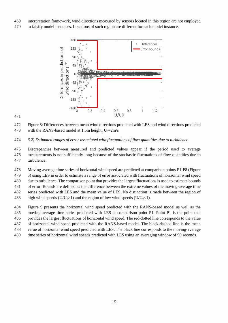
Figure 8 describes values of the differences with respect to the amplification factor of wind speeds 465 U/U0. Large range of differences is observed in the region where the amplification factor of wind speeds 466 is low U/U0<0.33. In this region, the range of difference can be up to [-180°, 180°]. Therefore, sensors 467 located in this region will not add to knowledge of airflow behaviour. In the model-based data-468

0 0.2 0.4 0.6 0.8 1 1.2-0.6

-0.4

-0.2

0

0.2

0.4

0.6

U/U0

Diff

eren

ces i

n pr

edic

tions

of

horiz

onta

l win

d sp

eeds

[m/s

]

Differences Error bounds

15

interpretation framework, wind directions measured by sensors located in this region are not employed 469 to falsify model instances. Locations of such region are different for each model instance. 470

471

Figure 8: Differences between mean wind directions predicted with LES and wind directions predicted 472 with the RANS-based model at 1.5m height; U0=2m/s 473

6.2) Estimated ranges of error associated with fluctuations of flow quantities due to turbulence 474

Discrepancies between measured and predicted values appear if the period used to average 475 measurements is not sufficiently long because of the stochastic fluctuations of flow quantities due to 476 turbulence. 477

Moving-average time series of horizontal wind speed are predicted at comparison points P1-P8 (Figure 478 5) using LES in order to estimate a range of error associated with fluctuations of horizontal wind speed 479 due to turbulence. The comparison point that provides the largest fluctuations is used to estimate bounds 480 of error. Bounds are defined as the difference between the extreme values of the moving-average time 481 series predicted with LES and the mean value of LES. No distinction is made between the region of 482 high wind speeds (U/U0>1) and the region of low wind speeds (U/U0<1). 483

Figure 9 presents the horizontal wind speed predicted with the RANS-based model as well as the 484 moving-average time series predicted with LES at comparison point P1. Point P1 is the point that 485 provides the largest fluctuations of horizontal wind speed. The red-dotted line corresponds to the value 486 of horizontal wind speed predicted with the RANS-based model. The black-dashed line is the mean 487 value of horizontal wind speed predicted with LES. The black line corresponds to the moving-average 488 time series of horizontal wind speeds predicted with LES using an averaging window of 90 seconds. 489

0 0.2 0.4 0.6 0.8 1 1.2-180

-135

-90

-45

0

45

90

135

180

U/U0

Diff

eren

ces

in p

redi

ctio

ns o

f w

ind

dire

ctio

ns [°

]

DifferencesError bounds

16

490

Figure 9: Horizontal wind speed predicted with the RANS-based model at point P1 (red-dotted line), 491 mean horizontal wind speed predicted with LES (black-dashed line) and the moving-average time series 492 of horizontal wind speed predicted with LES (black line); averaging window=90s; U0=2m/s 493

The same methodology is employed to evaluate bounds of error associated with fluctuations of wind 494 directions due to turbulence. Only comparison points characterized by an amplification factor of wind 495 speeds U/U0>0.33 (P3-P8) are considered. In order to deal with the discontinuity of wind direction 496 between 0° and 360°, the average value of wind direction �̅�𝜗 has been determined using Eq. (10). 497

�̅�𝜗 = 𝑎𝑎𝑎𝑎𝑎𝑎𝑛𝑛2(sın𝜗𝜗������, cos𝜗𝜗�������) (10) 498

Where sın𝜗𝜗������ and cos𝜗𝜗������� correspond to the average value of the sine and cosine of the wind direction 𝜗𝜗. 499

It is clear that the maximal fluctuations of flow quantities depend on the averaging window chosen. 500 Figure 10 presents the estimated bounds of error in the predictions of horizontal wind speeds and wind 501 directions with respect to the averaging window. If the averaging window increases, the estimated 502 ranges of error decrease. 503

504

505

0 30 60 90 1200

0.1

0.2

0.3

0.4

0.5

0.6

0.7

0.8

Time [min]

Hor

izon

tal w

ind

spee

d [m

/s]

RANS-based modelMean value of LESMoving-average time series

0 100 200 300 400 500-2

-1.5

-1

-0.5

0

0.5

1

1.5

2

Averaging window [s]

Estim

ated

bou

nds

of e

rror

in th

e

pred

ictio

n of

hor

izon

tal w

ind

spee

d [m

/s]

0 100 200 300 400 500-45

0

45

Averaging window [s]

Estim

ated

bou

nds

of e

rror

in th

e pr

edic

tion

of w

ind

dire

ctio

n [°

]a b

17

506

Figure 10: Estimated bounds of errors associated with the fluctuations of flow quantities due to 507 turbulence with respect to the averaging window. (a) Bounds of error in the predictions of horizontal 508 wind speeds. (b) Bounds of error in the predictions of wind directions; U0=2m/s 509

6.3) Estimated ranges of error for different inlet wind speeds 510

Bounds of modelling error 𝜖𝜖𝑚𝑚𝑚𝑚𝑚𝑚𝑚𝑚𝑚𝑚 are computed by summing the estimated bounds of error of RANS-511 based models in the predictions of mean flow quantities (Section 6.1) with those associated with the 512 fluctuations of flow quantities due to turbulence (Section 6.2). 513

Two sets of simulations with two inlet wind speeds U0 have been executed in order to evaluate the 514 influence of the inlet wind speed on the estimated ranges of modelling error. In order to estimate ranges 515 of error for other inlet wind speeds, a linear interpolation has been assumed. In future work, RANS-516 based models and LES will be compared with other inlet wind speeds in order to better define the 517 relationship between inlet wind speed and ranges of modelling error. 518

Figure 11 presents the estimated ranges of error of RANS-based models in the predictions of mean flow 519 quantities as well as the estimated ranges of error associated with the fluctuations of flow quantities due 520 to turbulence with respect to the inlet wind speed U0. Figure 12a presents the estimated ranges of errors 521 in the predictions of horizontal wind speeds in the region of high wind speeds (U/U0>1). The estimated 522 ranges of errors in the predictions of wind speeds in the region of low wind speeds (U/U0<1) are not 523 represented in this figure. Figure 12b presents the estimated ranges of error in the predictions of wind 524 directions in the region characterized by U/U0>0.33. 525

526

Figure 11: Estimated ranges of modelling errors with respect to the inlet wind speed U0 (averaging 527 window = 90s). (a) Modelling error associated with predictions of wind speeds in the region where 528 U/U0>1. (b) Modelling error associated with predictions of wind directions in the region where 529 U/U0>0.33. 530

7) RESULTS 531

7.1) Identification of inlet conditions 532

a b

18

This Section presents the results of the model-based data interpretation framework using predictions of 533 the model instances (Section 4), the measurement data (Section 5) as well as the knowledge of 534 modelling errors (Section 6). In this framework, a population of model instances 𝑀𝑀�𝜽𝜽𝑗𝑗� is generated 535 through assigning parameter values 𝜽𝜽𝑗𝑗 = [𝜗𝜗𝑚𝑚𝑚𝑚𝑚𝑚𝑚𝑚𝑖𝑖,𝑗𝑗, 𝑈𝑈𝑚𝑚𝑚𝑚𝑟𝑟,𝑗𝑗 ] to a model class 𝑀𝑀. Measurements are 536 employed to falsify model instances that are not defined with plausible sets of parameter values. 537

Measurement errors are determined according to the precision of the sensor (Section 5). Moreover, if 538 the measured value of horizontal wind speed is below the starting threshold of the sensor (0.4m/s), 539 values of measurement errors are adjusted. 540

A study has been performed in order to evaluate errors associated with sensor-location uncertainties. In 541 this study, one model instance has been used. For each sensor location, wind speeds and wind directions 542 are predicted at 100 points located within a distance of 20cm from the sensor location. The maximal 543 differences between predictions at those points and predictions at sensor locations are used to estimate 544 these errors. The maximal range of differences for wind speeds is [-0.069m/s, 0.062m/s] and the 545 maximal range of differences for wind directions is [-3.3°, 2.9°]. These errors have been added to the 546 other sources of errors using elementary rules of interval arithmetic (Equation 3). 547

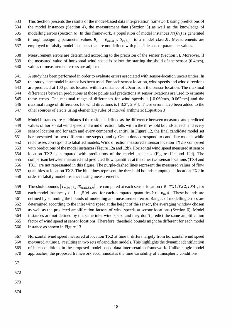
Model instances are candidates if the residual, defined as the difference between measured and predicted 548 values of horizontal wind speed and wind direction, falls within the threshold bounds at each and every 549 sensor location and for each and every compared quantity. In Figure 12, the final candidate model set 550 is represented for two different time steps t1 and t2. Green dots correspond to candidate models while 551 red crosses correspond to falsified models. Wind direction measured at sensor location TX2 is compared 552 with predictions of the model instances (Figure 12a and 12b). Horizontal wind speed measured at sensor 553 location TX2 is compared with predictions of the model instances (Figure 12c and 12d). The 554 comparison between measured and predicted flow quantities at the other two sensor locations (TX4 and 555 TX1) are not represented in this figure. The purple-dashed lines represent the measured values of flow 556 quantities at location TX2. The blue lines represent the threshold bounds computed at location TX2 in 557 order to falsify model instances using measurements. 558

Threshold bounds �𝑇𝑇𝑚𝑚𝑚𝑚𝑚𝑚,𝑚𝑚,𝑗𝑗,𝑘𝑘 ,𝑇𝑇𝑚𝑚𝑚𝑚𝑚𝑚,𝑚𝑚,𝑗𝑗,𝑘𝑘� are computed at each sensor location 𝑖𝑖 ∈ {𝑇𝑇𝑇𝑇1,𝑇𝑇𝑇𝑇2,𝑇𝑇𝑇𝑇4}, for 559 each model instance 𝑗𝑗 ∈ {1, … ,504} and for each compared quantities 𝑘𝑘 ∈ {𝑣𝑣ℎ,𝜗𝜗}. These bounds are 560 defined by summing the bounds of modelling and measurement error. Ranges of modelling errors are 561 determined according to the inlet wind speed at the height of the sensor, the averaging window chosen 562 as well as the predicted amplification factors of wind speeds at sensor locations (Section 6). Model 563 instances are not defined by the same inlet wind speed and they don’t predict the same amplification 564 factor of wind speed at sensor locations. Therefore, threshold bounds might be different for each model 565 instance as shown in Figure 13. 566

Horizontal wind speed measured at location TX2 at time t1 differs largely from horizontal wind speed 567 measured at time t2, resulting in two sets of candidate models. This highlights the dynamic identification 568 of inlet conditions in the proposed model-based data interpretation framework. Unlike single-model 569 approaches, the proposed framework accommodates the time variability of atmospheric conditions. 570

571

572

573

574

19

575

576

577

578

579

Figure 12: Comparison between measured and predicted flow quantities at location TX2. (a) 580 Comparison of wind direction at t1=300s. (b) Comparison of wind direction at t2=1000s. (c) Comparison 581 of horizontal wind speed at t1=300s. (d) Comparison of horizontal wind speed at t2=1000s. 582

Figure 13 presents the final candidate model sets obtained after falsification using measurement taken 583 at locations TX1, TX2 and TX4 represented in the parameter space. Green dots correspond to the final 584 candidate model set obtained at time t1 while the green triangles correspond to the final candidate model 585 set obtained at time t2. Red crosses correspond to the falsified models. It becomes clear that the initial 586 range of parameter values have been reduced through the use of measurement data taken in the UCL. 587 At time t1, the number of candidate models is reduced from 504 to 40. At time t2, the number of 588 candidate models is reduced from 504 to 16. The final candidate model set at time t1 is different from 589 the final candidate model set obtained at time t2. These two final candidate model sets represent very 590

0 100 200 300 400 5000

45

90

135

180

225

270

315

360

Model instances

Win

d di

rect

ion

at T

X2 fr

om N

[°]

t=t1

candidate modelfalsified modelmeasured valuethreshold bounds

0 100 200 300 400 5000

45

90

135

180

225

270

315

360

Model instances

Win

d di

rect

ion

at T

X2 fr

om N

[°]

t=t2

0 100 200 300 400 5000

0.5

1

1.5

2

2.5

3

3.5

4

4.5

Model instances

Hor

izon

tal w

ind

spee

d at

TX2

[m/s

]

t=t1

0 100 200 300 400 5000

0.5

1

1.5

2

2.5

3

3.5

4

4.5

Model instances

Hor

izon

tal w

ind

spee

at T

X2 [m

/s]

t=t2

a b

c d

20

different boundary conditions existing at the selected time steps. It further describes typical time 591 variability of airflow in urban areas. 592

593

Figure 13: Final candidate model set at time t1=300s (green dots) and at time t2=1000s (green triangles) 594 represented in the parameter space 595

Figure 14 presents the number of occurrence of each model instance over time. Each bin represents one 596 model instance. The height of the bin represents the number of occurrences. Model instances with high 597 occurrences represent predominant inlet conditions. 598

599

Figure 14: Number of occurrences of each model instance over time 600

7.2) Predictions of flow quantities where there are no-sensors 601

At each time step (every 10 seconds), the final candidate model set is employed to predict flow 602 quantities where no measurements are carried out. Modelling uncertainty is combined to the distribution 603 of predictions obtained with the final candidate set as explained in Section 3.3. Ranges of predictions 604 are calculated using the uncertainty combination and a confidence level of 95%. 605

0 45 90 135 180 225 270 315 360

1

2

3

4

5

6

7

Wind direction inlet from N [°]

Refe

renc

e w

ind

spee

d in

let [

m/s

]

falsified modelcand. model at time t1cand. model at time t2

21

For validation of the proposed framework, moving-average time series of horizontal wind speeds and 606 wind directions are computed at locations TX3 using the measurement dataset and an averaging window 607 of 90s. At each time step, measured values of horizontal wind speeds and wind directions are compared 608 with ranges of predictions obtained at locations TX3. It is emphasized that measurement data obtained 609 at location TX3 was not used to identify candidate models and was used only to test whether the 610 predictions of flow quantities are reliable. 611

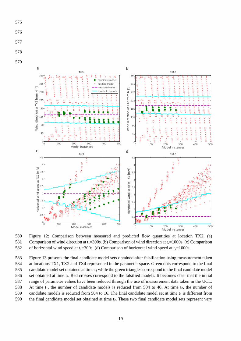
Figure 15a presents ranges of predicted horizontal wind speeds as well as the moving-average time 612 series of horizontal wind speeds measured at location TX3. Figure 15b presents ranges of predicted 613 wind directions as well as the moving-average time series of wind directions measured at location TX3. 614 Only 15 minutes of the measurement dataset are represented in these figures. If we consider the whole 615 measurement campaign (2 hours), horizontal wind speeds measured at location TX3 fall within ranges 616 of predictions 96% of the time. Wind directions fall within ranges of predictions 93% of the time. This 617 demonstrates that predictions of flow quantities using the model-based data-interpretation framework 618 at location TX3 are fairly reliable. 619

Other sources of modelling error such as geometry simplification need to be considered in the model 620 falsification approach in order to improve the reliability of identification and subsequent predictions. 621 Moreover, the modelling errors have been estimated by comparing responses of a RANS-based model 622 with those of LES. Although LES is more accurate than RANS-based in regions of flow separation and 623 recirculation, LES is not an exact representation of reality. Therefore, only lower bound estimates of 624 modelling errors are determined in this paper. 625

Figure 15: Ranges of predictions as well as the moving-average time series of flow quantities at 626 location TX3 (averaging window of 90 seconds) 627

8) DISCUSSION 628

This paper proposed a model-based data interpretation framework for the assessment of airflow in urban 629 areas. In this framework, predictions obtained with CFD simulations are integrated with data obtained 630 with measurements as well as with knowledge of uncertainties in order to improve the accuracy of 631 airflow predictions in urban areas. A systematic approach for the estimation of modelling error 632 associated with RANS-based models has been incorporated to this framework. The results show that 633 predictions in terms of mean wind speeds and mean wind directions are more accurate in regions of 634 high wind speeds (high amplification factor of wind speeds) than in regions of low wind speeds. This 635 is in agreement with recent work by Blocken et al. (2011) on the performance of RANS-based models 636 for airflow modelling using CFD simulations. The framework accommodates the time variability of 637 atmospheric conditions by 1) identifying different sets of boundary conditions at each time step and by 638

0 2 4 6 8 10 12 14 150

0.5

1

1.5

2

2.5

3

3.5

4

Time [min]

Hor

izon

tal w

ind

spee

d at

TX3

[m/s

]

Measured values Bounds of predictions

0 2 4 6 8 10 12 14 150

45

90

135

180

225

270

315

360

Time [min]

Win

d di

rect

ion

at T

X3 [°

]

a b

22

2) adding additional source of errors associated with the fluctuations of flow quantities during the 639 computation of thresholds bounds. 640

There are (of course) limitations. In the present study, only inlet conditions have been identified using 641 measurements taken in the UCL. Other parameters that may influence the airflow around buildings, 642 such as the roughness of the surrounding buildings or the inertial resistance of trees, have not been 643 considered. In further studies, more parameters will be identified that have varying values with respect 644 to time (e.g. inlet conditions) as well as constant values with respect to time (e.g. roughness of 645 buildings). A grid-based sampling has been used for the generation of model instances in this work. In 646 this approach, the size of the initial candidate model set increases exponentially with the number of 647 parameters requiring identification. More efficient techniques may be used in order to decrease the 648 complexity of sampling in high-dimensional parameter space. Moreover, if many parameter values need 649 to be identified, care is needed in order to avoid parameter compensation at sensor locations. 650

CFD simulations have been performed on small-size buildings. Only the “BubbleZERO” and its near-651 surroundings are explicitly modelled. Therefore the computational domain is relatively small 652 (length×width×height=220m×140m×40m). Sensors used in this study are located close to each other 653 and therefore, the spatial variability of airflow is not well-pronounced. In future work, the framework 654 will be tested and validated in a case study with larger computational domain and taller buildings. More 655 sensors will be employed and they will be located further away from each other. 656

In this paper, only modelling errors in the predictions of mean flow quantities using RANS-based 657 models as well as errors associated with fluctuations of flow quantities have been acknowledged. The 658 modelling errors have been defined by comparing responses of a RANS-based model with those of LES 659 around an isolated building with a cubical shape. Although LES is clearly more accurate than RANS-660 based models in the predictions of mean flow characteristics, LES does not perfectly simulate the 661 airflow behaviour around buildings (Lim et al., 2009; Tominaga et al., 2008a). 662

Moreover, in other building configurations, ranges of errors as well as their relationship with the 663 amplification factor of wind speeds or the averaging window may differ from those obtained in the 664 present study. Furthermore, other sources of errors need to be considered in order to predict more 665 reliable ranges of predictions at locations where there are no sensors. Sources include simplifications 666 of urban shapes, idealisation of boundary conditions with a logarithmic profile that has been derived 667 for neutral conditions as well as the assumption that thermal processes, such as convection, are 668 negligible. Also, errors due to values of parameters that are difficult to quantify and that have not been 669 identified, such as the roughness of the surrounding buildings or the inertial resistance of trees, influence 670 reliability. Finally, the proposed methodology used to estimate spatial variations of ranges of modelling 671 errors depending on the predicted amplification factor of wind speeds should help define optimal sensor 672 configurations in further studies. 673

9) CONCLUSIONS 674

This work has led to the following conclusions: 675

1) The model-falsification methodology has much potential for interpreting sensor measurements 676 to improve the accuracy of airflow simulations around buildings. 677

2) Adapting the error-domain model falsification approach to represent the dynamic behaviour of 678 airflow has successfully led to narrowing down several hundred parameter-value sets to a few 679 possible inlet conditions for the selected case-study. Thus the case-study illustrates an approach 680 for identifying time-varying inlet conditions and predicting wind characteristics at locations 681 where there are no sensors. 682

23

3) Modelling errors need to be recognized and quantified in order to perform reliable predictions 683 of airflow characteristics at locations where there are no-sensors. Ranges of modelling errors 684 depend on the predicted amplification factor of wind speeds, the wind speed at the inlet as well 685 as the time period employed to average measurement data. 686

ACKNOWLEDGMENT 687

This work was established at the Singapore-ETH Centre for Global Environmental Sustainability 688 (SEC), co-funded by the Singapore National Research Foundation (NRF) and ETH Zurich. The first 689 author is a registered PhD student at EPFL. The authors would like to thank Prof. C. Sekhar, Prof. M. 690 Santamouris, Dr. J-A. Goulet and M. Papadopoulou for their support. We also thank the anonymous 691 reviewers for their comments. 692

REFERENCES 693

Al-Sallal, K.A., Al-Rais, L., 2011. Outdoor airflow analysis and potential for passive cooling in the 694 traditional urban context of Dubai. Renewable Energy 36 (9), 2494-2501. 695

Allegrini, J., Dorer, V., Carmeliet, J., 2013. Wind tunnel measurements of buoyant flows in street 696 canyons. Building and Environment 59 315-326. 697

Beranek, W., 1979. Beperken van windhinder om gebouwen, deel 2. Deventer: Stichting Bouwresearch 698 no. 90. Kluwer Technische Boeken BV, 699

Beven, K., 2008. Environmental modelling: An uncertain future? Taylor & Francis, 700 Beven, K., 2006. A manifesto for the equifinality thesis. Journal of hydrology 320 (1), 18-36. 701 Blocken, B., Carmeliet, J., 2008. Pedestrian wind conditions at outdoor platforms in a high-rise 702

apartment building: generic sub-configuration validation, wind comfort assessment and 703 uncertainty issues. Wind and Structures 11 (1), 51-70. 704

Blocken, B., Persoon, J., 2009. Pedestrian wind comfort around a large football stadium in an urban 705 environment: CFD simulation, validation and application of the new Dutch wind nuisance 706 standard. Journal of Wind Engineering and Industrial Aerodynamics 97 (5), 255-270. 707

Blocken, B., Stathopoulos, T., Carmeliet, J., 2007. CFD simulation of the atmospheric boundary layer: 708 wall function problems. Atmospheric environment 41 (2), 238-252. 709

Blocken, B., Stathopoulos, T., Carmeliet, J., Hensen, J.L., 2011. Application of computational fluid 710 dynamics in building performance simulation for the outdoor environment: an overview. 711 Journal of Building Performance Simulation 4 (2), 157-184. 712

Cheng, Y., Lien, F., Yee, E., Sinclair, R., 2003. A comparison of large Eddy simulations with a standard 713 k–ε Reynolds-averaged Navier–Stokes model for the prediction of a fully developed turbulent 714 flow over a matrix of cubes. Journal of Wind Engineering and Industrial Aerodynamics 91 (11), 715 1301-1328. 716

Defraeye, T., Blocken, B., Carmeliet, J., 2011. Convective heat transfer coefficients for exterior 717 building surfaces: Existing correlations and CFD modelling. Energy Conversion and 718 Management 52 (1), 512-522. 719

Franke, J., 2006. Recommendations of the COST action C14 on the use of CFD in predicting pedestrian 720 wind environment. In: The fourth international symposium on computational wind engineering, 721 Yokohama, Japan, pp. 529-532. 722

Franke, J., Hellsten, A., Schlunzen, K.H., Carissimo, B., 2011. The COST 732 Best Practice Guideline 723 for CFD simulation of flows in the urban environment: a summary. International Journal of 724 Environment and Pollution 44 (1), 419-427. 725

Germano, M., Piomelli, U., Moin, P., Cabot, W.H., 1991. A dynamic subgrid‐scale eddy viscosity 726 model. Physics of Fluids A: Fluid Dynamics 3 1760. 727

Ghiaus, C., Allard, F., 2005. Natural ventilation in the urban environment: assessment and design. 728 Earthscan, 729

Goulet, J.-A., Coutu, S., Smith, I.F.C., 2013. Model falsification diagnosis and sensor placement for 730 leak detection in pressurized pipe networks. Advanced Engineering Informatics 27 (2), 261-731 269. 732

24

Goulet, J.-A., Michel, C., Smith, I.F.C., 2012. Hybrid probabilities and error-domain structural 733 identification using ambient vibration monitoring. Mechanical Systems and Signal Processing 734 37 (1), 199-212. 735

Goulet, J.-A., Smith, I.F., 2011. Extended uniform distribution accounting for uncertainty of 736 uncertainty. In: International Conference on Vulnerability and Risk Analysis and 737 Management/Fifth International Symposium on Uncertainty Modeling and Analysis, 738 Maryland, USA, pp. 78-85. 739

Guo, L., Maghirang, R.G., 2012. Numerical simulation of airflow and particle collection by vegetative 740 barriers. 741

Jiang, Y., Chen, Q., 2002. Effect of fluctuating wind direction on cross natural ventilation in buildings 742 from large eddy simulation. Building and Environment 37 (4), 379-386. 743

Launder, B.E., Spalding, D., 1974. The numerical computation of turbulent flows. Computer methods 744 in applied mechanics and engineering 3 (2), 269-289. 745

Lim, H.C., Thomas, T., Castro, I.P., 2009. Flow around a cube in a turbulent boundary layer: LES and 746 experiment. Journal of Wind Engineering and Industrial Aerodynamics 97 (2), 96-109. 747

Meng, Y., Hibi, K., 1998. Turbulent measurements of the flow field around a high-rise building. Journal 748 of Wind Engineering 76 55-64. 749

Mochida, A., Lun, I.Y., 2008. Prediction of wind environment and thermal comfort at pedestrian level 750 in urban area. Journal of Wind Engineering and Industrial Aerodynamics 96 (10), 1498-1527. 751

Moore, R.E., 1966. Interval analysis. Prentice-Hall Englewood Cliffs, 752 Murakami, S., 2006. Environmental design of outdoor climate based on CFD. Fluid dynamics research 753

38 (2), 108-126. 754 Patankar, S.V., Spalding, D.B., 1972. A calculation procedure for heat, mass and momentum transfer 755

in three-dimensional parabolic flows. International Journal of Heat and Mass Transfer 15 (10), 756 1787-1806. 757

Ramponi, R., Blocken, B., 2012. CFD simulation of cross-ventilation flow for different isolated 758 building configurations: validation with wind tunnel measurements and analysis of physical 759 and numerical diffusion effects. Journal of Wind Engineering and Industrial Aerodynamics 104 760 408-418. 761

Schatzmann, M., Leitl, B., 2011. Issues with validation of urban flow and dispersion CFD models. 762 Journal of Wind Engineering and Industrial Aerodynamics 99 (4), 169-186. 763

Shih, T.-H., Liou, W.W., Shabbir, A., Yang, Z., Zhu, J., 1995. A new k–ε eddy viscosity model for high 764 reynolds number turbulent flows. Computers & Fluids 24 (3), 227-238. 765

Tominaga, Y., Mochida, A., Murakami, S., Sawaki, S., 2008a. Comparison of various revised k–ε 766 models and LES applied to flow around a high-rise building model with 1: 1: 2 shape placed 767 within the surface boundary layer. Journal of Wind Engineering and Industrial Aerodynamics 768 96 (4), 389-411. 769

Tominaga, Y., Mochida, A., Yoshie, R., Kataoka, H., Nozu, T., Yoshikawa, M., Shirasawa, T., 2008b. 770 AIJ guidelines for practical applications of CFD to pedestrian wind environment around 771 buildings. Journal of Wind Engineering and Industrial Aerodynamics 96 (10), 1749-1761. 772

Van Hooff, T., Blocken, B., 2010. Coupled urban wind flow and indoor natural ventilation modelling 773 on a high-resolution grid: A case study for the Amsterdam ArenA stadium. Environmental 774 Modelling & Software 25 (1), 51-65. 775

Wieringa, J., 1992. Updating the Davenport roughness classification. Journal of Wind Engineering and 776 Industrial Aerodynamics 41 (1), 357-368. 777

Yoshie, R., Mochida, A., Tominaga, Y., Kataoka, H., Harimoto, K., Nozu, T., Shirasawa, T., 2007. 778 Cooperative project for CFD prediction of pedestrian wind environment in the Architectural 779 Institute of Japan. Journal of Wind Engineering and Industrial Aerodynamics 95 (9), 1551-780 1578. 781

This work is licensed under a Creative Commons Attribution-NonCommercial-NoDerivatives 4.0 782 International License 783