august 2015 energy research partnership managing...
TRANSCRIPT

August 2015 Energy Research Partnership
Managing Flexibility Whilst Decarbonising the GB Electricity System

2
»
The Energy Research PartnershipThe Energy Research Partnership is a high-level forum bringing together key stakeholders and funders of energy research, development, demonstration and deployment in Government, industry and academia, plus other interested bodies, to identify and work together towards shared goals.
The Partnership has been designed to give strategic direction to UK energy innovation, seeking to influence the development of new technologies and enabling timely, focussed investments to be made. It does this by (i) influencing members in their respective individual roles and capacities and (ii) communicating views more widely to other stakeholders and decision makers as appropriate. ERP’s remit covers the whole energy system, including supply (nuclear, fossil fuels, renewables), infrastructure, and the demand side (built environment, energy efficiency, transport).
The ERP is co-chaired by Professor John Loughhead, Chief Scientific Advisor at the Department of Energy and Climate Change and Dr Keith MacLean (formerly Director of Policy & Research at Scottish and Southern Energy). A small in-house team provides independent and rigorous analysis to underpin the ERP’s work. The ERP is supported through members’ contributions.
ERP MEMBERSHIP
Co-Chairs
Prof John Loughhead FREng Chief Scientific Advisor DECC
Dr Keith MacLean Independent industry co-chair Formerly of SSE
Members
Dr Julian Allwood Reader in Engineering University of Cambridge
Carl Arntzen Managing Director Bosch Thermotechnology Ltd
Dr Peter Bance Entrepreneur in Residence Origami Energy Ltd
Prof Phil Blyth Chief Scientific Advisor DfT
Dr Masao Chaki Chief Researcher Hitachi Europe Ltd
Dr David Clarke FREng Chief Executive Energy Technologies Institute
Tom Delay Chief Executive Carbon Trust
Paul Drabwell Business & Energy Policy Advisor BIS
Peter Emery Production Director Drax Power Limited
Angus Gillespie Vice President CO2 Shell Int’l Petroleum Co. Ltd
Dr Martin Grant FREng Chief Executive Officer - Energy WS Atkins PLC
Derek Grieve Exec Leader – Systems & Projects Eng GE Energy Power Conversion
Dame Sue Ion FREng Royal Academy of Engineering
Prof Neville Jackson FREng Chief Technology & Innovation Officer Ricardo UK Ltd
Dr Ron Loveland Energy Advisor to Welsh Government Welsh Government
Margaret McGinlay Director, Energy & Clean Technology Scottish Enterprise
Duncan McLaren Advisor Friends of the Earth, UK
Kathryn Magnay Head of Energy Programme EPSRC
Prof John Miles FREng Director & Professor of Energy Strategy Arup / Cambridge University
Rob Saunders Head of Energy InnovateUK
Phillip Sellwood Chief Executive Officer Energy Saving Trust
Robert Sorrell Group Head of Technology BP
Marta Smart Head of Partnership Funding SSE
Stephen Trotter Managing Director, Power Systems ABB Limited
Dr Jim Watson Director UK Energy Research Centre
David Wright Director, Electricity Transmission Asset Management National Grid Observers
David Joffe Head of Modelling Committee on Climate Change
Ali Naini Managing Director Turquoise International
Andrew Wright Finance Director Ofgem
Mary McAllan Director of Energy and Climate Change Scottish Government
3
The Energy Research Partnership Reports
ERP Reports provide an overarching insight into the development challenges for key low-carbon technologies. Using the expertise of the ERP membership and wider stakeholder engagement, each report identifies the challenges for a particular cross-cutting issue, the state-of-the-art in addressing these challenges and the organisational landscape (including funding and RD&D) active in the area. The work seeks to identify critical gaps in activities that will prevent key low-carbon technologies from reaching their full potential and makes recommendations for investors and Government to address these gaps.
The views in this report are not the official point of view of any organisation or individual and do not constitute government policy.
This project was guided by a steering group made up of experts from ERP members and other key organisations, as listed below.
AnalystsAndy Boston (lead) ERPHelen Thomas ERP
Steering GroupPeter Emery (chair) DraxPhil Lawton National GridNick Bevan DECCNick Eraut ETIJames Bolton (2014) BIS Ed Sherman BISSorcha Schnittger (2013-14) SSEAlexandra Malone (2014-15) SSEDame Sue Ion (advisor) RAEng
We would like to thank all those who helped inform this work.
If you have any queries please contact Andy Boston ([email protected]).

Contents
Executive Summary 5The Need for Zero Carbon Firm Capacity 5The Need for Market Pull for Ancillary Services 5The Need for a Holistic Approach to Valuing Technologies 5Recommendations 6
Introduction 7Flexibility 7The Issues 8
Experience of Other Grids 9Germany 9Ireland 10
Modelling 11Input Data 11Methodology 12Assumptions 13
Results 14Meeting Emission Targets with Nuclear and Wind 14Carbon Emissions Across the Entire Scenario Space 15Low Carbon Reserve Provision 16Checking BERIC with Merit Order Calculations 16The Value of Storage in Solving Curtailment Issues 18Interconnectors 20Demand Side Management 20Summary of Load Duration Calculations 21Effect on Total System Cost 22Importance of Inertia 25The Importance of Reserve and Response 26Comparison of all Technology Options 26
Key Observations 28
Conclusions 29The Need for Zero Carbon Firm Capacity 29The Need for Market Pull for Ancillary Services 29The Need for a Holistic Approach to Valuing Technologies 29
Recommendations 30
References 31
4 Contents

Executive Summary 5
»
Executive SummaryThe Energy Research Partnership has undertaken some modelling and analysis of the GB electricity system in the light of the carbon targets set by the Committee on Climate Change. Firstly a brief examination was made of the German and Irish markets with the hope of learning from their advanced penetration of variable renewables. Secondly a new model, BERIC, was written to simultaneously balance
the need for energy, reserve, inertia and firm capacity on the system and its findings compared with simpler stacking against the load duration curve.
The intention was to assess the need for flexibility on the system but some broader conclusions also emerged:
A zero- or very low- carbon system with weather dependent renewables needs companion low carbon technologies to provide firm capacity
The modelling indicates that the 2030 decarbonisation targets of 50 or even 100 g/kWh cannot be hit by relying solely on weather dependent technologies like wind and PV alone. Simple merit order calculations have backed this
up and demonstrated why this is the case, even with very significant storage, demand side measures or interconnection in support. There is a need to have a significant amount of zero carbon firm capacity on the system too - to supply dark, windless periods without too much reliance on unabated fossil. This firm capacity could be supplied by a number of technologies such as nuclear, biomass or fossil CCS.
The Need for Zero Carbon Firm Capacity
Policy makers and system operators need to value services that ensure grid stability so new providers feel a market pull
Currently some necessary services (e.g. inertia/ frequency response) are provided free or as a mandatory service. However, traditional providers of these services (fossil plant)
are closing or becoming uneconomic to run, and at the same time, demand is growing (especially for fast reserve and response). Weather dependent renewables are not consistent suppliers of these services but new providers can’t develop in the absence of a market signal.
The Need for Market Pull for Ancillary Services
A holistic approach to system cost would better recognise the importance of firm low carbon technologies and the cost of balancing the system
The modelling has demonstrated that the value to the system of a technology is dependent on the existing generation mix and the services which that technology can provide. The former means that a technology cannot be characterised by a single number such as levelised cost of energy (LCOE). Firstly because energy is only one of a number of essential
services that technologies provide to (or require from) the grid; and secondly because the existing grid mix has a very substantial influence on the value of the services provided by additional technology.
Whilst this report has focused on generation technologies, it is important to recognise that demand reduction through energy efficiency will have a role to play in reducing carbon emissions and must be considered alongside low carbon generation technologies.
The Need for a Holistic Approach to Valuing Technologies

6 Executive Summary
A much deeper examination of the issues raised within this report is needed. ERP’s modelling and analysis has only begun to scratch the surface and ERP does not have the resource or capabilities to take this work much further. A number of studies and model upgrades are being commissioned (by DECC and CCC) and proposed (by Imperial College via SuperGen) as this report is being published. ERP will seek to support these initiatives where appropriate.
A significant amount of new zero carbon firm capacity is essential to decarbonisation but leading technologies such as nuclear and CCS require long lead times. Therefore meeting emissions targets for 2030 requires action today to develop these options if they are to be part of the solution.
Given that providers of ancillary services need to feel a market pull, it is recommended that policy makers in DECC and experts in National Grid consider how they can be given the financial comfort needed to underpin their development and deployment before traditional providers disappear.
The European Commission’s Smart Grid Task Force has recently published an analysis of the regulations surrounding demand-side flexibility and included recommendations for policy makers and grid operators. ERP advises that some of these recommendations be examined by policy makers and National Grid for applicability across all providers to the GB system. The most important are:
• No. 2: Equal Access to Electricity Markets for all providers
• No. 3: Contractual arrangements should be simple, transparent and fair
• No. 4: Standardised measurement of flexibility
• No. 12: Incentivise grid operators to enable and use flexibility, investing for meeting 2030 targets rather than focus on short-term optimisation
• No. 13: Improving price signals for providers
Recommendations

UK
gri
d f
req
uenc
y, H
z
Time (starting Tue, 4 Oct 2005 13:30:00 +0100)
Short Term OperatingReserve (STOR)
FrequencyResponse
FastReserveInertia
50 Hz target
50.20
50.10
50.00
49.90
49.80
49.70
49.60
13:3
0
13:3
5
13:4
0
13:4
5
13:5
0
13:5
5
14:0
0
14:0
5
14:1
0
14:1
5
14:2
0
14:2
5
14:3
0
www.dynamicdemand.co.uk
Introduction 7
»
IntroductionIn light of the increasing penetration of variable renewables the ERP undertook to examine issues around grid flexibility and stability. A model was developed to balance not just the need for energy but also ensure the supply of services critical to the operation of the grid. This was used to produce robust modelling of a real GB system across a wide range of scenarios, supported by more stylised analysis to explore the fundamental constraints within which a secure technology mix must lie. This section introduces the main issues facing
the GB system and the lessons from other grids, the GB modelling work is described in the following sections.
As well as the high level conclusions there is some guidance offered on specific topics, such as some preliminary work on storage. This work highlights a valuable and necessary approach to considering the GB system as a whole. With less focus on the specifics, the power of this is in setting the direction of travel and defining the solution space.
1 Rondeel, 20122 Dynamic Demand, 2015
The European Commission’s Smart Grids Task Force (SGTF) “defines flexibility on an individual basis as a service provided by a network user to the energy system by changing its generation and/or consumption patterns in response to an external signal”1. This is a good working definition for a term representing a broad range of services and will be adopted within this report, but applied more widely (across all providers), as opposed to the SGTF which limited itself to analysing the market for distributed providers. The modelling reported here focussed on flexibility timescales of seconds and minutes to an hour, but the calculations on storage considered diurnal and seasonal variations too.
National Grid lists 22 ancillary services on their website which they use to manage the grid. Many of these are quite technical in nature and relatively small in value so are not explored here. Figure 1 below illustrates the key services explored in this report that are used to manage the system balance and hence frequency.
The event illustrated was caused by the by the sudden loss of a significant amount of generation causing the system frequency to quickly fall to 49.6 Hz before recovery brought it back to within operational limits of 49.8-50.2 Hz. The overlaid arrows show the services important for this rebalancing. Firstly the system inertia (a measure of the energy stored in synchronous generators and motors on the system) prevents an instantaneous drop in frequency by giving to the system some of its stored rotational energy as frequency falls. This passive characteristic of the system effectively buys a few seconds of time before frequency falls outside acceptable limits. The first dynamic action comes from frequency response which will increase generation on part loaded sets or reduce demand, much of it within 10 seconds, as an automatic response to halt the fall in frequency and begin recovery. National Grid can then call upon fast reserve, which has to respond within 2 minutes, to increase generation to restore the system balance (and hence frequency) and enable frequency response services to resume from those providers that responded to the initial event and used up their headroom. Finally Short Term Operating Reserve (STOR) can be called upon on a 20+ minute timescale to provide a longer term replacement for the lost generation, and allow fast reserve services to return to their original role.
Flexibility
Figure 1: Frequency excursion showing key services used to manage the incident2

8 Introduction
3 Ofgem 2010
If the GB system is to meet the 2030 targets for carbon reductions suggested by the CCC (50 g/kWh) or even DECC’s central scenario of 100 g/kWh, there will need to be huge changes to the way electricity is generated and consumed. Even without these targets the economic pressures and the effect of EU directives will force significant change to the generation portfolio. Without remedial action, many of the changes will reduce the stability of the system:
Increased weather dependency: Demand is already dependent on weather conditions but the growth of wind and solar makes significant proportions of the supply side also weather dependent. Some generation (e.g. much of domestic scale PV) is not metered on a half-hourly basis and so behaviour cannot be directly observed. Therefore the supply/demand balance will have a greater element of randomness and the absolute level of forecasting errors can be expected to increase.
Inertia is reducing: Wind and PV have much lower inertia than conventional generation. Interconnectors also displace generation when importing, but are not currently configured to provide inertia. Therefore frequency will deviate more quickly from the target value in times of unexpected imbalance.
Largest infeed loss is getting bigger: This was initially driven by an increase in capacity for some proposed new nuclear units (e.g. Hinkley ‘C’) but other reasons to implement this were recognised by Ofgem3 and the date to allow for a larger loss was decoupled from nuclear build and brought forward to April 2014. Among the potential benefits for this change are that it allows for the larger capacity of some proposed offshore wind farm connections, an increase in possible future interconnection capacity and a relaxation of the limits on the aggregated generation capacity that can be connected to a double circuit. In response National Grid have increased the largest “infrequent infeed loss” it plans for from 1320MW to 1800MW. Traditional providers of flexibility are disappearing: The Large Combustion Plant Directive (LCPD) and the Industrial Emissions Directive (IED) make it increasingly difficult to keep coal generators open without large capital expenditure on clean-up technologies. Half of the UK’s coal plant will close by 2016, and much of the rest by 2023. Poor Spark Spreads (a measure of the operating profit for gas plant) and the erosion of load factors by wind are making CCGTs increasingly uneconomic, hence a number have closed or been mothballed. The firm capacity, reserve, frequency response and some of the inertial services these plant have provided will need to be sourced from elsewhere.
Electricity Market Reform: This will have a range of impacts on system stability. On the one hand the capacity mechanism should prevent some of the traditional providers from disappearing even if their load factor declines to levels that would otherwise mean they were uneconomic. On the other hand it doesn’t explicitly reward flexibility so cheapest (usually inflexible) designs will be favoured for new capacity. Furthermore the CFD/FIT structure for low carbon plant pays for energy only, so bids to de-load generation and provide flexibility can be expensive for the grid operator to buy (reflecting the plant operator’s loss of the low carbon subsidy from the curtailed energy).
Fortunately many potential solutions exist for flexibility or could be brought forward in the right environment:
• Flexible demand: especially Electric Vehicles or Heat Pumps that are responsive
• Embedded generation: e.g. idle backup generation for industry or emergency services
• Storage: many new technologies are under development
• CCS*: has inherent storage in inventories so could flex as much as unabated plant
• Interconnectors: some new and existing can be operated more dynamically such as being trialled with BritNed
• New gas*: especially OCGT
• New Nuclear*: especially Small Modular Reactors (SMRs) in the longer term
* It is important to note that new plant needs to be built to allow flexible operation for it to provide these ancillary services. In the case of CCS that may mean oversizing some of the capture plant capacities or storage volumes to allow it to flex independently of power output. For gas plant it may mean including features that allow the gas turbines to run independently of the steam turbine. These often involve extra cost which an investor may accept if the expected rewards are great enough.
The Issues
Experience of Other Grids 9
»
Experience of Other GridsAs the GB system is not unique in facing issues of integrating renewables, a brief examination of similar systems was undertaken to examine lessons-learnt. Two systems in
particular were thought to be important in this respect: Germany because of its high penetration of renewables, and Ireland because of its relatively isolated position.
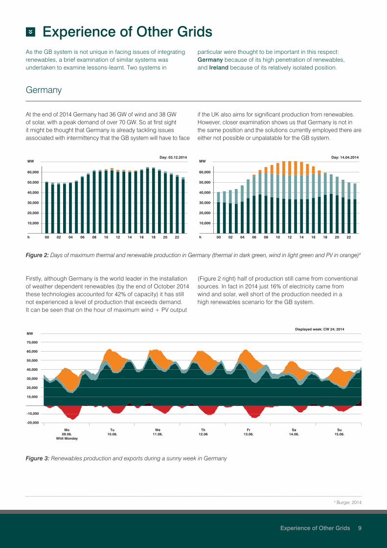
At the end of 2014 Germany had 36 GW of wind and 38 GW of solar, with a peak demand of over 70 GW. So at first sight it might be thought that Germany is already tackling issues associated with intermittency that the GB system will have to face
if the UK also aims for significant production from renewables. However, closer examination shows us that Germany is not in the same position and the solutions currently employed there are either not possible or unpalatable for the GB system.
Germany
Figure 3: Renewables production and exports during a sunny week in Germany
Figure 2: Days of maximum thermal and renewable production in Germany (thermal in dark green, wind in light green and PV in orange)4
Day: 14.04.2014
60,000
50,000
40,000
30,000
20,000
10,000
00 02 04 06 08 10 12 14 16 18 20 22h
MWDay: 03.12.2014
60,000
50,000
40,000
30,000
20,000
10,000
00 02 04 06 08 10 12 14 16 18 20 22h
MW
Displayed week: CW 24; 2014
70,000
60,000
50,000
40,000
30,000
20,000
10,000
Mo09.06.
Whit Monday
Tu10.06.
We11.06.
Th12.06
Fr13.06.
Sa14.06.
Su15.06.
MW
-10,000
-20,000
Firstly, although Germany is the world leader in the installation of weather dependent renewables (by the end of October 2014 these technologies accounted for 42% of capacity) it has still not experienced a level of production that exceeds demand. It can be seen that on the hour of maximum wind + PV output
(Figure 2 right) half of production still came from conventional sources. In fact in 2014 just 16% of electricity came from wind and solar, well short of the production needed in a high renewables scenario for the GB system.
4 Burger, 2014

10 Experience of Other Grids
Secondly, although renewables output in Germany is less than half of demand for nearly all of the time, much of the renewables production (typically half) is exported to its neighbours rather than displacing the highly emitting lignite plant. Figure 3 illustrates this well. Note how exports (red) are highly correlated with PV (orange) + wind (light green). Exports regularly peak around midday throughout the summer in concert with PV output, and it can be seen from above that they are particularly high on Monday (a public holiday) and Friday (a relatively windy day). It is unlikely that this could continue if Germany’s neighbours were to adopt a similar renewables strategy and also sought to export surplus production.
Thirdly, an examination of the output of fossil plant during these periods of high renewables output reveals that although gas and hard coal plant reduce load, nearly all the lignite plant continues to run baseload. The combination of its extremely high carbon intensity and poor flexibility makes lignite a poor choice as the requisite firm capacity. The continued use of GB’s coal fleet in this way would undermine any attempt to decarbonise and would be unacceptable in the long term.
Finally, Germany does not have its own isolated electricity system but has 60 circuits of 220kV and above connecting it to 9 surrounding countries. It is therefore very much part of a strongly interconnected European system that is 8 times its size. There is a huge benefit of being embedded in a large system – a large inertia is guaranteed and reserve and response services are shared so proportionally less is needed. Furthermore the peaks in wind and solar output tend to be smoothed by the larger geographic coverage.
Therefore Germany does not provide much evidence on how the GB system could deal with high penetration of renewables, as:
• Its production from wind and PV is still quite low compared to scenarios explored here
• Although well short of having surplus renewables generation it chooses to export a lot of production so that high carbon plant runs baseload
• Most of its immediate trading partners (with the exception of the small Danish system) have not yet constructed large amounts of wind and PV
• Germany benefits from being a small part of a very large synchronous system
Unlike Germany the electricity system of Ireland and Northern Ireland is a small synchronous system with modest DC links to the GB system. Its planned renewable generation is dominated by wind, with the aim of 5-6 GW of installed capacity by 2020, against a peak demand of around 7 GW. Currently just under 3 GW are connected so the system is perhaps facing similar issues to the ones that will face the GB system when it gets to 25 GW of Wind + PV.
To manage this EireGrid and SONI, the system operators, ensure that total generation from non-synchronous generation (which is mostly wind) never exceeds 50% of demand. This is achieved by curtailing wind output if this limit is about to be breached. There are plans to increase this to 75% as experience of managing the system grows.
The Annual Wind Constraint and Curtailment Report 20135 indicates that 3.2% of wind was curtailed over the year to stay within those limits. The wind capacity during this period was 2.2-2.6 GW providing about 16% of demand.
It is unlikely that the GB system would want to adopt this early curtailment as a means of dealing with intermittency issues and this is not seen as a long term solution by the Irish system operators. Although curtailment can alleviate immediate stability or grid constraint issues, in the longer term significant levels of curtailment increase the system cost of renewables and set an artificial barrier to their penetration. Therefore the modelling which follows allows renewables to generate as much as the demand allows, subject to the other constraints.
Ireland
5 EirGrid and SONI, 2014
Modelling 11
»
ModellingA new model, BERIC, was written by ERP to Balance Energy, Reserve, Inertia and Capacity requirements. The input data, its solution methodology and assumptions are described below.
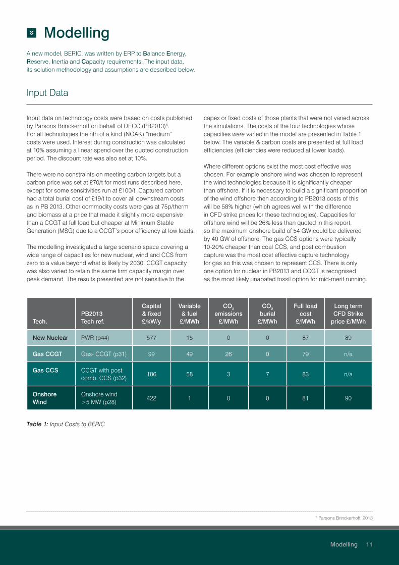
Input data on technology costs were based on costs published by Parsons Brinckerhoff on behalf of DECC (PB2013)6. For all technologies the nth of a kind (NOAK) “medium” costs were used. Interest during construction was calculated at 10% assuming a linear spend over the quoted construction period. The discount rate was also set at 10%.
There were no constraints on meeting carbon targets but a carbon price was set at £70/t for most runs described here, except for some sensitivities run at £100/t. Captured carbon had a total burial cost of £19/t to cover all downstream costs as in PB 2013. Other commodity costs were gas at 75p/therm and biomass at a price that made it slightly more expensive than a CCGT at full load but cheaper at Minimum Stable Generation (MSG) due to a CCGT’s poor efficiency at low loads.
The modelling investigated a large scenario space covering a wide range of capacities for new nuclear, wind and CCS from zero to a value beyond what is likely by 2030. CCGT capacity was also varied to retain the same firm capacity margin over peak demand. The results presented are not sensitive to the
capex or fixed costs of those plants that were not varied across the simulations. The costs of the four technologies whose capacities were varied in the model are presented in Table 1 below. The variable & carbon costs are presented at full load efficiencies (efficiencies were reduced at lower loads).
Where different options exist the most cost effective was chosen. For example onshore wind was chosen to represent the wind technologies because it is significantly cheaper than offshore. If it is necessary to build a significant proportion of the wind offshore then according to PB2013 costs of this will be 58% higher (which agrees well with the difference in CFD strike prices for these technologies). Capacities for offshore wind will be 26% less than quoted in this report, so the maximum onshore build of 54 GW could be delivered by 40 GW of offshore. The gas CCS options were typically 10-20% cheaper than coal CCS, and post combustion capture was the most cost effective capture technology for gas so this was chosen to represent CCS. There is only one option for nuclear in PB2013 and CCGT is recognised as the most likely unabated fossil option for mid-merit running.
Input Data
6 Parsons Brinckerhoff, 2013
Tech.PB2013 Tech ref.
Capital & fixed£/kW/y
Variable & fuel
£/MWh
CO2 emissions
£/MWh
CO2 burial
£/MWh
Full load cost
£/MWh
Long term CFD Strike
price £/MWh
New Nuclear PWR (p44) 577 15 0 0 87 89
Gas CCGT Gas- CCGT (p31) 99 49 26 0 79 n/a
Gas CCS CCGT with post comb. CCS (p32)
186 58 3 7 83 n/a
Onshore Wind
Onshore wind >5 MW (p28)
422 1 0 0 81 90
Table 1: Input Costs to BERIC

12 Modelling
If all of the costs have to be recovered through the selling of energy (e.g. through a CFD) then the price needed for nuclear is £87/MWh, which compares very favourably with the nth of a kind strike price of £89/MWh. For onshore wind a price of £81/MWh is needed, slightly less than the long term CFD strike price of £90/MWh. This gives confidence that the costs are consistent with the current market.
The availability of most plant types was a fixed value applicable across all scheduling points, but wind and PV availability followed time-varying profiles. The availability profile for wind was based upon the generation reported to Elexon during 20127. A check was made that this was a typical year by examining the profiles for the last five years. The profiles for 2012/13/14 were very similar in shape, but 2011 was significantly more ‘peaky’ and 2010 appeared to be have significantly lower load factors, confirming that 2012 was a good choice. The generation was converted to a load factor using the capacities reported to Energy Trends8 on a quarterly basis. Monthly variations in capacity were inferred from the rate of change of capacity between quarters.
This load profile was then scaled to meet the annual load factor which was set to 27.4%, a typical value for onshore wind. Given that the UK is likely to have a significant component of offshore wind the installed capacity of wind required to meet carbon targets is overstated, but costs will be understated than for a mixed portfolio.
PV availability was simulated using a curve rising from zero at sunrise to maximum at noon back to zero at sunset. This was randomly scaled by a factor between zero and 1 to represent the daily variability of insolation, and scaled again to give the expected profile for monthly energies as predicted by the EU/JRC online tool9 for Birmingham.
Demand data was based on 2012 outturns corrected for the small proportion of wind which is embedded and assumed to generate in line with the majority of the portfolio. This calculated consumer demand was then scaled to match the peak energy demand for 2030, derived from the National Grid’s Slow Progression scenario10, which gave an annual energy demand of 317 TWh.
7 Elexon, 20148 DECC, 20159 JRC web tool10 National Grid, 2013
Model runs were set up by taking data from the Slow Progression scenario, but each run is an ensemble of scenarios with varying amounts of new nuclear, onshore wind and gas-CCS capacity on the system. Any shortfall in firm capacity was made up with unabated CCGT so that de-rated capacity margin was always 10%. The capacities of the three exogenously variable technologies were allowed to vary widely, nuclear from 0-40 GW, wind from 0-56 GW and gas-CCS from 0-30 GW, covering the range of all likely outcomes by 2030. Figure 4 illustrates this alongside the fixed capacities taken from Slow Progression. In terms of capacity the most significant fixed technologies were 6 GW of biomass, 5 GW of PV and 4 GW of CHP. Biomass was modelled as having the same flexibility characteristics as coal plant. Pump storage was represented as 3 GW of highly flexible generation, but its pumping demand was neglected.
At the heart of BERIC is a linear programming (LP) solver, whose objective function is to minimise short run costs at each scheduling point in the scenario run. Points are scheduled independently from each other. The model is constrained to stay within the following bounds:
Methodology
Cap
acity
in M
od
el (
GW
)
120
100
80
60
40
20
0
CCGT
Gas CCS
Onshore Wind
New Nuclear
Slack
Sensitivityvariables
Fixed(SP 2030)
Old NuclearCHP − smallOilSolar PVBiomassHydroPumped StorageMarineNew NuclearOnshore WindCCS GasGas
Figure 4: Capacities of Technologies in the Model

Modelling 13
Mode DescriptionEnergy Provided Reserve Provided
Inertia added to sys. Short run cost
Off Offline 0 0 (except wind can provide 70% of curtailed energy)
0 0
MSG Running at minimum stable generation
MSG x Availability
(FL-SRL) x Availability
Full inertia Based on NFVOC*, fuel, carbon & efficiency at MSG
SRL Running at Spinning Reserve Level, the minimum load at which all of headroom can be provided as reserve
SRL x Availability
(FL-SRL) x Availability
Full inertia Based on NFVOC, fuel, carbon & efficiency interpolated between MSG & FL.
Full Load
Running at capacity rating Capacity x Availability
0 Full inertia Based on NFVOC, fuel, carbon & efficiency at FL
Table 2: Plant states in BERIC *Non Fuel Variable Operating Cost
1. Energy demand must be balanced exactly by generation. Demand is given by the 2012 shape scaled to meet 2030 Slow Progression peak energy demand (which is not that different to today’s demand).
2. There must be sufficient reserve to meet the requirement at all times. BERIC schedules against a reserve demand that represents the requirements for frequency response + faster reserve products covering timescales of seconds and minutes, but not hours. It is assumed that the system operator will need to cover the new larger maximum load loss designed to cover new nuclear and operating an array of generation on one double circuit. Wind and PV generation creates a demand for reserve cover at a rate of 17% of output, in line with typical values used by National Grid today.
3. There must be sufficient inertia to meet the requirement at all times. It is assumed that inertia levels will be allowed to drop from the current minimum level of 150 GW.s down to 90 GW.s following recent changes to the grid code. This improved the tolerance of the system to the Rate Of Change Of Frequency (ROCOF – see section on Inertia on page 25).
Generation is scheduled in fleets according to type, so the fleet of CCGTs is scheduled as one, all wind turbines as another etc. However the solver has freedom to assign any proportion of the fleet to one of four operating states. In effect then there are no quanta associated with individual units. As the proportions have to sum to 1 within a fleet, there are three independent variables per fleet. The four states are given in the Table 2 below.
In all modes fleets incur their long run costs of capex repayments and fixed opex.
• All markets are assumed to be free and fair. There is no modelling of policy costs (such as the effect of the mechanisms within the current trading arrangements or Electricity Market Reform) with the one exception of there being an exogenous cost to emit carbon
• New sources of flexibility from storage and demand side management were not modelled in BERIC, but the model never lacked sources of low carbon reserve and later calculations looked at their potential impact
• Existing storage (3 GW) was modelled as generation that was out of merit for bulk generation but cheap for the provision of inertial or reserve services. The demand of this storage was not included
• Interconnection was not modelled, so neither the provision of services nor the demand for services that might arise from overseas counterparties were included
• 2030 is modelled “stand alone” and not as a step on the way to 2050
• Only the effect on total system cost and emissions was considered and not wider benefits or implications of low carbon technologies reducing imports of fossil fuels or improving long term fuel security
Assumptions

14 Results
»
Results
The scenario underpinning the CCC’s 4th Carbon Budget had a decarbonisation of the grid down to 50 g/kWh. The November 2013 review11 confirmed that this level of decarbonisation by 2030 is on the most cost effective pathway to the 2050 target. DECC uses a central scenario that has a 2030 emissions intensity of 100 g/kWh. These two levels are illustrated in the results to demonstrate the likely range of outcomes.
Figure 5 shows how the carbon intensity varies with addition of wind to the base scenario, with differing levels of nuclear capacity. For the lower penetration levels the carbon free wind generation displaces emissions from gas plant and intensity falls, however, its effectiveness at abatement declines as more is added. Examination of the schedule shows that as wind is added it is displacing progressively lower carbon plant eventually causing significant levels of curtailment of its own output or that of other zero carbon plant.
Meeting Emission Targets with Nuclear and Wind
0
50
100
150
200
250
0 10 20 30 40 50 60
300
Wind capacity (GW)
Sys
tem
CO
2 In
tens
ity (
g/k
Wh
)
11 GWWind today
28 GWNREAP
133 g/kWh
CCC targetof 50 g/kWh
No new nuclear
+20 GW nuclear
Figure 5: Emissions as a function of wind and nuclear capacity
The top line represents a grid where wind is the only significant low carbon technology. In this set of mixed nuclear-wind scenarios it can be seen that even with the addition of 56 GW of onshore wind (5 x current levels and double the UK’s National Renewable Energy Action Plan (NREAP) for meeting EU targets) the grid intensity will only fall to around 180 g/kWh if there is no new nuclear capacity. The model though neglects the effect that new storage, demand side management or strong interconnection might have. Examination of the chart will help bound this benefit though if the initial slope of the upper curve (where displacement of fossil is completely effective) is taken to continue without diminishing as wind is added. This tangent represents the addition of an infinite amount of storage with no turnaround losses (or infinitely flexible demand/ interconnection). It can be seen that even with this benefit the emission intensity will only get to 133 g/kWh
even with 60 GW of onshore wind. This is because even if all of the 145 TWh of wind generation were usable, the remaining 172 TWh is mostly being met by fossil generation.
The series of lower lines represents the addition of 5 GW increments of nuclear capacity. The effectiveness of this is clear, showing that 20-25 GW of nuclear alongside the NREAP target for wind (or 30 GW of nuclear alone) will achieve the CCC’s 50 g/kWh decarbonisation target. Although this set of scenarios explored differing levels of nuclear, similar results would be obtained with any Zero Carbon Firm (ZCF) capacity so long as it emits no CO2 and provides capacity that is (on a fleet basis) as reliable as fossil plant. This could for example be CCS plant that burns sufficient biomass to offset the residual emissions or an unabated plant that burns biomass with no attributable emissions.
11 CCC, 2013
0510152025303540
0
10
20
30
50 g/kWh
Nuclear
CCS
Win
d
60
50
40
30
20
10
0
100 g/kWh
C c
d
bB
A
D
a
15
25
5
510152025303540
0
10
20
30
15
25
5
0
NREAP level
25 50 75
100
60
50
40
30
20
10
0
CCS
Win
d
Nuclear
Results 15
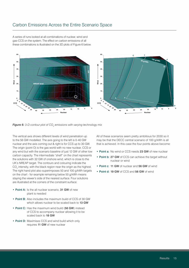
A series of runs looked at all combinations of nuclear, wind and gas-CCS on the system. The effect on carbon emissions of all these combinations is illustrated on the 3D plots of Figure 6 below.
Carbon Emissions Across the Entire Scenario Space
Figure 6: 3-D contour plot of CO2 emissions with varying technology mix
The vertical axis shows different levels of wind penetration up to the 56 GW modelled. The axis going to the left is 0-40 GW nuclear and the axis coming out & right is for CCS up to 30 GW. The origin (point O) is the gas world with no new nuclear, CCS or any wind but with the scenario baseline of just 12 GW of other low carbon capacity. The intermediate “shelf” on the chart represents the solutions with 32 GW of onshore wind, which is close to the UK’s NREAP target. The contours and colouring indicate the CO2 intensity, with the black region near the origin as the highest. The right hand plot also superimposes 50 and 100 g/kWh targets on the chart - for example remaining below 50 g/kWh means staying the viewer’s side of the nearest surface. Four solutions are illustrated at the corners of the constraint surface:
• Point A: Is the all nuclear scenario, 31 GW of new plant is needed
• Point B: Also includes the maximum build of CCS of 30 GW which allows nuclear to be scaled back to 13 GW
• Point C: Has the maximum wind build (56 GW) instead of CCS to accompany nuclear allowing it to be scaled back to 18 GW
• Point D: Maximises CCS and wind build which only requires 11 GW of new nuclear
All of these scenarios seem pretty ambitious for 2030 so it may be that the DECC central scenario of 100 g/kWh is all that is achieved. In this case the four points above become:
• Point a: No wind or CCS needs 23 GW of new nuclear
• Point b: 27 GW of CCS can achieve the target without nuclear or wind
• Point c: 11 GW of nuclear and 56 GW of wind
• Point d: 19 GW of CCS and 56 GW of wind

16 Results
It is worth highlighting the role of biomass at this point. All scenarios had 6 GW of biomass (mostly converted coal plant) and an examination of the schedules showed that its energy output was generally quite low. However alongside pump storage it provided a significant amount of the required reserve and response services by running at low load in times of greatest need, thus allowing flexibility services to be fulfilled with no additional emissions.
Examining a central scenario with 15 GW each of nuclear and CCS, and 24 GW of wind showed that biomass plant was providing 51% of the reserve and pump storage 34%.
A sensitivity analysis around this scenario was undertaken to see the effect of providing the reserve from elsewhere. If biomass was prevented from providing reserve, and nuclear and CCS were pretty inflexible (providing just 5% and 10% of their capacity as reserve respectively) then emissions increased markedly from 15 to 23 Mt as the model called upon unabated gas for this service. However if either nuclear or CCS were made flexible (40% reserve provision) then emissions returned to the 15-16 Mt level even without the biomass. This demonstrated the importance of a low carbon source of reserve, which could come from low carbon firm capacity or from sources not modelled such as new storage or demand side management.
Low Carbon Reserve Provision
To check these modelling conclusions, and to examine the effects behind them, some simplified merit order calculations were performed. The supply side was simplified to just three types of plant, namely:
• weather dependent renewables (an aggregate of PV, onshore and offshore wind that minimised curtailment),
• Zero Carbon Firm (ZCF), and
• unabated gas (representing a 25:75 mix of peaking and high efficiency plant).
For each half hour these were stacked, in that merit order, to meet demand. Three scenarios were constructed: one that was renewables only, one that was ZCF only and one that was an equal mix of renewables and ZCF in terms of energy available. Gas emissions were assumed to be 412 g/kWh but the messages that come out are not very sensitive to this. This should illustrate the main effects, although it should be remembered that in reality the system requirements for reserve and response provision will mean that curtailment and “diminishing returns” effects will occur at lower penetrations of zero carbon plant.
To illustrate these effects the results examined will start with low levels of penetration of just 20% of energy from zero carbon sources. Increasing low carbon capacities by a factor of four, in an attempt to meet 80% decarbonisation, demonstrates how curtailment can affect the ability to reach lower levels of grid carbon intensity. Finally the ability of storage and other time-shifting technologies to alleviate these issues is demonstrated with even higher levels of low carbon penetration.
The results are illustrated below in the traditional manner of a load duration curve based on 2012 data. The solid line represents demand throughout the year sorted such that peak demand is on the left and minimum demand on the right. The light green area represents the energy delivered by variable renewables, orange is from ZCF with the dark green representing unabated gas. The lower curve below the light green section represents the curve re-sorted by demand not met by variable renewable output; windless winter peak periods will still be on the left but the right-hand side becomes increasingly dominated by high renewable output periods as their penetration increases.
Checking BERIC with Merit Order Calculations

Results 17
70,000
60,000
50,000
40,000
30,000
20,000
10,000
Renewable Mix Zero Carbon Firm
Figure 7: The effect of 20% penetration of low carbon technologies on the load duration curve
The three plots in Figure 7 illustrate a relatively low level of penetration (17 GW each of PV and wind on the left, 8 GW of ZCF on the right). In each plot the sum of the orange and light green areas are equal, showing the delivery of 20% of
energy requirements in each scenario. The dark green area is the residual gas generation resulting in emissions of 330 g/kWh in all three scenarios.
70,000
60,000
50,000
40,000
30,000
20,000
10,000
Renewable Mix Zero Carbon Firm
Figure 8: High penetration levels of low carbon technologies showing spill
The second set of three plots in Figure 8 illustrates the quadrupling of the low carbon capacities from the 20% penetration scenario illustrated in Figure 7. Note now that curtailment of excess zero carbon generation is shown as the light orange area above the demand line. Clearly it can be seen to be worse in the renewables scenario than the ZCF scenario. In fact 11% of zero carbon production is curtailed in the former, 4% for the mixed scenario and 2% for the ZCF world. This illustrates how the diminishing returns
of adding variable renewables is more severe than adding ZCF - as wind and PV capacity is added most energy is now delivered at the right hand side of curve in the curtailment zone. However the challenge is to decarbonise the remaining dark green triangle on the left whilst minimising expenditure. The differing levels of curtailments mean that emissions in the three scenarios are quite different, from 128 g/kWh in the renewables scenario through 98 g/kWh for the mixed case to 91 g/kWh in the ZCF case.

18 Results
The calculations in the previous section have taken no account of the benefit of storage, demand side response or interconnectors to effectively reshape the demand curve to minimise curtailment. In reality an effective energy market may incentivise a range of these technologies and solutions if price differentials were sufficient to overcome costs. To explore this a storage algorithm was added to the half hour stacking calculation to illustrate its benefits. If there was over-generation the store would fill until it reaches maximum, and then empty, at an efficiency of 75%, over the subsequent daily peak period
whenever that would displace gas. A storage capacity of 30 GW was added, representing a ten-fold increase on GB’s current pump storage capacity but a larger storage volume was examined from 6 hour’s generation (similar to today’s storage that cycles on a daily basis) to 48 hours. This was applied to the high renewables scenario (i.e. where there was sufficient variable renewables to supply 80% of demand). A third test was performed to see if expanding the variable renewables to theoretically cover 100% of demand would eliminate fossil.
The Value of Storage in Solving Curtailment Issues
70,000
60,000
50,000
40,000
30,000
20,000
10,000
6h storage, 80% renew 48h storage, 80% renew 48h storage, 100% renew
Figure 9: Showing effect of storage in utilising excess zero carbon generation
Figure 9 above shows the results. The dark red area illustrates the curtailed energy that now goes into storage, and storage generation displaces gas as represented by the pale red area. With the 30 GW of 6h storage then nearly half the curtailed energy is utilised and the generation reduces emissions by 16 g/kWh to 112 g/kWh. Increasing the storage volume to cover 48 hours of generation improves the effectiveness of the storage significantly, emissions fall to 98 g/kWh and curtailed
energy falls to just 1% of total energy demand. Pushing the variable renewables build so its potential output matches demand in the final chart shows that although the storage is well used there is still a significant spill (8% of generation) and fossil is required to fill 12% of demand. This scenario just meets the 50g/kWh target, the remaining emissions coming from a “stubborn triangle” at the bottom left of the load duration curve that is difficult to reach.
7.9 TWh 6.5 TWh
Fossil
Net weekly balance
Curtailment
Results 19
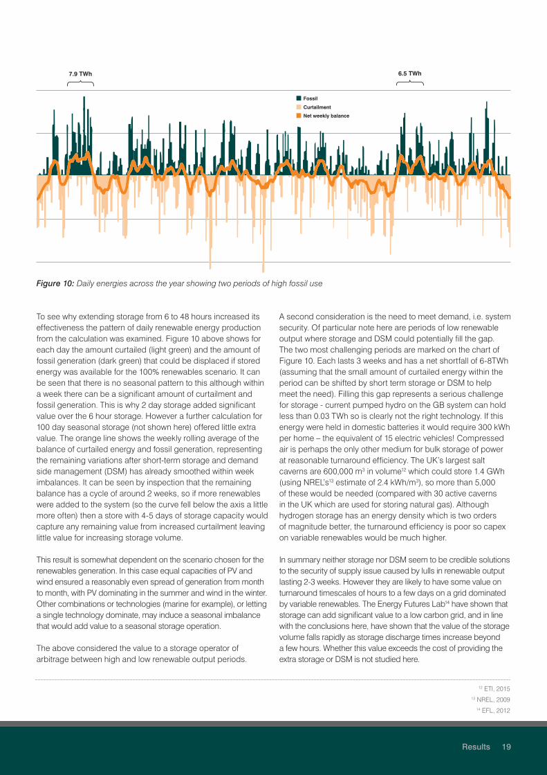
Figure 10: Daily energies across the year showing two periods of high fossil use
To see why extending storage from 6 to 48 hours increased its effectiveness the pattern of daily renewable energy production from the calculation was examined. Figure 10 above shows for each day the amount curtailed (light green) and the amount of fossil generation (dark green) that could be displaced if stored energy was available for the 100% renewables scenario. It can be seen that there is no seasonal pattern to this although within a week there can be a significant amount of curtailment and fossil generation. This is why 2 day storage added significant value over the 6 hour storage. However a further calculation for 100 day seasonal storage (not shown here) offered little extra value. The orange line shows the weekly rolling average of the balance of curtailed energy and fossil generation, representing the remaining variations after short-term storage and demand side management (DSM) has already smoothed within week imbalances. It can be seen by inspection that the remaining balance has a cycle of around 2 weeks, so if more renewables were added to the system (so the curve fell below the axis a little more often) then a store with 4-5 days of storage capacity would capture any remaining value from increased curtailment leaving little value for increasing storage volume.
This result is somewhat dependent on the scenario chosen for the renewables generation. In this case equal capacities of PV and wind ensured a reasonably even spread of generation from month to month, with PV dominating in the summer and wind in the winter. Other combinations or technologies (marine for example), or letting a single technology dominate, may induce a seasonal imbalance that would add value to a seasonal storage operation.
The above considered the value to a storage operator of arbitrage between high and low renewable output periods.
A second consideration is the need to meet demand, i.e. system security. Of particular note here are periods of low renewable output where storage and DSM could potentially fill the gap. The two most challenging periods are marked on the chart of Figure 10. Each lasts 3 weeks and has a net shortfall of 6-8TWh (assuming that the small amount of curtailed energy within the period can be shifted by short term storage or DSM to help meet the need). Filling this gap represents a serious challenge for storage - current pumped hydro on the GB system can hold less than 0.03 TWh so is clearly not the right technology. If this energy were held in domestic batteries it would require 300 kWh per home – the equivalent of 15 electric vehicles! Compressed air is perhaps the only other medium for bulk storage of power at reasonable turnaround efficiency. The UK’s largest salt caverns are 600,000 m3 in volume12 which could store 1.4 GWh (using NREL’s13 estimate of 2.4 kWh/m3), so more than 5,000 of these would be needed (compared with 30 active caverns in the UK which are used for storing natural gas). Although hydrogen storage has an energy density which is two orders of magnitude better, the turnaround efficiency is poor so capex on variable renewables would be much higher.
In summary neither storage nor DSM seem to be credible solutions to the security of supply issue caused by lulls in renewable output lasting 2-3 weeks. However they are likely to have some value on turnaround timescales of hours to a few days on a grid dominated by variable renewables. The Energy Futures Lab14 have shown that storage can add significant value to a low carbon grid, and in line with the conclusions here, have shown that the value of the storage volume falls rapidly as storage discharge times increase beyond a few hours. Whether this value exceeds the cost of providing the extra storage or DSM is not studied here.
12 ETI, 201513 NREL, 2009
14 EFL, 2012

20 Results
Interconnectors could benefit the GB system by connecting it to markets with different weather influences and so take excess generation at times of GB surplus and return carbon free generation at times of low renewable output. However these interconnected markets would not always be in the right state to do this – for instance when similar weather was being experienced in the neighbouring markets that had installed similar renewable energy technologies. So in effect they would act like storage with an availability that was significantly lower than a physical asset.
The only exception might be for an interconnection to a market such as NordPool that has significant reservoir hydro. In this case, if NordPool ran its hydro plant for the benefit of the GB system the interconnector would look like a storage system with good turnaround efficiencies. According to Rondeel15 most of NordPool’s hydro is located in Norway which has ~28 GW (used mostly for its domestic needs). About 17 GW
of this is controllable reservoir with a total storage capacity of 84 TWh. A further 5-7 GW could be built without too large of an environmental impact. In theory then 20+ GW of the UK’s storage needs could come from Norway, and the 8 TWh needed to fill the low wind gaps could probably be accommodated. In practice though, the UK may find other EU nations also wanting to use NordPool’s balancing capabilities and some, unlike the UK, are already connected. Alternatively, interconnection could be used to allow storage to be managed at a European level; significant reductions in the volume of storage needed could be achieved if energy was only stored when there was no scope for reducing the output of fossil plant anywhere in Europe.
It is likely then that interconnection can help, especially to NordPool, but is unlikely to provide a complete solution as other markets compete for the same resources. Furthermore, interconnection does not usually come cheap and a careful examination of the costs involved would be necessary.
Interconnectors
15 Rondeel, 2012
In relation to reducing curtailment DSM in its simplest form is the delaying or advancing of demand by a period to a time of surplus renewables. However most DSM discussed in the literature is for within-day changes to the demand (e.g. delayed washing, controlling EV charging ready for the morning, turning off aircon and recovering shortly afterwards). In this mode of operation it looks like storage with a few hours capacity and a very high efficiency, but with various restrictions and constraints associated with the needs of
the devices in question. In terms of effect on the whole market it is therefore unlikely to be more effective than the 6 hour storage modelled above, but could prove to be significantly less costly to implement.
The 8 TWh gap is not going to be solved through DSM as it represents an average reduction of 15 GW for 3 weeks. There is little domestic activity that can be delayed that long and the reduction needed exceeds average industrial demand.
Demand Side Management

Results 21
Table 3 summarises the curtailment issues and the solutions to enable carbon targets to be approached. Percentage values are all in terms of annual energy demand.
Summary of Load Duration Calculations
Capacities (GW) Results
Scenario Wind PV ZCF StorageRE Avail (%dem)
ZCF avail (%dem)
ZC spill (%dem)
Gas gen (%dem)
CO2
(g/kWh)
RE.20 17 17 - - 20% - - 80% 330
Mix.20 8 8 4 - 10% 10% - 80% 330
ZCF.20 - - 8 - - 20% - 80% 330
RE.80 68 68 - - 80% - 11% 31% 128
Mix.80 34 34 16 - 40% 40% 4% 24% 98
ZCF.80 - - 32 - - 80% 2% 22% 91
RE.80 + 6h store
68 68 - 30 80% - 6% 27% 112
RE.80 + 48h store
68 68 - 30 80% - 1% 24% 98
RE.100 + 48h store
85 85 - 30 100% - 8% 12% 50
ZCF.90 + 24h store
- - 36 6 - 90% 1% 12% 50
Table 3: Effect of plant mix on CO2 Emissions
The CO2 values in orange demonstrate achieving an emission level of less than 100 g/kWh, with two scenarios at the end designed to achieve the CCC target of 50 g/kWh. However the scale of engineering to achieve even this by 2030 should not be underestimated. The ZCF.90 scenario which achieved the 50 g/kWh represents either 25-30 new nuclear reactors, 36 GW of CCS transporting and sequestering more than 100 Mt of CO2 p.a., or the burning of 150 Mt of biomass p.a. It also doubles GB storage output capacity and quadruples storage volume. The RE.100 scenario represents 20-30,000 wind turbines with a 4 kW PV panel per household, and alongside that a vast increase in storage volume by a factor of 50, equivalent to 60 cables to Norway, or a 50 kWh battery in every household.
Given the scale of these investments it seems that a mix of technologies are going to be required. The scenario with 170 GW of variable renewables is particularly unrealistic by 2030, and even longer term it is questionable whether the scale of DSM, interconnection and storage required just to reach 50 g/kWh with variable renewables alone is achievable or desirable. With the diminishing returns of adding more variable renewables, and the need to cover 2-3 week periods of low renewable output, a complete decarbonisation is going to need a significant amount of firm low carbon capacity.
22 Results
This section returns to BERIC to compare the costs of delivering a low carbon system with various combinations of nuclear, wind and gas-CCS. The total system cost here is a summation of all the costs associated with the generation fleet. This includes the capital costs, the fixed costs and operating costs such as fuel, emissions and CO2 disposal. As described in the assumptions there is no cost or income associated with any other policy measures, most of which move money around within the modelled system.
The system cost results are of course very sensitive to the inputs on fuel costs and technology capex, and so the absolute costs presented here are only applicable to this particular scenario based on the PB 2013 inputs as described in the section on input data. However the messages about how the relative value of technologies change with different grid mixes are generally applicable.
Effect on Total System Cost
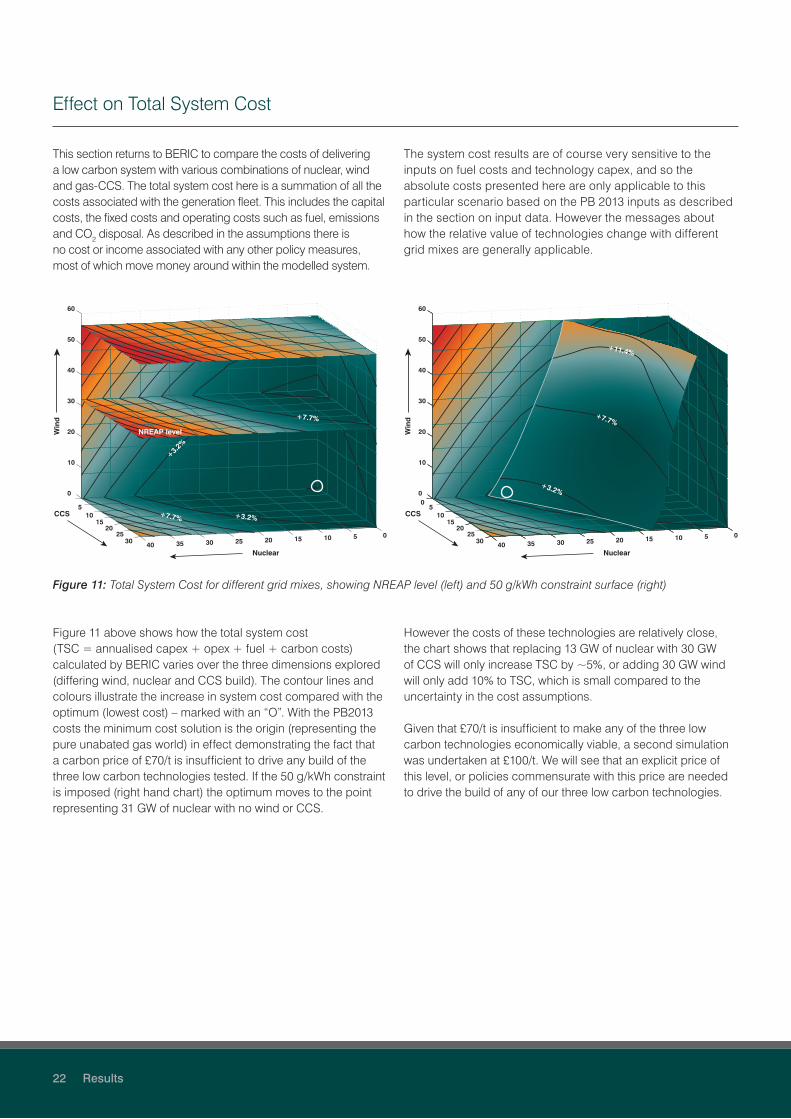
Figure 11: Total System Cost for different grid mixes, showing NREAP level (left) and 50 g/kWh constraint surface (right)
Figure 11 above shows how the total system cost (TSC = annualised capex + opex + fuel + carbon costs) calculated by BERIC varies over the three dimensions explored (differing wind, nuclear and CCS build). The contour lines and colours illustrate the increase in system cost compared with the optimum (lowest cost) – marked with an “O”. With the PB2013 costs the minimum cost solution is the origin (representing the pure unabated gas world) in effect demonstrating the fact that a carbon price of £70/t is insufficient to drive any build of the three low carbon technologies tested. If the 50 g/kWh constraint is imposed (right hand chart) the optimum moves to the point representing 31 GW of nuclear with no wind or CCS.
However the costs of these technologies are relatively close, the chart shows that replacing 13 GW of nuclear with 30 GW of CCS will only increase TSC by ~5%, or adding 30 GW wind will only add 10% to TSC, which is small compared to the uncertainty in the cost assumptions.
Given that £70/t is insufficient to make any of the three low carbon technologies economically viable, a second simulation was undertaken at £100/t. We will see that an explicit price of this level, or policies commensurate with this price are needed to drive the build of any of our three low carbon technologies.
NREAP level
+7.7% +3.2%
60
50
40
30
20
10
0
CCS
Win
d
Nuclear
15
25
5
+3.2%
+7.7%
0510152025303540
10
20
300510152025303540
0
10
20
30
Nuclear
CCS
Win
d
60
50
40
30
20
10
0
15
25
5
+11.4%
+7.7%
+3.2%
Results 23
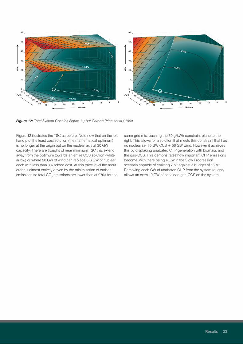
Figure 12: Total System Cost (as Figure 11) but Carbon Price set at £100/t
Figure 12 illustrates the TSC as before. Note now that on the left hand plot the least cost solution (the mathematical optimum) is no longer at the origin but on the nuclear axis at 30 GW capacity. There are troughs of near minimum TSC that extend away from the optimum towards an entire CCS solution (white arrow) or where 20 GW of wind can replace 5-6 GW of nuclear each with less than 3% added cost. At this price level the merit order is almost entirely driven by the minimisation of carbon emissions so total CO2 emissions are lower than at £70/t for the
same grid mix, pushing the 50 g/kWh constraint plane to the right. This allows for a solution that meets this constraint that has no nuclear i.e. 30 GW CCS + 56 GW wind. However it achieves this by displacing unabated CHP generation with biomass and the gas-CCS. This demonstrates how important CHP emissions become, with there being 4 GW in the Slow Progression scenario capable of emitting 7 Mt against a budget of 16 Mt. Removing each GW of unabated CHP from the system roughly allows an extra 10 GW of baseload gas-CCS on the system.
+7.4% +3.7%
60
50
40
30
20
10
0
CCS
Win
d
Nuclear
15
25
5
+7.4%
0510152025303540
10
20
30
+7.
4%
+7.4%
+14.8%+11.1%
0+3.7%
0510152025303540
0
10
20
30
Nuclear
CCS
Win
d
60
50
40
30
20
10
0
15
25
5
+3.7%
+7.4%
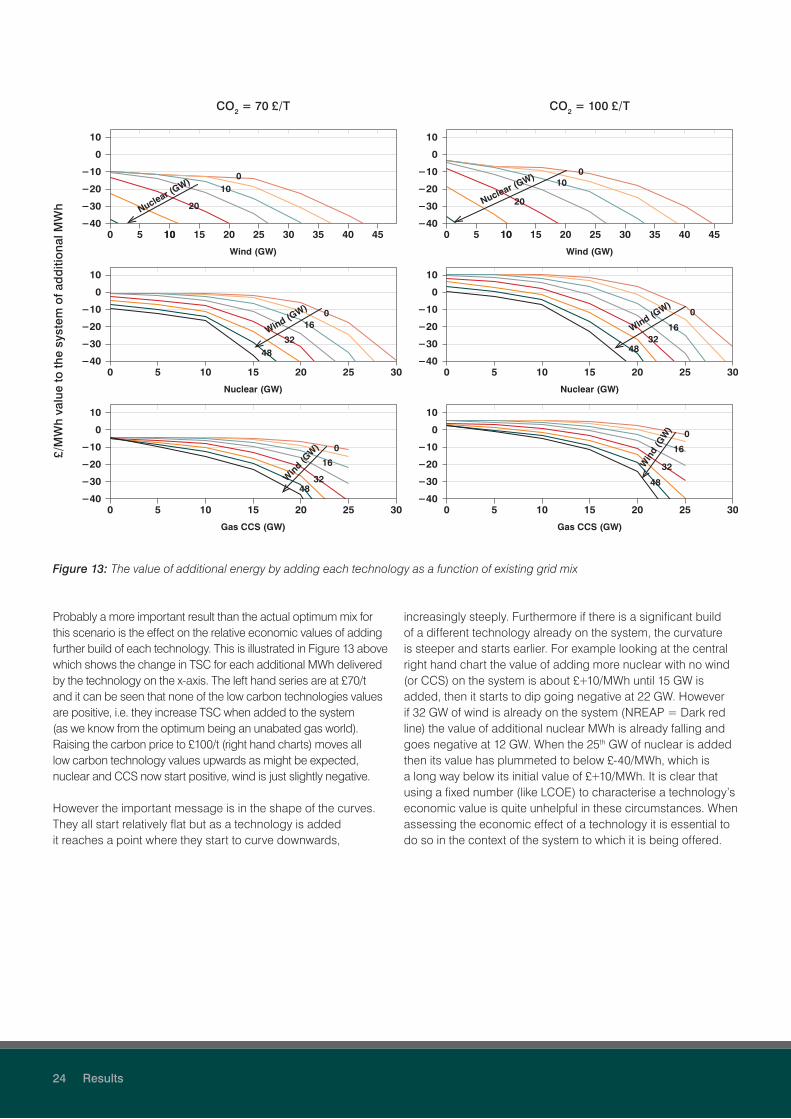
Figure 13: The value of additional energy by adding each technology as a function of existing grid mix
−40
−30
−20
−10
0
10
0 5 10 15 20 25 30
Gas CCS (GW)
0
16
32Win
d (G
W)
48
−40
−30
−20
−10
0
10
0 5 10 15 20 25 30
Nuclear (GW)
016
32Wind (G
W)
48
−40
−30
−20
−10
0
10
0 5 1010 15 20 25 30 35 40 45
Wind (GW)
010
20Nuclear (GW)
−40
−30
−20
−10
0
10
0 5 10 15 20 25 30
Gas CCS (GW)
0
16
32Win
d (G
W)
48
−40
−30
−20
−10
0
10
0 5 10 15 20 25 30
Nuclear (GW)
0
1632
Wind (GW)
48
−40
−30
−20
−10
0
10
0 5 1010 15 20 25 30 35 40 45
Wind (GW)
010
20Nuclear (GW)
CO2 = 70 £/T CO2 = 100 £/T
£/M
Wh
valu
e to
the
syst
em o
f ad
diti
ona
l MW
h
Probably a more important result than the actual optimum mix for this scenario is the effect on the relative economic values of adding further build of each technology. This is illustrated in Figure 13 above which shows the change in TSC for each additional MWh delivered by the technology on the x-axis. The left hand series are at £70/t and it can be seen that none of the low carbon technologies values are positive, i.e. they increase TSC when added to the system (as we know from the optimum being an unabated gas world). Raising the carbon price to £100/t (right hand charts) moves all low carbon technology values upwards as might be expected, nuclear and CCS now start positive, wind is just slightly negative.
However the important message is in the shape of the curves. They all start relatively flat but as a technology is added it reaches a point where they start to curve downwards,
increasingly steeply. Furthermore if there is a significant build of a different technology already on the system, the curvature is steeper and starts earlier. For example looking at the central right hand chart the value of adding more nuclear with no wind (or CCS) on the system is about £+10/MWh until 15 GW is added, then it starts to dip going negative at 22 GW. However if 32 GW of wind is already on the system (NREAP = Dark red line) the value of additional nuclear MWh is already falling and goes negative at 12 GW. When the 25th GW of nuclear is added then its value has plummeted to below £-40/MWh, which is a long way below its initial value of £+10/MWh. It is clear that using a fixed number (like LCOE) to characterise a technology’s economic value is quite unhelpful in these circumstances. When assessing the economic effect of a technology it is essential to do so in the context of the system to which it is being offered.
24 Results
Results 25
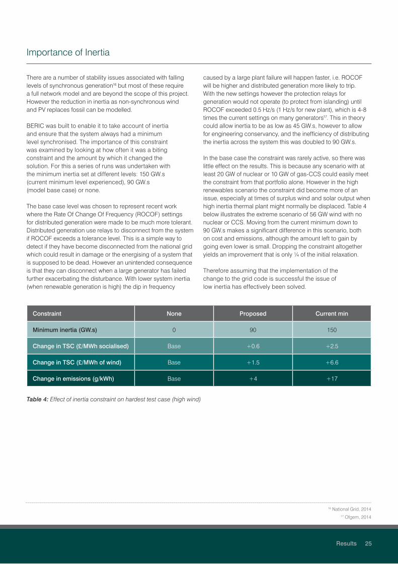
There are a number of stability issues associated with falling levels of synchronous generation16 but most of these require a full network model and are beyond the scope of this project. However the reduction in inertia as non-synchronous wind and PV replaces fossil can be modelled.
BERIC was built to enable it to take account of inertia and ensure that the system always had a minimum level synchronised. The importance of this constraint was examined by looking at how often it was a biting constraint and the amount by which it changed the solution. For this a series of runs was undertaken with the minimum inertia set at different levels: 150 GW.s (current minimum level experienced), 90 GW.s (model base case) or none.
The base case level was chosen to represent recent work where the Rate Of Change Of Frequency (ROCOF) settings for distributed generation were made to be much more tolerant. Distributed generation use relays to disconnect from the system if ROCOF exceeds a tolerance level. This is a simple way to detect if they have become disconnected from the national grid which could result in damage or the energising of a system that is supposed to be dead. However an unintended consequence is that they can disconnect when a large generator has failed further exacerbating the disturbance. With lower system inertia (when renewable generation is high) the dip in frequency
caused by a large plant failure will happen faster, i.e. ROCOF will be higher and distributed generation more likely to trip. With the new settings however the protection relays for generation would not operate (to protect from islanding) until ROCOF exceeded 0.5 Hz/s (1 Hz/s for new plant), which is 4-8 times the current settings on many generators17. This in theory could allow inertia to be as low as 45 GW.s, however to allow for engineering conservancy, and the inefficiency of distributing the inertia across the system this was doubled to 90 GW.s.
In the base case the constraint was rarely active, so there was little effect on the results. This is because any scenario with at least 20 GW of nuclear or 10 GW of gas-CCS could easily meet the constraint from that portfolio alone. However in the high renewables scenario the constraint did become more of an issue, especially at times of surplus wind and solar output when high inertia thermal plant might normally be displaced. Table 4 below illustrates the extreme scenario of 56 GW wind with no nuclear or CCS. Moving from the current minimum down to 90 GW.s makes a significant difference in this scenario, both on cost and emissions, although the amount left to gain by going even lower is small. Dropping the constraint altogether yields an improvement that is only ¼ of the initial relaxation.
Therefore assuming that the implementation of the change to the grid code is successful the issue of low inertia has effectively been solved.
Importance of Inertia
16 National Grid, 201417 Ofgem, 2014
Constraint None Proposed Current min
Minimum inertia (GW.s) 0 90 150
Change in TSC (£/MWh socialised) Base +0.6 +2.5
Change in TSC (£/MWh of wind) Base +1.5 +6.6
Change in emissions (g/kWh) Base +4 +17
Table 4: Effect of inertia constraint on hardest test case (high wind)

To assess the importance of modelling reserve and response a run was done where the requirement for these was set to zero and comparing with one with a very high level (30% of renewable generation). The effect of including reserve and response constraints is to increase total system cost. The additional socialised cost varied with grid mix from 0.5 to 4.4 £/MWh, the biggest effect was seen in the high wind, high CCS, low nuclear scenarios.
The effect of this on emissions though was complex and strongly dependent on the grid mix. Modelling reserve in
some cases increased emissions by up to 39 g/kWh, in other cases it reduced them by 12 g/kWh. This latter, perhaps unexpected result, occurred in a high fossil/moderate wind world where adding the reserve requirement shifted generation from unabated gas to biomass.
The message here is clear, taking proper account of reserve and response is likely to make a significant difference to the important parameters in a scenario such as cost and in particular CO2 emissions.
The Importance of Reserve and Response
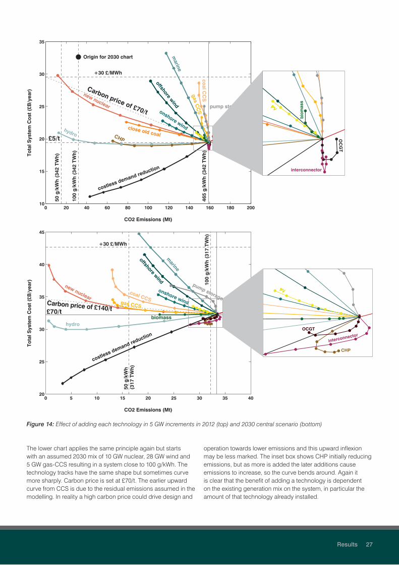
The results presented so far have focussed on three main technologies for decarbonisation, namely nuclear, wind and gas-CCS. However there were 17 technology tranches modelled within BERIC so a brief comparison was made of the effect of changing the capacity each technology by means of the following two diagrams. The curves emanating out of a central scenario show the change in emissions (x-axis) and Total System Cost (y-axis) of adding another increment of that technology, usually 5 GW. The upper chart of Figure 14 has the 2012 system as a starting point with carbon priced at £5/t. Most technologies fall in the top left quadrant, which results in abatement at a cost. As a low carbon technology is added, new nuclear for example, emissions are reduced (line steps to the left) but eventually emission reductions become smaller and the line curves upwards as abatement become costly. This is usually as a result of curtailment increasingly limiting the output whilst capex costs remain the same. Hydro and CHP appear
to be relatively cheap, the first additions actually saving money and carbon. Closing old coal also reduces emissions albeit at a cost to the system. CCS technologies are shown as high cost and ineffective at reducing emissions, this is entirely a result of the low carbon price in 2012 which was insufficient for them to perform any more than a peaking duty.
In the top right are actions that increase cost and emissions, so ought to be avoided. Closing old nuclear fits into this category, suggesting that life extension should be sought where safe. In the bottom left there is only one curve. This shows increments of 10% reductions in demand. The line assumes that this comes at zero cost. In reality this is probably not the case so actual curves for demand reduction will lie above this curve. Also illustrated are two carbon price lines, for example the one at £70/t delimits technologies that are economic at this price (below the line) from those that aren’t (above the line).
Comparison of all Technology Options
26 Results
Results 27
Figure 14: Effect of adding each technology in 5 GW increments in 2012 (top) and 2030 central scenario (bottom)
The lower chart applies the same principle again but starts with an assumed 2030 mix of 10 GW nuclear, 28 GW wind and 5 GW gas-CCS resulting in a system close to 100 g/kWh. The technology tracks have the same shape but sometimes curve more sharply. Carbon price is set at £70/t. The earlier upward curve from CCS is due to the residual emissions assumed in the modelling. In reality a high carbon price could drive design and
operation towards lower emissions and this upward inflexion may be less marked. The inset box shows CHP initially reducing emissions, but as more is added the later additions cause emissions to increase, so the curve bends around. Again it is clear that the benefit of adding a technology is dependent on the existing generation mix on the system, in particular the amount of that technology already installed.
0 5 10 15 20 25 30 35 4020
25
30
35
40
45
CO2 Emissions (Mt)
Tota
l Sys
tem
Co
st (
£B/y
ear) 10
0 g
/kW
h (
317
TWh
)
50 g
/kW
h
(317
TW
h)
costless demand reduction
+30 £/MWh
£70/t
hydro
new nuclear
close old
nuclear
coal CCS
marine
offshore wind
onshore wind
pump storagegas CCSCarbon price of £140/t
biomass
OCGT
interconnector
CHP
PVPV
0 20 40 60 80 100 120 140 160 180 20010
15
20
25
30
35
CO2 Emissions (Mt)
Tota
l Sys
tem
Co
st (
£B/y
ear)
50 g
/kW
h (
342
TWh
)
100
g/k
Wh
(34
2 TW
h)
costless demand reduction
Origin for 2030 chart
+30 £/MWh
£5/t
465
g/k
Wh
(34
2 TW
h)
hydro
new nuclear
CHP
close old coal close old nuclear
coal C
CS
marine
offshore wind
onshore wind
pump storage
gas CC
S
Carbon price of £70/tPVPVPV
bio
mas
s
OC
GT
interconnector

»
Key Observations Hitting 50 g/kWh drives the need to meet the vast majority
of residual demand (after allowing for variable renewable generation) in a low carbon manner. Even acknowledging the possible contribution of DSM, interconnectors and storage to firming up weather dependent renewables, a deep decarbonisation of the grid will need a significant penetration of zero carbon firm capacity. In ERP’s modelling a minimum of 13 GW of new zero carbon firm capacity was required to meet 50 g/kWh. Given the long timescales for introducing these technologies there is a pressing need to prioritise their introduction if carbon reduction targets are to be met.
Of the issues examined it is rare for lack of inertia to be a biting constraint, the recent changes to disconnection settings for distributed generation will allow the system to tolerate lower values of inertia than at present. However modelling the requirements for frequency response and fast reserve make a significant difference to total system cost and especially to emissions, and so cannot be ignored. The need for frequency response is driven by issues other than the technology mix, and so is relatively easy to model, but the need for fast reserve and STOR are most critical and dependent on technology choice.
Using DECC’s cost estimates18 the differences in economic value to the system between the key options examined (nuclear, gas-CCS and onshore wind) are much smaller than the margin of error estimating those costs. Therefore it’s difficult to claim any one of these is the optimal solution to progress grid decarbonisation. Furthermore the value to the system is highly dependent on the technology mix on the system, and the effect of diminishing returns reduces the value of all technologies as they are added, but especially so of variable renewables which generate an increasing proportion at times of surplus energy.
Technologies like DSM/flexibly operated interconnectors and new storage will help optimise the system, especially one with a high penetration of PV and wind, but will probably not bring fundamental changes to the ultimate solution. In helping to reduce curtailment from a good balance of wind and PV there appears to be little value to extending storage capacities beyond a few days.
Germany’s Energiewende does not provide a good example for the GB system which is unable to rely on being embedded within a much larger system. Germany’s current model phasing out much of its zero carbon firm capacity in favour of high carbon inflexible lignite also runs directly against all the recommendations here.
The implication of valuing firm capacity and ancillary services is that it would be helpful to consider changing the retail market pricing structure to reflect the actual costs.
18 Parsons Brinckerhoff, 2013
28 Key Observations

Conclusions 29
»
ConclusionsThe Need for Zero Carbon Firm Capacity
A zero- or very low- carbon system with weather dependent renewables needs companion low carbon technologies to provide firm capacity
The modelling indicates that the 2030 decarbonisation targets of 50 or even 100 g/kWh cannot be hit by relying solely on weather dependent technologies like wind and PV alone. Simple merit
order calculations have backed this up and demonstrated why this is the case, even with very significant storage, demand side measures or interconnection in support. There is a need to have a significant amount of zero carbon firm capacity on the system too - to supply dark, windless periods without too much reliance on unabated fossil. This firm capacity could be supplied by a number of technologies such as nuclear, biomass or fossil CCS.
The Need for Market Pull for Ancillary Services
Policy makers and system operators need to value services that ensure grid stability so new providers feel a market pull
Currently some necessary services (e.g. inertia/ frequency response) are provided free or as a mandatory service. However, traditional providers of these services (fossil plant)
are closing or becoming uneconomic to run, and at the same time, demand is growing (especially for fast reserve and response). Weather dependent renewables are not consistent suppliers of these services but new providers can’t develop in the absence of a market signal.
The Need for a Holistic Approach to Valuing Technologies
A holistic approach to system cost would better recognise the importance of firm low carbon technologies and the cost of balancing the system
The modelling has demonstrated that the value to the system of a technology is dependent on the existing generation mix and the services which that technology can provide. The former means that a technology cannot be characterised by a single number such as levelised cost of energy (LCOE). Firstly because energy is only one of
a number of essential services that technologies provide to (or require from) the grid; and secondly because the existing grid mix has a very substantial influence on the value of the services provided by additional technology.
Whilst this report has focused on generation technologies, it is important to recognise that demand reduction through energy efficiency will have a role to play in reducing carbon emissions and must be considered alongside low carbon generation technologies.

30 Recommendations
»
Recommendations A much deeper examination of the issues raised here
is needed. This modelling and analysis has only just begun to scratch the surface and the ERP does not have the resource or capabilities to take this work much further. It is therefore encouraging to see a number of studies and model upgrades being commissioned (by DECC and CCC) and proposed (by Imperial College via SuperGen) as this report is being published.
A significant amount of new zero carbon firm capacity is essential to decarbonisation but leading technologies such as nuclear and CCS require long lead times. Therefore meeting emission targets for 2030 requires action today if these technologies are to be part of the solution.
One of the key conclusions is that providers of ancillary services need to feel a market pull. Therefore it is recommended that policy makers in DECC and experts in National Grid consider how new providers can be given the financial comfort needed to underpin their development and deployment before traditional providers disappear.
The European Commission’s Smart Grid Task Force have recently published an analysis of the regulations surrounding demand side flexibility and recommendations for policy makers and grid operators19. Although these are focussed on just distributed sources of flexibility from consumers this is one important new source for ancillary services. Furthermore, many of the recommendations could be taken more generically to help the development of other sources. So where the explanatory text mentions consumers and aggregators it could be broadened to include new generation, interconnectors and storage too. ERP advises that the following recommendations from the Smart Grids Task Force20 should be examined by policy makers and National Grid for applicability across all providers to the GB system.
• No. 2: Equal Access to Electricity Markets for all providers
• No. 3: Contractual arrangements should be simple, transparent and fair
• No. 4: Standardised measurement of flexibility
• No. 12: Incentivise grid operators to enable and use flexibility, investing for meeting 2030 targets rather than focus on short-term optimisation
• No. 13: Improving price signals for providers
19 Smart Grids Task Force, 201520 Smart Grids Task Force, 2015

References 31
»
ReferencesBurger, B., 2014. Fraunhofer Institute for Solar Energy Systems ISE, Electricity production from solar and wind in Germany in 2014, December 29, 2014
CCC, 2013. Fourth Carbon Budget Review - part 2, The cost-effective path to the 2050 target, December 2013
DECC, 2015. Energy Trends, https://www.gov.uk/government/collections/energy-trends, as updated on 26/3/2015
Dynamic Demand. http://www.dynamicdemand.co.uk/chart.htm
EirGrid and SONI, 2014. Annual Wind Constraint and Curtailment Report 2013
Energy Futures Lab, Strbac et al, 2012. Strategic Assessment of the Role and Value of Energy Storage Systems in the UK Low Carbon Energy Future. Report for the Carbon Trust
Energy Technologies Institute (ETI), 2015. Hydrogen - The role of hydrogen storage in a clean responsive power system
JRC. Tool for PV output: Photovoltaic Geographic Information System. Web tool, http://re.jrc.ec.europa.eu/pvgis/apps4/pvest.php
National Grid, 2013, UK Future Energy Scenarios – July 2013 edition
National Grid, 2014. System Operability Framework (SOF), September 2014
National Renewable Energy Laboratory (NREL), 2009. Lifecycle Cost Analysis of Hydrogen Versus Other Technologies for Electrical Energy Storage
Ofgem, 2010. Ref 133/10: 29/10/10. Proposal to modify the Security and Quality of Supply Standard by increasing the infeed loss risk limits (GSR007)
Ofgem, 2014. Decision: Changes to the Distribution Code and Engineering Recommendation G59: Frequency Changes during Large Disturbances and their Impact on the Total System
Parsons Brinckerhoff, 2013. Electricity Generation Cost Model – 2013 for DECC. 3512649A (non renewable) and 3511633B (renewable)
Rondeel, W.G.J., 2012. HIT Telemark University College. Hydro Electricity and Storage Capabilities in Norway – can they be useful for Europe? Frühjahrstagung des Arbeitskreises Energie in der Deutschen Physikalischen Gesellschaft Berlin, 26. bis 28. März 2012
Smart Grids Task Force, 2015. Expert Group 3, Regulatory Recommendations for the Deployment of Flexibility, January 2015

ENERGY RESEARCH PARTNERSHIP 11 PRINCES’ GARDENS, LONDON SW7 1NA www.erpuk.org