liow to simplify fluidflow calculationsSolving f/uid f/ow problems has a/waysbeen done by s/ow, inefficient trial anderror methods. Here is a way to solvethese prob/ems direct/y, in two steps

Paul Page Austin, Arthur G. MeKee & Co., San Mateo,Calif.

THE USUAL METHOD of solving a fluid flow problem,using rational formulas, is by the use of a chart showingthe relationship between the Reynolds number R and theFanning Coeffieient or frietion eoeffieient f in the wellknown Fanning equation:

f v2 Lh=--D2 gIn most fluid flow problems either the Aow rate or the

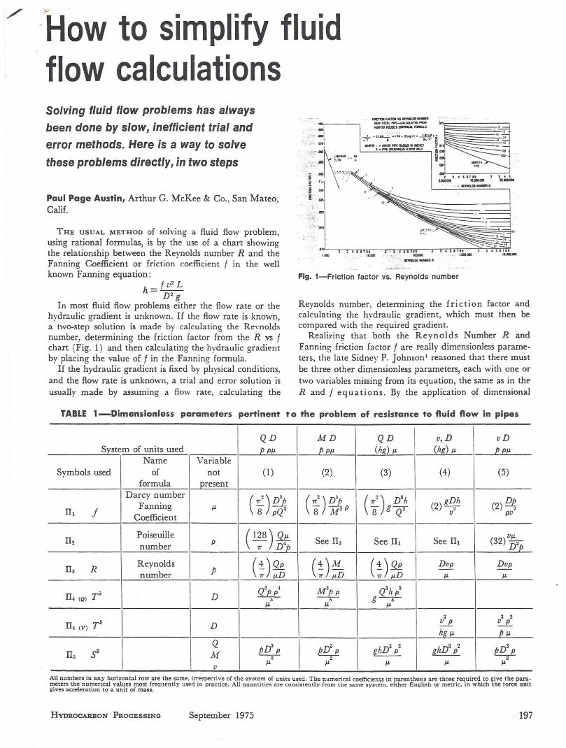
hydraulie gradient is unknown. If the flow rate is known,a two-step solution is made by ealeulating the Revnoldsnumber, determining the frietion faetor from the R vs fehart (Fig. 1) and then ealculating the hydraulic gradientby placing the value of f in the Fanning formula.

If the hydraulie gradient is fixed by physical eonditions,and the flow rate is unknown, a trial and errar solution isusually made by assuming a flow rate, ealculating the

Flg. 1-Friction factor vs. Reynolds number

Reynolds number, determining the friction faetor andealculating the hydraulic gradient, whieh must then becompared with the required gradient.

Realizing that both the Reynolds Number R andFanning friction faetor f are really dimensionless parame-ters, the late Sidney P. Johnson1 reasoned that there mustbe three other dimensionless pararneters, eaeh with one ortwo variables missing from its equation, the same as in theR and I e q u a t i o n s. By the applieation of dimensional

TABLE l-Dimensionless parameters pertinent to the problem of resistance to fluid flow in pipes

QD MD QD I u,D uD!System of units used f!. PIl f!. PIl (hg) Il

\

(hg) Il f!. PIlName Variable

Symbols used of not (I) (2) (3) I (4) (5)formula present

«') D'h IDarey number ( 7r2)~ (7r2 )~ (2) g~h (2)~Fanning IlIII j Coeffieient8 pQ2 8 M2P 8 g Q2 ; U pu

II2Poiseuille (t28) !Q:. See II3 See III See III (32)~number P 7r D4f!. D2f!.

II3 R Reynoldsp (±) Qp (~)~ (±) Qp Dup Dup

number 7r J.l.D 11" J.l.D J.I. J.I.

II4 (Q) 1'5 DQ3p p4 M3pp Q3h/

5 s s=:r:IJ. Il J.I.3 3 2

II4 (V) T5 D ~ ~hg Il I!.IJ.

QpD

3P pD

3P ghD3 p2 ghD3 p2 pD3 PIIó S2 M 2 2 2J.I. J.I. IJ. IJ. IJ.

uAli numbers in any horizontal row are the sarne. irrespective 01 the svstern 01 units used. The numerical coefficients in parenthesis are those required to give the para-rneters the numerical values most frequentlv used in practice. All quarrrit ies are consistently from lhe same evstem. either English or rnetric, in which the force unitgives acceleration to a unit of mass.

HYDROCARBONPROCESSING September 1975 197

HOW TO SIMPLIFY FLUID FLOW CALCULATIONS

analysisv" he derived the formulas for the three otherdirnensionless parameters.

Two of these parameters plotted versus t numbers, to-gether with the Reynolds number vs. f chart, makes itpossible to solve any flow problem directly, without trialand error.

ln 1883, Osborn Reynolds' published his paper in whichhe showed the difference between viscous or nonturbulentfiow and turbulent flow and gave his formula which deter-mined which of the two conditions existed in a pipe, forany set of given fíow conditions. Since then many papershave been published giving curves showing the relation-ship between the Reynolds number (R) and the frictionfactor f. These curves, alI obtained by experiment, werefor various sizes of pipe and were often difficult to corre-late over the entire range of pipe sizes. Some of them alsohad the fault that the lines continued to droop as theReynolds numbers became larger, whereas modern curvesof this kind flatten out to constant values of f =. highReynolds numbers. ln 1944, Lewis Moody' published hispaper in which he introduced a new variable, inside pipewalI roughness. This was done by plotting a series ofcurves showing the R vs. f relationship, each line for afixed ratio of roughness (expressed in thousands of aninch) divided by inside pipe radius in inches. These curvesflatten out to constant values of f at high Reynoldsnumbers.

Final1y in 1943, Hunter Rouse" published his paper inwhich he had derived an empirical formula containingthe four variables, R, f, r (pipe radius) and k (roughness).

This formula gives relationships between f and R whichreflect correct values from the lowest values of R in thebeginning of the turbulent region, out to the higher values,where f becomes constant. This is the set of curves inFig. 1. The roughness is that of new clean steel pipe,k = 0.0018 incho

The advantage of using the Hunter Rouse formula toproduce a set of R vs. f curves (with an assumed fixedvalue for k) is that the curves will always be practicallyidentical, irrespective of who ca1culates and plots them.

Using Buckingham's I1 designation, Table 1 shows thefive dimensionless parametric equations written in variousforms and the variable missing from each.

The first (I1l) and third (I1a) are the f and R parame-ters, respectively, and the other three are those derivedby Johnson.

Thus, it becomes evident that any two parameters canbe plotted against each other, but it is also clear that mostof the 10 charts that could thus be obtainable would be oflittle value.

In any chart of two parameters plotted against eachother, one must be an independent variable, and the otherthereby automatically becomes the dependent variable.For example, in the R vs. f chart, the Reynolds numberis the one that is always calculated and is thus the inde-pendent variable and f becomes the dependent variable,the value of which is required.

The parameter I1~ excludes density. As density does notinfluence the head loss in either turbulent or nonturbulentflow, and since density is never an unknown variable in afluid flow problem, no further consideration will be givento I12•

TABLE2-Rational flow formulas

F1uld Reynolds number Head or preseure lose

Liquide7742 Dv Aj~fR= h =

11

Q QS BjQ2sLR = C-- = C- P=DI' DIJ. D6

IValues of A Values of B

Q - Rate 01 Values 01 C Q ~ Rate offlow in flow in L in miles L in M leet L in miles L in M feet

gpm 3162 gpm 164.3 31.1 71.1 13.47

bph I 2213 bph 80.5 15.25 34.8 6.60

bpd 92.2 bpd 0.1398 0.0265 0.0605 0.0115I

Gaeea-BjZT~~2L*Volume p/ _ P

22Baele

CQG =

R = IJ.DP = Bj TGQ2L**

2P1D5

Values of BQ = Rate of fíow Values of C Q == Volume flow rate at standard conditions***

expressed in*** L in miles L in M leet

scfm 29.0 scfm 0.2767 0.0524

Mscfh 483.6 Mscfh 76.56 14.5

MMscf per 24 hrs. 20,150 MMscf per 24 hrs, 133.580 25,300

Wel~hM2Rate

AnyM Pt = 0.00336 j pD6

FluldR = 6.32 IJ.D

2

Valid for ali fluids P = 1.294 j V ~L ****For nomenclature-See Table 4

·See note I, Table 4 ·.See note 2. Table 4 • •• See note 3. Table 4 ·*·*See note 4. TabIe 4 tPressure drop per 1.000 ft.

198 September 1975 HYDROCARBON PROCESSING

With the above facts in mind, it now becomes apparent"that the only two additional charts really necessary tomake a direct solution of a fiow problem are the inde-pendent parameters Il, (with diameters unknown) andIló (with flow rate unknown) each plotted versus Il1 (I)as the dependent parameter.

Only occasionally is the unknown variable the pipediameter. In the smaller sizes, only commercial sizes areavailable so a very rough estimate will give the range ofsize within one, or at the most, two commercial sizes. Thisparameter will perhaps be most usefui for determininglarger sizes of pipe, where commercial sizes above 42inches are not available.

Throughout the entire range of turbulent flow, Il1 (I)varies only from 0.04 down to 0.006 in numerical value.Its use as the dependent parameter in ali problems ofturbulent How, therefore, besides being consistent withcurrent engineering practice, permits an accurate graph-ical presentation readable to three significant places if alidata to be displayed are less than two cycles of logrithmeticpaper. Therefore the use of III (I) as the dependentparameter in turbulent flow problems is the most con-venient, and it has been so plotted in Figs. 1, 2 and 3.These are necessary to maintain equality. Also g, theacceleration of gravity appears in some equations. Here itis a dimensionless constant, having the property of forceper unit of mass, which is necessary if h is regarded as aslope. If h is considered in the nature of energy loss perunit mass of fluid and length of pipe, which is equallypermissible, g becomes merely a co n s t a n t of propor-tionality.

There are several interesting singularities in Table 1where some of the Ils contain only three variables. Forexample III can be expressed in three variables, D, Q andh.•but this is no particular advantage, as III is never cal-culated as an independent parameter. The parameter Ila

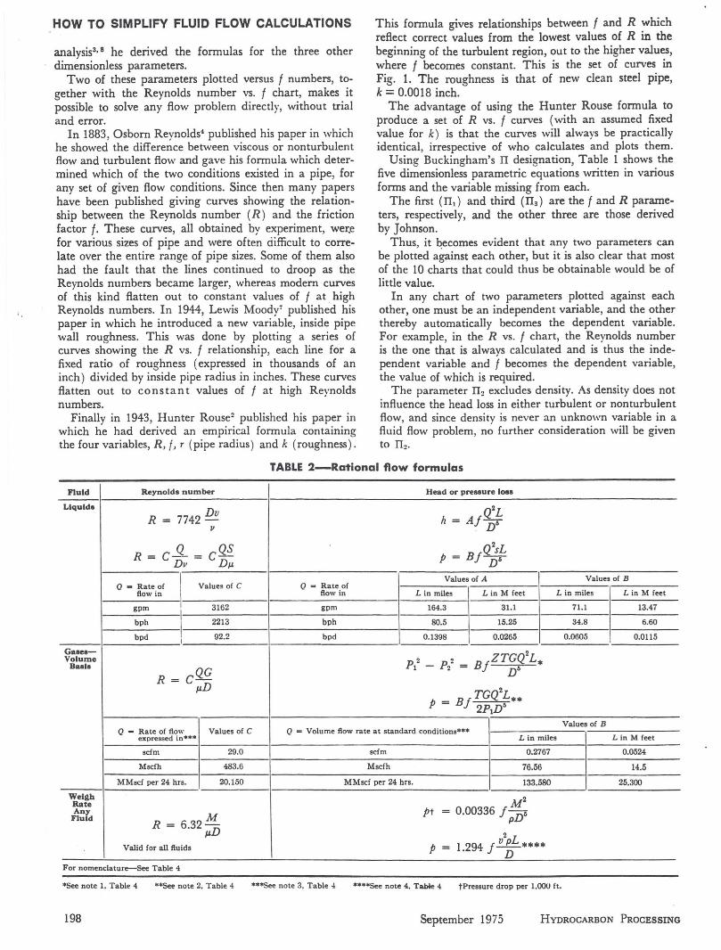
Fig. 2-Friction facto r VS. S number.

(R) can be expressed in terms of mass rate offiow, diame-ter and viscosity, without p.

This permits the general method of fiow calculation tobe applied to almost any case of gas flow, irrespective ofthe pressure drop. When any one value of Il is determinedon a curve, all the others become fixed. In the case ofgases f.J. is a function of temperature but substantially inde-pendent of pressure or density, and therefore IlJ is con-stant from one end of a line of uniform diameter to theother so long as the temperature in the line is fairly con-stant. All the Ils are constant if the expansion of gas as itfiows through a line is isothermal.

The scale of f has been made rather large so it can beeasily read to three significant figures. The horizontallength of 4 cycles has been compressed into about 1.5times the one cycle vertical scale. This makes for thesmooth line slope downward roughly 30 degrees and givesthe greatest accuracy of representation possible in a givenamount of chart space.

Figs. 2 and 3 do not show TI" and TI., respectively, directlyin the form given in Table 1, but instead show the square

TABLE3-Dimensionless parameter formulas with coefficients for use with commercial (engineering) units

Fluld Parameter

T number T = (Ilj/5 S number S= (Il,/12Liquida (Q3p 4) 1/5 (Q3 hs5) 1/5 (pD3)1/2 (hD3)1/2

T = F = N-- S = X IIS1/2 = y--IJ. IJ. 11

Values of F Va!ues of M Values of X Va!ues of YQ - Rate of

L in rniles L in M feetflow expressed in L in miles L in M feet L in H rniles L in M feet L in rniles L in M feet

gprn 10.1 14.1 8.58 12.0 2.65 6.09 1.74 4.01

bph 8.19 11.4 6.93 9.66

bpd 1.22 1.70 1.03 1.44

Gases[ ( P/

T-: :22) Q3G4J 1/5

S( p/ _ p/ yl2 D3/2Gl/2

T= = X TOL IJ.FIJ.

Values or F Va!ues of X

Q = Ra te of flow expressed in L in rniles L in M feet L in miles L in M feet

scfrn 0.282 0.394 0.390 0.895

MMscf per 24 hours 14.3 20.0

Vapors ( 3 ) 1/5 ( 3) 1/2Steam T = 0.149 0!J!pJ... S 0.771 P pD=IJ. IJ.

For nornenclature-See Tab!e 4

HYDROCARBON PROCESSING September 1975 199

OW TO SIMPLlFY FLUID FLOW CALCULATIONS

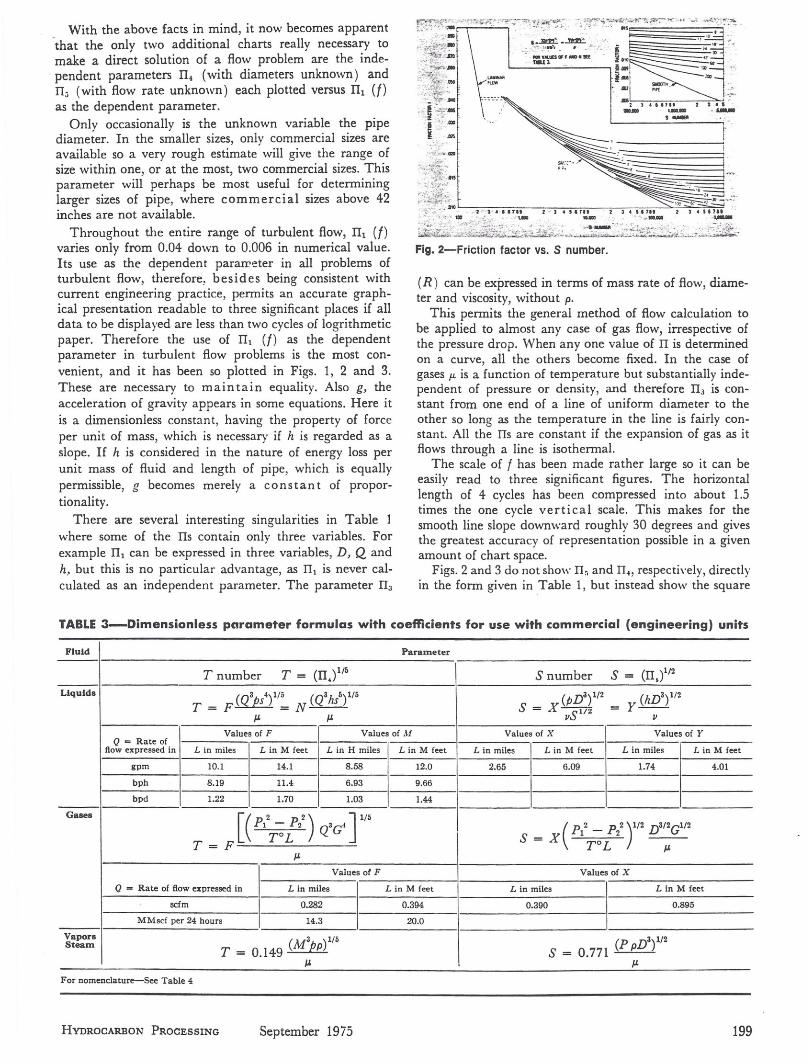
Fig. 3-Friction factor VS. T number.

root of lI, designated S and the fifth root of TI. designatedT. The reason for this alternation in the first place is togive S and T ab o u t the same magnitude as R, theReynolds number. The S number has roughly one-sevenththe value of R, while the T number has roughly two-fifthsthe value of R. In the second place, the numerical valuesof both values TI,. and IT. are uncomfortably large tohandle even with the notation of powers of 10. In particu-lar, the maximum value of IT I looks like a figure of astro-nomical magnitude. Fractional exponents introduced byusing S instead of TI" are no great objection, as thev can beread easily from a slide rule. Use of the fifth root of TI. isnot quite so easy to calculate on a slide rule, but actuallyT will not be used as often as S,

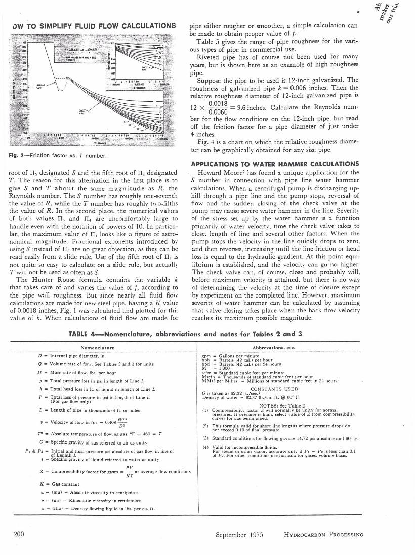
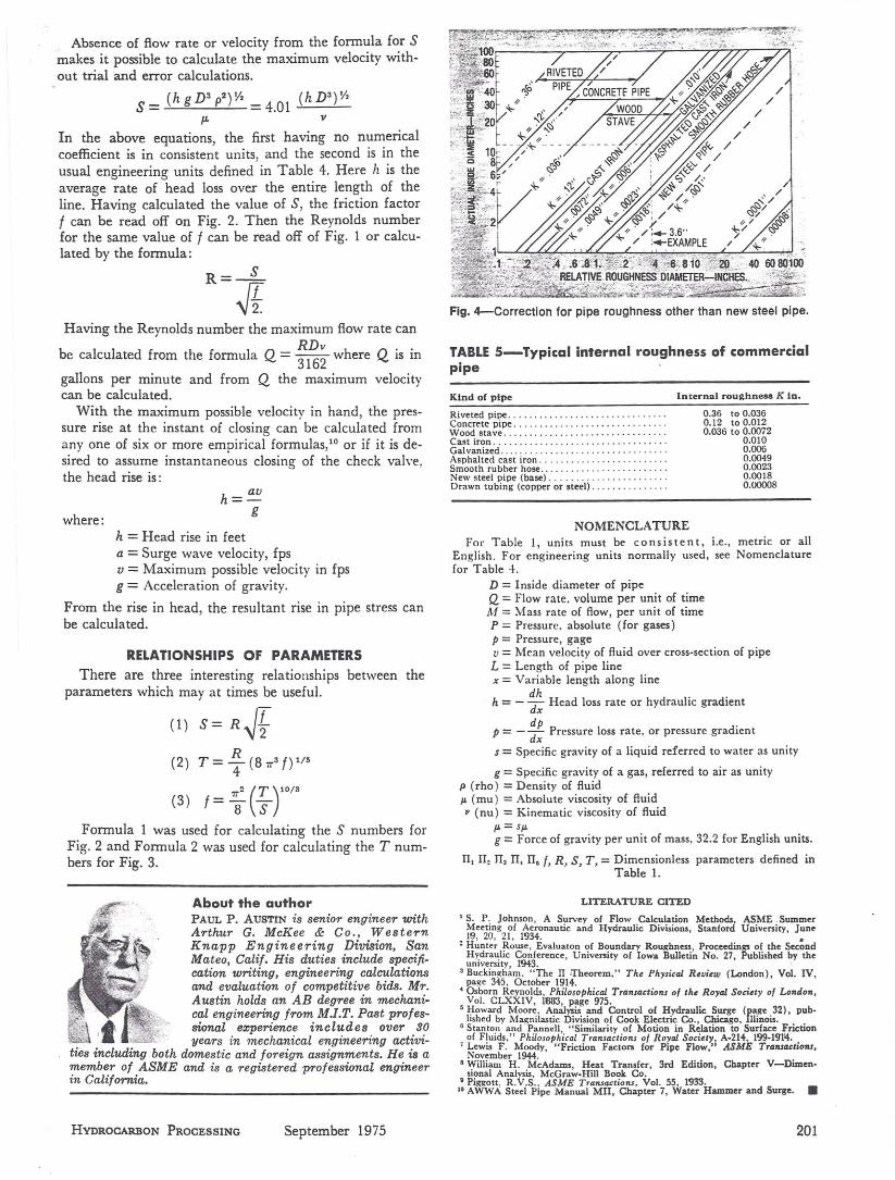
The Hunter Rouse formula contains the variable kthat takes care of and varies the value of f, according tothe pipe wall roughness. But since nearly ali fluid flowca!culations are made for new steel pipe, having a K valueof 0.0018 inches, Fig. 1 was calculated and plotted for thisvalue of k, When calculations of fiuid flow are made for

pipe either rougher or smoother, a simple ca!culation canbe made to obtain proper value of f·

Table 5 gives the range of pipe roughness for the vari-ous types of pipe in commercial use.

Riveted pipe has of course not been used for manyyears, but is shown here as ao example of high roughnesspIpe.

Suppose the pipe to be used is 12-inch galvanized. Theroughness of galvanized pipe k = 0.006 inches. Then therelative roughness diameter of 12-inch galvanized pipe is

12 X 0.0018 = 3.6 inches. Calculate the Reynolds num-0.0060

ber for the fiow conditions on the 12-inch pipe, but readoff the friction factor for a pipe diameter of just under4 inches.

Fig. + is a chart on which the relative roughness diame-ter can be graphically obtained for any size pipe.

APPLlCATIONS TO WATER HAMMER CALCULATIONSHoward Moere" has found a uniqueapplication for the

S number in connection with pipe line water harnmercalculations, When a centrifugal pump is discharging up-hill through a pipe line and the pump stops, reversal offlow and the sudden closing of the check valve at thepump may cause severe water hammer in the line. Severityof the stress set up by the water hammer is a functionprimarily of water velocity, time the check valve takes toelose. length of line and severa I other factors. When thepllmp stops the velocity in the line quickly drops to zero,and then reverses, increasing until the line friction or headloss is equal to the hydraulic gradient. At this point equi-librium is established, and the velocitv can go no higher.The check valve can, of course, elose and probably will,before maximum velocity is attained. but there is no wayof determining the velocitv at the time of closure exceptby experiment on the completed line. However, maximumseverity of water hammer can be ca!Culated by assumingthat valve elosing takes place when the back flow velocityreaches its maximurn possible magnitude.

Nomenclature

TABLE4-Nomenclature, abbreviations and notes for Tables 2 and 3

Abbrevations. etc.

D = Internal pipe dia meter. in.

Q = Volume rate of fiow. See Tables 2 anel 3 for units

.\1 =- Mass rale of fíow, lbs. per hour

p -= Total pressure 10505 in psi in lerigt h of Line L

h = Total head loss in it. of liquid in length of Line L

P = Total loss of pressure in psi in length of Line L(For gas flow only)

L = Length of pipe in thousands of it. or miles

gpm11 = Velocity of fiow in fps = 0.408-

D2

TO = Absolute temperature of flowing gas. °F + 460 = T

G = Specific gravity of gas referred to air as unity

P, & P2 = Initial and final pressure psi absolute of gas fiow in line ofof Length L

s = Specific gravitv of liquíd referred to water as unit v

PVZ = Compressibilitv factor for gases = - at average fiow conditions

KT

K = Gas constant

". = (mu) = Absolute viscositv in centipoises

\I = (nu) = Kinematic víscosit y in centistokes

p = (rho) = Densit y flowing Iiquid in lbs. per cu. ft.

gprn =- Gallons per minutebph = Barrels 142 ~al.) per hourbpd = Barrels (42 gal.) per 24 hoursM = 1.000scirn = Standard cubic feet per minuteMscf h = Thousands ai standard cubic feet per hourr...1~lsi per 24 hrs. = Millions or standard cubic ieet in 24 hours

CONST.-\:-.ITS USEDG is taken as 62.32 ft./sec.2Densit y of water = 62.37 lb./cu. ft. @ 60° F

NOTES: See Table 2O) Compressibility facto r Z wi ll normally be uni t y for normal

pressures, If pressure is hig h, select value of Z from cornpressibilit vcurves for zas bei ng pi ped ,

(2) This formula valid for short tine lengths where pressure drops donot exceed 0.10 of final pressure.

(3) Standard conditions for fiowing gas are 14.72 psi absolute and 60° F.

(4) Valid for incompressible fíuids.For steam or other vapor. accu ra te only if PI - P2 is less than 0.1of P2. For other conditions use formula for gases. volume basis.

200 September 1975 HVDROCARBON PROCESSING

Absence of flow rate or velocity from the formula for Smakes it possible to calculate the maximum velocity with-out trial and error calculations.

(hgD3p2)Y, (hD3)Y,S = = 4.01 "'-----'--p. v

In the above equations, the first having no numericalcoefficient is in consistent units, and the second is in theusual engineering units defined in Table 4. Here h is theaverage rate of head loss over the entire length of theline. Having calculated the value of S, the friction factorf can be read off on Fig. 2. Then the Reynolds numberfor the same value of f can be read off of Fig. 1 or calcu-lated by the formula:

Having the Reynolds number the maximum flow rate can

be calculated from the formula Q = :1~;where Q is in

gallons per minute and from Q the maximum velocitycan be calculated.

With the maximum possible velocity in hand, the pres-sure rise at the instant of closing can be calculated fromany one of six or more empirical Iorrnulas.!" or if it is de-sired to assume instantaneous closing of the check valve,the head rise is:

where:

h= avg

h = Head rise in feeta = Surge wave velocity, fpsv = Maximum possible velocity in fpsg = Acceleration of gravity.

From the rise in head, the resultant rise in pipe stress canbe calculated.

RELATIONSHIPS OF PARAMEnRSbetween theThere are three interesting relationships

parameters which may at times be useful.

(1) S= R~~

(2) T = .li. (8 7T3 f) 1/5

4

(3) _ 7T2 (T )10/3f-- -8 S

Formula 1 was used for calculating the S numbers forFig. 2 and Formula 2 was used for calculating the T num-bers for Fig. 3.

About the authorPAUL P. AUSTIN is senior engineer withArthur G. McKee & c«, Weste'/'nKnapp Engineering Division, SanMateo, Calif. His duties include specifi-cation writing, engineering calculationsand evaluation of competitive bids. Mr.Austin holds an AB deçree in mechani-cal engineering [rom M.I.T. Past projee-sional experience includes over 30

. yearsin mechanical engineering activi-ties including both domestic and foreign assignments. He is amember of ASME and is a registered professional engineerin California.

HYDROCARBON PROCESSING September 1975

Fig. 4-Correction for pipe roughness other than new steel pipe.

TABLE5-Typical interna I roughness of commercialpipe

Klnd o( pípe Internal rougbnese K Ia.

Riveted pipe .Concretc pipe .Wood 8tave ..........•............... · ·Cast íron .Gal vanized .Asphalted cast iron .Smooth rubher hose ' ............•New steel pipe (base) . . . . .Drawn tubing (copper or steel) .

0.36 to 0.0360.12 to 0.0120.036 to 0.0072omo

0.0060.00490.00230.00180.()()()()8

NOMENCLATUREFor Table I, units must be consistent, i.e., metric or all

English. For engineering units nonnally used, see Nomenclaturefor Table .J..

D = Inside diameter of pipeQ = Flow rate. volume per unit of timeM = Mass rate of flow, per unit of timeP = Pressure. absolute (for gases)p = Pressure, gagev = Mean velocity of fluid over cross-section of pipeL = Length of pipe linex = Variable length along line

h = - :~ Head 1055 rate or hydraulic gradient

dp 1 diP = -"'dx' Pressure oss rate, or pressure gra ient

S = Specific gravity of a liquid referred to water as unity

g = Specific gravity of a gas, referred to air as unityp (rho) = Density of fluidp. (mu) = Absolute viscosity of fluidv (nu) = Kinernatic viscosity of fluid

p. = s p:g = Force of gravity per unit of mass, 32.2 for English units.

n, rr, rr, rr, rr, I,R, S, T, = Dimensionless parameters defined inTable 1.

LlTERATURE ClTED

'S. P, Johnson, A Survey of Flow Calculation Methods, ASME .SummerMeeting of Aeronautic and Hvdraulic Divisions, Stanford University, June

_ 19, 20, 21, 1934. •• Hunter Rouse, Evaluaton of Boundary Roughness, Proceedings of the SecondHydraulic Conference, University of Iowa BulIetin No. 27, Published by theurnversrtv, 1943. I

3 Buckingham , "The TI Theorem." The Ptvysicai Review (London), Vol. IV,page 345, October 1914.

• Osborn Reynolds, Philosophicol Transaetions of lhe Royol Socie/y of London,Vol. CLXXIV, 1883, page 975.

'Howard Moore. Analvsis and Control of Hvdraulic Surge (page 32), pub-lished by Magnilastic Division oí Cook Electric Co., Chicago, lIlinoi s,

• Stanton and Pannell, "Similarity of Motion in Relation to Surface Frictionof Fluids," Phllosophical Transactions of Royal Soeiety, A·214. 199-191'l.

1 Lewis F. Moody, "Friction Factors for Pipe Flow," ASME Transaetlons,November 1944.

'William H. McAdams, Heat Transfer, 3rd Edition, Chapter V-Dimen·sional Analysis, McGraw·HilI Book Co.

• Piggott, R.V.S .• ASME Transactions, Vol. 55, l!ln.'o AWWA Steel Pipe Manual MIl, Chapter 7, Water Hammer and Surge. •

201