author query form - welcome to epic - epicepic.awi.de/30759/3/jasr_10886.pdfauthor query form...

Our reference: JASR 10886 P-authorquery-v10

AUTHOR QUERY FORM

Journal: JASR

Article Number: 10886

Please e-mail or fax your responses and any corrections to:

E-mail: [email protected]

Fax: +31 2048 52799

Dear Author,

Please check your proof carefully and mark all corrections at the appropriate place in the proof (e.g., by using on-screen annotation in the PDF file) orcompile them in a separate list. Note: if you opt to annotate the file with software other than Adobe Reader then please also highlight the appropriate placein the PDF file. To ensure fast publication of your paper please return your corrections within 48 hours.

For correction or revision of any artwork, please consult http://www.elsevier.com/artworkinstructions.

Any queries or remarks that have arisen during the processing of your manuscript are listed below and highlighted by flags in the proof. Click on the ‘Q’

link to go to the location in the proof.

Location in

article

Query / Remark: click on the Q link to go

Please insert your reply or correction at the corresponding line in the proof

Q1 Please confirm that given names and surnames have been identified correctly.

Q2 This section comprises references that occur in the reference list but not in the body of the text. Pleaseposition each reference in the text or, alternatively, delete it. Any reference not dealt with will be retainedin this section.

Thank you for your assistance.

mailto:[email protected]

1

2

3

4

5

678

910

11

12

13

14

15

16

17

18

19

20

21

2223

24

25

26

27

28

29

30

31

32

33

Q1

Available online at www.sciencedirect.com

JASR 10886 No. of Pages 17, Model 5+

9 March 2012 Disk Used

www.elsevier.com/locate/asr

Advances in Space Research xxx (2012) xxx–xxx

Coupled ocean-atmosphere radiative transfer model in the frameworkof software package SCIATRAN: Selected comparisons to model

and satellite data

M. Blum a,b,⇑,1, V.V. Rozanov a, J.P. Burrows a, A. Bracher a,b,c

a Institute of Environmental Physics, University of Bremen, P.O. Box 330440, D-28334 Bremen, Germanyb Helmholtz University, Young Investigators Group PHYTOOPTICS, Germany

c Alfred-Wegener-Institute for Polar and Marine Research, Bussestrasse 24, D-27570 Bremerhaven, Germany

Received 31 March 2011; received in revised form 9 February 2012; accepted 13 February 2012

Abstract

In order to accurately retrieve data products of importance for ocean biooptics and biogeochemistry an accurate ocean-atmosphereradiative transfer model is required. For these purposes the software package SCIATRAN, developed initially for the modeling ofradiative transfer processes in the terrestrial atmosphere, was extended to account for the radiative transfer within the water and theinteraction of radiative processes in the atmosphere and ocean. The extension was performed by taking radiative processes at the atmo-sphere-water interface, as well as within water accurately into account. Comparison results obtained with extended SCIATRAN versionto predictions of other radiative transfer models and MERIS satellite spectra are presented in this paper along with a description ofimplemented inherent optical parameters and numerical technique used to solve coupled ocean-atmosphere radiative transfer equation.The extended version of SCIATRAN software package along with detailed User’s Guide are freely distributed at http://www.iup.physik.uni-bremen.de/sciatran.� 2012 Published by Elsevier Ltd. on behalf of COSPAR.

Keywords: Radiative transfer; Ocean-atmosphere coupling

34

35

36

37

38

39

40

41

42

43

44

1. Introduction

The radiative transfer (RT) model SCIATRAN wasoriginally developed to analyse measurements performedby the hyperspectral instrument SCIAMACHY (SCanningImaging Absorption SpectroMeter for Atmospheric

CHartographY) operating in the spectral range from240 to 2400 nm onboard ENVISAT (Bovensmann et al.,1999; Gottwald, 2006). SCIATRAN is a comprehensivesoftware package (Rozanov et al., 2002; Rozanov et al.,2005, 2008) for the modeling of radiative transfer processes

45

46

47

48

49

50

0273-1177/$36.00 � 2012 Published by Elsevier Ltd. on behalf of COSPAR.

doi:10.1016/j.asr.2012.02.012

⇑ Corresponding author. Address: Institute of Environmental Physics,University of Bremen, FB 1, P.O. Box 330440, 28334 Bremen, Germany.Tel.: +49 421 218 62081.

E-mail address: [email protected] (M. Blum).1 (alt.: Otto Hahn Allee 1, 28359 Bremen), Germany.

Please cite this article in press as: Blum, M., et al. Coupled ocean-atmospSCIATRAN: Selected comparisons to model and satellite data. J. Adv. S

in the terrestrial atmosphere in the spectral range fromultraviolet to the thermal infrared (0.18–40 lm) includingmultiple scattering processes, polarization, and thermalemission. The software allows to consider all significantradiative transfer processes such as Rayleigh scattering,scattering by aerosol and cloud particles, and absorptionby numerous gaseous components in the vertically inhomo-geneous atmosphere bounded by the reflecting surface. Thereflecting properties of a surface are described by the bidi-rectional reflection function including Fresnel reflection ofthe flat and wind roughened ocean-atmosphere interface.The developed software package along with detailed User’sGuide are freely distributed at http://www.iup.physik.uni-bremen.de/sciatran. It contains databases of all importantatmospheric and surface parameters as well as manydefaults mode which significantly facilitate the usage ofSCIATRAN for non-experts in radiative transfer users.

here radiative transfer model in the framework of software packagepace Res. (2012), doi:10.1016/j.asr.2012.02.012

http://www.iup.physik.uni-bremen.de/sciatran




http://dx.doi.org/10.1016/j.asr.2012.02.012

mailto:[email protected]



Original text:

Inserted Text

givenname

Original text:

Inserted Text

surname

Original text:

Inserted Text

givenname

Original text:

Inserted Text

surname

Original text:

Inserted Text

givenname

Original text:

Inserted Text

surname

Original text:

Inserted Text

givenname

Original text:

Inserted Text

surname

Original text:

Inserted Text

University

Original text:

Inserted Text

PHYTOOPTICS

Original text:

Inserted Text

2005; Rozanov,

Original text:

Inserted Text

(0.18-40 μm)

51

52

53

54

55

56

57

58

59

60

61

62

63

64

65

66

67

68

69

70

71

72

73

74

75

76

77

78

79

80

81

82

83

84

85

86

87

88

89

90

91

92

93

94

95

96

97

98

99

100

101

102

103

104

105

106

107

108

109

110

111

112

113

114

115

116

117

118

119

120

121

122

123

124

125

126

127

128

129130

132132

133

134

135

136

137

138

139

140

Fig. 1. Principles of ocean colour.

2 M. Blum et al. / Advances in Space Research xxx (2012) xxx–xxx



Although the developed software can be used to solvenumerous forward and inverse problems of the atmo-spheric optics, it does not allow to model e.g. radiationfield in the ocean and, in particular, the water leaving radi-ation containing important information about numerousocean optical parameters (e.g. Vountas et al. (2007), Brach-er et al. (2009)). Furthermore, the accuracy of trace gas andaerosol retrievals over oceanic sites can be improvedincluding the interaction of radiative processes in the atmo-sphere and ocean in the corresponding RT model.

For this reason, the software package SCIATRAN wasextended, to account for the radiative transfer within thewater and the interaction of radiative processes in theatmosphere and ocean. Although a number of coupledocean-atmosphere RT models including polarization effectshave been recently published (Bulgarelli et al., 1999; Felland Fischer, 2001; He et al., 2010; Jin et al., 2006; Otaet al., 2010; Zhai et al., 2010), only the COART model(Jin et al., 2006) permits an online usage by providing aset of input parameters; however, the source code is notavailable, only an interface is given on the website http://snowdog.larc.nasa.gov/jin/rtnote.html. To our knowledge,the SCIATRAN model is the only free available softwareto calculate radiative transfer in a coupled ocean-atmo-sphere system.

The main goals of this paper are

� To describe the optical properties of natural watersimplemented in the code;� To discuss modifications in the formulation of the RT

equation and boundary conditions in the case of thecoupled ocean-atmosphere system;� To present a new iterative technique that is employed to

solve boundary value problem in the coupled ocean-atmosphere RT model;� to demonstrate validation results of the extended SCIA-

TRAN version.

Taking into account that the atmospheric radiativetransfer of the SCIATRAN software was successfully vali-dated (see e.g. Kokhanovsky et al. (2010)), we restrict our-selves here to the validation of the oceanic radiativetransfer. The validation is performed through intercompar-isons with benchmark results and predictions of other RTmodels as well as through comparisons with MERIS(MEdium Resolution Imaging Spectrometer) (Bezy et al.,2000) spectra measured over oceanic sites.

2. Basic principles of ocean optics

The principles of Ocean Colour are characterized inFig. 1. Solar radiation is absorbed and scattered by atmo-spheric constituents, and reflected and refracted at the air-water interface.

Within water, the transmitted solar radiation isabsorbed and scattered, and after interaction with waterconstituents, the solar radiaton reenters the atmosphere.


Finally, before detection at an instrument, the water leav-ing radiance interacts with atmospheric constituents again.

In order to analyse the radiative processes within water,adequate knowledge of the optical properties of water itselfand of its constituents, where the main optically active sub-stances besides water molecules are CDOM (Coloured Dis-solved Organic Matter), phytoplankton, and suspendedparticles, is required. One thereby distinguishes betweenIOPs (Inherent Optical Properties), which are only depend-ing on the medium itself, and thus independent on the sur-rounding lightfield, and AOPs (Apparent OpticalProperties), which are depending on the IOPs as well ason the surrounding elctromagnetic radiation field. TypicalIOP parameters are the absorption coefficient a, the vol-ume scattering function b, and the scattering coefficient b,whereas e.g. reflectance and transmittance are AOPs. Todeduce the information about the particular oceanic con-stituent from the measured data, accurate knowledge ofthe optical parameters of oceanic species and the behaviourof electromagnetic radiation in the water medium isessential.

3. Radiative transfer in the coupled ocean-atmosphere system

The radiative transfer in the atmosphere and ocean willbe considered in the framework of the standard BVP(Boundary Value Problem) (Chandrasekhar, 1950):

l@I totðs;XÞ

@s¼ �I totðs;XÞ þ J totðs;XÞ; ð1Þ

I totð0;XÞ ¼ pdðl� l0Þdðu� u0Þ; l > 0; ð2ÞI totðs0;XÞ ¼RI totðs0;X

0Þ; l < 0: ð3Þ

Here, s 2 [0,s0] is the optical depth changing from 0 at thetop of the plane-parallel medium to s0 at the bottom, thevariable X :¼ {l,u} describes the set of variablesl 2 [�1,1] and u 2 [0,2p],l is the cosine of the polar angle# as measured from the positive s-axis (negative z-axis) andu is the azimuthal angle, Itot(s,X) is the total intensity (orradiance) at the optical depth s in the direction X, Jtot(s,X)is the multiple scattering source function, and R is a linear


http://snowdog.larc.nasa.gov/jin/rtnote.html

http://snowdog.larc.nasa.gov/jin/rtnote.html


Original text:

Inserted Text

gase

Original text:

Inserted Text

to

Original text:

Inserted Text

to

Original text:

Inserted Text

to

Original text:

Inserted Text

Ω≔{

Original text:

Inserted Text

[−1,1]

Original text:

Inserted Text

[0,2

Original text:

Inserted Text

z-axis)

Original text:

Inserted Text

,Ω)

Original text:

Inserted Text

Ω,

Original text:

Inserted Text

,Ω)

141

142143

145145

146

147

148

149

150

151

152

153

154

155

156

157

158

159

160

161

162

163

164

165

166

167168

170170

171

172

173

174

175

176

177

178

179

180

181

182

183

184

185

186187189189

190

191

192

193

194195

197197

198

199200

202202

203

204

205

206

207

208

209

210

211

212

213

214

215

216

217

218

219220

222222

223

224

225

226

227

228

229

230

231

232

233234

236236

237

238

239

240

241

242

243

244

M. Blum et al. / Advances in Space Research xxx (2012) xxx–xxx 3



integral operator. The multiple scattering source functionand linear integral operator R are given as follows:

J totðs;XÞ ¼xðsÞ4p

Z4p

P ðs;X;X0ÞI totðs;X0ÞdX0; ð4Þ

R ¼ 1

p

Z 2p

0

du0Z 1

0

dl0l0RðX;X0Þ�; ð5Þ

where x(s) is the single scattering albedo (scattering coeffi-cient divided by extinction coefficient), P(s,X,X0) is thephase function describing angular scattering properties ofthe medium, and R(X,X0) determines angular reflectionproperties of the underlying surface, symbol � is used todenote an integral operator rather than a finite integral.

The UBC (Upper Boundary Condition) given by Eq. (2)describes the unidirectional (l0,u0) solar light beam at thetop of atmosphere, d(l � l0) and d(u � u0) are the Diracdelta functions, l0 and u0 are the cosines of the solar zenithangle and solar azimuthal angle, respectively. The solarzenith angle is defined as an angle between positive direc-tion of z-axis and the direction to the sun. The x-axis ofbasic Cartesian coordinate system is chosen so that itsdirection is opposite to the direction to the sun. Therefore,the azimuthal angle of the solar beam equal to zero(u0 = 0). It follows from Eq. (2) that the extraterrestrialsolar flux at an unit horizontal area is equal to pl0.

The LBC (Lower Boundary Condition) given by Eq. (3)defines the bidirectional reflection of radiation at the sur-face. In particular, in the case of Lambertian reflectionthe integral operator R results in

RL ¼Ap

Z 2p

0

du0Z 1

0

dl0l0�; ð6Þ

where A is the Lambertian surface albedo.Formulating the RT equation along with boundary con-

ditions given by Eqs. (1)–(3), we have restricted ourselveswith the scalar case i.e., polarization is not included. Thethermal emission is not included also because it is of minorimportance for the RT processes in the ocean.

The formulated BVP for the total intensity includes gen-eralized functions in the form of Dirac d-functions (see Eq.(2)). It is known that solutions of such equations containthe generalized functions as well. The standard approachto eliminate the generalized function in the solution ofthe RT equation is to separate the total intensity into directand diffuse component and to formulate the RT equationfor the diffuse component only (Chandrasekhar, 1950). Inthis case the total intensity is represented as follows (Chan-drasekhar, 1950):

I totðs;XÞ ¼ Iðs;XÞ þ Dðs;XÞ; ð7Þ

where I(s,X) and D(s,X) are the diffuse and direct compo-nents of the total intensity, respectively.

Substituting Itot(s,X) given by Eq. (7) into Eq. (1) andintroducing the multiple and single scattering source func-tions as follows:


J mðs;XÞ ¼xðsÞ4p

Z4p

P ðs;X;X0ÞIðs;X0ÞdX0; ð8Þ

J sðs;XÞ ¼xðsÞ4p

Z4p

P ðs;X;X0ÞDðs;X0ÞdX0; ð9Þ

we obtain the following RT equation and boundary condi-tions for the diffuse component:

l@Iðs;XÞ@s

¼ �Iðs;XÞ þ J mðs;XÞ þ J sðs;XÞ; ð10Þ

Ið0;XÞ ¼ 0; l > 0; ð11ÞIðs0;XÞ ¼RDðs0;X

0Þ þRIðs0;X0Þ; l < 0; ð12Þ

where the integral operator R is given by Eq. (5). Eqs.(10)–(12) describe BVP for the intensity of the diffuse radi-ation field.

Employing appropriate boundary conditions andexpressions for the direct component D(s,X), the formu-lated BVP can be used to model RT processes in the atmo-sphere and ocean. These issues will be considered in thethree following subsections.

3.1. Uncoupled atmospheric and oceanic radiative transfer

models

Ignoring the coupling, the corresponding BVP can beformulated for both ocean and atmosphere independently.It can be seen from Eqs. (9) and (12) that the single scatter-ing source function Js(s,X) and LBC depend on the directcomponent D(s,X). Therefore, to describe radiative trans-fer in the atmosphere it will be used the following represen-tation of the direct solar component:

Daðs;XÞ ¼ pdðl� l0Þdðu� u0Þe�s=l0

þ pdðlþ l0Þdðu� u0ÞRFðl0Þe�ð2sa�sÞ=l0 ; ð13Þ

where RF(l0) is the Fresnel reflection coefficient of thewater surface and sa is the optical thickness of the entireatmosphere. The first term in this equation describes theattenuation of the direct solar radiation by the atmosphereat the optical depth s and the second one is used if the Fres-nel reflection from the absolute flat water surface is ac-counted for. This term describes the upward direct solarradiation at the optical depth s reflected by the water sur-face and attenuated by the atmosphere.

The direct solar component in the ocean at the opticaldepth s is used as follows:

Doðs;XÞ ¼ pdðl� l00Þdðu� u0Þl0

l00T Fðl0Þe�s=l: ð14Þ

Here TF(l0) is the Fresnel transmission coefficient of theair-water interface, s is the optical depth in the ocean,and l00 is the cosine of the solar angle in the ocean definedaccording to Snell law (Born and Wolf, 1964) as

l00 ¼ffiffiffiffiffiffiffiffiffiffiffiffiffiffiffiffiffiffiffiffiffiffiffiffiffiffiffiffiffiffiffiffi1� 1� l2

0ð Þ=n2p

, where n is the real part of the waterrefractive index. We assume throughout this paper that therefractive index of the air is equal to 1. The multiplier l0=l

00

is introduced in the expression (14) to ensure the energy



Original text:

Inserted Text

,Ω,Ω′)

Original text:

Inserted Text

(Ω,Ω′)

Original text:

Inserted Text

z-axis

Original text:

Inserted Text

x-axis

Original text:

Inserted Text

were

Original text:

Inserted Text

,Ω)

Original text:

Inserted Text

,Ω)

Original text:

Inserted Text

,Ω)

Original text:

Inserted Text

,Ω),

Original text:

Inserted Text

,Ω)

Original text:

Inserted Text

,Ω).

245

246

247

248

249

250

251

252

253

254

255

256

257

258

259260

262262

263264

266266

267

268

269

270

271

272

273

274

275

276

277

278

279

280

281

282

283

284

285

286

287

288

289

290

291

292

293

294

295

296

297

298

299

300

301

302

303

304

305

306

307

308

309

310

311

312

313

314315

317317

318

319

320321

323323

324

325

326

327




conservation of the direct solar radiation just above andjust below the ocean surface.

Substituting expressions (13) and (14) into Eqs. (9) and(12), we obtain the single scattering source function andLBC in the atmosphere and ocean, respectively. TheUBC for the atmosphere is given always by Eq. (11) whichmanifests that there is no diffuse radiation incoming in theatmosphere from the top. In contrast to the atmosphere atthe top of ocean there is an jump of refractive index. Thisleads to the Fresnel reflection of the outgoing radiation atthe top of the ocean. In particular, the part of energy willbe reflected back into ocean. To take this into accountone needs to reformulate the upper boundary conditionfor the intensity in the ocean. To this end we write in thecase of the wind-roughened ocean surface

Ið0;XÞ ¼RwIð0;X0Þ; l > 0; ð15Þwhere Rw denotes a linear integral operator

Rw ¼1

p

Z 2p

0

du0Z 0

�1

dl0l0RwðX;X0Þ�; ð16Þ

Rw(X,X0) determines the angular reflection properties ofthe upper ocean boundary and I(0,X) describes the inten-sity of the radiation reflected from the ocean-atmosphereinterface back to the ocean. In the case of the flat oceansurface the linear integral operator Rw should be replacedby the Fresnel reflection coefficient RF(l0).

The boundary conditions and single scattering sourcefunctions corresponding to the uncoupled atmosphericand oceanic RT model are summarized in the left and rightcolumns of Table 1, respectively.

It is worth to notice that:

� Single scattering albedo, phase function, and the opticalthickness in the left and right columns of Table 1describe the optical parameters of the atmosphere andocean, respectively;� Fresnel reflection RF(l) and transmission TF(l) coeffi-

cients of the flat ocean surface are used as given e.g.by Born and Wolf (1964);� Fresnel reflection and transmission of the wind-rough-

ened air-water interface was implemented in SCIA-TRAN according to Nakajima and Tanaka (1983)

Table 1UBC, LBC, and Js of the uncoupled radiative transfer model.

Atmosphere

Wind-roughened ocean surfacexðsÞ

4 P ðs;X;X0Þe�s=l0 Js

0 UBCRðX;X0Þl0e�s0=l0 þ RIðs0;X

0Þ+ LBCIWL(X)

Flat ocean surfacexðsÞ

4 P ðs;X;X0Þe�s=l0 + JsxðsÞ

4 P ðs;X;�X0ÞRFðl0Þe�ð2sa�sÞ=l0

0 UBCRIðs0;X

0Þ þ IWLðXÞ LBC


including shadowing effects and Gaussian distributionof wave slopes;� The water-leaving radiation IWL(X) is used according to

the modified Gordon approximation (Anikonov andErmolaev, 1977; Gordon, 1973; Kokhanovsky and Sok-oletsky, 2006);� The uncoupled atmospheric RT model is implemented

already in the software package SCIATRAN;� Only Lambertian reflection of the ocean bottom is

implemented in the current version;� The typical example of the uncoupled oceanic RT model

is the widely used in the ocean optics community Hydro-Light model (Mobley and Sundman, 2008a; Mobley andSundman, 2008b).

3.2. Coupled ocean-atmosphere radiative transfer model

The coupled ocean-atmosphere RT model has the sameupper boundary condition in the atmosphere and lowerboundary condition in the ocean as uncoupled one. How-ever, LBC in the atmosphere and UBC in the ocean haveto be corrected to properly account for interaction of radi-ative processes in the atmosphere and ocean. In particular,a part of energy is transmitted from the ocean through theair-water interface into the atmosphere. To take this intoaccount, LBC for the atmosphere given e.g. in the case ofwind-roughened ocean surface in the left panel of Table 1should be rewritten as follows:

Iðs0;XÞ ¼ RðX;X0Þl0e�s0=l0 þRIðs0;X0Þ þ T waI sþ0 ;X

0� �;

l < 0; ð17Þ

where I sþ0 ;X0ð Þ is the intensity of radiation field just below

the air-water interface. The transmission operator T wa isgiven by

T wa ¼Z 2p

0

du0Z 0

�1

dl0T waðX;X0Þ�; ð18Þ

where Twa(X,X0) denotes the angular transmission proper-ties of the air-water interface for illumination from below.The last term in Eq. (17) describes the so called water leav-ing radiation which is introduced here instead of approxi-

Ocean

xðsÞ4

l0

l00Pðs;X; l00;/0ÞT Fðl0Þe�s=l0

0

RwIð0;X0ÞAl00e�s0=l00 þ RLIðs0;X

0Þ

xðsÞ4

l0

l00Pðs;X; l00;/0ÞT Fðl0Þe�s=l0

0

RF(l0)I(0,X0)Al00e�s0=l00 þ RLIðs0;X

0Þ



Original text:

Inserted Text

(Ω,Ω′)

Original text:

Inserted Text

(0,Ω)

Original text:

Inserted Text

single

Original text:

Inserted Text

the

Original text:

Inserted Text

(Ω)

Original text:

Inserted Text

the

Original text:

Inserted Text

only

Original text:

Inserted Text

the

Original text:

Inserted Text

(Ω,Ω′)

328

329

330

331

332

333

334335

337337

338

339

340

341342

344344

345

346

347

348

349

350

351

352

353

354

355

356

357

358

359

360

361

362

363

364

365

366

367

368

369

370

371

372

373

374

375

376

377

378

379

380

381

382

383

384

385

386

387

388

389

390

391

392

393

394

395

396

397

398

399

400

401

402

403

404

405

406

407

408

409

410




mation, IWL(X), used in the case of the uncoupled atmo-spheric radiative transfer model.

The atmosphere above the ocean attenuates the directsolar radiation transmitted into ocean. There is also the dif-fuse radiation illuminating the ocean surface from above.Denoting the optical thickness of the atmosphere as sa,the direct solar radiation in the ocean is obtained as follows:

Doðs;XÞ ¼ pdðl� l00Þdðu� u0Þl0

l00T Fðl0Þe�sa=l0 e�s=l;

ð19Þwhere s is the optical depth counted from the top of theocean. The upper boundary condition in the ocean has tobe rewritten also to account for the diffuse radiation trans-mitted from the atmosphere into ocean. This results in

Ið0;XÞ ¼RwIð0;X0Þ;þT awI s�0 ;X0� �; l > 0; ð20Þ

where I s�0 ;X0� �

is the intensity of radiation field just abovethe air-water interface. The transmission operator T aw isgiven in the form analogical to Eq. (18), where Twa(X,X0)should be replaced by Taw(X,X0) which describes the angu-lar transmission properties of the air-water interface forillumination from above.

The single scattering source functions and correspond-ing boundary conditions for coupled ocean-atmospheremodel are summarized in Table 2: we note that

� The direct solar radiation in the ocean is used ignoringthe wind-roughness, i.e., for the flat air-water interface.Therefore, the single scattering source function in theright panel of Table 2 is the same for wind-roughenedand flat ocean surface.� Integral operators T wa and Taw describing the transmis-

sion of the radiation across air-water interface are imple-mented according to Nakajima and Tanaka (1983).

3.3. Solution of the boundary value problem

To solve formulated above BVP we employ the Fourieranalysis to separate the zenith and azimuthal dependenceof the intensity (Siewert, 1981; Siewert, 1982; Siewert,2000) and the discrete ordinates technique

Table 2UBC, LBC, and Js for coupled ocean-atmosphere model.

Atmosphere

Wind-roughened ocean surfacexðsÞ

4 Pðs;X;X0Þe�s=l0 Js

0 UBCRðX;X0Þl0e�s0=l0 þ RIðs0;X

0Þ+ LBCT waI sþ0 ;X

0� �Flat ocean surfacexðsÞ

4 Pðs;X;X0Þe�s=l0 + JsxðsÞ

4 Pðs;X;�l0;/0ÞRFðl0Þe�ð2sa�sÞ=l0

0 UBCRIðs0;X

0Þ þ T Fðl0ÞI sþ0 ;X0� �

LBC


(Chandrasekhar, 1950; Schulz et al., 1999; Schulz andStamnes, 2000; Siewert, 2000; Stamnes et al., 1988; Thomasand Stamnes, 1999) for the reduction of integro-differentialequations to the system of ordinary differential equations.In particular, the expansion of the intensity and phasefunction into Fourier series leads to the formulation ofindependent system of equations for each Fourier harmon-ics of the intensity. To obtain the solution of RT equationfor the m-th Fourier harmonic the discrete ordinatesmethod is used. According to this technique, the radiationfield is divided into N up-welling and N down-wellingstreams, producing the intensity pairs I-(s) and I+(s) inthe discrete directions ±li, where li are quadrature pointsof the double-Gauss scheme (see e.g. Thomas and Stamnes(1999) for details) adopted in SCIATRAN. Consideringthe radiative transfer in the atmosphere, the Gaussian-quadrature points and weights are the same in all atmo-spheric layers, but it is not the case for the coupledocean-atmosphere medium because the refraction at theinterface of the atmosphere and ocean occurs. For the flatsea surface, the incident radiance with the zenith anglebetween 0�–90� in the atmosphere transmits in the oceanin a cone (so called Fresnel cone) with the maximum zenithangle less than the critical angle (�48.3�). Therefore, thenumber of Gaussian-quadrature points in the ocean mustbe larger than the number in the atmosphere to properlyaccount for the radiative transfer in the region of totalreflection (i.e. outside the Fresnel cone). To this end, theso called coupled underwater quadrature points methodas used by Jin et al. (2006) has been implemented in SCIA-TRAN. This method uses two sets of quadrature points,one corresponds to the refracted directions in the atmo-sphere and the other covers the region outside the Fresnelcone. The detailed discussion of the coupled quadraturepoints method is given e.g. by He et al. (2010).

Having defined the Gaussian-quadrature points andapplying a quadrature formula to replace all integrals overthe direction cosine by finite sums in the RT equation, onearrives at a system of coupled first order ordinary lineardifferential equations in the optical depth s.

Comparing the boundary conditions of the uncoupledand coupled RT model given in Tables 1 and 2, respec-tively, one can see that UBC for the ocean contains the

Ocean

xðsÞ4

l0

l00P ðs;X; l00;/0ÞT Fðl0Þe�s=l0

0 e�sa=l0

RwIð0;X0Þ þ T awI s�0 ;X0� �

Al00e�s0=l00 þ RLIðs0;X0Þ

xðsÞ4

l0

l00P ðs;X; l00;/0ÞT Fðl0Þe�s=l0

0 e�sa=l0

RFðl0ÞIð0;X0Þ þ T Fðl0ÞI s�0 ;X0� �

Al00e�s0=l00 þ RLIðs0;X0Þ



Original text:

Inserted Text

(Ω),

Original text:

Inserted Text

(Ω,Ω′)

Original text:

Inserted Text

(Ω,Ω′)

Original text:

Inserted Text

We

Original text:

Inserted Text

0° - 90°

Original text:

Inserted Text

(∼ 48.3°).

411

412

413

414

415

416

417

418

419

420

421

422

423

425425

426

427

428

429

430

431

432

433

434

435

436

437




contribution of the transmitted across the air-water inter-face intensity, I s�0 ;X

0� �, which is defined just above the

ocean surface, i.e. in the atmosphere. The same is holdfor LBC in atmosphere. This contains the contribution ofthe transmitted across the air-water interface intensity,I sþ0 ;X

0ð Þ, which is defined just below the ocean surface,i.e., in the ocean. Thus, the solution of BVP in the atmo-sphere depends on the solution in the ocean and vice versa.Therefore, to solve BVP for the coupled ocean-atmosphereRT model, an iterative technique has been employed. Toillustrate this, the solution of BVP in the atmosphere andocean is written in the following symbolic form:

438

439

440

442442

Inaðs;XÞ ¼ L�1

a Saðs;XÞ þ L�1a T waIn�1

w ð0;X0Þ

� �; ð21Þ

Inwðs;XÞ ¼ L�1

w Swðs;XÞ þ L�1w T awIn

aðs0;X0Þ

� �; ð22Þ

Table 3Optical properties of natural waters implemented in SCIATRAN

Total spectral absorption coefficient of seawater a(k,C):a(k,C) = aw (k) + aC(k) + ap(k)aw(k)

aC(k)

ap(k)

Angular scattering coefficient of seawater b(k,H):bðk;HÞ ¼ bwðk;HÞ þ bpðk;HÞ 1

m�sr

� �bw(k,H)

bw(k,90�)

bw(k)

bp(k,H)

Implemented models of bw(k,90 �) and bw(k):Morel (1974)

Shifrin (1988)

Buiteveld et al. (1994)

Implemented models of bp (k,H):Petzold (1972)

Kopelevich (1983)


where L is the forward RT operator which comprises alloperations with the intensity including boundary condi-tions, S(s,X) is the right-hand side of the forward RT equa-tion written in generalized form (see Rozanov andRozanov (2007) for details), L�1 is an inverse operator, nis the iteration number, subscripts “a” and “w” denotethe corresponding parameters in the atmosphere andocean, respectively, Iw(0,X0) and Ia(s0,X0) denote the inten-sity just below and just above the air-water interface,respectively. The iteration process is started from the solu-tion of RTE in the atmosphere ignoring the water-leavingradiation, i.e. setting I0

wð0;X0Þ ¼ 0 in Eq. (21). The solution

in the atmosphere is obtained as I1aðs;XÞ. The solution of

RTE in ocean is then found as follows:

I1wðs;XÞ ¼ L�1

w Swðs;XÞ þ L�1w T awI1

aðs0;X0Þ

� �: ð23Þ

.

Absorption coefficient of pure water in [m�1] (Popeand Fry, 1997).Chlorophyll related absorption coefficient:0.06 � Ac(k) � C0.65 [m�1]Pigment (dissolved organic matter or CDOM)absorption coefficient:0.2 � [aw(k0) + 0.06 � C0.65] � e�S(k�k 0) [m�1](aC & ap according to Morel and Maritorena (2001))for k0 = 440 nm,S = 0.014 (nm)�1, chlorophyll concentration C[mg � m � 3],and Ac(k) with Ac(k0) = 1 (Prieur and Sathyendranath,1981).

Angular scattering coefficient or volume scatteringfunction ofpure water:bwðk; 90�Þ 1þ 1�d

1þdcos2H

� �1

m�sr

� �.

Volume scattering function of pure water at 90�scattering angle:2p2

k4BTkTan2 ›n

›P

� �2

T6þ6d6�7d

� �1

m�sr

� �.

Total scattering coefficient of pure water:8p3

bwðk; 90�Þ 2þd1þd

� �1m

� �.

Angular scattering coefficient of particulate matter.

bwðk; 90�Þ ¼ 2:18 � 450k

� �4:32 � 10�4 1m�sr

� �bwðkÞ ¼ 3:50 � 450

k

� �4:32 � 10�3 1m

� �bwðk; 90�Þ ¼ 0:93 � 546

k

� �4:17 � 10�4 1m�sr

� �bwðkÞ ¼ 1:49 � 546

k

� �4:17 � 10�3 1m

� �Inserting provided set of formulas and values (Table 4)into bw(k,90�).

Values from experiments which were presented byHaltrin (2006)bpðk;HÞ ¼ vsbsðHÞ � 550

k

� �1:7 þ vlblðHÞ � 550k

� �0:3 1m�sr

� �for volume concentrations vs of small and vl of largeparticles in[cm3 � m�3].



Original text:

Inserted Text

,Ω)

Original text:

Inserted Text

(0,Ω′)

Original text:

Inserted Text

,Ω′)

443

444

445

446

447

448

449

450

451

452

453

454

455

456

457

458

459

460

461

462

463

464

465

466

467

468

469

470

471

472

473

474

475

476

477

478

479

480

481

482

483

484

485

486

487

488

489

490

491

492

493

494

495

496

497

498

499

500

501

502

503

504

505

506

507

508

509

510

511

512

513

514

515

516

517

518

519

520

521522

524524

525

526

527

528

529

530

531

532

533

534

535

536

537

538

539

540

541

542

543

544

545

546




The iteration process will be stopped if the difference be-tween values of the water-leaving intensity in the two sub-sequent iterations is less than the required criteria.

3.4. Optical properties of natural waters

The inherent optical properties specify the optical prop-erties of natural waters in a form suited to the needs ofradiative transfer theory. In the first line it is the spectralabsorption coefficient, spectral attenuation (or extinction)coefficient and spectral volume scattering function (orphase function). All IOPs implemented in SCIATRANare listed in Table 3. We note that

� The approximation of pure water angular scatteringcoefficient given by Morel (1974) and Shifrin (1988)refers to measurements at T = 20�C and depolarizationratio d equal to 0.09 at atmospheric pressure.� The salinity adjustment factor is set to [1 + 0.3S/37]

according to Morel (1974) and Shifrin (1988), where S

is salinity.� Functions bs(H) and bl(H) in the Kopelevich model

(Kopelevich, 1983) are used in the tabular form.� The volume concentrations vs and vl of particles in the

Kopelevich model can be converted into the conventionalmass concentrations Cs and Cl by Cs = qsvs, Cl = qlvl,where qs = 2 g � cm�3 and ql = 1 g � cm�3 are the averagedensity of small and large particles, respectively.

It follows from Table 3 that calculation of some IOPsrequires the specific parameters of the water constituentssuch as pressure, temperature, salinity, chlorophyll andparticulate matter concentration profiles, and so on. Thus,the SCIATRAN data base was filled up with profile dataof depth distributions, as well as with absorption coefficientsof pure water and specific absorption coefficients ofchlorophyll.

4. Validation of the extended model

The coupled ocean-atmosphere RT model implementedin the software package SCIATRAN has been validatedusing two approaches. First, we have compared resultsobtained with SCIATRAN to the different test problems(Mobley et al., 1993), and then the calculated reflectancesat the top of atmosphere were compared to the MERISmeasured reflectances. The measurements performed withthe MERIS instrument have been selected for this compar-ison because the spatial resolution of MERIS instrument(�1 � 1 km2) fully resolved the peculiarity of the BOUS-SOLE station. It is worth to notice that the BOUSSOLEstation is already a case-1 water site, although it is locatedonly 59 km off the coast. Therefore the high spatial resolu-tion of a satellite instrument is required to avoid possiblecontribution of case-2 water features.

A brief description of results obtained is given in twofollowing subsections.


4.1. Comparison to other model data

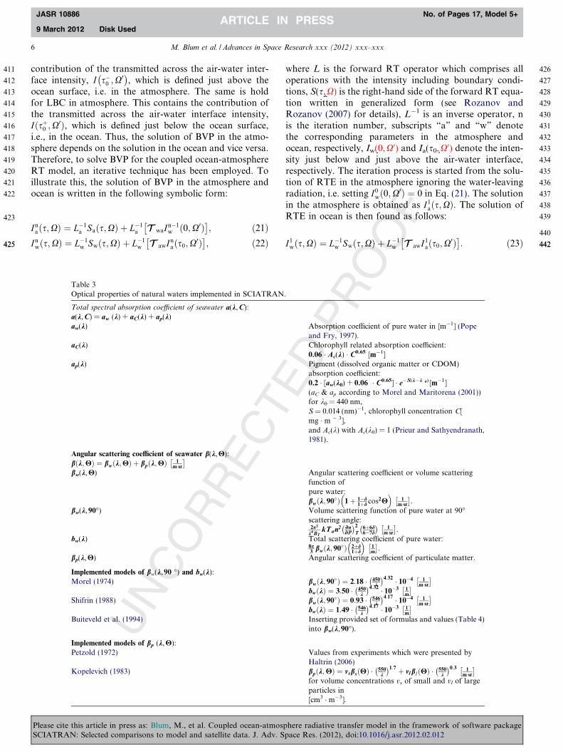
The predictions of SCIATRAN were compared withthose of a number of other models for selected well-definedtest cases, covering specific aspects of the radiative transferin the ocean-atmosphere system as presented by Mobleyet al. (1993). Although seven test problems were definedin the cited above paper we have restricted ourselves tofour following:

1. Optically semi-infinite and vertically homogeneousocean.� Refractive index of water n = 1.34,� Flat ocean-atmosphere interface,� 60� solar zenith angle and E0 = 1 Wm�2 nm�1 inci-

dent solar irradiance,� Black sky,� Pure water scattering described by Rayleigh phase

function,� Single scattering albedo values x0 = 0.2 and

x0 = 0.9.

2. The same as 1 but more realistic Petzold phase functionis used instead of Rayleigh one.

3. The same as 2 but for the vertically stratified ocean.4. The same as 2 but including atmospheric effects.

The following radiative quantities were involved in thecomparison study:

EdðsÞ ¼ l0E0T Fðl0Þe�s=l00 þ 2p

Z 1

0

I0ðs; lÞldl; ð24Þ

E0uðsÞ ¼ 2pZ 0

�1

I0ðs; lÞdl; LuðsÞ ¼ I0ðs;�1Þ; ð25Þ

where Ed(s), E0u(s) and Lu(s) are the total downward irra-diance, upward scalar irradiance and upward nadir radi-ance, respectively, at the optical depth s, I0(s,l) is theazimuthally averaged intensity, l0 and l00 are cosines ofthe solar zenith angle in the atmosphere and ocean, respec-tively, TF(l0) is the Fresnel transmission coefficient.

These radiative quantities were calculated for test prob-lems listed above employing seven RT models (see Mobleyet al. (1993) for details). The discussion of these models isout scope of this paper because it will be used here the aver-age values and standard deviations only which characterizethe variability of results obtained with involved in the com-parison study RT codes. Recently the solution of the firstthree test problems has been obtained also by other RTmodels. In particular, these test problems were solvedemploying matrix operator method (MOMO, Fell andFischer, 2001), finite-element method (FEM, Bulgarelli etal., 1999), and invariant embedding method (demo versionof HydroLight 5.1, Mobley and Sundman, 2008a; Mobleyand Sundman, 2008b). This motivates our choice of threefirst test problems for inter-comparisons. Let us considerall results obtained. Calculated values of Ed, E0u, and Lu



Original text:

Inserted Text

(Θ)

Original text:

Inserted Text

(Θ)

Original text:

Inserted Text

were

Original text:

Inserted Text

ocean

Original text:

Inserted Text

refractive

Original text:

Inserted Text

flat

Original text:

Inserted Text

black

Original text:

Inserted Text

pure

Original text:

Inserted Text

single

Original text:

Inserted Text

),E

Original text:

Inserted Text

Fischer (2001)

Original text:

Inserted Text

al. (1999)

Original text:

Inserted Text

Sundman (2008a),

Original text:

Inserted Text

Sundman (2008b)

547

548

549

550

551

552

553

554

555

556

557

558

559

560

561

562

563

564

565

566

567

568

569

570

571

572

573




alone with average values and standard deviations given byMobley et al. (1993) are summarized in Tables 5 and 6 fortest problems 1 and 2. Results are given at three opticaldepths (s = 1,5,10) and two single scattering albedo(x0 = 0.2,0.9). It follows that HydroLight, SCIATRAN,and MOMO results are very close to each other and standwithin the standard deviations given by Mobley et al.(1993). We recall that the standard deviations indicatethe variability of results obtained with codes involved inthe comparison study by Mobley et al. (1993). It can beseen also that the relative deviations increase with thedecreasing of the single scattering albedo. It can beexplained due to the fact that the increasing of absorption(decreasing of SSA) leads to the significant decreasing of

Table 4General constants and parameters of the volume scattering function accordin

BT Isothermal compressibility of water [Pa�1]

Tc Temperature [�C]P Pressure [Pa]

k ¼ 1:38054 � 10�23 Jð�KÞ

h i

(Boltzmann constant)n Refractive index of water, where refractive index of air

Buiteveld:BT ¼ ð5:062271� 0:03179T c þ 0:000407T 2

cÞ�10�11 [Pa�1] (Lepple and Millero, 1971)

@n@P ¼ @n

@P ðk; T cÞ ¼@n@Pðk;20Þ�@n

@Pð633;T cÞ@n@Pð633;20Þ , where

@n@P ðk; 20Þ ¼ ð�0:000156kþ 1:5989Þ � 10�10

(O’Conner and Schlupf, 1967) function of wavelength, a@n@P ð633; T cÞ ¼ ð1:61857� 0:005785T cÞ � 10�10

(Evtyushenko and Kiyachenko, 1982) function of tempen ¼ 1:3247þ 3:3 � 103 � k�2 � 3:2 � 107 � k�4 � 2:5 � 10�6 � T 2

c(McNeil, 1977) without salinity term

Table 5Results for optically semi-infinite and vertically homogeneous ocean with the

x s HydroLight M

Downward total irradiance Ed

0.2 1 1.412 � 10�1 1.40.2 5 1.057 � 10�3 1.00.2 10 2.956 � 10�6 3.00.9 1 3.660 � 10�1 3.60.9 5 4.309 � 10�2 4.30.9 10 3.109 � 10�3 3.1

Upward scalar irradiance E0u

0.2 1 1.337 � 10�2 1.30.2 5 9.866 � 10�5 9.90.2 10 2.643 � 10�7 2.60.9 1 3.727 � 10�1 3.70.9 5 4.338 � 10�2 4.30.9 10 3.123 � 10�3 3.1

Upward nadir radiance Lu

0.2 1 1.675 � 10�3 1.70.2 5 1.262 � 10�5 1.20.2 10 3.573 � 10�8 3.70.9 1 4.874 � 10�2 4.80.9 5 5.744 � 10�3 5.70.9 10 4.144 � 10�4 4.2


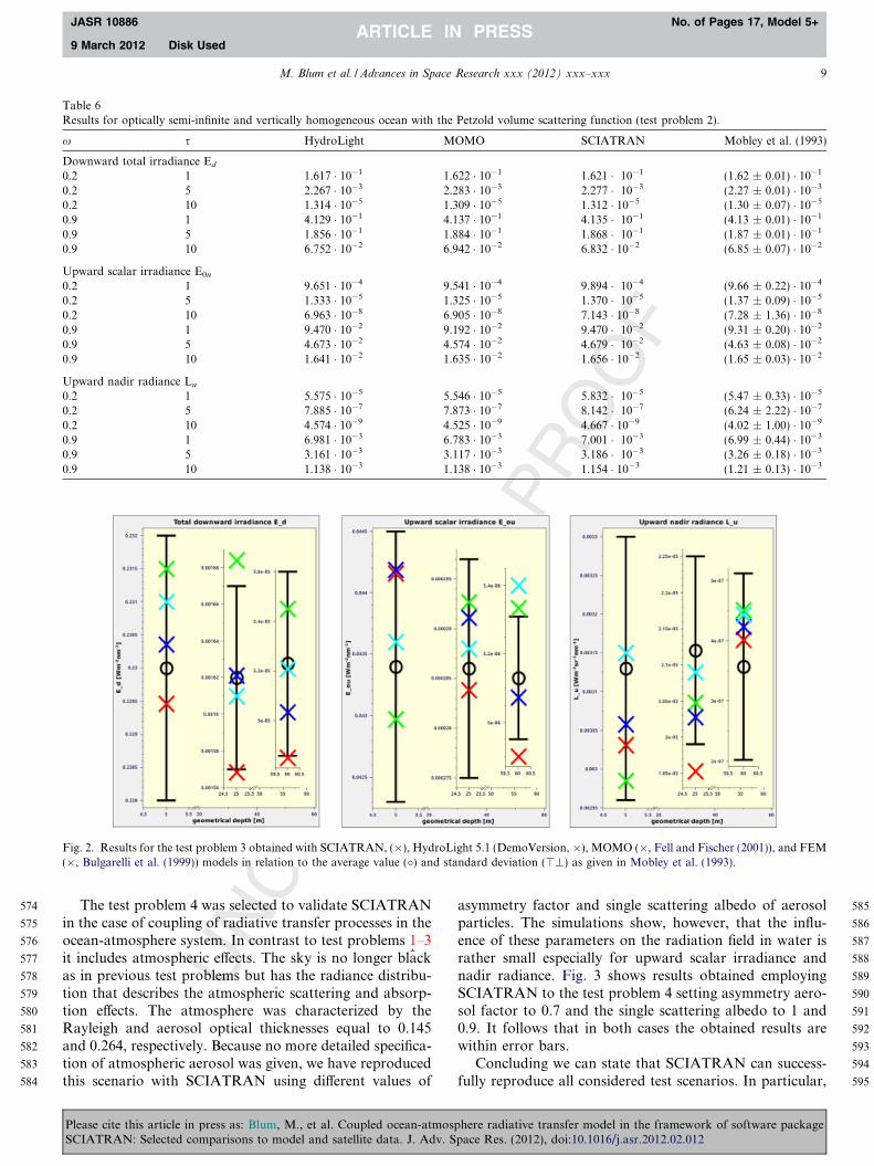
irradiance and especially of upward nadir radiance. Resultsobtained for the test problem 3 are summarized in Fig. 2and Table 7. In this test problem the single scatteringalbedo is assumed to be strongly dependent on the depth(see Mobley et al., 1993 for further details). It can be seenfrom Fig. 2 that for this more complicated test problem theSCIATRAN predictions are within the error bars for alldepth under consideration. In particular, it follows frommiddle panel of Fig. 2 that for the upward scalar irradiance(E0u) at the geometrical depth 60 m only SCIATRANresult is within the error bars (Mobley et al., 1993). Exceptfor this specific depth, the FEM model results (Bulgarelliet al., 1999) are within the error bars also.

g to Buiteveld et al. (1994).

d Depolarization ratio

Ta Absolute temperature [�K]@n@P Pressure derivative of n [Pa�1]

S Spectral slope parameter 1nm

� �

is set to 1

d = 0.051(Farinato and Roswell, 1976)

nd

rature.

Rayleigh volume scattering function (test problem 1).

OMO SCIATRAN Mobley et al. (1993)

15 � 10�1 1.415 � 10�1 (1.41 ± 0.01) � 10�1

66 � 10�3 1.066 � 10�3 (1.07 ± 0.01) � 10�3

27 � 10�6 3.029 � 10�6 (2.93 ± 0.30) � 10�6

65 � 10�1 3.660 � 10�1 (3.66 ± 0.01) � 10�1

34 � 10�2 4.329 � 10�2 (4.33 ± 0.02) � 10�2

50 � 10�3 3.147 � 10�3 (3.16 ± 0.05) � 10�3

36 � 10�2 1.339 � 10�2 (1.34 ± 0.01) � 10�2

05 � 10�5 9.924 � 10�5 (1.00 ± 0.04) � 10�4

90 � 10�7 2.696 � 10�7 (3.00 ± 0.92) � 10�7

26 � 10�1 3.727 � 10�1 (3.72 ± 0.02) � 10�1

51 � 10�2 4.354 � 10�2 (4.35 ± 0.04) � 10�2

55 � 10�3 3.158 � 10�3 (3.20 ± 0.12) � 10�3

06 � 10�3 1.706 � 10�3 (1.72 ± 0.08) � 10�3

96 � 10�5 1.296 � 10�5 (1.37 ± 0.39) � 10�5

53 � 10�8 3.755 � 10�8 (3.39 ± 0.67) � 10�8

81 � 10�2 4.879 � 10�2 (4.85 ± 0.08) � 10�2

84 � 10�3 5.783 � 10�3 (5.59 ± 0.29) � 10�3

04 � 10�4 4.205 � 10�4 (4.37 ± 0.40) � 10�4



Original text:

Inserted Text

1,5,10)

Original text:

Inserted Text

0.2,0.9).

Original text:

Inserted Text

al. (1993)

Original text:

Inserted Text

60m

574

575

576

577

578

579

580

581

582

583

584

585

586

587

588

589

590

591

592

593

594

595

Table 6Results for optically semi-infinite and vertically homogeneous ocean with the Petzold volume scattering function (test problem 2).

x s HydroLight MOMO SCIATRAN Mobley et al. (1993)


0.2 1 1.617 � 10�1 1.622 � 10�1 1.621 � 10�1 (1.62 ± 0.01) � 10�1

0.2 5 2.267 � 10�3 2.283 � 10�3 2.277 � 10�3 (2.27 ± 0.01) � 10�3

0.2 10 1.314 � 10�5 1.309 � 10�5 1.312 � 10�5 (1.30 ± 0.07) � 10�5

0.9 1 4.129 � 10�1 4.137 � 10�1 4.135 � 10�1 (4.13 ± 0.01) � 10�1

0.9 5 1.856 � 10�1 1.884 � 10�1 1.868 � 10�1 (1.87 ± 0.01) � 10�1

0.9 10 6.752 � 10�2 6.942 � 10�2 6.832 � 10�2 (6.85 ± 0.07) � 10�2


0.2 1 9.651 � 10�4 9.541 � 10�4 9.894 � 10�4 (9.66 ± 0.22) � 10�4

0.2 5 1.333 � 10�5 1.325 � 10�5 1.370 � 10�5 (1.37 ± 0.09) � 10�5

0.2 10 6.963 � 10�8 6.905 � 10�8 7.143 � 10�8 (7.28 ± 1.36) � 10�8

0.9 1 9.470 � 10�2 9.192 � 10�2 9.470 � 10�2 (9.31 ± 0.20) � 10�2

0.9 5 4.673 � 10�2 4.574 � 10�2 4.679 � 10�2 (4.63 ± 0.08) � 10�2

0.9 10 1.641 � 10�2 1.635 � 10�2 1.656 � 10�2 (1.65 ± 0.03) � 10�2


0.2 1 5.575 � 10�5 5.546 � 10�5 5.832 � 10�5 (5.47 ± 0.33) � 10�5

0.2 5 7.885 � 10�7 7.873 � 10�7 8.142 � 10�7 (6.24 ± 2.22) � 10�7

0.2 10 4.574 � 10�9 4.525 � 10�9 4.667 � 10�9 (4.02 ± 1.00) � 10�9

0.9 1 6.981 � 10�3 6.783 � 10�3 7.001 � 10�3 (6.99 ± 0.44) � 10�3

0.9 5 3.161 � 10�3 3.117 � 10�3 3.186 � 10�3 (3.26 ± 0.18) � 10�3

0.9 10 1.138 � 10�3 1.138 � 10�3 1.154 � 10�3 (1.21 ± 0.13) � 10�3

Fig. 2. Results for the test problem 3 obtained with SCIATRAN, (�), HydroLight 5.1 (DemoVersion, �), MOMO (�, Fell and Fischer (2001)), and FEM(�, Bulgarelli et al. (1999)) models in relation to the average value (�) and standard deviation (>\) as given in Mobley et al. (1993).




The test problem 4 was selected to validate SCIATRANin the case of coupling of radiative transfer processes in theocean-atmosphere system. In contrast to test problems 1–3it includes atmospheric effects. The sky is no longer blackas in previous test problems but has the radiance distribu-tion that describes the atmospheric scattering and absorp-tion effects. The atmosphere was characterized by theRayleigh and aerosol optical thicknesses equal to 0.145and 0.264, respectively. Because no more detailed specifica-tion of atmospheric aerosol was given, we have reproducedthis scenario with SCIATRAN using different values of


asymmetry factor and single scattering albedo of aerosolparticles. The simulations show, however, that the influ-ence of these parameters on the radiation field in water israther small especially for upward scalar irradiance andnadir radiance. Fig. 3 shows results obtained employingSCIATRAN to the test problem 4 setting asymmetry aero-sol factor to 0.7 and the single scattering albedo to 1 and0.9. It follows that in both cases the obtained results arewithin error bars.

Concluding we can state that SCIATRAN can success-fully reproduce all considered test scenarios. In particular,



Original text:

Inserted Text

1-3

596

597

598

599

600

601

602

603

604

605

606

608608

609

610

611

612

613

614

615

616

617

618

619

620

621

622

623

624

625

626

627

628

Table 7Results for the vertically inhomogeneous ocean (test problem 3).

z [m] HydroLight MOMO SCIATRAN Bulgarelli Mobley et al. (1993)


5 2.295 � 10�1 2.315 � 10�1 2.304 � 10�1 2.31 � 10�1 (2.30 ± 0.02) � 10�1

25 1.568 � 10�3 1.684 � 10�3 1.621 � 10�3 1.61 � 10�3 (1.62 ± 0.05) � 10�3

60 4.851 � 10�5 5.451 � 10�5 5.035 � 10�5 5.21 � 10�5 (5.23 ± 0.37) � 10�5


5 4.416 � 10�2 4.297 � 10�2 4.419 � 10�2 4.36 � 10�2 (4.34 ± 0.11) � 10�2

25 2.838 � 10�4 2.927 � 10�4 2.911 � 10�4 2.88 � 10�4 (2.86 ± 0.11) � 10�4

60 4.901 � 10�6 5.334 � 10�6 5.073 � 10�6 5.40 � 10�6 (5.13 ± 0.18) � 10�6


5 3.031 � 10�3 2.985 � 10�3 3.058 � 10�3 3.15 � 10�3 (3.13 ± 0.17) � 10�3

25 1.953 � 10�5 2.048 � 10�5 2.028 � 10�5 2.09 � 10�5 (2.12 ± 0.13) � 10�5

60 4.014 � 10�7 4.508 � 10�7 4.229 � 10�7 4.43 � 10�7 (3.57 ± 1.55) � 10�7

Fig. 3. Results for the test problem 4 obtained with the SCIATRAN model setting asymmetry factor and single scattering albedo of aerosol to 0.7 and 1.0(�), and to 0.7 and 0.9 (+) in relation to the average value (�) and error bar (>\) as given in Mobley et al. (1993).




test problems 1–3 demonstrate that the implementation ofuncoupled oceanic RT model in the software packageSCIATRAN is correct. The solution of the test problem4 shows that in the considered case the impact of thecoupling on the light field within water is not too much.

4.2. Comparison to MERIS measurements

Comparisons of spectra calculated with SCIATRANand measured by MERIS were performed for the reflec-tance at the top of atmosphere (reftoa). The reflectance isdefined as follows:

Rð#;u; kÞ ¼ pIð#;u; kÞE0ðkÞ cos#0

; ð26Þ

where I(#,u,k) is the radiance at given zenith # and azi-muthal u angles, E0(k) is the extraterrestrial solar spectralirradiance, k is the wavelength, and #0 denotes the sun


zenith angle. We have used the reflectance for comparisonsof model and experimental data because it does not containany additional systematical errors caused by employingatmospheric correction techniques that are usually usedto obtain water-leaving radiance.

To calculate R(#,u,k) one needs to define all relevantatmospheric and oceanic parameters. In particular, the fol-lowing parameters are required:

� MERIS data have been used to define the observationgeometry, the solar zenith angle, the atmospheric pres-sure, the concentrations of H2O and O3, the aerosoloptical thickness at 550 and 865 nm, and the geograph-ical position of measurement points;� AERONET data (http://aeronet.gsfc.nasa.gov/) have

been used to obtain the aerosol phase function, the aer-osol extinction coefficient, and the aerosol single scatter-ing albedo at 440, 675, 870, and 1020 nm;


http://aeronet.gsfc.nasa.gov/


Original text:

Inserted Text

1-3

629

630

631

632

633

634

635

636

637

638

639

640

641

642

643

644

645

646

647

648

649

650

651

652

653

654

655

656

657

658

659

660

661

662

663

664

665

666

667

668

669

670

671

672

673

674

675

676




� ocean parameters such as temperature, salinity, chloro-phyll concentration, and concentrations of small andlarge particles at different depths were obtained fromthe BOUSSOLE data (BOUSSOLE boy at 43.6�E,7.8�N; see Antoine et al., 2008);� the reflection and transmission properties of the ocean

surface were defined by the Gaussian surface slopePDF (including shadowing effects) and the mean squareslope as given by Cox and Munk (1954), Cox and Munk(1954), the pure seawater and hydrosol volume scatter-ing functions were used according to Buiteveld et al.(1994) and Kopelevich (1983) models, respectively.

In order to perform comparisons, MERIS data suitablefor the comparison with model calculations were matchedto co-located AERONET and BOUSSOLE measurementsites. Moreover, the time difference between measurementsperformed by the MERIS instrument, AERONET, andBOUSSOLE data was kept as small as possible, since timedifferences between the different measurements up to 10hours occured. There are some additional criteria bychoosing the MERIS data for the comparison, e.g. cloudyscenes and the observation geometry near to the solar glinthave to be avoided. Taking into account all of the above

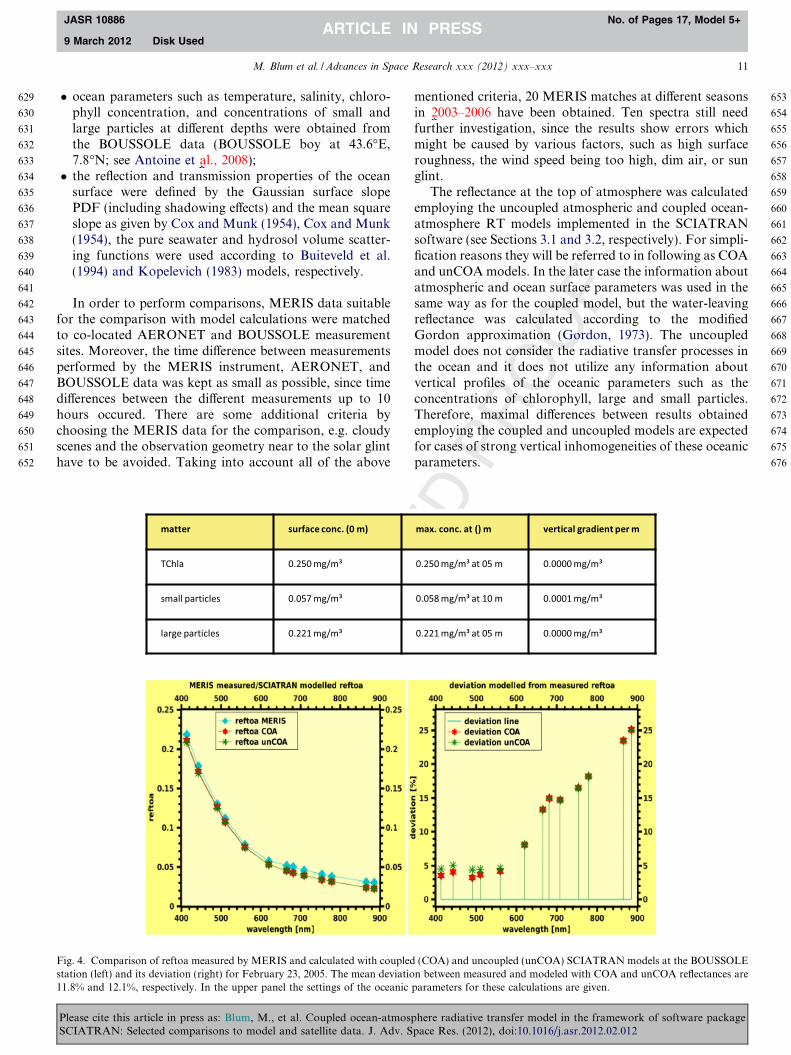
Fig. 4. Comparison of reftoa measured by MERIS and calculated with coupledstation (left) and its deviation (right) for February 23, 2005. The mean deviatio11.8% and 12.1%, respectively. In the upper panel the settings of the oceanic


mentioned criteria, 20 MERIS matches at different seasonsin 2003–2006 have been obtained. Ten spectra still needfurther investigation, since the results show errors whichmight be caused by various factors, such as high surfaceroughness, the wind speed being too high, dim air, or sunglint.

The reflectance at the top of atmosphere was calculatedemploying the uncoupled atmospheric and coupled ocean-atmosphere RT models implemented in the SCIATRANsoftware (see Sections 3.1 and 3.2, respectively). For simpli-fication reasons they will be referred to in following as COAand unCOA models. In the later case the information aboutatmospheric and ocean surface parameters was used in thesame way as for the coupled model, but the water-leavingreflectance was calculated according to the modifiedGordon approximation (Gordon, 1973). The uncoupledmodel does not consider the radiative transfer processes inthe ocean and it does not utilize any information aboutvertical profiles of the oceanic parameters such as theconcentrations of chlorophyll, large and small particles.Therefore, maximal differences between results obtainedemploying the coupled and uncoupled models are expectedfor cases of strong vertical inhomogeneities of these oceanicparameters.

(COA) and uncoupled (unCOA) SCIATRAN models at the BOUSSOLEn between measured and modeled with COA and unCOA reflectances are

parameters for these calculations are given.



Original text:

Inserted Text

al. (2008)

Original text:

Inserted Text

2003 - 2006

677

678

679

680

681

682

683

684

685

686

687

688

689

690

691

692

693

694

695

696

697

698

699

700

701

702

703

704

705

706

707

708

709

710

711

712

713

714

715

716

717

718

719

720

721

722

723

724

725

726

727




The preliminary analysis of all results obtained showsthat indeed in the case of almost vertically homogeneousocean both models produce very similar results. In partic-ular, Fig. 4 shows, as an example, the comparison of mod-elled reflectance with the MERIS measurement performedin February 23, 2005, in the case of low varying with depthchlorophyll and particulate matter concentrations. Bothmodels describe in this case the measured reflectance spec-tra with a similar accuracy.

Figs. 5 and 6 show the comparison of modelled reflec-tances with the MERIS measurements performed in April5, 2003, and in July 31, 2004, respectively. According tothe BOUSSOLE data, the vertical profiles of chlorophyllconcentration show very similar vertical gradients(�0.027 mg � m�3/m) for both days, but the chlorophyllconcentration at the ocean surface was more than threetimes larger in April than in July. Comparing results pre-sented in Figs. 5 and 6, we can conclude that for both daysthe coupled model shows better coincidence with theMERIS spectra in the spectral range relevant to the chloro-phyll absorption (400–560 nm), where pure seawaterabsorption is low. Furthermore, Fig. 7 (October 5, 2006)demonstrates the impact of the vertical gradient of thechlorophyll concentration on the performance of the cou-pled and uncoupled models. Using the BOUSSOLE data,the vertical gradient of the chlorophyll concentration was

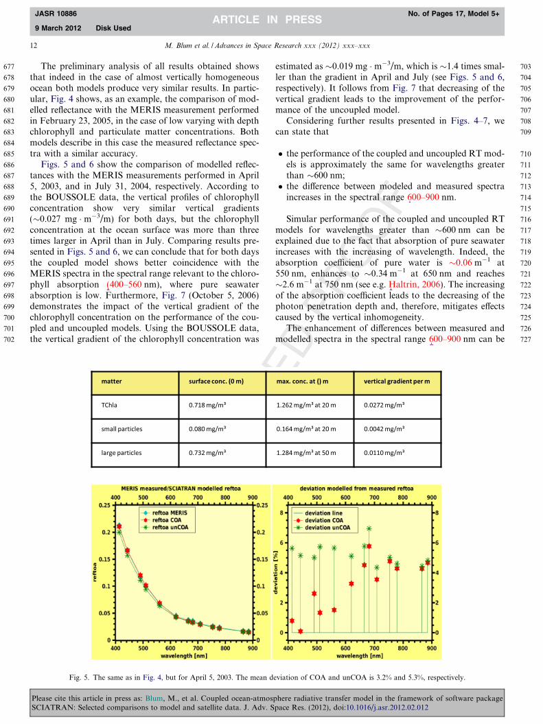
Fig. 5. The same as in Fig. 4, but for April 5, 2003. The mean d


estimated as �0.019 mg � m�3/m, which is �1.4 times smal-ler than the gradient in April and July (see Figs. 5 and 6,respectively). It follows from Fig. 7 that decreasing of thevertical gradient leads to the improvement of the perfor-mance of the uncoupled model.

Considering further results presented in Figs. 4–7, wecan state that

� the performance of the coupled and uncoupled RT mod-els is approximately the same for wavelengths greaterthan �600 nm;� the difference between modeled and measured spectra

increases in the spectral range 600–900 nm.

Simular performance of the coupled and uncoupled RTmodels for wavelengths greater than �600 nm can beexplained due to the fact that absorption of pure seawaterincreases with the increasing of wavelength. Indeed, theabsorption coefficient of pure water is �0.06 m�1 at550 nm, enhances to �0.34 m�1 at 650 nm and reaches�2.6 m�1 at 750 nm (see e.g. Haltrin, 2006). The increasingof the absorption coefficient leads to the decreasing of thephoton penetration depth and, therefore, mitigates effectscaused by the vertical inhomogeneity.

The enhancement of differences between measured andmodelled spectra in the spectral range 600–900 nm can be

eviation of COA and unCOA is 3.2% and 5.3%, respectively.



Original text:

Inserted Text

(400 - 560

Original text:

Inserted Text

600-900

Original text:

Inserted Text

Haltrin (2006)

Original text:

Inserted Text

600-900

728

729

730

731

732

733

734

735

736

737

738

739

740

741

742

743

744

745

746

747

748

749

750

751

752

753

754

755

756

757

758

759

760

761

762

763

764

765

766

767

768

769

770

771

772

773

774

775

776

777

Fig. 6. The same as in Fig. 4, but for July 31, 2004. The mean deviation of COA and unCOA is 6.2% and 7.5%, respectively.




explained by the ignoring of inelastic scattering processessuch as vibrational Raman scattering and fluorescence inthe current version of our RT model. However, a morerealistic reason of this difference can be the lack of exactinformation on atmospheric aerosol parameters.

5. Conclusion

We have discussed the theoretical background of radia-tive transfer processes and inherent optical parameters ofthe natural water implemented in the extended version ofthe software package SCIATRAN. The extended SCIA-TRAN versions 3.1 and greater allow users to accountfor not only the radiative processes within the atmospherebut also within the ocean including they interaction.

Taking into account that the atmospheric radiativetransfer of the SCIATRAN software has been successfullyvalidated (Kokhanovsky et al., 2010), we have presentedhere the validation of the oceanic radiative transfer. Com-parisons of SCIATRAN results to the predictions of otherRT models used to solve selected well-defined test prob-lems, covering specific aspects of the radiative transfer inthe ocean-atmosphere system (Mobley et al., 1993), havedemonstrated good performance of the extended SCIA-TRAN version to calculate the radiative transfer withinwater. In order to establish that all physical processes are


properly incorporated to describe radiative processes inthe coupled ocean-atmosphere system we have presentedcomparisons of the model predictions with measurementsperformed by MERIS instrument. Comparisons showgood agreement between measured and modeled reflec-tances in the spectral range 400–550 nm where the couplingeffects are significant. This demonstrates that the extendedSCIATRAN version can be employed to model satellitemeasurements of the reflected radiation performed overoceanic sites properly accounting for the vertical distribu-tion of oceanic parameters. The contribution of thewater-leaving radiance into the final detected signal is atmaximum approximately 10% to the backscattered radi-ance measured by the satellite sensor. Therefore, the accu-racy of the RT modeling at the top of the atmosphereradiation should not exceed more than one to two percent.Also for atmospheric retrievals of trace gases accuracywithin a few percent is needed. This also requires thatRT modeling is done at high spectral resolution as it is pro-vided by SCIATRAN.

We have demonstrated also that employing the uncou-pled atmospheric RT model to simulate satellite measure-ments of the reflected radiation over the oceanic sites canlead to systematic errors in the spectral range 400–550 nm. These error are caused by the vertical inhomogene-ity of the inherent optical parameters and can be significant



Original text:

Inserted Text

400-550

Original text:

Inserted Text

400-550

778

779

780

781

782

783

784

785

786

787

788

789

790

791

792

793

794

795

796

797

798

799

800

801

802

803

804

805

806

807

808

809

810

811

812

813

814

815

816

817

818

819

820

821

822

823

824

825

826

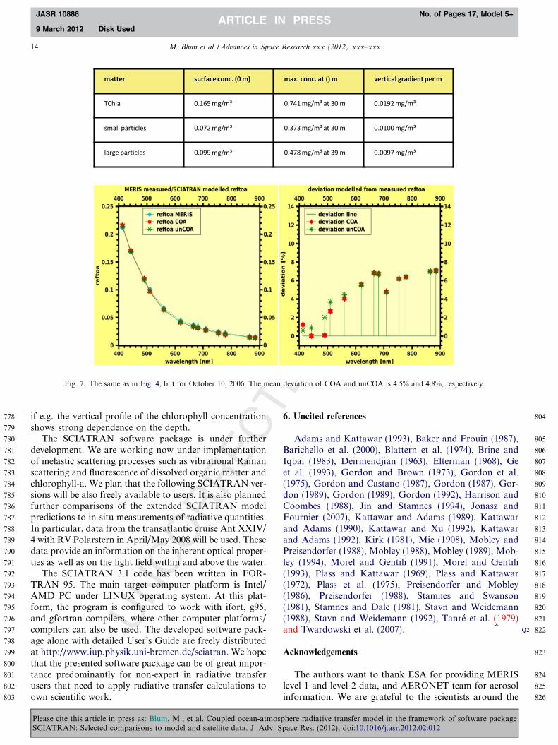
Fig. 7. The same as in Fig. 4, but for October 10, 2006. The mean deviation of COA and unCOA is 4.5% and 4.8%, respectively.

Q2




if e.g. the vertical profile of the chlorophyll concentrationshows strong dependence on the depth.

The SCIATRAN software package is under furtherdevelopment. We are working now under implementationof inelastic scattering processes such as vibrational Ramanscattering and fluorescence of dissolved organic matter andchlorophyll-a. We plan that the following SCIATRAN ver-sions will be also freely available to users. It is also plannedfurther comparisons of the extended SCIATRAN modelpredictions to in-situ measurements of radiative quantities.In particular, data from the transatlantic cruise Ant XXIV/4 with RV Polarstern in April/May 2008 will be used. Thesedata provide an information on the inherent optical proper-ties as well as on the light field within and above the water.

The SCIATRAN 3.1 code has been written in FOR-TRAN 95. The main target computer platform is Intel/AMD PC under LINUX operating system. At this plat-form, the program is configured to work with ifort, g95,and gfortran compilers, where other computer platforms/compilers can also be used. The developed software pack-age alone with detailed User’s Guide are freely distributedat http://www.iup.physik.uni-bremen.de/sciatran. We hopethat the presented software package can be of great impor-tance predominantly for non-expert in radiative transferusers that need to apply radiative transfer calculations toown scientific work.


6. Uncited references

Adams and Kattawar (1993), Baker and Frouin (1987),Barichello et al. (2000), Blattern et al. (1974), Brine andIqbal (1983), Deirmendjian (1963), Elterman (1968), Geet al. (1993), Gordon and Brown (1973), Gordon et al.(1975), Gordon and Castano (1987), Gordon (1987), Gor-don (1989), Gordon (1989), Gordon (1992), Harrison andCoombes (1988), Jin and Stamnes (1994), Jonasz andFournier (2007), Kattawar and Adams (1989), Kattawarand Adams (1990), Kattawar and Xu (1992), Kattawarand Adams (1992), Kirk (1981), Mie (1908), Mobley andPreisendorfer (1988), Mobley (1988), Mobley (1989), Mob-ley (1994), Morel and Gentili (1991), Morel and Gentili(1993), Plass and Kattawar (1969), Plass and Kattawar(1972), Plass et al. (1975), Preisendorfer and Mobley(1986), Preisendorfer (1988), Stamnes and Swanson(1981), Stamnes and Dale (1981), Stavn and Weidemann(1988), Stavn and Weidemann (1992), Tanre et al. (1979)and Twardowski et al. (2007).

Acknowledgements

The authors want to thank ESA for providing MERISlevel 1 and level 2 data, and AERONET team for aerosolinformation. We are grateful to the scientists around the




Original text:

Inserted Text

(1979),

827

828

829

830

831

832

833834835836837838839840841842843844845846847848849850851852853854855856857858859860861862863864865866867868869870871872873874875876877878879880881882883884885886887888889890

891892893894895896897898899900901902903904905906907908909910911912913914915916917918919920921922923924925926927928929930931932933934935936937938939940941942943944945946947948949950951952953954955956957958




BOUSSOLE project, especially to the director David An-toine for providing BOUSSOLE in-situ data. This workhas in part been funded by HGF & AWI (projects PHY-TOOPTICS and ESSReS), German Aerospace Center(DLR), University and State of Bremen.

References

Adams, C., Kattawar, G. Effect of volume scattering function on theerrors induced when polarization is neglected in radiance calculationsin an atmosphere-ocean system. Appl. Opt. 20, 4610–4617, 1993.

Anikonov, A.S., Ermolaev, S.Y. On diffuse light reflection from asemiinfinite atmosphere with a highly extended phase function. VestnikLGU 7, 132–137, 1977.

Antoine, D., d’Ortenzio, F., Hooker, S.B., Becu, G., Gentili, B., Taillez,D., Scott, A.J. Assessment of uncertainty in the ocean reflectancedetermined by three satellite ocean color sensors (MERIS, SeaWiFSand MODIS-A) at an offshore site in the Mediterranean Sea(BOUSSOLE project). J. Geophys. Res. 113, C07013, doi:10.1029/2007JC004472, 2008.

Baker, K., Frouin, R. Relation between photosynthetically availableradiation and total insolation at the ocean surface under clear skies.Limnol. Oceanogr. 32, 1370–1377, 1987.

Barichello, L.B., Garcia, R.D.M., Siewert, C.E. Particular solutions forthe discrete-ordinates method. J. Quant. Spectr. Radiat. Transfer 64,219–226, 2000.

Bezy, J.L., Delwart, S., Rast, M. MERIS – A new generation of ocean-colour sensor onboard envisat. ESA Bull. 103, 48–56, 2000.

Blattern, W., Horak, H., Collins, D., Wells, M. Monte Carlo studies of thesky radiation at twilight. Appl. Opt. 13, 534, 1974.

Born, M., Wolf, E. Principles of Optics, 2nd ed Pergamon press, Oxford,London, Edinburgh, New York, Paris, Frankfurt, 1964.

Bovensmann, H., Burrows, J.P., Buchwitz, M., Frerick, J., Noel, S.,Rozanov, V.V., Chance, K.V., Goede, A.P.H. SCIAMACHY: Missionobjectives and measurement modes. J. Atmos. Sci. 56, 127–149, 1999.

Bracher, A., Vountas, M., Dinter, T., Burrows, J.P., Roettgers, R.,Peeken, I. Quantitative observation of cyanobacteria and diatomsfrom space using PhytoDOAS on SCIAMACHY data. Biogeosciences6, 751–764, 2009.

Brine, D., Iqbal, M. Diffuse and global solar spectral irradiance undercloudless skies. Sol. Energy 30, 447–453, 1983.

Buiteveld, H., Hakvoort, J.H.M., Donze, M. The optical properties ofpure water. SPIE Ocean Optics XII 2258, 174–183, 1994.

Bulgarelli, B., Kisselev, V., Roberti, L. Radiative transfer in theatmosphere-ocean system: the finite-element method. Appl. Opt. 38,1530–1542, 1999.

Chandrasekhar, S. Radiative Transfer. Oxford University Press, London,1950.

Cox, C., Munk, W. Measurement of the roughness of the sea surface fromphotographs of the suns glitter. J. Opt. Soc. Am. 44 (11), 838–850, 1954.

Cox, C., Munk, W. Statistics of the sea surface derived from sun glitter. J.Marine Res. 13 (2), 198–227, 1954.

Deirmendjian, D. Scattering and polarization properties of polydispersesuspensions with partial absorption, in: Kerker, M. (Ed.), Electro-magnetic Scattering. Pergamon, New York, pp. 171–189, 1963.

Elterman, L., UV, visible, and IR attenuation for altitudes to 50 km,Report. AFCRL-68-0153, U.S. Air Force Cambridge Research Lab-oratory, Bedford, Mass, 1968.

Evtyushenko, A.M., Kiyachenko, Y.F. Determination of the dependenceof liquid refractive index on pressure and temperature. Opt. Spectrosc.52, 56–58, 1982.

Farinato, R.S., Roswell, R.L. New values of the light scattering depolar-ization and anisotropy of water. J. Chem. Phys. 65, 593–595, 1976.

Fell, F., Fischer, J. Numerical simulation of the light field in theatmosphere-ocean system using the matrix-operator method. J. Quant.Spectr. Radiat. Transfer 69, 351–388, 2001.


Ge, Y., Gordon, H.R., Voss, K. Simulation of inelastic- scatteringcontributions to the irradiance field in the oceanic variation inFraunhofer line depths. Appl. Opt. 32, 4028–4036, 1993.

Gordon, H.R., Brown, O. Irradiance reflectivity of a flat ocean as afunction of its optical properties. Appl. Opt. 12, 1549–1551, 1973.

Gordon, H.R. Simple calculation of the diffuse reflectance of the ocean.Appl. Opt. 12 (12), 2803–2804, 1973.

Gordon, H.R., Brown, O., Jacobs, M. Computed relationships betweenthe inherent and apparent optical properties of a flat homogeneousocean. Appl. Opt. 14, 417–427, 1975.

Gordon, H.R., Castano, D. Coastal zone color scanner atmosphericcorrection algorithm: multiple scattering effects. Appl. Opt. 26, 2111,1987.

Gordon, H.R. A bio-optical model describing the distribution ofirradiance at the sea surface resulting from a point source embeddedin the ocean. Appl. Opt. 26, 4133–4148, 1987.

Gordon, H.R. Can the Lambert-Beer law be applied to the diffuseattenuation coefficient of ocean water? Limnol. Oceanogr. 34, 1389–1409, 1989.

Gordon, H.R. Dependence of the diffuse reflectance of natural waters onthe sun angle. Limnol. Oceanogr. 34, 1484–1489, 1989.

Gordon, H.R. Diffuse reflectance of the ocean: influence of nonuniformphytoplankton pigment profile. Appl. Opt. 31, 2116–2129, 1992.

Gottwald, M. SCIAMACHY, Monitoring the Changing Earth’s Atmo-sphere, DLR. Institute fuer Methodik der Fernerkundung, 2006.

Haltrin, V.I. Absorption and scattering of light in natural waters, in:Kokhanovsky, A.A. (Ed.), Light Scattering Reviews. Springer, PraxisPublishing, Chichester, UK, pp. 445–486, 2006.

Harrison, A., Coombes, C. Angular distribution of clear sky shortwavelength radiance. Sol. Energy 40, 57–69, 1988.

He, Xianqiang, Bai, Yan, Zhu, Qiankun, Gong, Fang A vector radiativetransfer model of coupled oceanatmosphere system using matrix-operator method for rough sea-surface. J. Quant. Spectr. Radiat.Transfer 111, 1426–1448, doi:10.1016/j.jqsrt.2010.02.014, 2010.

Jin, Z., Stamnes, K. Radiative transfer in nonuniformly refracting layeredmedia: atmosphere-ocean system. Appl. Opt. 33 (3), 431–442, 1994.

Jin, Z., Charlock, T.P., Rutledge, K., Stamnes, K., Wang, Y. Analyticalsolution of radiative transfer in the coupled atmosphere ocean systemwith a rough surface. Appl. Opt. 45 (28), 7443–7455, 2006.

Jonasz, M., Fournier, G.R. Light Scattering by Particles in Water.Theoretical and Experimental Foundations. Academic Press, ElsevierInc, 2007.

Kattawar, G., Adams, C. Stokes vector calculations of the submarine lightfield in an atmosphere-ocean with scattering according to a Rayleighphase matrix: effect of interface refractive index on radiance andpolarization. Limnol. Oceanogr. 34, 1453–1472, 1989.

Kattawar, G., Adams, C., Errors in radiance calculations induced by usingscalar rather than Stokes vector theory in a realistic atmosphere-oceansystem, In: Ocean Optics vol. X, (eds.) by R.W. Spinrad, Proc. Soc.Photo-Opt. Instrum. Eng. 1302, pp. 2–12, 1990.

Kattawar, G., Xu, X. Filling-in of Fraunhofer lines in the ocean byRaman scattering. Appl. Opt. 31, 1055–1065, 1992.

Kattawar, G., Adams, C. Errors induced when polarization is neglected inradiance calculations for an atmosphere-ocean system. In: Estep, L.(Ed.), Optics for the Air-Sea Interface: Theory and Measurement.Proc. Soc. Photo-Opt. Instrum. Eng. 1749, pp. 2–22, 1992.

Kirk, J. Monte Carlo procedure for simulating the penetration of lightinto natural waters, Div. Plant Industry Technical Paper 36, Com-monwealth Scientific and Industrial Research Organization, Canberra,Australia, 1981.

Kokhanovsky, A.A., Sokoletsky, L.G. Reflection of light from semi-infinite absorbing turbid media. Part 2: Plane albedo and reflectionfunction. Color Res. Appl. 31, 498–509, 2006.

Kokhanovsky, A.A., Budak, V.P., Cornet, C., Duan, M., Emde, C.,Katsev, I.L., Klyukov D.A., Korkin, S.V., Labonnote, L.C., Min, Q.,Nakajima, T., Ota, Y., Prikhach, A.P., Rozanov, V.V., Yokota, T.,Zege, E.P. Benchmark results in vector atmospheric radiative transfer.J. Quant. Spectr. Radiat. Transfer 111, 1931–1946, 2010.


http://dx.doi.org/10.1029/2007JC004472

http://dx.doi.org/10.1029/2007JC004472

http://dx.doi.org/10.1016/j.jqsrt.2010.02.014


Original text:

Inserted Text

(DLR),

Original text:

Inserted Text

Bremen.

959960961962963964965966967968969970971972973974975976977978979980981982983984985986987988989990991992993994995996997998999

10001001100210031004100510061007100810091010101110121013101410151016101710181019102010211022102310241025

1026102710281029103010311032103310341035103610371038103910401041104210431044104510461047104810491050105110521053105410551056105710581059106010611062106310641065106610671068106910701071107210731074107510761077107810791080108110821083108410851086108710881089109010911092




Kopelevich, O.V. Small-parameter model of optical properties of seawa-ter, in: Monin, A.S. (Ed.), Ocean Optics, Physical ocean optics, vol. 1.Nauka, Moscow (in Russian), pp. 208–234, 1983.

Lepple, F.K., Millero, F.J. The isothermal compressibility of seawaternear one atmosphere. Deep-Sea Res. 18, 1233–1254, 1971.

McNeil, G.T. Metrical fundamentals of underwater lens systems. Opt.Eng. 16, 128–139, 1977.

Mie, G. Beitre zur Optik trber Medien, speziell Kolloidalen Metall-Lsungen. Ann. Phys. 25, 377–445, 1908.

Mobley, C.D., Preisendorfer, R. A numerical model for the computationof radiance distributions in natural waters with wind-roughenedsurfaces, NOAA Tech. Memo. ERL PMEL-75(NTIS PB88-192703),Pacific Marine Environmental Laboratory, Seattle, Wash., 1988.

Mobley, C.D. A numerical model for the computation of radiancedistributions in natural waters with wind-roughened surfaces, part II:user’s guide and code listing, NOAA Tech. Memo. ERL PMEL-81(NTIS PB88-246871), Pacific Marine Environmental Laboratory,Seattle, Wash., 1988.

Mobley, C.D. A numerical model for the computation of radiancedistributions in natural waters with wind-roughened surfaces. Limnol.Oceanogr. 34, 1473–1483, 1989.

Mobley, C.D., Gentili, B., Gordon, H.R., Jin, Z., Kattawar, G.W., Morel,A., Reinersman, P., Stamnes, K., Stavn, R.H. Comparison ofnumerical models for computing underwater light fields. Appl. Opt.32 (36), 7484–7504, 1993.

Mobley, C.D. Light and water. Radiative transfer in natural waters.Academic Press, Inc, 1994.

Mobley, C.D., Sundman, L.K. Hydrolight – Ecolight 5.0 users’ guide,Tech. Rep., Sequoia Scientific, Inc., Bellevue, WA. First PrintingDecember 2008.

Mobley, C.D., Sundman, L.K. Hydrolight – Ecolight 5.0, TechnicalDocumentation. Tech. Rep., Sequoia Scientific, Inc., Bellevue, WA.First Printing December 2008.

Morel, A. Optical properties of pure water and pure seawater, in: Jerlov,N.G., Nielson, E.S. (Eds.), Optical Aspects of Oceanography.Academic, New York, pp. 1–24, 1974.

Morel, A., Gentili, B. Diffuse reflectance of oceanic waters: Its dependenceon Sun angle as influenced by the molecular scattering contribution.Appl. Opt. 30 (30), 4427–4438, 1991.

Morel, A., Gentili, B. Diffuse reflectance of oceanic waters. II. Bidirec-tional aspects. Appl. Opt. 32 (33), 6864–6879, 1993.

Morel, A., Maritorena, S. Bio-optical properties of oceanic waters: areappraisal. J. Geophy. Res. 106 (C4), 7163–7180, 2001.

Nakajima, T., Tanaka, M. Effect of wind generated waves on the transferof solar radiation in the atmosphere-ocean system. J. Quant. Spectr.Radiat. Transfer 29, 521–537, 1983.

O’Conner, C.L., Schlupf, J.P. Brillouin scattering in water: the Landau–Paszek ratio. J. Chem. Phys. 47, 3138, 1967.

Ota, Y., Higurashi, A., Najajima, T., Yokota, T. Matrix formulations ofradiative transfer including the polarization effect in a coupledatmosphere ocean system. J. Quant. Spectr. Radiat. Transfer 111,878–894, 2010.

Petzold, T.J. Volume scattering functions for selected ocean waters, SIORef. 72-78, Scripps Institute of Oceanography, Visibility Laboratory,San Diego, CA, 1972.

Plass, G., Kattawar, G. Radiative transfer in an atmosphere-ocean system.Appl. Opt. 8, 455–466, 1969.

Plass, G., Kattawar, G. Monte-Carlo calculations of radiative transfer inthe earth’s atmosphere ocean system: I. Flux in the atmosphere andocean. J. Phys. Oceanogr. 2, 139–145, 1972.

Plass, G., Kattawar, G., Guinn, J.Jr. Radiative transfer in the earth’satmosphere and ocean: influence of ocean waves. Appl. Opt. 14, 1924–1936, 1975.

Pope, R.M., Fry, E.S. Absorption spectrum (380–700 nm) of pure water:II. Integrating cavity measurements. Appl. Opt. 36, 8710–8723, 1997.

Preisendorfer, R., Mobley, C.D. Albedos and glitter patterns of a wind-roughened sea surface. J. Phys. Oceanogr. 16, 1293–1316, 1986.

1093


Preisendorfer, R. Eigenmatrix representations of radiance distributions inlayered natural waters with wind-roughened surfaces, NOAA Tech.Memo. ERL PMEL-76(NTIS PB88-188701), Pacific Marine Environ-mental Laboratory, Seattle, Wash., 1988.

Prieur, L., Sathyendranath, S. An optical classification of coastal andoceanic waters based on the specific absorption curves of phytoplank-ton pigments, dissolved organic matter, and other particulate mate-rials. Limnol. Oceanogr. 26, 671–689, 1981.

Rozanov, A. SCIATRAN 2.X: Radiative transfer model and retrievalsoftware package, <http://www.iup.uni-bremen.de/sciatran/>, 2008.

Rozanov, V.V., Rozanov, A.V. Generalized form of the direct and adjointradiative transfer equations. J. Quant. Spectr. Radiat. Transfer 104,155–170, 2007.

Rozanov, A., Rozanov, V.V., Buchwitz, M., Kokhanovsky, A., Burrows,J.P. SCIATRAN 2.0 – A new radiative transfer model for geophysicalapplications in the 175–2400 nm spectral region. Adv. Space Res. 36,1015–1019, 2005.

Rozanov, V.V., Buchwitz, M., Eichmann, K.-U., de Beek, R., Burrows,J.P. Sciatran – a new radiative transfer model for geophysicalapplications in the 240–2400 nm spectral region: the pseudo-sphericalversion. Adv. Space Res. 29, 1831–1835, 2002.

Schulz, F.M., Stamnes, K., Weng, F. VDISORT: an improved andgeneralized discrete ordinate method for polarized (vector) radiativetransfer. J. Quant. Spectr. Radiat. Transfer 61 (1), 105–122, 1999.

Schulz, F.M., Stamnes, K. Angular distribution of the Stokes vector in aplane-parallel, vertically inhomogeneous medium in the vector discreteordinate radiative transfer (VDISORT) model. J. Quant. Spectr.Radiat. Transfer 65 (4), 609–620, 2000.

Shifrin, K.S. Physical optics of ocean water AIP Translation Series. Amer.Inst. Phys., New York, pp. 285. 1988.

Siewert, C.E. On the equation of transfer relevant to the scattering ofpolarized light. Astrophys. J. 245, 1080–1086, 1981.

Siewert, C.E. On the phase matrix basic to the scattering of polarized light.Astron. Astrophys. 109, 195–200, 1982.

Siewert, C.E. A discrete-ordinate solution for radiative-transfer modelsthat include polarization effects. J. Quant. Spectr. Radiat. Transfer 64,227–254, 2000.

Stamnes, K., Swanson, R.A. A new look at the discrete ordinate methodfor radiative transfer calculations in anisotropically scattering atmo-spheres. J. Atmos. Sci. 38, 387–399, 1981.

Stamnes, K., Dale, H. A new look at the discrete ordinate method forradiative transfer calculations in anisotropically scattering atmo-spheres. II: Intensity computations. J. Atmos. Sci. 38, 2696–2706, 1981.

Stamnes, K., Tsay, S-Chee, Wiscombe, W., Jayaweera, K. Numericallystable algorithm for discrete-ordinate-method radiative transfer inmultiple scattering and emitting layered media. Appl. Opt. 27, 2505–2508, 1988.

Stavn, R., Weidemann, A. Optical modeling of clear oceanlight fields:Raman scattering effects. Appl. Opt. 27, 4002–4011, 1988.

Stavn, R., Weidemann, A. Raman scattering in ocean optics: quantitativeassessment of internal radiant emission. Appl. Opt. 31, 1294–1303, 1992.

Tanre, D., Herman, M., Deschamps, R., deLeffe, A. Atmosphericmodeling for space measurements of ground reflectances includingbi-directional properties. Appl. Opt. 18, 3587–3594, 1979.

Thomas, G.E., Stamnes, K. Radiative Transfer in the Atmosphere andOcean. Cambridge University Press, 1999.

Twardowski, M.S., Claustre, H., Freeman, S.A., Stramski, D., Huot, Y.Optical backscattering properties of the “clearest” natural waters.Biogeosciences 4, 1041–1058, 2007.

Vountas, M., Dinter, T., Bracher, A., Burrows, J.P., Sierk, B. Spectralstudies of ocean water with space-borne sensor SCIAMACHY usingdifferential optical absorption spectroscopy (DOAS). Ocean Sci. 3,429–440, 2007.

Zhai, P.W., Hu, Y., Chowdhary, J., Trepte, C.R., Lucker, P.L., Josset,D.B. A vector radiative transfer model for coupled atmosphere andocean systems with a rough interface. J. Quant. Spectrosc. Radiat.Transfer 111, 1025–1040, 2010.


http://www.iup.uni-bremen.de/sciatran/


author query form - welcome to epic - epicepic.awi.de/30759/3/jasr_10886.pdfauthor query form...

Documents