Author’s Accepted Manuscript

Interpretation of Two-Phase Relative PermeabilityCurves through Multiple Formulations and ModelQuality Criteria

Leili Moghadasi, Alberto Guadagnini, Fabio Inzoli,Martin Bartosek

PII: S0920-4105(15)30153-4DOI: http://dx.doi.org/10.1016/j.petrol.2015.10.027Reference: PETROL3220

To appear in: Journal of Petroleum Science and Engineering

Received date: 4 May 2015Revised date: 17 July 2015Accepted date: 21 October 2015

Cite this article as: Leili Moghadasi, Alberto Guadagnini, Fabio Inzoli and MartinBartosek, Interpretation of Two-Phase Relative Permeability Curves throughMultiple Formulations and Model Quality Criteria, Journal of Petroleum Scienceand Engineering, http://dx.doi.org/10.1016/j.petrol.2015.10.027

This is a PDF file of an unedited manuscript that has been accepted forpublication. As a service to our customers we are providing this early version ofthe manuscript. The manuscript will undergo copyediting, typesetting, andreview of the resulting galley proof before it is published in its final citable form.Please note that during the production process errors may be discovered whichcould affect the content, and all legal disclaimers that apply to the journal pertain.

www.elsevier.com/locate/petrol

Interpretation of Two-Phase Relative Permeability Curves through Multiple

Formulations and Model Quality Criteria

Leili Moghadasi(1)*

, Alberto Guadagnini(2, 3)

, Fabio Inzoli(1)

, Martin Bartosek(4)

(1) Department of Energy, Politecnico di Milano, Via Lambruschini 4, 20156 Milano,

Italy

(2) Department of Civil and Environmental Engineering, Politecnico di Milano, Piazza

Leonardo da Vinci 32, 20133 Milano, Italy

(3) Department of Hydrology and Water Resources, The University of Arizona, Tucson,

AZ, 85721, USA

(4) Eni Exploration & Production, Petroleum Engineering Laboratories, 20097 Milan,

Italy.

* Corresponding author. Tel. +39 02 2399 3826. Fax. +39 02 2399 3913;

E-mail address: leili.moghadasi@polimi.it

Abstract

We illustrate the way formal model identification criteria can be employed to rank and

evaluate a set of alternative models in the context of the interpretation of laboratory scale

experiments yielding two-phase relative permeability curves. We consider a set of empirical two-

phase relative permeability models (i.e., Corey, Chierici and LET) which are typically employed

in industrial applications requiring water/oil relative permeability quantifications. Model

uncertainty is quantified through the use of a set of model weights which are rendered by model

posterior probabilities conditional on observations. These weights are then employed to (a) rank

the models according to their relative skill to interpret the observations and (b) obtain model

averaged results which allow accommodating within a unified theoretical framework

uncertainties arising from differences amongst model structures. As a test bed for our study, we

employ high quality two-phase relative permeability estimates resulting from steady-state

imbibition experiments on two diverse porous media, a quartz Sand-pack and a Berea sandstone

core, together with additional published datasets. The parameters of each model are estimated

within a Maximum Likelihood framework. Our results highlight that in most cases the

complexity of the problem appears to justify favoring a model with a high number of uncertain

parameters over a simpler model structure. Posterior probabilities reveal that in several cases,

most notably for the assessment of oil relative permeabilities, the weights associated with the

simplest models is not negligible. This suggests that in these cases uncertainty quantification

might benefit from a multi-model analysis, including both low- and high-complexity models. In

most of the cases analyzed we find that model averaging leads to interpretations of the available

data which are characterized by a higher degree of fidelity than that provided by the most skillful

model.

Keywords: Model identification criteria. Uncertainty. Two-phase relative permeability

curves. Posterior probabilities.

1. Introduction

Relative permeabilities are key rock-fluid properties required for continuum-scale

modeling of multiphase flow dynamics in porous and fractured media. A reliable

characterization of these quantities, including proper quantification of estimation uncertainty,

enables us to assess reservoir performance, forecast ultimate oil recovery, and investigate the

efficiency of enhanced oil recovery techniques. In this broad context, we focus here on

laboratory-scale relative permeabilities associated with two-phase fluid flow. Acquisition of

accurate relative permeability data is of critical importance and has always been of central

interest in the oil industry (Silpngarmlers et al., 2002) where formulations based on analogies to

Darcy's Law are routinely employed to model multiphase flow. Core flooding experiments

represent the main approach to determine two-phase relative permeabilities. The latter are

typically estimated upon relying on empirical correlations/models. Relative permeability curves,

depicting the (typically nonlinear) dependence of relative permeability on fluid phase saturation,

are then employed to simulate two-phase flow under desired field settings. Two-phase

information of this kind are also employed to estimate three-phase relative permeabilities on the

basis of a set of pseudo-empirical models (e.g., Ranaee et al., 2015 and references therein).

A variety of experimental techniques are available for the assessment of two-phase

relative permeability curves (Botermans et al., 2001; Feigl, 2011; Firoozabadi and Aziz, 1991;

Liu et al., 2010; Toth et al., 2002). The two types of laboratory settings which are usually

considered are associated with (i) steady-state (SS), or (ii) unsteady-state (US) conditions.

Relative permeability estimates may also be obtained from field data upon relying on the

production history of a reservoir, its geological makeup and its fluid properties. This approach is

conducive to effective / equivalent macroscopic parameters. The way laboratory scale values can

be transferred to field scale settings is still a challenging area of research.

Laboratory characterization of two-phase relative permeability through either steady- or

unsteady-state methods can be expensive and time consuming. Steady-state techniques consider

simultaneous injection of the two phases in a rock core. A given total fluid flow rate is typically

imposed and diverse fractional flow rates are considered for each phase. Measurements of total

pressure drop, fluid flow rates and fluid flow saturations in the sample are then taken after

steady-steady state conditions are attained. Experimental data are then interpreted through a

selected model, leading to estimates of two-phase relative permeabilities within a relatively

broad range of saturation values. A key drawback of the technique is associated with the

typically long times associated with the attainment of steady-state (Cao et al., 2014; Honarpour

et al., 1986; Kikuchi et al., 2005).

Unsteady-state methods consider injection of only one of the phases in the core. The

latter is saturated with the displaced phase, the displacing phase being at irreducible saturation.

Phase recovery and pressure drop across the core are continuously recorded during the

displacement process. The approach is efficient in terms of execution time but leads to estimates

of two-phase relative permeabilities in a narrow saturation range, usually grouped towards the

high end of wetting phase saturation values (Ebeltoft et al., 2014; Sylte et al., 2004).

Measurements of relative permeabilities can be employed to test the reliability of a given

conceptual structure and mathematical formulation of an interpretive model. The reliability of

model predictions depends on the way the model structure is defined and on the degree of

fidelity associated with model parametrization. Empirical models which are most frequently

employed to interpret experimentally determined two-phase relative permeability curves through

model parameter estimation include (a) the Corey formulation (Corey, 1954), (b) the models

proposed by Sigmund & McCaffery (Sigmund and McCaffery, 1979) and Chierici (Chierici,

1984), and (c) the recent LET model (Ebeltoft et al., 2014; Lomeland et al., 2005). Interpretation

of laboratory measurements through these empirical models may provide relative permeabilities

for a limited range of saturations. This is mainly due to hypotheses and heuristic concepts

associated with most of the available empirical models, which might render them unsuitable to

match laboratory data for the whole range of saturations.

Notable weak points of available studies are that they (a) either rely on a single

mathematical model depicting the two-phase flow processes, or (b) analyze alternative

mathematical formulations through criteria such as least-square regression (e.g., Lomeland et al.

2005, and Ebeltoft et al., 2014) which do not provide rigorous information about the way diverse

models can be ranked and/or employed in a multi-model modeling framework. Yet, it is known

that multi-phase flow processes and the porous media hosting them are remarkably complex. As

a consequence, observations are amenable to be interpreted through various mathematical

formulations, each requiring an appropriate parametrization. This aspect can be assessed through

Model Quality criteria employed within a Maximum Likelihood theoretical approach. This

allows considering the effects of conceptual model uncertainty on parameter estimation and

provides theoretically robust guidance in the model selection process. In this context, a multi-

model analysis based on averaging the responses of diverse models can be a powerful tool to

naturally accommodate existing differences amongst models within a unique theoretical

framework (Lu, 2012). Benefits of the approach have been exposed in the context of diverse

environmental systems, including groundwater flow settings (e.g., Carrera and Neuman, 1996;

Ye et al., 2004; Ye et al., 2008; Riva et al., 2009; Riva et al., 2011 and references therein), as

well as in the interpretation of complex competitive sorption reactive processes in natural soils

(Bianchi Janetti et al., 2012).

To the best of our knowledge, analyses of applications of this methodology to the

interpretation of multiphase flow process are still lacking. Here, we illustrate the way Maximum

Likelihood parameter estimation and model identification criteria associated with a multi-model

framework can be jointly employed on a set of laboratory scale experiments involving steady-

state two-phase flow of oil and water in two cores, a quartz Sand-pack and a Berea sandstone.

We then apply the approach to reassess the interpretation of a series of published data-sets. We

do so by (a) considering and comparing the performances of three commonly employed

empirical models, i.e., the Corey (Corey, 1954), Chierici (Chierici, 1984), and LET (Ebeltoft et

al., 2014; Lomeland et al., 2005) models, (b) quantifying the uncertainty associated with each of

these models, and (c) illustrating the ability of a model averaging (MA) approach to interpret the

available data when compared against the results provided by the model with the highest rank in

the model set considered.

2. MATERIALS AND METHODS

2.1 Experimental Setup and Data Analyzed

This section provides a brief description of our experimental setup and technical aspects

of measurement procedures. Figure 1a depicts a sketch of the setup. The latter comprises (a)

Hassler-type core holders (TEMCO FCH-1.5m) containing the tested rock samples, (b) an X-Ray

saturation monitoring equipment (Core Lab Instruments - Reservoir Optimization), and (c) a

close loop pumping system. The experiments are performed on two porous media, i.e., a column

of quartz Sand-pack and a water-wet Berea sandstone core. Each of the samples is placed inside

a rubber sleeve with inner diameter of 0.0381 m and length of 0.30 m. The fluids employed in

the displacement experiments are distilled water and isoparaffinic mineral oil. Table 1 lists the

characteristics of the core samples and of the fluids. The flowing water is tagged with X-ray

absorbing chemicals (NaBr for the Sand-pack and KBr for the Berea core sample) to increase X-

ray attenuation coefficient and improve measurement accuracy.

Two-phase relative permeabilities associated with continuum (Darcy) scale

characterization of water and oil displacement in the samples have been estimated under steady-

state (SS) conditions. We performed SS imbibition experiments, each characterized by a given

ratio between the flow rates of oil and water. The fluids are jointly injected in the system

following the sequence depicted in Fig.1b. (Step A).

Absolute permeability to water has been measured by a first set of experiments

performed by applying a sequence of diverse flow rates and employing Darcy’s law. The

imbibition experiments started after full saturation of the rock sample with water. The system has

been sustained for 24 h under these fully saturated conditions to ensure equilibrium (Step A in

Fig. 1b). X-ray saturation measurements are performed during this phase to achieve proper

calibration against water content. An oil imbibition phase with water displacement is then

started. Oil injection takes place until no more water is eluted from the system. Irreducible water

saturation (Swi) is then measured (Step B in Fig. 1b) and oil absolute permeability at irreducible

water saturation,( )o SwiK , is assessed for these conditions.

A collection of experiments consisting of joint injection of oil and water is then

performed. We do so upon setting a total constant flow rate of 480 [ml/h] and 30 [ml/h],

respectively for the Sand-pack and the Berea cores, and increasing water fractional flow while

decreasing oil fractional flow (Steps C-E in Fig. 1b).

X-ray scans provide longitudinal (depth-average) saturation profiles of oil and water

along the core. For a given fractional flow, measurements of pressure drop across the core and

depth-averaged saturation profiles are taken at steady-state, i.e., when no appreciable changes of

pressure drop and saturation profiles are observed. Note that attaining equilibrium (i.e., steady-

state) for each of these steps requires (approximately) one day. Residual oil saturation (Sor) is

established at the end of the sequence of imbibition processes, when no more oil is produced

from the system (Step F in Fig. 1b). Three replicates of each experiment have been performed.

After finishing each step and before starting a new test, the core sample was cleaned and washed.

We then measured again absolute permeability and pore volume / porosity. For all our

experiments, these quantities did not show detectable changes with respect to the values

measured at the beginning of the test.

Relative permeabilities are calculated starting from the application of the classical Darcy-

scale expressions

( )

o oo

o

q lK

A p

;

( )

w ww

w

q lK

A p

(1)

Here, Ko [L2] and Kw [L

2] are absolute oil and water permeability; qo and qw are volumetric flow

rates [L3 T

-1] for oil and water, respectively; µo and µw [M L

-1 T

-1] respectively are dynamic

viscosity of oil and water; A [L2] and l [L] are core cross-sectional area and length;

o w corep p p [M L-1

T-2

] is pressure drop between inlet and outlet of the core. Relative

permeabilities, respectively denoted as Kro and Krw for water and oil, are expressed with respect

to oil permeability at irreducible water saturation, ( )o SwiK , i.e.,

( )

oro

o Swi

KK

K ;

( )

wrw

o Swi

KK

K (2)

We also consider in our analysis two datasets presented by Lomeland et al. (2005) and

related to steady-state experiments performed at reservoir conditions on core samples from the

Norwegian Continental Shelf. These are the results of SS experiments performed on core

samples with lengths of 0.31 m and 0.12 m, respectively. For ease of reference, these two

datasets are hereinafter termed as "D1" and "D2". Table 2 lists core sample and fluid properties

associated with these experiments. Lomeland et al. (2005) proposed a three-parameter model to

interpret the inferred two-phase relative permeability curves (see Section 2.2.3 for a brief

description of their model).

2.2 Two-phase relative permeability models

Several empirical formulations are available to characterize observed water-oil relative

permeability curves (Al-Fattah, 2003; Chierici, 1984; Corey, 1954; Honarpour et al., 1982;

Lomeland et al., 2005). The structure of these models is typically driven by experimental

observations, theoretical arguments and / or heuristic concepts. Each model is associated with a

set of parameters which are usually estimated through fits against experiments, i.e., against

available relative permeability curves. We provide in the following a brief overview of the

models we consider in this work.

2.2.1 Corey Model

The Corey model (Corey, 1954) is usually employed due to its simplicity, the limited

amount of input data requirements, and the small number of parameters to be estimated. The

mathematical structure of the model rests on capillary pressure concepts and is widely accepted

to be fairly accurate for consolidated porous media (Honarpour et al., 1986). The model has also

been proposed for unconsolidated sands through proper tuning of its parameters. Corey’s

equations for wetting (water) and non-wetting (oil) relative permeability read

*( ) wNo

rw rw wK K S (3)

*(1 ) oNw

ro ro wK K S (4)

*

1

w wiw

wi or

S SS

S S

(5)

Here, Krw and Kro respectively are the water and oil phase relative permeabilities; *

wS is

normalized water saturation; 0

rwK and 0

roK respectively are the end-points of water and oil

relative permeability curves; Nw and No are parameters to be estimated through model

calibration. These parameters drive the curvature of the relative permeability curves.

2.2.2 Chierici Model

Chierici (Chierici, 1984) proposed the following exponential formulations for water-oil

imbibition relative permeability curves

( )1

Mw wi

or w

S SB

S So

rw rwK K e

(6)

( )1

Lw wi

or w

S SA

S Sw

ro roK K e

(7)

Typically, Swi, Sor, o

rwK and w

roK are observed, while the model parameters B, M, A and L are

estimated through model calibration (Chierici, 1984; Chierici, 1994; Sylte et al., 2004).

These formulations provide a reasonably good match against experimental relative

permeability curves. They are considered to provide improved approximations at and near the

initial and end points of these curves when compared against the Corey model and other

polynomial approximations (Feigl, 2011). The flexibility of the model is mainly due to the

possibility of representing concave and/or convex relative permeability curves as a function of

parameter values.

2.2.3 LET Model

LET was proposed as a new versatile model (Lomeland et al., 2005). It is expressed in

the form

*

* *

( )

( ) (1 )

w

w w

Lo w

rw rw L T

w w w

SK K

S E S

(8)

*

* *

(1 )

(1 ) ( )

o

o o

Lw w

ro ro L T

w o w

SK K

S E S

(9)

Here, model parameters are Li, E i, and T i (i = w, o). Values of Ti and Li respectively drive the

shape of the lower and upper part of the relative permeability curve, while Ei describes the slope

and the elevation of the central portion of the curve. As such, the model is designed to include

diverse parts of the relative permeability curve to capture variable behavior across the entire

saturation range (Ebeltoft, 2014; Lomeland et al., 2005; Sendra, 2013). The model has been

shown to provide good interpretation of experimental data over a considerable range of oil

saturations.

2.3 Maximum Likelihood Parameter Estimation and Model Quality Criteria

This section briefly outlines the approach and algorithms employed in the parameter

estimation procedure and some implementation details. Parameter estimation is performed in the

typical Maximum Likelihood (ML) framework.

Let us denote with NK the number of available observation data (i.e., the number of two-

phase relative permeability data), the Np as the number of unknown model parameters and P as a

vector of unknown model parameters1 2, ,...,

pNP P P

P .

We consider * * * *

1 2, ,...,KNK K K

K and 21 , ,...,KNK K K

K to be vectors

respectively collecting the set of NK available relative permeability observations and model

predictions at the corresponding fluid saturations. ML estimates 1 2

ˆ ˆ ˆ ˆ, ,...,pNP P P

P of the

elements of 1 2, ,...,

pNP P P

P for a given model can be estimated through minimization, with

respect to P, of the negative log likelihood criterion (e.g., Carrera and Neuman, 1986; Bianchi

Janetti et al., 2012 and references therein)

21

ln ln(2 )KN

iK K

i i

JNLL N

B (10)

where * 2( )i i iJ K K

and KB is the covariance matrix of measurement errors, here considered to

be diagonal with non-zero terms equal to the observation error variance 2

i (Carrera and

Neuman, 1986). Minimization of (10) is achieved through the iterative Levenberg-Marquardt

algorithm as embedded in the public domain code PEST (Doherty, 2013).

When NM multiple models are considered for the interpretation of the physical scenario of

interest, one may minimize (10) for each model formulation. In this case, once the parameters

associated with each model are estimated, the NM alternative formulations can be ranked by

various criteria (e.g., Neuman, 2003; Ye et al., 2004, 2008; Neuman et al., 2011; Bianchi Janetti

et al., 2012 and references therein), including

2 ,PAIC NLL N (11)

2 ( 1)2 ,

2

P Pc P

K P

N NAIC NLL N

N N

(12)

ln( ),P KBIC NLL N N (13)

ln 2 lnKKIC NLL N Q (14)

Here, the Akaike information criterion, AIC, is due to Akaike (Akaike, 1974), AICc to Hurvich

and Tsai (Hurvich and Tsai, 1989), BIC to Schwartz (Schwarz, 1978) and KIC to Kashyap

(Kashyap, 1982). In (14), Q is the Cramer-Rao lower-bound approximation for the covariance

matrix of parameter estimates (see Ye et al., 2008 for details). Models associated with smaller

values of a given criterion are ranked higher than those associated with larger values. As shown

by, e.g., Hernandez et al. (2006), Ye et al. (2008), and Riva et al. (2011), it can be noted that KIC

tends to favor models with relatively small expected information content per observation, when

one considers models associated with the same number of parameters, equal minima of NLL, and

the same prior probability linked to parameter values linked to NLL minimum.

The values of a given discrimination criterion associated with model MK can be translated

into a posterior model weight, *( | )KP M K , which can be employed to quantify uncertainty. This

posterior probability can be computed according to (Ye et al., 2008)

*

1

1exp( ) ( )

2( | ) ,1

exp( ) ( )2

M

K K

K N

i i

i

IC P M

P M K

IC P M

(15)

Here, minK KIC IC IC , ICK being any of the model discrimination criteria (11)-(14),

and ICmin is the minimum value of ICK over these models; P(Mk) is the prior probability of model

Mk. We consider P(Mk) = 1 / NM if no prior information is available, assigning equal prior

probability to each model. In the following we employ the above introduced model identification

criteria and posterior model probabilities to rank the tested two-phase permeability (water-oil)

models.

Model average (MA) can then be calculated by weighting each model through its

posterior probability (Ye et al., 2010). The skill of each model and of MA results to interpret the

observed data is compared through the following two metrics, i.e., the Normalized Mahalanobis

Distance, NMD (Winter 2010 and references therein), and the traditional Mean Square Error,

MSE. The NMD is a generalized distance which was first introduced to assess the degree of

similarity between two different populations and is defined as

* * 1 *ˆ ˆ ˆ( , ) ( ) ( ) logTNMD K K K K S K K S (16)

S being the (NP NP) covariance matrix corresponding to the data points and S its determinant.

The first term appearing on the right hand side of (16) is the square of the Mahalanobis Distance

(Mahalanobis 1936), the second term acting as a regularization quantity. As noted by Winter

(2010), the NMD has the same structure of (10) up to a constant which does not influence on

model comparison. The use of MSE is based on the observation that it is arguably the simplest

and most common criterion employed to evaluate the performance of an estimator and its use in

comparisons of the relative performance and accuracy of each model and the resulting MA

results is well documented, e.g., in the context of regional climate model data (Winter and

Nychka, 2010).

3. Results and discussion

Here we illustrate our experimental results detailing the relative permeability curves

obtained through SS imbibition experiments on Sand-pack and Berea sandstone cores. We then

present our ML model calibration results based on our data and datasets D1 and D2 illustrated in

Section 2.1.

3.1 Experimental results

Figure 2 depicts the dependence of the relative permeability imbibition versus core

saturation obtained from X-ray in-situ measurements for the tested core samples. Three

replicates have been conducted for each experiment, as detailed in Appendix A, and each point

in Figure 2 represents the average of the three experiments performed (see also Figures A1 and

A2 for the depiction of the complete dataset). Table A1 lists average values of relative

permeabilities and water saturation together with the associated estimate of standard deviation,

as calculated on the basis of the experimental replicates depicted in Figures A1 and A2.

Figure 2 shows that the crossover between water and oil relative permeability takes place

at 77% and 60% water saturation for the Sand-pack and Berea core sample, respectively. The

location of these crossing points in the water saturation space (Sw ≥ 50%) is consistent with an

interpretation of the estimated relative permeabilities as being associated with water-wet rock

conditions (Craig, 1993). It is also observed that the Sand-pack is characterized by the lowest

irreducible water saturation and largest water relative permeability due to the higher connectivity

of its pore space when compared to that of the sandstone core. The higher irreducible water

saturation and lower water relative permeability observed for the Berea core sample are

consistent with the likelihood of occurrence of significant capillarity effects and trapping of the

non-wetting phase (oil) during two-phase flow conditions.

3.2 Parameter Estimation and Model Identification Criteria

Table A2 and A3 in Appendix A list the results of the calibration of the tested relative

permeability models against our experimental data in terms of the estimated value of each

parameter, denoted as C, the upper (U) and lower (L) limits identifying the 95% uncertainty

bounds around the estimate, and the ratio = (U – L) / C. Results associated with experiments

D1 and D2 of (Lomeland et al., 2005) are also listed. Figures 3-5 illustrate graphical depictions

of the estimated model parameter values for Krw and Kro associated with the four considered

datasets and the three model analyzed. Intervals associated with U and L are also depicted. We

can observe that parameter estimates linked to the Corey model are generally characterized by

the smallest values of , indicating that relatively robust estimates have been obtained.

Otherwise, the quality of the estimates of most of the LET model parameters appears to be

relatively poor when analyzed in terms of this metric.

Our results show that all estimates of model parameters depend on the particular dataset

employed for model calibration, the ratio between the lowest and highest estimated value of a

given parameter ranging between approximately 2 and 6. Notable exception is given by Eo

associated with the LET model (9) whose estimates are relatively stable across datasets (with a

variability of about 35%). The values of tend to be generally low (less than 0.5), even as

markedly varying across datasets, suggesting that in general reliable parameter estimates can be

obtained for the models, albeit with some exception as noted above. Some of the LET model

parameters (most notably Ei (i = w, o)) are linked to the largest values of . This indicates that

in some cases the complexity of the model structure might render parameter estimates associated

with increased uncertainty. It has also to be noted that values of > 1 are in some cases

associated with low sensitivity of a model to a given parameter (details not shown).

Figures 6-9 provide graphical depictions of relative permeabilities Krw and Kro versus

water saturation for the four considered datasets together with the results of all calibrated

models. These results are complemented by those associated with MA analyses, performed

according to the approach outlined in Section 2.3. Uncertainty bounds associated with model

estimates and corresponding to Gaussian 95% confidence intervals (computed numerically by

Monte Carlo sampling relying on the estimation covariance matrix of the parameters) are also

depicted. It can be noted that, even as estimated Krw curves rendered by the three models are

virtually coinciding, the LET model allows capturing all key details embedded in the S-shape

behavior of Kro, including the range of values associated with low saturations (Kjosavik et al.,

2002; Lake, 1986; Lomeland et al., 2005; Mian, 1992; Slider, 1983). Model identification criteria

(11)–(14) and posterior probabilities are then employed to rank each model for the datasets

analyzed. Table 3 lists the results of model identification criteria associated with Krw for each

two-phase model and calibration set (the smallest values for each dataset are highlighted in

bold). Model posterior probabilities are also included for completeness. Table 4 lists the

corresponding results associated with oil relative permeability. As an example, Figures A3 and

A4 in Appendix A depict model posterior probabilities calculated on the basis of KIC.

The adoption of model identification criteria and posterior model probabilities allows

ranking of the candidate models tested on the basis of their associated posterior probabilities.

Note that, as indicated in Section 2.3, the smallest value of a given model identification criterion

indicates the most favored model (according to the considered criterion) at the expenses of the

remaining models. A preliminary evaluation based on the identification of the smallest value of a

given model identification criterion reveals that KIC consistently indicates the LET as the best

model for all datasets. Otherwise, the other criteria considered may lead to different conclusions

depending on the dataset considered.

The posterior model weights not always indicate that one model has a considerably high

degree of likelihood at the expense of the remaining two, depending on the set of observations

considered. For the sake of our discussion, and considering that KIC has been shown to be more

accurate than other criteria to calculate (15) (Lu et al., 2011), we focus here on posterior weights

based on KIC in our interpretation. Results for Krw based on KIC indicate that the Chierici model

is associated with a non-negligible weight for all datasets, the weights of the Corey model being

virtually negligible. The LET model is generally linked with the highest weights. A similar

pattern emerges from the analysis of Kro curves, where the LET model is clearly indicated by

KIC as the preferred model for datasets D1 and D2 and our experiments related to the Sand-pack

core, while the interpretation of the Berea dataset suggests that the Corey and Chierici models

can also have a significant weight.

All these observations support the interpretation included in Figures 6-9 based on model

averaging (MA) and obtained as a weighted average (through (15)) of the results associated with

each individual model. A quantitative comparison of the interpretative skill of the average of the

model collection to the skills of the individual members is performed through the use of the

NMD (16) and SME, as illustrated in Section 2.3. Table 5 lists the average Mahalanobis distance,

NMDm, associated with Krw data for each model of the population considered and its MA based

counterpart together with the standard deviation of NMD, SDNMD, the resulting coefficient of

variation, CV = SDNMD / NMDm, and the Mean Square Error, MSE. The corresponding results

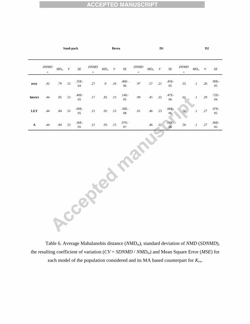
obtained for Kro are listed in Table 6. From Figures 6-9 and Tables 5 and 6 one can also observe

that model averaged results lead to high fidelity representations of the experimental observations.

MA results appear to be of higher quality than those obtained with the most skillful model (i.e.,

LET) in most cases, with particular reference to Kro. These results are consistent with the

observation that the model average can be more skillful than the model ranked as highest in cases

where the individual models in the collection lead to data interpretations of diverse qualities.

Our results generally support the findings of Kerig and Watson (1986) and Lomeland et

al. (2005) who indicated that the Corey and Chierici models are not flexible enough to reconcile

the entire set of experimental observations. However, they also suggest that in some cases, most

notably for the interpretation of Krw data, the higher complexity of the LET model does not

justify selecting it at the expenses of other, simpler models. In such scenarios, a multi-model

analysis of the kind we present can be more appropriate.

4. Conclusions

We produce high quality two-phase relative permeability datasets resulting from Steady-

State imbibition experiments on two diverse porous media, a quartz Sand-pack and a Berea

sandstone core. The ability of three commonly employed empirical two-phase models (i.e.,

Corey, Chierici and LET) to capture the observed behavior has been analyzed on the basis of

rigorous model identification criteria. The latter have been applied to rank the selected

alternative models through (a) the identification of the smallest value of a given criterion and (b)

the evaluation of weights given by posterior model probabilities, conditional on a given dataset.

We estimate the parameters of each model within a Maximum Likelihood framework for our

experiments as well as additional published datasets (Lomeland et al. 2005).

Our results show that the LET model, which relies on the largest number (three) of

uncertain parameters, appears to exhibit sufficient flexibility to satisfactorily capture the entire

set of experimental data, thus suggesting that capturing continuum scale manifestations of these

complex phenomena might require considering flexible functional forms at the expenses of a

high number of parameters. Model discrimination based on the smallest value of a given model

identification criterion reveals that KIC indicates the LET as the best model for all datasets,

while other criteria lead to contrasting results as a function of the dataset considered. A detailed

analysis of the alternative models based on posterior (conditional) probabilities reveals that in

several cases, most notably for assessment of Krw curves, the weights associated with the simple

Chierici and Corey models cannot be considered as negligible. In these cases, a single

interpretive model such as the LET which is associated with the highest number of parameters,

might not succeed in providing a complete uncertainty quantification and a multi-model analysis,

including also low-complexity models in a model averaged (MA) analysis, should be favored.

In this context, we compare the interpretative skill of the average of the model collection

to the skills of the individual members on the basis of the Normalized Mahalanobis Distance and

mean square error. Our study suggests that model averaged results tend to produce high fidelity

representations of the experimental observations, MA results being of higher quality than those

obtained with the most skillful model (i.e., LET) in most cases, with particular reference to Kro.

ACKNOLWEDGMENTS

Partial financial support from Eni SpA is gratefully acknowledged.

TABLE CAPTIONS

Table 1. Physical properties of core sample and fluids.

Table 2. Physical properties of Norwegian Continental Shelf core samples and fluids for

experiments D1 and D2 (Lomeland et al. 2005).

Table 3. Model Calibration and Identification Criteria and Corresponding Posterior Probability

(in parenthesis) associated with Krw (the smallest values for each dataset are highlighted in bold).

Table 4. Model Calibration and Identification Criteria and Corresponding Posterior Probability

(in parenthesis) associated with Kro (the smallest values for each dataset are highlighted in bold).

Table 5. Average Mahalanobis distance (NMDm), standard deviation of NMD (SDNMD), the

resulting coefficient of variation (CV = SDNMD / NMDm) and Mean Square Error (MSE) for

each model of the population considered and its MA-based counterpart for Krw.

Table 6. Average Mahalanobis distance (NMDm), standard deviation of NMD (SDNMD), the

resulting coefficient of variation (CV = SDNMD / NMDm) and Mean Square Error (MSE) for

each model of the population considered and its MA-based counterpart for Kro.

FIGURE CAPTIONS

Fig. 1. (a) Sketch of experimental set-up; (b) Steady State (SS) imbibition process.

Fig. 2. Steady-State Imbibition relative permeabilities versus average water saturation.

Fig. 3. Estimated Corey model parameter values for (a) Krw and (b) Kro associated with the four

considered datasets. Intervals associated with the upper (U) and lower (L) limits identifying the

95% uncertainty bounds around the estimate are also depicted.

Fig. 4. Estimated Chierici model parameter values for (a) Krw and (b) Kro associated with the four

considered datasets. Intervals associated with the upper (U) and lower (L) limits identifying the

95% uncertainty bounds around the estimate are also depicted.

Fig. 5. Estimated LET model parameter values for (a) Krw and (b) Kro associated with the four

considered datasets. Intervals associated with the upper (U) and lower (L) limits identifying the

95% uncertainty bounds around the estimate are also depicted.

Fig. 6. Graphical depictions of (a) Krw, (b) Kro versus water saturation for the Sand-pack

experiments together with the results of all calibrated models, uncertainty bounds corresponding

to Gaussian 95% confidence intervals and model average (MA).

Fig. 7. Graphical depictions of (a) Krw, (b) Kro versus water saturation for the Berea sandstone

experiments together with the results of all calibrated models, uncertainty bounds corresponding

to Gaussian 95% confidence intervals and model average (MA).

Fig. 8. Graphical depictions of (a) Krw, (b) Kro versus water saturation for dataset D1 together

with the results of all calibrated models, uncertainty bounds corresponding to Gaussian 95%

confidence intervals and model average (MA).

Fig. 9. Graphical depictions of (a) Krw, (b) Kro versus water saturation for dataset D2 together

with the results of all calibrated models and uncertainty bounds corresponding to Gaussian 95%

confidence intervals and model average (MA).

Ethical Statement

The authors declare that they have no conflict of interest.

References

Akaike, H., 1974. A new look at the statistical model identification. Automatic Control, IEEE

Transactions on, 19(6): 716-723.

Al-Fattah, S.M., 2003. Empirical Equations for Water/Oil Relative Permeability in Saudi Sandstone

Reservoirs. Society of Petroleum Engineers.

Botermans, C.W., van Batenburg, D.W. and Bruining, J., 2001. Relative Permeability Modifiers: Myth or

Reality? Society of Petroleum Engineers.

Cao, J., James, L.A. and Johansen, T.E., 2014. Determination of two phase relative permeability from

core floods with constant pressure boundaries. International Symposium of the Society of

CoreAnalysis ,Avignon, France, 8-1 September, 2014.

Chierici, G.L., 1984. Novel Relations for Drainage and Imbibition Relative Permeabilities.

Chierici, G.L., 1994. Principles of petroleum reservoir engineering.

Corey, A.T., 1954. The interrelation between gas and oil relative permeabilities. Prod, Monthly

Craig, F.F., 1993. The reservoir engineering aspects of waterflooding. Richardson, TX: Henry L. Doherty

Memorial Fund of AIME, Society of Petroleum Engineers.

Ebeltoft, E., Lomeland, F., Brautaset, A. and Haugen, Å., 2014. Parameter based scal-analysing relative

permeability for full field application. International Symposium of the Society of Core

Analysis,Avignon, France, 8-11 September, 2014.

Ebeltoft, F.L.E., 2014. Versatile three-phase correlations for relative permeability and capillary pressure.

Feigl, A., 2011. Treatment of relative permeabilities for application in hydrocarbon reservoir simulation

model. Nafta, 62(7-8): 233-243.

Firoozabadi, A. and Aziz, K., 1991. Relative Permeabilities From Centrifuge Data.

Honarpour, M., Koederitz, L. and Harvey, A.H., 1986. Relative permeability of petroleum reservoirs.

C.R.C. Press.

Honarpour, M., Koederitz, L.F. and Harvey, A.H., 1982. Empirical Equations for Estimating Two-Phase

Relative Permeability in Consolidated Rock.

Hurvich, C.M. and Tsai, C.-L., 1989. Regression and time series model selection in small samples.

Biometrika, 76(2): 297-307.

Kashyap, R.L., 1982. Optimal Choice of AR and MA Parts in Autoregressive Moving Average Models.

IEEE Transactions on Pattern Analysis and Machine Intelligence, PAMI-4(2): 99-104.

Kikuchi, M.M., Branco, C.C., Bonet, E.J., Zanoni, R.M. and Paiva, C.M., 2005. Water Oil Relative

Permeability Comparative Study: Steady Versus UnSteady State.

Kjosavik, A., Ringen, J.K. and Skjaeveland, S.M., 2002. Relative Permeability Correlation for Mixed-

Wet Reservoirs.

Lake, L.W., 1986. Fundamentals of enhanced oil recovery. Society of Petroleum Engineers.

Liu, R., Liu, H., Li, X., Wang, J. and Pang, C., 2010. Calculation of Oil and Water Relative Permeability

for Extra Low Permeability Reservoir. Society of Petroleum Engineers.

Lomeland, F., Ebeltoft, E. and Thomas, W.H., 2005. A new versatile relative permeability correlation,

International Symposium of the Society of Core Analysts, Toronto, Canada, pp. 21-25.

Lu, D., 2012. Assessment Of Parametric And Model Uncertainty In Groundwater Modeling, Electronic

Thesis, Treatises and sissertations, Paper 5003, http://diginole.lib.fsu.edu/etd/5003.

Lu, D., Ye, M. and Neuman, S., 2011. Dependence of Bayesian Model Selection Criteria and Fisher

Information Matrix on Sample Size. Math Geosci, 43(8): 971-993.

Mian, M.A., 1992. Petroleum Engineering Handbook for the Practicing Engineer. PennWell Books.

Schwarz, G., 1978. Estimating the dimension of a model. The annals of statistics, 6(2): 461-464.

Sendra, 2013. User guide.

Sigmund, P. and McCaffery, F., 1979. An improved unsteady-state procedure for determining the

relative-permeability characteristics of heterogeneous porous media (includes associated papers

8028 and 8777). Society of Petroleum Engineers Journal, 19(01): 15-28.

Silpngarmlers, N., Guler, B., Ertekin, T. and Grader, A.S., 2002. Development and Testing of Two-Phase

Relative Permeability Predictors Using Artificial Neural Networks.

Slider, H.C., 1983. Worldwide Practical Petroleum Reservoir Engineering Methods. PennWell Books.

Sylte, A., Ebeltoft, E. and Petersen, E.B., 2004. Simultaneous Determination of Relative Permeability and

Capillary Pressure Using Data from Several Experiments.

Toth, J., Bodi, T., Szucs, P. and Civan, F., 2002. Convenient formulae for determination of relative

permeability from unsteady-state fluid displacements in core plugs. Journal of Petroleum Science

and Engineering, 36(1–2): 33-44.

Ye, M., Meyer, P.D. and Neuman, S.P., 2008. On model selection criteria in multimodel analysis. Water

Resources Research, 44(3).

Ye, M., Pohlmann, K.F., Chapman, J.B., Pohll, G.M. and Reeves, D.M., 2010. A model‐averaging

method for assessing groundwater conceptual model uncertainty. Groundwater, 48(5): 716-728.

Table A1. Steady-State Imbibition Relative Permeabilities (Krw: oil relative permeability;

Kro: water relative permeability) and water saturation, Sw, for the sand-pack and the Berea

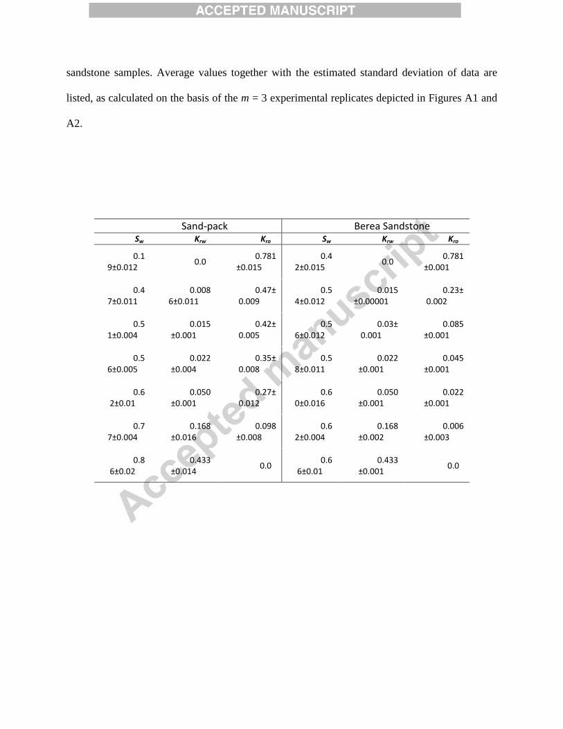
sandstone samples. Average values together with the estimated standard deviation of data are

listed, as calculated on the basis of the m = 3 experimental replicates depicted in Figures A1 and

A2.

Sand-pack Berea Sandstone Sw Krw Kro Sw Krw Kro

0.19±0.012

0.0 0.781

±0.015 0.4

2±0.015 0.0

0.781±0.001

0.47±0.011

0.0086±0.011

0.47±0.009

0.54±0.012

0.015±0.00001

0.23±0.002

0.51±0.004

0.015±0.001

0.42±0.005

0.56±0.012

0.03±0.001

0.085±0.001

0.56±0.005

0.022±0.004

0.35±0.008

0.58±0.011

0.022±0.001

0.045±0.001

0.62±0.01

0.050±0.001

0.27±0.012

0.60±0.016

0.050±0.001

0.022±0.001

0.77±0.004

0.168±0.016

0.098±0.008

0.62±0.004

0.168±0.002

0.006±0.003

0.86±0.02

0.433±0.014

0.0 0.6

6±0.01 0.433

±0.001 0.0

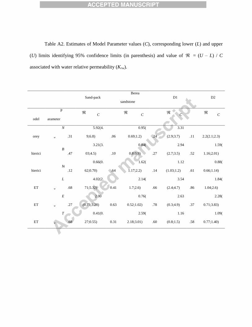
Table A2. Estimates of Model Parameter values (C), corresponding lower (L) and upper

(U) limits identifying 95% confidence limits (in parenthesis) and value of = (U – L) / C

associated with water relative permeability (Krw).

Sand-pack

Berea

sandstone

D1 D2

M

odel

P

arameter

C

C

C

C

C

orey

N

w

0

.31

5.92(4.

9;6.8)

0

.06

0.95(

0.69;1.2)

0

.24

3.31

(2.9;3.7)

0

.11

2.2(2.1;2.3)

C

hierici

B

0

.47

3.21(3.

03;4.5)

0

.10

0.84(

0.8;0.9)

0

.27

2.94

(2.7;3.5)

0

.52

1.59(

1.16;2.01)

C

hierici

M

0

.12

0.66(0.

62;0.70)

0

.64

1.62(

1.17;2.2)

0

.14

1.12

(1.03;1.2)

0

.61

0.88(

0.66;1.14)

L

ET

L

w

0

.68

4.02(2.

71;5.32)

0.41

2.14(

1.7;2.6)

0

.66

3.54

(2.4;4.7)

0

.86

1.84(

1.04;2.6)

L

ET

E

w

1

.27

2.00

(0.73;3.28)

0.63

0.76(

0.52;1.02)

1

.78

2.63

(0.3;4.9)

1

.37

2.28(

0.71;3.83)

L

ET

T

w

0

.68

0.41(0.

27;0.55)

0.31

2.59(

2.18;3.01)

0

.60

1.16

(0.8;1.5)

0

.58

1.09(

0.77;1.40)

Table A3. Estimates of Model Parameter values (C), corresponding lower (L) and upper

(U) limits identifying 95% confidence limits (in parenthesis) and value of = (U – L) / C

associated with oil relative permeability (Kro).

Sand-pack

Berea

sandstone

D1 D2

M

odel

P

arameter

C

C

C

C

C

orey

N

o

0

.06

1.02(

0.99;1.05)

0

.36

2.18(

1.8;2.6)

0

.37

2.05(

1.67;2.43)

0

.04

3.95(

3.86;4.40)

C

hierici

A

0

.16

0.67(

0.62;0.73)

0

.26

1.27(

1.11;1.44)

0

.10

1.54(

1.46;1.62)

0.07

2.90(

2.78;3.01)

C

hierici

L

0

.36

0.64(

0.53;0.76)

0

.68

1.35(

0.89;1.81)

0

.17

1.40(

1.28;1.52)

0.05

0.89(

0.88;0.92)

L

ET

L

o

0

.43

1.00(

0.79;1.22)

0

.41

3.31(

3.08;3.54)

0

.39

3.11(

2.5;3.72)

0

.09

4.28(

4.08;4.49)

L

ET

E

o

0

.80

1.18(

0.70;1.65)

0

.63

1.36(

1.14;1.59)

1

.40

1.60(

0.48;2.74)

0

.29

1.36(

1.15;1.56)

L

ET

T

o

0

.57

1.28(

0.91;1.64)

1

.51

2.39(

0.58;4.29)

0

.42

1.83(

1.45;2.22)

0

.15

0.66(

0.61;0.71)

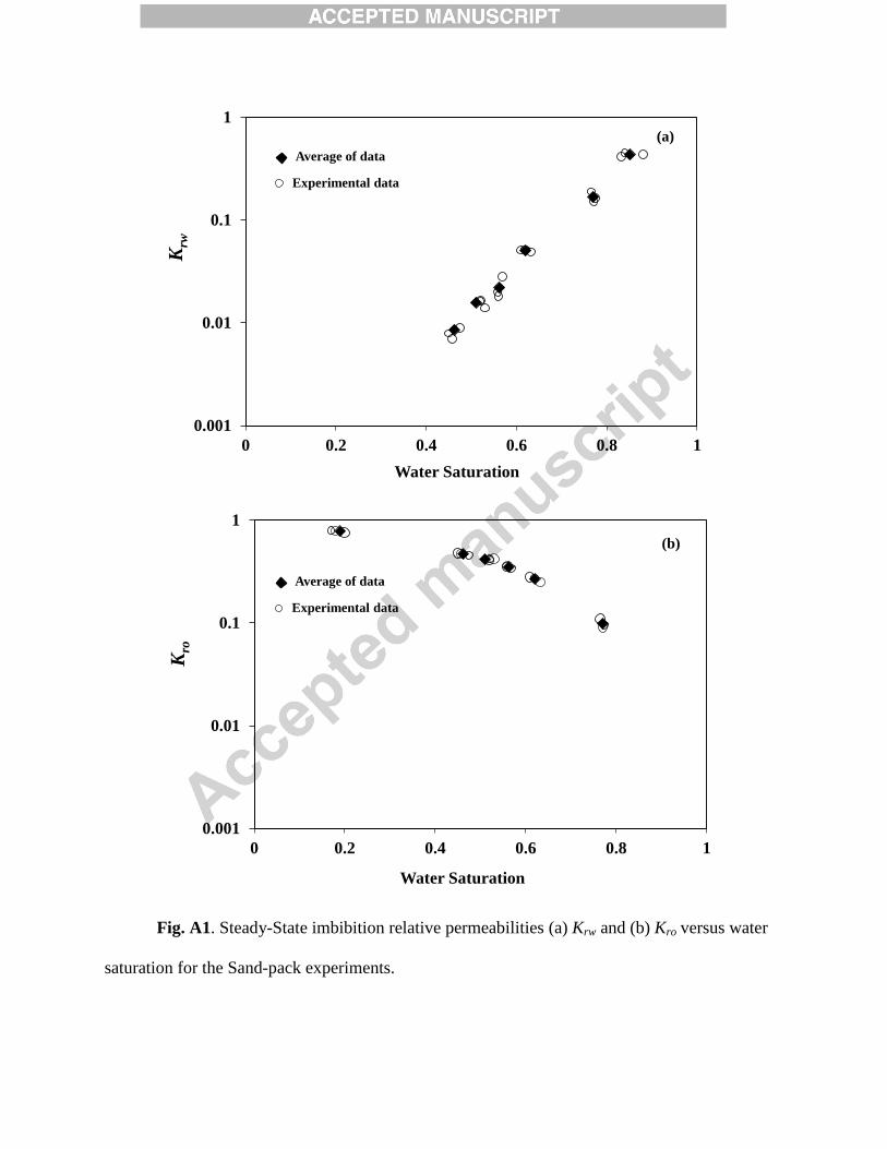
Fig. A1. Steady-State imbibition relative permeabilities (a) Krw and (b) Kro versus water

saturation for the Sand-pack experiments.

0.001

0.01

0.1

1

0 0.2 0.4 0.6 0.8 1

0.001

0.01

0.1

1

0 0.2 0.4 0.6 0.8 1

Water Saturation

Krw

(a)

Water Saturation

Kro

(b)

Average of data

Experimental data

Average of data

Experimental data

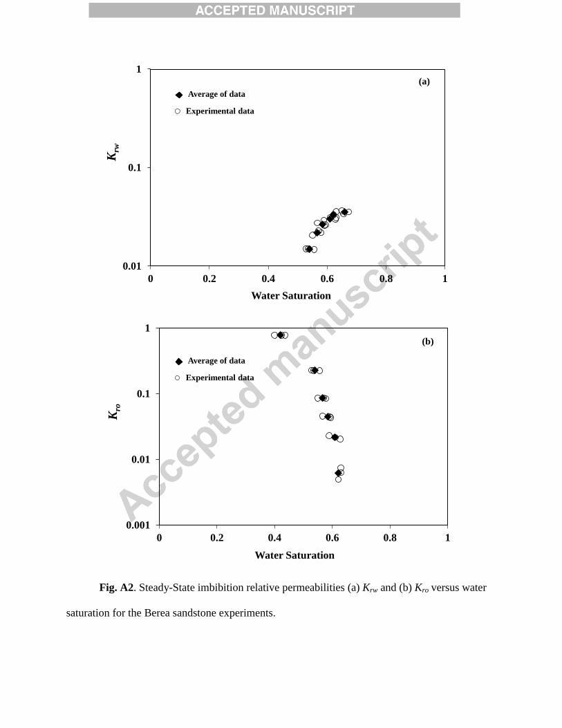
Fig. A2. Steady-State imbibition relative permeabilities (a) Krw and (b) Kro versus water

saturation for the Berea sandstone experiments.

0.001

0.01

0.1

1

0 0.2 0.4 0.6 0.8 1

0.01

0.1

1

0 0.2 0.4 0.6 0.8 1

Water Saturation

Krw

(a)

Water Saturation

Kro

(b)

Average of data

Experimental data

Average of data

Experimental data

Fig. A3. Posterior probabilities associated with the models tested based on KIC and on

Krw data interpretation.

0

0.2

0.4

0.6

0.8

1

Corey Cherici LET0

0.2

0.4

0.6

0.8

1

Corey Cherici LET

0

0.2

0.4

0.6

0.8

1

Corey Cherici LET0

0.2

0.4

0.6

0.8

1

Corey Cherici LET

Po

ster

ior

pro

ba

bil

ity

Po

ster

ior

pro

ba

bil

ity

Po

ster

ior

pro

ba

bil

ity

Po

ster

ior

pro

ba

bil

ity

Sand-pack Berea Sandstone

Dataset D1 Dataset D2

Fig. A4. Posterior probabilities associated with the models tested based on KIC and on

Kro data interpretation.

0

0.2

0.4

0.6

0.8

1

Corey Cherici LET0

0.2

0.4

0.6

0.8

1

Corey Cherici LET

0

0.2

0.4

0.6

0.8

1

Corey Cherici LET

0

0.2

0.4

0.6

0.8

1

Corey Cherici LET

Po

ster

ior

pro

ba

bil

ity

Post

erio

r p

rob

ab

ilit

y

Po

ster

ior

pro

ba

bil

ity

Po

ster

ior

pro

ba

bil

ity

Sand-pack Berea Sandstone

Dataset D1 Dataset D2

Fig. 1. (a) Sketch of experimental set-up; (b) Steady State (SS) imbibition process.

100 % Water

100 % Oil

Absolute Water Permeability

Measured (Kw)

100 % Water

Oil Permeability Measured at

(Swi)

Oil

Water

Oil

Water

Oil

Water

Oil

WaterSor

Joint Injection of Oil and

Water Fractional flow

Swi

Imb

ibit

ion

X-RAY

Outlet

Pressure

Inlet

Pressure

Oil Pump

Water Pump

Confining

Pressure Oil

Water

Calibration

Blocks

X-RAY Detector

a b

Step A

Step C

Step B

Step E

Step D

Step F

Permeability Measured at

(Sor)

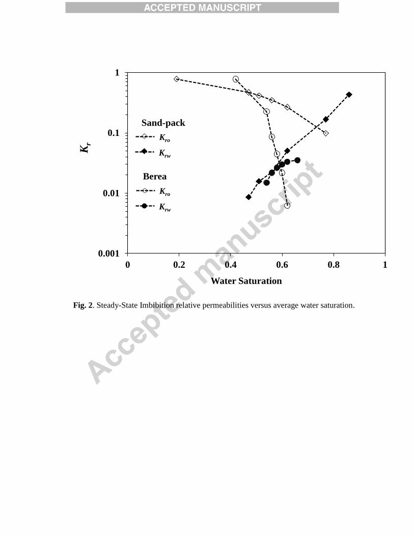
Fig. 2. Steady-State Imbibition relative permeabilities versus average water saturation.

0.001

0.01

0.1

1

0 0.2 0.4 0.6 0.8 1

Water Saturation

Kr

Kro

Krw

Berea

Kro

Krw

Sand-pack

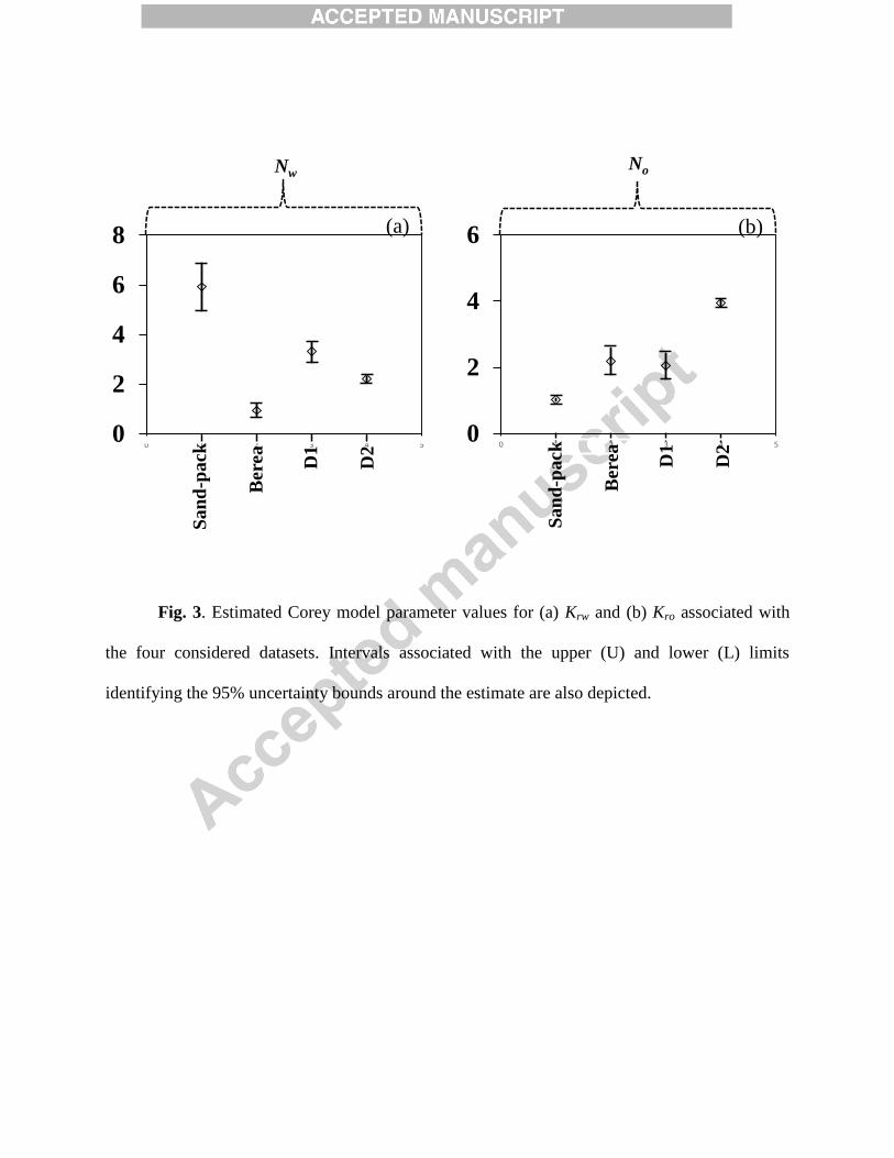
Fig. 3. Estimated Corey model parameter values for (a) Krw and (b) Kro associated with

the four considered datasets. Intervals associated with the upper (U) and lower (L) limits

identifying the 95% uncertainty bounds around the estimate are also depicted.

0

2

4

6

8

0 1 2 3 4 50

2

4

6

0 1 2 3 4 5

NwNo

(a) (b)

San

d-p

ack D1

D2

Ber

ea

Sa

nd

-pa

ck D1

D2

Ber

ea

Fig. 4. Estimated Chierici model parameter values for (a) Krw and (b) Kro associated with

the four considered datasets. Intervals associated with the upper (U) and lower (L) limits

identifying the 95% uncertainty bounds around the estimate are also depicted.

0

1

2

3

4

0 2 4 6 8 10 12 14 16 18 20 0

1

2

3

4

0 2 4 6 8 10 12 14 16 18 20

(a)S

an

d-p

ack D

1

D2

Ber

ea

Sa

nd

-pa

ck D1

D2

Ber

ea

(b)

San

d-p

ack D1

D2

Ber

ea

Sa

nd

-pa

ck D1

D2

Ber

ea

B M A L

Fig. 5. Estimated LET model parameter values for (a) Krw and (b) Kro associated with the

four considered datasets. Intervals associated with the upper (U) and lower (L) limits identifying

the 95% uncertainty bounds around the estimate are also depicted.

0

1

2

3

4

5

6

0 4 8 12 16 20 24 28 32 36 40 44 48 52 56 600

1

2

3

4

5

0 4 8 12 16 20 24 28 32 36 40 44 48 52 56 60

(a)S

an

d-p

ack D

1D

2

Ber

ea

Sa

nd

-pa

ck D1

D2

Ber

ea

Sa

nd

-pa

ck D1

D2

Ber

ea

LwEw Tw

(b)

Sa

nd

-pa

ck D1

D2

Ber

ea

Sa

nd

-pa

ck D1

D2

Ber

ea

Sa

nd

-pa

ck D1

D2

Ber

ea

LoEo To

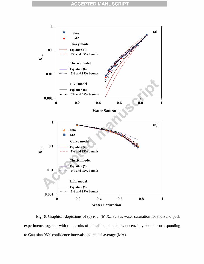
Fig. 6. Graphical depictions of (a) Krw, (b) Kro versus water saturation for the Sand-pack

experiments together with the results of all calibrated models, uncertainty bounds corresponding

to Gaussian 95% confidence intervals and model average (MA).

0.001

0.01

0.1

1

0 0.2 0.4 0.6 0.8 1

0.001

0.01

0.1

1

0 0.2 0.4 0.6 0.8 1

data

Water Saturation

Krw

(a)

Water Saturation

Kro

(b)

data

5% and 95% bounds

Equation (8)

LET model

5% and 95% bounds

Equation (6)

Cherici model

5% and 95% bounds

Equation (3)

Corey model

5% and 95% bounds

Equation (9)

LET model

5% and 95% bounds

Equation (7)

Cherici model

5% and 95% bounds

Equation (4)

Corey model

MA

MA

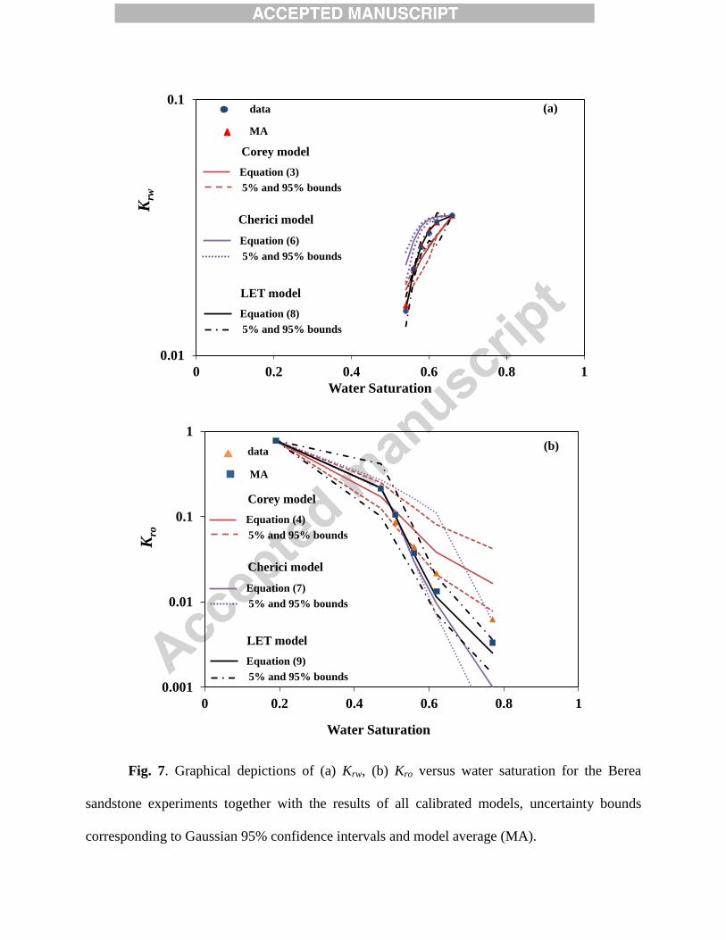
Fig. 7. Graphical depictions of (a) Krw, (b) Kro versus water saturation for the Berea

sandstone experiments together with the results of all calibrated models, uncertainty bounds

corresponding to Gaussian 95% confidence intervals and model average (MA).

0.01

0.1

0 0.2 0.4 0.6 0.8 1

0.001

0.01

0.1

1

0 0.2 0.4 0.6 0.8 1

Water Saturation

Krw

(a)

Water Saturation

Kro

(b)

MA

5% and 95% bounds

Equation (8)

LET model

5% and 95% bounds

Equation (6)

Cherici model

5% and 95% bounds

Equation (3)

Corey model

5% and 95% bounds

Equation (9)

LET model

5% and 95% bounds

Equation (7)

Cherici model

5% and 95% bounds

Equation (4)

Corey model

data

data

MA

Fig. 8. Graphical depictions of (a) Krw, (b) Kro versus water saturation for dataset D1

together with the results of all calibrated models, uncertainty bounds corresponding to Gaussian

95% confidence intervals and model average (MA).

0.001

0.01

0.1

1

0 0.2 0.4 0.6 0.8 1

0.001

0.01

0.1

1

0 0.2 0.4 0.6 0.8 1

Water Saturation

Krw

(a)

Water Saturation

Kro

(b)

data

5% and 95% bounds

Equation (8)

LET model

5% and 95% bounds

Equation (6)

Cherici model

5% and 95% bounds

Equation (3)

Corey model

5% and 95% bounds

Equation (9)

LET model

5% and 95% bounds

Equation (7)

Cherici model

5% and 95% bounds

Equation (4)

Corey model

data

MA

MA

Fig. 9. Graphical depictions of (a) Krw, (b) Kro versus water saturation for dataset D2

together with the results of all calibrated models and uncertainty bounds corresponding to

Gaussian 95% confidence intervals and model average (MA).

0.001

0.01

0.1

1

0 0.2 0.4 0.6 0.8 1

0.001

0.01

0.1

1

0 0.2 0.4 0.6 0.8 1

Water Saturation

Krw

(a)

Water Saturation

Kro

(b)

5% and 95% bounds

Equation (8)

data

5% and 95% bounds

Equation (6)

Cherici model

5% and 95% bounds

Equation (3)

Corey model

5% and 95% bounds

Equation (9)

LET model

5% and 95% bounds

Equation (7)

Cherici model

5% and 95% bounds

Equation (4)

Corey model

LET model

data

MA

MA

Highlights:

We perform high quality steady-state two-phase relative permeability

measurements.

We illustrate the formal model identification criteria to rank and evaluate a set of

alternative models.

We compare the performance of a model averaging approach with skill of each

individual model.

Comparison have been carried out on the basis of the Normalized Mahalanobis

Distance and mean square error.

The results show that model averaged tend to produce high fidelity

representations of the observations.

Table 1. Physical properties of the tested core samples and fluids.

Sand

-pack

Bere

a

Oil viscosity [cP] 1.74 1.74

Water viscosity [cP] 0.97 1.03

Temperature during test [C] 25 25

Porosity [%] 37 17

Water absolute permeability [mD]

Permeability of oil at Swi [mD]

2900

2500

30

25

Table 2. Physical properties of Norwegian Continental Shelf core samples and fluids for

experiments D1 and D2 (Lomeland et al. 2005)).

D1 D2

Oil viscosity [cP] 2.41 0.67

Water viscosity [cP]

0.39

5

0.30

6

Temperature for test [C] 84 95

Porosity [%] 29 27

Swi [-]

Permeability of oil at Swi [mD]

0.19

6

2396

0.07

9

1042

Table 3. Model Calibration and Identification Criteria and Corresponding Posterior

Probability (in parenthesis) associated with Krw (the smallest values for each dataset are

highlighted in bold).

Su

bsets

AIC AICc BIC KIC

C

orey

Sa

nd-pack

-59(0.02)

-56.24(0.04)

-

59.39(0.02)

-

62.99(0.05)

Be

rea

-67(0.017) -62.83(0.14)

-

67.24(0.02)

-

67.96(0.025)

D

1

-96(0.014) -94.23(0.027)

-

95.34(0.015)

-

98.23(0.024)

D

2

-64(0.37) -61.37(0.83)

-

64.48(0.39)

-

60.9(0.30)

C

hierici

Sa

nd-pack

-79(0.54)

-71.60(0.84)

-

79.76(0.55)

-

73.76(0.31)

Be

rea

-75(0.06) -67.01(0.29)

-

75.17(0.06)

-

81.04(0.58)

D

1

-117(0.49) -113.12(0.64) -

116.2(0.50)

-

113.98(0.33)

D

2

-57(0.012) -49.02(0.11)

-

57.18(0.12)

-

56.69(0.15)

L

ET

Sa

nd-pack

-78(0.44)

-58.49 (0.09)

-

78.74(0.47)

-

76.18(0.64)

Be

rea

-91(0.92) -71.04(0.56) -

91.25(0.92)

-

89.48(0.92)

D

1

-117.3(0.5) -109.3(0.33)

-

116.06(0.49)

-

118.02(0.65)

D

2

-66(0.51) -45.67(0.061) -

65.9(0.49)

-

64.31(0.54)

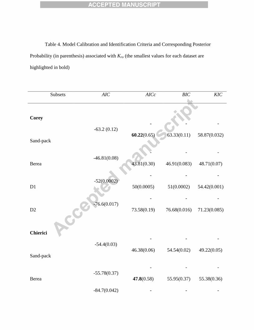
Table 4. Model Calibration and Identification Criteria and Corresponding Posterior

Probability (in parenthesis) associated with Kro (the smallest values for each dataset are

highlighted in bold)

Subsets AIC AICc BIC KIC

Corey

Sand-pack

-63.2 (0.12)

-

60.22(0.65)

-

63.33(0.11)

-

58.87(0.032)

Berea

-46.81(0.08)

-

43.81(0.30)

-

46.91(0.083)

-

48.71(0.07)

D1

-52(0.0002)

-

50(0.0005)

-

51(0.0002)

-

54.42(0.001)

D2

-76.6(0.017)

-

73.58(0.19)

-

76.68(0.016)

-

71.23(0.085)

Chierici

Sand-pack

-54.4(0.03)

-

46.38(0.06)

-

54.54(0.02)

-

49.22(0.05)

Berea

-55.78(0.37) -

47.8(0.58)

-

55.95(0.37)

-

55.38(0.36)

-84.7(0.042) - - -

Table 5. Average Mahalanobis distance (NMDm), standard deviation of NMD (SDNMD),

the resulting coefficient of variation (CV = SDNMD / NMDm) and Mean Square Error (MSE) for

each model of the population considered and its MA based counterpart for Krw.

D1 80(0.0789) 83.78(0.043) 80.82(0.08)

D2

-79(0.025) -

71.6(0.14)

-

79.8(0.03)

-

71.85(0.10)

LET

Sand-pack

-75.1(0.85)

-

55.08(0.28)

-

75.29(0.85)

-

66.67(0.92)

Berea

-57.97(0.54) -

37.97(0.11)

-

58.18(0.54)

-

58.72(0.57)

D1 -103.5(0.96) -

95.53(0.92)

-

102.32(0.96)

-

98.74(0.92)

D2 -101(0.96) -

81.03(0.68)

-

101.25(0.96)

-

84.57(0.82)

Sand-pack Berea D1 D2

S

DNMD

m

N

MDm

C

V

M

SE

S

DNMD

m

N

MDm

C

V

M

SE

S

DNMD

m

N

MDm

C

V

M

SE

S

DNMD

m

N

MDm

C

V

M

SE

C

orey

1

.42

2

.79

0

.51

8

.35E-

04

1

.27

8

.9

0

.16

6

.40E-

06

0

.97

4

.57

0

.21

4

.45E-

05

0

.55

2

.1

0

.26

7

.90E-

05

C

hierici

1

.44

2

.85

0

.51

3

.40E-

05

1

.17

7

.82

0

.15

2

.14E-

05

0

.99

4

.45

0

.22

4

.47E-

06

0

.61

2

.1

0

.29

1

.72E-

04

LET

1

.44

2

.84

0

.51

3

.00E-

05

1

.21

7

.92

0

.15

8

.30E-

08

1

.01

4

.46

0

.23

3

.06E-

06

0

.56

2

.1

0

.27

3

.07E-

05

M

A

1

.44

2

.84

0

.51

3

.36E-

05

1

.21

7

.93

0

.15

2

.07E-

07

1 4

.46

0

.22

3

.06E-

06

0

.56

2

.1

0

.27

5

.06E-

05

Table 6. Average Mahalanobis distance (NMDm), standard deviation of NMD (SDNMD),

the resulting coefficient of variation (CV = SDNMD / NMDm) and Mean Square Error (MSE) for

each model of the population considered and its MA based counterpart for Kro.

Sand-pack Berea D1 D2

S

DNMD

m

N

MDm

C

V

M

SE

S

DNMD

m

N

MDm

C

V

M

SE

S

DNMD

m

N

MDm

C

V

M

SE

S

DNMD

m

N

MDm

C

V

M

SE

C

orey

1

.04

1

.84

0

.56

4

.80E-

04

1

.74

1

.71

1

.01

7

.04E-

04

1

.65

1

.42

1

.11

3

.60E-

03

0

.99

0

.88

1

.13

9

.00E-

06

C

hierici

1

.04

1

.86

0

.56

0

.0013

1

.72

1

.66

1

.03

1

.14E-

04

1

.59

1

.32

1

.21

1

.15E-

04

0

.99

0

.87

1

.14

4

.90E-

06

L

ET

1

.03 2

0

.51

4

.90E-

05

1

.71

1

.65

1

.02

8

.10E-

05

1

.58

1

.31

1

.21

2

.32E-

05

0

.99

0

.87

1

.14

1

.72E-

07

M

A

1

.03 2

0

.51

6

.80E-

05

1

.72

1

.67

1

.02

9

.37E-

05

1

.59

1

.32

1

.21

2

.04E-

05

0

.99

0

.87

1

.14

1

.06E-

08