author's personal copy - oregon state...

Author's personal copy

In-stand scenic beauty of variable retention harvests and mature forestsin the U.S. Pacific Northwest: The effects of basal area, density,retention pattern and down wood

Robert G. Ribe*

Institute for a Sustainable Environment and Department of Landscape Architecture, 5234 University of Oregon, Eugene, OR 97403, USA

a r t i c l e i n f o

Article history:Received 31 December 2008Received in revised form28 July 2009Accepted 25 August 2009Available online 23 September 2009

Keywords:Forest aestheticsEcological forestryNew forestryVariable retentionScenic standardsPacific NorthwestForest structureDown woodWoody debris

a b s t r a c t

Tensions between amenity- and timber-based economies in the U.S. and Canadian Pacific Northwestmotivated a study of scenic beauty inside mature forests and timber harvests. A diverse sample ofregional forests, measures of forest structure, and large, representative samples of photographs andpublic judges were employed to measure scenic beauty inside un-harvested mature and old-growthforests, and timber harvests. The latter varied systematically in down wood levels and retention level andpattern. Scenic beauty tended to be optimized at a basal area of 110–155 m3/ha and/or 700–900 trees/ha.Older forests and those with larger trees were perceived to be more beautiful. In harvests, greaterretention levels, less down wood, and dispersed rather than aggregated retention patterns contributed toaesthetic improvements. Green-tree retention harvests offer considerable potential gains in perceivedscenic beauty compared to perceived very ugly clearcuts, particularly at higher retention levels. Thesegains are more reliable from dispersed retention patterns. The silvicultural parameters studied changestrength in affecting scenic beauty with changes in retention level. These interactions are explored inrelation to a range of scenic quality objectives as an aid to planners, visual impact analysts, andsilviculturists.

� 2009 Elsevier Ltd. All rights reserved.

1. Introduction

Scenic beauty is an important issue affecting socially acceptableforestry and timber harvest decisions (Sheppard et al., 2001; Bliss,2000). There is an extensive literature about this problem,summarized by Ribe (1989), Rosenberger and Smith (1998), andRyan (2005), and aesthetic values are regularly considered in forestplanning decisions. Some public agencies systematically accountfor scenic impacts in forest landscapes and timber harvests (USDAForest Service, 1995; British Columbia Ministry of Forests, 2001),and forest plan optimizations can include measures of scenicproduction (e.g. Alho and Kangas, 1997; Leskinen et al., 2006).

Managing the aesthetics of timber harvests is salient in the U.S.Pacific Northwest and western Canada (Shindler et al., 2002;Sheppard, 2003). Many immigrants and visitors to this region havestrong expectations of a high quality of life, scenic amenities, anda non-exploitive relationship with nature (Niemi and Whitelaw,1999; Durning, 1999). These newcomers often value ecology inforest management (Ribe and Matteson, 2002) and many value

perceptions of a naturally healthy regional environment, whetheror not they directly use it for recreation or livelihood (Niemi andWhitelaw, 1999). The region’s population tends to use simple,affective perceptions of scenic beauty as a cue to landscapes’acceptable management (Ribe, 2002). Scenic beauty also influencescognitive judgments of timber harvests’ acceptability, along withinformation about wildlife impacts, the intensity of harvests, andeconomic benefits (Ribe, 2006).

The regional conflict between these popular, naturalisticexpectations of forests versus traditional, intensive silviculturecame to a head in the U.S. via the spotted owl controversy of the late1980s and early 1990s (Dietrich, 1992; Yaffee, 1994). This conflictproved socially traumatic and very contentious (Carroll, 1995;Durbin, 1996), and produced the Northwest Forest Plan (NFP)(USDA and USDI, 1994). This highly prescriptive plan has substan-tially modified planning and silvicultural practices in public foreststhroughout major portions of three U.S. states. The NFP seeks toapply ecosystem management principles (e.g. Bormann et al., 1994).These promote ‘‘New Forestry’’ ideas, as opposed to plantation orclearcut-based forestry (Debell and Curtis, 1993; Swanson andFranklin, 1992). The NFP requires variable retention timber harvests(Franklin et al., 1997), which are also gaining favor in western

* Corresponding author. Tel.: þ01 541 346 3648; fax: þ01 541 346 3626.E-mail address: [email protected]

Contents lists available at ScienceDirect

Journal of Environmental Management

journal homepage: www.elsevier .com/locate/ jenvman

0301-4797/$ – see front matter � 2009 Elsevier Ltd. All rights reserved.doi:10.1016/j.jenvman.2009.08.014

Journal of Environmental Management 91 (2009) 245–260


Canada in response to growing ecological and aesthetic publicconcerns (Cashore et al., 2000).

New Forestry principally aims to reduce the ecological impact oftimber harvests to better sustain soil, hydrologic, habitat, and plantcommunity functions (Franklin et al., 1989). A major technique isretention of green trees, which may also reduce the ‘‘aesthetic dip’’associated with harvests (Sheppard et al., 2001; Silvennoinen et al.,2002). This is possible in vista views (Ribe, 2005a; Karjalainen andKomulainen, 1999; British Columbia Ministry of Forests, 1997;Palmer, 2008), and is arguably an ethical intention of New Forestry(McQuillan, 1993).

Forests are also extensively experienced from within, as peopletravel through, recreate and work in them. In-stand forest sceneryis therefore also important, and often a point of affective contentionin forest management debates (e.g. DeVall, 1994), and the extent ofNew Forestry’s scenic benefits inside forests are problematic.Adverse visual impacts from retention harvests may occur due tohigh prescribed levels of down wood and snags, too few retainedtrees, or extensive clearcut areas within harvests (Gobster, 1996,1999; Sheppard, 2003), or a general appearance of lack of care forthe forest (Nassauer, 1995; Sheppard, 2001). Such adverse aestheticaffects inside variable retention harvests have received littlesystematic investigation.

This study focused on in-stand views of the most contendedforests in the controversies outlined above, namely mature forests,timber harvests within these, and old-growth forests. The goal wasto better understand, assess and manage the visual impact oftransitions among these. Do readily measurable forest and harvestattributes usefully relate to perceived scenic beauty inside forests inthe Pacific Northwest? This study sought to model in-stand forestaesthetics to establish regionally useful prescriptive parameters. Tothis end it employed unusually extensive and diverse samples offorests, forest scenes, and public judges. It employed only commonmeasures of forests’ and timber harvests’ structure to predictperceived scenic beauty.

2. Background

2.1. Review of in-stand forest scenery findings

A few studies have explored aesthetic perceptions of green-treeretention harvests. Tonnes et al. (2004) used visual simulations tostudy low levels of retention. They found that a basal area of 3 m2/ha was a threshold where average ratings began to rise above thosefor clearcuts, and scenic beauty increased with more retention fromthere. They found dispersed retention patterns more scenicallypositive than aggregated patterns, that larger retained trees andtrees in better-looking condition also helped, and that retainedundergrowth of shrubs and saplings in clearcuts slightly improvedscenic perceptions. British Columbia Ministry of Forests (1997)systematically investigated relationships between percent green-tree retention and public scenic quality perceptions, along withexpert judgments of achieved visual quality goals. They found that50% or more retention will most probably achieve high scenic‘‘retention’’ standards, 30–50% (sometimes 20%) will probablyachieve moderate ‘‘partial retention’’ standards, and 0–20% willtypically achieve low ‘‘modification’’ scenic standards. They foundthat dispersed retention patterns are perceived as more acceptablethan aggregated patterns, with the latter perceived about equally asclearcuts. Ford et al. (2009), Ribe (2006), and British ColumbiaMinistry of Forests (2006) studied acceptability perceptions ofvariable retention harvests but do not report any findings regardingaesthetic perceptions.

Studies exploring scenic perceptions of traditional silviculturaltreatments allow inferences about variable retention harvests.

Thinnings can produce moderate to high scenic beauty (Silven-noinen et al., 2002; Bradley et al., 2004; Brunson and Shelby, 1992).The size of clearcut ‘‘rooms’’ in in-stand views can matter (Tveit,2009). Small group selection cuts are scenically preferred toharvests entailing large openings (Bradley et al., 2004; Lindhagen,1996; Karjalainen, 1996). Shelterwood, seed tree and two-ageretention harvests garner similar or better average ratings asselection cuts, depending upon retention density (Bradley et al.,2004; Brunson and Shelby, 1992). Patch cuts producing large,clearcut openings do not generally garner favorable scenicperceptions (Bradley et al., 2004; Brunson and Shelby, 1992;Karjalainen, 1996; Brown and Daniel, 1986; Schweitzer et al., 1976;Echelberger, 1979), but may be scenically better over time (Brush,1976; Arthur, 1977; Shelby et al., 2003). These findings suggest thatNew Forestry harvests have much aesthetic potential compared toclearcuts and plantations, but much may depend upon evidence ofharvesting ‘‘violence’’ (Chokor and Mene, 1992; Echelberger, 1979;Benson and Ullrich, 1981; Liao and Nogami, 1999).

Because New Forestry harvests can leave a moderate number ofstanding trees, and more than most traditional harvests, theyshould be more scenically successful, because both very-high andvery-low stand densities tend to produce low scenic beautyperceptions (Silvennoinen et al., 2001; Ribe, 1990; Rudis et al.,1988;Hull et al., 1987; Vodak et al., 1985; Buhyoff et al., 1986; McCool andBenson, 1988; Kaplan and Kaplan, 1989; Schroeder and Daniel,1981; Daniel and Boster, 1976; Schweitzer et al., 1976; Kim andWells, 2005). Retaining more of the largest, most commerciallyvaluable trees also adds aesthetic value (Bradley et al., 2004;Silvennoinen et al., 2001; Rudis et al., 1988; Brown and Daniel,1986; Ribe, 1990; Hull and Buhyoff, 1986; Schroeder and Daniel,1981; Arthur, 1977; Daniel and Boster, 1976; Pukkala et al., 1988).

The retention of down wood as habitat (Harmon et al., 1986), orfor soil maintenance (Stark,1988) is more aesthetically problematic.It will tend to reduce perceived scenic beauty (Schroeder and Daniel,1981; Vodak et al., 1985; Brown and Daniel, 1986; Ribe, 1990;Schweitzer et al., 1976; Daniel and Boster, 1976; Arthur, 1977). Snagretention or creation in harvests may be problematic in affectingscenic beauty perceptions (Tonnes et al., 2004; Brunson and Shelby,1992; Brush, 1979) but can add favorably to informed acceptabilityperceptions (Brunson and Shelby, 1992; Shelby et al., 2003).

2.2. Harvest design and visual impact assessment and planning

In response to mandates to account for and mitigate visuallandscape impacts, the U.S. Forest Service and British ColumbiaMinistry of Forests have employed and updated visual resourcemanagement (VRM) systems (USDA Forest Service, 1995; BritishColumbia Ministry of Forests, 2001). Among other things, thesesystems apply scenic standards to harvest designs, which vary byforests’ visibility, natural scenic quality, visitation numbers, scenicsensitivity of viewers’ activities and forests’ importance to publicconstituencies. These standards are described in Section 5.4.

New Forestry harvests offer options for meeting moredemanding visual standards. Scenic impacts inside forests may bepartially mitigated by silviculturists and landscape architects in thedetailed design of each forest treatment (Rutherford and Shafer,1969; Brush, 1979; McDonald and Litton, 1998). Policy makers alsohave an effect by setting harvest parameters that can forecast thegeneral visual impacts of forest plans and help assure achievementof scenic objectives. This study seeks to help set design and plan-ning parameters at a regional scale.

The literature review in Section 2.1 suggests three major NewForestry parameters that affect in-stand, post-harvest scenicbeauty: the amount of post-harvest down wood; the level ordensity of green-tree retention; and the pattern of retention within

R.G. Ribe / Journal of Environmental Management 91 (2009) 245–260246


harvested areas – dispersed throughout, aggregated in clumps, orboth (Franklin et al., 1997; Vanha-Majamaa and Jalonen, 2001).These three parameters are the subject of NFP harvest standards(USDA and USDI, 1994): Substantially more down wood fromlogging, including very large pieces, must be left on the groundthan was common before the NFP. Green-tree retention must be atleast 15% of each forest’s pre-harvest level, and this minimum levelis frequently applied. The pattern of retention must be a mix ofdispersed and aggregated trees, with no clear policy favoring eitherpattern for lack of clear scientific direction (Halpern et al., 2005;Aubry et al., 2004).

There are two useful approaches to measuring forest conditionsin relation to scenic beauty. One is by combination of the policyparameters described in the previous paragraph. The other is bystand structure metrics regularly employed by silviculturists.Knowledge of the scenic benefits derived from policy parameterscan assist visual impact prediction, while structure metrics canassist in forest treatment design. Both were investigated in thisstudy. Structure metrics can allow more precision in as much as, forexample, percent retention prescriptions will produce differentpost-treatment densities depending on pre-treatment densities.Other metrics like down wood volumes, spatial retention patterns,and understory vegetation cover are not usually intensivelymeasured in executing or monitoring forest treatments. The firsttwo of these potentially aesthetically-relevant parameters wereinvestigated here and may be prescribed by silviculturists andforest planners in meeting scenic goals or visual impact standards.

This study explored levels and combinations of forest parame-ters that may predict levels of perceived scenic beauty, and underwhat contingencies. Are some forest treatments more reliable atproducing scenic beauty than others? Previous studies suggest sixpostulates: Scenic beauty will increase with (1) higher levels ofgreen-tree retention, (2) dispersed retention patterns that producethe appearance of intact forests, (3) lower levels of down wood,(4) moderate forest densities that produce visual penetration,(5) larger trees, and (6) lower numbers of snags.

3. Methods

3.1. Experimental outline

The experimental design entailed cumulative steps of datadevelopment and analysis: (1) A regional variety of forests andvariable retention harvests with well measured structures wereidentified. (2) Unbiased photographic samples were made of theseforests and of the scenery produced by harvests’ retention patternsand down wood levels. Sub-sets of these photos were randomlysampled to represent each forest treatment in public surveys.(3) Metrics of forest structure were collected for the areas depictedby each of these photos. (4) A variety of adults from the region ratedthe photographs for scenic beauty or ugliness via mail or slide-viewing surveys; and a psychometric procedure averaged eachphoto’s ratings for reliable measurement of scenic beauty. (5) Thereliability of this measurement was tested across the differentpublic survey instruments and against the regional forest samplingframe. (6) Variance in the perceived beauty of the photos wasexplained by the forests’ structure via regression analyses. (7) Theregression results were interpreted against commonly applied,conceptual scenery management standards.

3.2. Forest sample

This study was limited to mature forests and harvests within thesame. It did not include young forests. Study Photographs wereneeded inside a variety of mature forests in western Oregon and

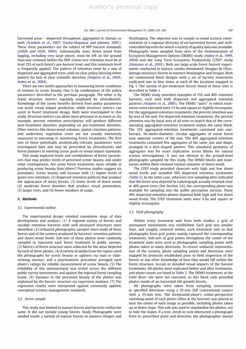
Washington. The objective was to sample in-stand scenery repre-sentative of a regional diversity of un-harvested forests and well-controlled harvests for which a variety of quality data was available.Photographs were sampled from sites of the Demonstration ofEcosystem Management Options (DEMO) study (Aubry et al., 1999,2004) and the Long Term Ecosystem Productivity (LTEP) study(Homann et al., 2001). Both are large-scale forest harvest experi-ments conducted in mature, conifer-dominated, Douglas fir (Pseu-dotsuga menziessi) forests in western Washington and Oregon. Bothare randomized block designs with a set of harvest treatmentsreplicated one to four times at each of the locations mapped inFig. 1. The variety of pre-treatment forests found at these sites isdescribed in Table 1.

The DEMO study provided examples of 15% and 40% retentionharvests, each with both dispersed and aggregated retentionpatterns (Halpern et al., 2005). The DEMO ‘‘units’’ in which treat-ments were executed were 13 ha and square or slightly rectangular.For the aggregated-retention treatments, the percent retention wasby area of the unit. For dispersed retention treatments, the percentretention was by basal area of all trees to match that of the corre-sponding aggregated-retention treatment within the same block.The 15% aggregated-retention treatments contained two one-hectare, 56-meter-diameter, circular aggregates of uncut forestnear opposite corners of the unit. The 40% aggregated-retentiontreatments contained five aggregates of the same size and shape,arranged in a dice-shaped pattern. This unnatural geometry ofaggregates was for exact replication across blocks for naturalscience investigations. It was not obvious in the ground-levelphotographs sampled for this study. The DEMO blocks and treat-ments within them retained various amounts of down wood.

The LTEP study provided clearcuts with high and low downwood levels and included 50% dispersed retention treatments(Table 2). In the latter case, wherever tree sampling plots indicatedthat the forest area depicted in a photograph actually retained closeto 40% green trees (See Section 3.6), the corresponding photo wasavailable for sampling into the public perception surveys. These40% dispersed-retention photos depicted both high and low downwood levels. The LTEP treatment units were 6 ha and square orslightly rectangular.

3.3. Field photography

Within every treatment unit from both studies, a grid ofpermanent monuments was established. Each grid was smallerthan, and roughly centered within, each treatment unit so thatphotographs from grid points mainly captured the correspondingtreatments. Sub-sets of grid points throughout the center of thetreatment units were used as photographic sampling points withphotos taken in many directions. To ensure unbiased representa-tion of the scenery, photo sampling points and directions weremapped by protocols established prior to field inspection of theforests or any other knowledge of how they would fall within theforest structure, terrain or detailed visual impacts of the harvesttreatments. All photos were replicated before and after treatments,and photo counts are listed in Table 2. The DEMO treatments at theLittle River site were not executed, so this block only providedphotos inside of un-harvested old-growth forests.

All photographs were taken from sampling monumentsin specified directions using a 35 mm SLR conventional camerawith a 35 mm lens. The foreground-plane’s center-perspectivevanishing-point of each photo (often at the horizon) was placed asnear the center of each image as possible, including photos takenup or down slope. This rule was used to standardize the photos, notto hide the slopes. If a tree, shrub or rock obstructed a photographfrom its prescribed point and direction, the photographer moved

R.G. Ribe / Journal of Environmental Management 91 (2009) 245–260 247


up to one meter in the shortest possible distance in any directionnecessary to minimize the obstruction to the photograph. Photo-graphs were taken within 3 h of noon, standard time. Pre-treat-ment photos were taken during the same three-month field seasonas corresponding vegetation structure measurements. Post-treat-ment photos were taken within 6 months after treatments werecompleted, and most often within 3 months.

A set pattern of eight grid points was used for photo samplingnear all the edges of every DEMO unit’s central grid of monu-ments. One photo was taken at each point in its own uniquepreset direction toward the middle of the unit. This yielded 48photos of each treatment across the six study blocks. This patternof photos was determined for representative sampling of scenerywithin the 40%, aggregated-retention treatment. This treatmentdetermined the photography protocol because it presented special

problems in representative sampling of its most complex patternof post-harvest scenery. The pattern of photographs was selectedby reference to the pattern of felling relative to the sampling gridfor this 40%, aggregated-retention treatment. The photo pointsand directions captured views inside aggregates, across largerareas of harvested matrix, looking at harvested matrix betweenaggregates, near aggregates with harvested matrix in theforeground, and looking out from just inside aggregates (Tonneset al., 2004). This overall mix of photos sought to capture viewsof harvested matrix and retained aggregates in approximateproportion to that encountered hiking through the wholetreatment.

There were five preset photo sample points within each LTEPtreatment unit. Four photos were taken from each of these in thecardinal compass directions, yielding 20 photos per unit.

Fig. 1. Locations of the ten experimental sites. DEMO study blocks are denoted by circles: CF¼ Capitol Forest, BU¼ Butte, PH¼ Paradise Hills, LW¼ Little White Salmon,WF¼Watson Falls, DP¼Dog Prairie, LR¼ Little River. LTEP study sites are denoted by squares: SP¼ Sappho (2 blocks used), IB¼ Isolation Block (3 blocks), SK¼ Siskiyou (3 blocks).



3.4. Down wood photo sampling

Post-treatment photo samples needed to be sorted by theirdepiction of high versus low down wood within each treatment.Pre-treatment photos were not sorted by down wood level. Sortingwas done by different rules depending on the source study forphotos, as follows.

Down wood volume data were not available for the LTEP units atthe Sappho and Isolation blocks, but the harvests there wereintentionally executed to leave substantially different high versuslow down wood levels as a key part of this study’s protocol. Highdown wood LTEP post-treatment photos were those taken in unitswhere most harvest residue, including tops, limbs, and many logsremained on site, yielding samples of 160 high down photos for bothclearcut and 50% dispersed retention treatments (Table 2). Lowdown wood LTEP photos came from other LTEP units, wherein mostdown wood was substantially removed at harvest, again yieldingsamples of 160 low down wood photos for the same two treatments(Table 2). Among the 50% dispersed-retention photos, 31 high downwood photos and 22 low down wood photos actually depicted 40%retention and became candidates for use in public surveys.

Down wood volume data were available for all DEMO units. Tostandardize the measures of down wood levels between the LTEPand DEMO studies, volume thresholds for sorting DEMO post-treatment photos were calibrated from down wood volume dataavailable for the units at the LTEP Siskiyou blocks. Among photosthat depicted a foreground of 15% dispersed retention, or of har-vested matrix within aggregated-retention treatments, those withmore than 300 m3/ha of down wood were classified as high downwood. For photos depicting 40% dispersed retention harvests, thethreshold was 200 m3/ha because fewer harvested trees producedless down wood even when most such wood was left behind. Forpost-treatment photos depicting foreground un-harvested aggre-gates, the threshold value was 100 m3/ha because little down woodfrom harvesting would find its way inside of these aggregates to beleft there.

Down wood levels in post-treatment DEMO photos were iden-tified by field measurements taken within the area depicted byeach photo, yielding sample-based estimates of the volume ofcoarse wood, course litter, and count of snags leaning more than15� per ha. The course wood (>10 cm diameter) estimates camefrom the 6 m transect shown in the photo and closest to the photo

Table 1Selected features and pre-treatment structural characteristics of forests at the ten study sites.

Source study/Site name

Elevation(m)

Slope(deg)

Stand. age(yr)

Basal area(m2/ha)

Tree density(no./ha)

Quadratic meandiameter (cm)

No. studyreplicate blocks

DEMO studya

Watson falls 945–1310 4–7 110–130 36–52 310–500 39.3 1Little river 1220–1400 14–40 200–520 82–127 255–473 62.6 1Dog Prairie 1460–1710 34–62 165 72–106 258–475 58.1 1Butte 975–1280 40–53 70–80 48–65 759–1781 25.6 1L. white Salmon 825–975 40–66 140–170 61–77 182–335 62.7 1Paradise hills 850–1035 9–33 110–140 59–87 512–1005 36.0 1Capitol forest 210–275 28–52 65 54–73 221–562 48.5 1

LTEP studyb

Sappho 134–147 3–6 52 197–241 778–1864 48.7 2c

Isolation block 482–665 19–48 80–91 53–136 93–962 39.2 3Siskiyou 836–897 12–58 80–106 21–136 280–2700 26.0 3

a Data from trees with a minimum diameter of 5.0 cm.b Data from trees with a minimum diameter of 3.5 cm.c This LTEP site included four replicate blocks but only two were employed in this study due to poor pre-treatment photo quality from the other two.

Table 2Selected visual characteristics of pre-treatment forests, and counts of field photo samples by treatment at the ten study sites.

Source study/site name

Visual penetrationa Ground veg.covera

Amount ofhard woodsa

Number of photos by treatments studiedb

Prtr. 15D 15A 40D 40A CCH CCL 40DH 40DL

DEMO studyc

Watson falls Medium Medium Low 40 8 8 8 8 0 0 0 0Little River High Medium Low Old-growth forests with no treatment (40 photos)Dog Prairie High Low Low 40 8 8 8 8 0 0 0 0Butte Medium Medium Medium 40 8 8 8 8 0 0 0 0L. White Salmon Low Medium High 40 8 8 8 8 0 0 0 0Paradise hills High Low Low 40 8 8 8 8 0 0 0 0Capitol forest Medium High High 40 8 8 8 8 0 0 0 0

LTEP StudySapphod High High Medium 160 0 0 0 0 40 40 40e 40e

Isolation block Low High Medium 240 0 0 0 0 60 60 60e 60e

Siskiyou Low Medium High 240 0 0 0 0 60 60 60e 60e

a Ratings are qualitative and based on inspection of all the photographs taken within each site and serve only to roughly characterize scenic differences.b Abbreviations in list are: Prtr.¼ photos taken prior to forest treatments, 15D¼ 15% dispersed retention, 15A¼ 15% aggregated retention, 40D¼ 40% dispersed retention,

40A¼ 40% aggregated retention, CCH¼ clearcuts with high down wood, CCL¼ clearcuts with low down wood, 40DH¼ 40% dispersed retention with high down wood,40DL¼ 40% dispersed retention with low down wood.

c The DEMO blocks included 75% aggregated-retention treatments not employed in the study here.d The blocks at this site also included treatments with medium down wood levels that were not employed in this study. Half the Sappho treatment units were excluded from

this study due to poor photo quality.e At these sites, only a few photos became candidates for inclusion in the public surveys if they depicted sampling plots where approximately 40% of trees were actually

retained, instead of the 50% overall target retention level over these entire treatment units. These photos augmented the photo sample of the same 40% dispersed retentiontreatments derived from the DEMO blocks.



point. The course litter (5–10 cm diameter) estimates came from six0.2� 0.5 m microplots along the same transect. The leaning snagsestimate came from the 0.08 ha circular plot shown in the photoand closest to the photo point. Leaning, dead trees, not rootedvertical ones, are more likely to adversely affect beauty perceptions(Brush, 1979; Brunson and Shelby, 1992).

3.5. Final photo sampling

A sub-sample was needed from the full set of photos of eachcombination of treatment and down wood level for use in publicsurvey instruments. These sub-samples needed to be small enoughto produce instruments short enough to maximize response ratesand avoid taxing respondents with too many, largely redundantphotographs. The number of sub-sample photos for each treatmenttype needed to reliably represent the scenery found there (Palmerand Hoffman, 2001). A small but reliable sample size was notknown, a priori. Reliability pretests were therefore conducted withsets of 20–40 university students who viewed slides and ratedthem on the same scale as the study’s main surveys. These ratingsessions tested even-numbered sample sizes from four to sixteenphotos, each repeatedly drawn at random from the 48 photos of the40% aggregated-retention treatmentdthe one with the greatestvariety of mixed contrasts between harvested and un-harvestedareas. The variance in average scenic beauty ratings across samplesstabilized at its asymptotically lowest value at twelve or morephotos. The smallest reliable sample size of 12 photos wasemployed to minimize the duration of surveys in order to elicithigher response rates.

Some photos were eliminated from further use. These were offour types: (1) very poor photographic quality; (2) too much plasticflagging in the immediate foreground (used by field researchers);(3) a close-up obstruction (e.g. a tree or shrub) filling more than 25%of the field of view; or (4) taken close to and toward the edge ofa treatment unit (LTEP photos only) so that it mainly depicted thesurrounding forest or a neighboring treatment. This screeningeliminated 9% of DEMO photos and 16% of LTEP photos.

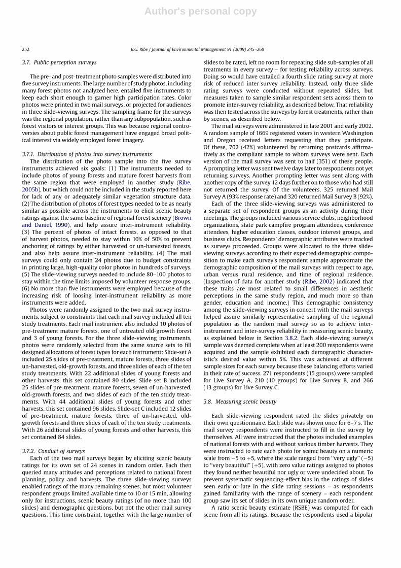
The final sampling of twelve photos for each of the ten studytreatments (n¼ 120) was by random selection. The first sevenphotos selected for each of the ten treatments were joined in thesample by the pre-treatment replicates of the same photos (n¼ 70),so as to sample pre-treatment photos from the same forest typesand sites as the treated photos. To better represent the full range ofpre-treatment forests in the field photo sample, one pre-treatmentphoto was randomly sampled from each of the six DEMO units orLTEP blocks that happened not to be represented by the aboverandom sampling procedure (n¼ 6). This brought the total sampleof un-harvested, mature forest photos to 76. Photos randomlyselected from the old-growth forests at the Little River DEMO site(n¼ 12) joined the sample. This yielded a complete sample of 208photos, as broken down in Table 3. Representative members of thissample are in Fig. 2.

3.6. Measures of stand structure

The main measures of overstory stand structure were basal areaand density of trees and vertical snags per hectare within the forestvisible in each photograph, exclusive of seedlings and shrubs.Density and dbh distributions by species were also analyzed. Thisdata came from pre- and post-treatment vegetation sampling forthe DEMO and LTEP studies, as follows.

The DEMO grid of monuments was placed at 40 m spacing ineach 13 ha treatment unit. Circular 0.04 ha vegetation plots werecentered on a subset of between 32 and 37 of these, depending onthe treatment. The plots were evenly distributed within the

dispersed retention treatments. In the aggregated-retention treat-ments, plots were placed at all grid points inside the aggregates andat an evenly distributed subset of the grid points elsewhere in theharvested matrix areas. Sampling was of all trees greater than 5 cmdbh. Pre-treatment sampling occurred within 4 years prior totreatments and post-treatment sampling occurred in the firstgrowing season after treatment, except at Dog Prairie where hailstripped foliage during the first season.

In the LTEP study, a grid of monuments was placed at 25 mspacing within each 6 ha treatment unit. Five 18� 18 m (.0324 ha)vegetation plots were placed toward the center of each treatmentunit at standardized positions. Sampling was of all trees greaterthan 3.5 cm DBH. Pre-treatment sampling occurred within 3 yearsprior to treatments and post-treatment sampling occurred in thefirst growing season after treatment.

Each study photograph was inspected to estimate the depth ofvisual penetration and identify which vegetation sampling plotswere expected to sample the area visible in the photograph. Thecontent of pre-treatment forest photos was sampled by 1–3 plots.The extent of seen area within post-treatment photos variedgreatly, depending on the level and pattern of green-tree retention,such that 2–8 plots sampled the forests and harvested matrixwithin these photos. One outlier data point, for density at one LTEPSappho photo, was removed using the Dixon–Thompson test(Dixon, 1953) with a 95% confidence interval.

For LTEP photos, tree counts for the smallest 3.5–10 cm dbh classwere adjusted to remove trees between 3.5 and 5 cm to standardizeall photos’ data at the 5 cm dbh threshold employed in the DEMOstudy. This was done by fitting a diameter distribution curve to eachLTEP photo’s data and using the slope of the curve at the smallestdbh range to estimate how many trees were between 3.5 and 5 cmfor subtraction. These corrections were 1–2.5% of total treedensities.

Table 3Key descriptive statistics for mean ratio scenic beauty estimates across the foresttreatments.

Treatment MeanRSBE

Standarddeviation

Standarderror

Numberof scenes

Standarderror asa % of RSBErangeacross allscenesa

Clearcut-lowdown wood

�110.0 20.3 5.8 12 1.9

Clearcut-highdown wood

�109.4 24.6 7.1 12 2.3

15% disp. reten.low dn. wd.

�27.2 38.7 11.2 12 3.6

15% disp. reten.high dn. wd.

�63.7 37.0 10.7 12 3.5

15% agg. reten.low dn. wd.

�31.5 56.2 16.2 12 5.3

15% agg. reten.high dn. wd.

�98.0 40.3 11.6 12 3.8

40% disp. reten.low dn. wd.

74.2 47.4 13.7 12 4.4

40% disp. reten.high dn. wd.

3.5 57.3 16.5 12 5.4

40% agg. reten.low dn. wd.

10.5 95.3 27.5 12 8.9

40% agg. reten.high dn. wd.

�13.1 87.1 25.1 12 8.2

100% reten.mature forest

79.1 33.1 4.3 76 1.4

100% reten.old growth

125.2 32.5 8.4 12 2.7

a The endpoints of the observed range of RSBEs across all study scenes were�157.0 (clearcut with high down wood) and þ176.1 (un-harvested old growth).



Fig. 2. Example public survey photographs of the 12 forest treatments studied.



3.7. Public perception surveys

The pre- and post-treatment photo samples were distributed intofive survey instruments. The large number of study photos, includingmany forest photos not analyzed here, entailed five instruments tokeep each short enough to garner high participation rates. Colorphotos were printed in two mail surveys, or projected for audiencesin three slide-viewing surveys. The sampling frame for the surveyswas the regional population, rather than any subpopulation, such asforest visitors or interest groups. This was because regional contro-versies about public forest management have engaged broad polit-ical interest via widely employed forest imagery.

3.7.1. Distribution of photos into survey instrumentsThe distribution of the photo sample into the five survey

instruments achieved six goals: (1) The instruments needed toinclude photos of young forests and mature forest harvests fromthe same region that were employed in another study (Ribe,2005b), but which could not be included in the study reported herefor lack of any or adequately similar vegetation structure data.(2) The distribution of photos of forest types needed to be as nearlysimilar as possible across the instruments to elicit scenic beautyratings against the same baseline of regional forest scenery (Brownand Daniel, 1990), and help assure inter-instrument reliability.(3) The percent of photos of intact forests, as opposed to thatof harvest photos, needed to stay within 10% of 50% to preventanchoring of ratings by either harvested or un-harvested forests,and also help assure inter-instrument reliability. (4) The mailsurveys could only contain 24 photos due to budget constraintsin printing large, high-quality color photos in hundreds of surveys.(5) The slide-viewing surveys needed to include 80–100 photos tostay within the time limits imposed by volunteer response groups.(6) No more than five instruments were employed because of theincreasing risk of loosing inter-instrument reliability as moreinstruments were added.

Photos were randomly assigned to the two mail survey instru-ments, subject to constraints that each mail survey included all tenstudy treatments. Each mail instrument also included 10 photos ofpre-treatment mature forests, one of untreated old-growth forestand 3 of young forests. For the three slide-viewing instruments,photos were randomly selected from the same source sets to filldesigned allocations of forest types for each instrument: Slide-set Aincluded 25 slides of pre-treatment, mature forests, three slides ofun-harvested, old-growth forests, and three slides of each of the tenstudy treatments. With 22 additional slides of young forests andother harvests, this set contained 80 slides. Slide-set B included25 slides of pre-treatment, mature forests, seven of un-harvested,old-growth forests, and two slides of each of the ten study treat-ments. With 44 additional slides of young forests and otherharvests, this set contained 96 slides. Slide-set C included 12 slidesof pre-treatment, mature forests, three of un-harvested, old-growth forests and three slides of each of the ten study treatments.With 26 additional slides of young forests and other harvests, thisset contained 84 slides.

3.7.2. Conduct of surveysEach of the two mail surveys began by eliciting scenic beauty

ratings for its own set of 24 scenes in random order. Each thenqueried many attitudes and perceptions related to national forestplanning, policy and harvests. The three slide-viewing surveysenabled ratings of the many remaining scenes, but most volunteerrespondent groups limited available time to 10 or 15 min, allowingonly for instructions, scenic beauty ratings (of no more than 100slides) and demographic questions, but not the other mail surveyquestions. This time constraint, together with the large number of

slides to be rated, left no room for repeating slide sub-samples of alltreatments in every survey – for testing reliability across surveys.Doing so would have entailed a fourth slide rating survey at morerisk of reduced inter-survey reliability. Instead, only three sliderating surveys were conducted without repeated slides, butmeasures taken to sample similar respondent sets across them topromote inter-survey reliability, as described below. That reliabilitywas then tested across the surveys by forest treatments, rather thanby scenes, as described below.

The mail surveys were administered in late 2001 and early 2002.A random sample of 1669 registered voters in western Washingtonand Oregon received letters requesting that they participate.Of these, 702 (42%) volunteered by returning postcards affirma-tively as the compliant sample to whom surveys were sent. Eachversion of the mail survey was sent to half (351) of these people.A prompting letter was sent twelve days later to respondents not yetreturning surveys. Another prompting letter was sent along withanother copy of the survey 12 days further on to those who had stillnot returned the survey. Of the volunteers, 325 returned MailSurvey A (93% response rate) and 320 returned Mail Survey B (92%).

Each of the three slide-viewing surveys was administered toa separate set of respondent groups as an activity during theirmeetings. The groups included various service clubs, neighborhoodorganizations, state park campfire program attendees, conferenceattendees, higher education classes, outdoor interest groups, andbusiness clubs. Respondents’ demographic attributes were trackedas surveys proceeded. Groups were allocated to the three slide-viewing surveys according to their expected demographic compo-sition to make each survey’s respondent sample approximate thedemographic composition of the mail surveys with respect to age,urban versus rural residence, and time of regional residence.(Inspection of data for another study (Ribe, 2002) indicated thatthese traits are most related to small differences in aestheticperceptions in the same study region, and much more so thangender, education and income.) This demographic consistencyamong the slide-viewing surveys in concert with the mail surveyshelped assure similarly representative sampling of the regionalpopulation as the random mail survey so as to achieve inter-instrument and inter-survey reliability in measuring scenic beauty,as explained below in Section 3.8.2. Each slide-viewing survey’ssample was deemed complete when at least 200 respondents wereacquired and the sample exhibited each demographic character-istic’s desired value within 5%. This was achieved at differentsample sizes for each survey because these balancing efforts variedin their rate of success. 271 respondents (15 groups) were sampledfor Live Survey A, 210 (10 groups) for Live Survey B, and 266(13 groups) for Live Survey C.

3.8. Measuring scenic beauty

Each slide-viewing respondent rated the slides privately ontheir own questionnaire. Each slide was shown once for 6–7 s. Themail survey respondents were instructed to fill in the survey bythemselves. All were instructed that the photos included examplesof national forests with and without various timber harvests. Theywere instructed to rate each photo for scenic beauty on a numericscale from �5 to þ5, where the scale ranged from ‘‘very ugly’’ (�5)to ‘‘very beautiful’’ (þ5), with zero value ratings assigned to photosthey found neither beautiful nor ugly or were undecided about. Toprevent systematic sequencing-effect bias in the ratings of slidesseen early or late in the slide rating sessions – as respondentsgained familiarity with the range of scenery – each respondentgroup saw its set of slides in its own unique random order.

A ratio scenic beauty estimate (RSBE) was computed for eachscene from all its ratings. Because the respondents used a bipolar



rating scale, the resulting RSBE values took on both positive andnegative values and are scaled to a zero value where the averagerespondent changed from negative (ugly) to positive (beautiful)ratings (Ribe, 1988).

3.8.1. The ratio scenic beauty estimateThe scenic beauty estimation method (SBE, Daniel and Boster,

1976) is established and often used to standardize the dispersion,skewness and central tendency of various respondents’ scenicbeauty ratings to a common, interval scale. It employs a numericresponse scale from 1 to 10 and measures one perceptual construct(scenic beauty) while making no distinction between positiveversus negative scenic beauty. This is problematic in as much as theU.S. Forest Service Scenery Management System (USDA ForestService, 1995) does make this distinction – between levels of beautyand levels of unacceptable modification to scenerydto plan andassess visual impacts. The RSBE is a compromise modification of theSBE that measures a dual construct to serve this need.

The RSBE method standardizes people’s ratings of beauty andugliness onto a common scale. Scenic beauty and ugliness may bethe same cognitive construct that differs only by valence (Torger-son, 1958); or they might be different constructs, each witha cognitively vague zero value. (Indeed, very few respondents inthis study employed the zero rating value on the �5 to þ5 scale.)The RSBE is effectively two SBE scales appended back-to-back, onemeasuring scenic beauty and the other ugliness. The mathematicsof the RSBE is almost identical to the SBE and employs a smallchange to the SBE algorithm (found in Ribe (1988)) that assumesthe distribution of responses across the two scales behave as if onone scale, across a gap at the zero value between very cognitivelysimilar constructs differing by valence. Results from Schroeder(1984) indicate that the scaling and reliability of ratings’ distribu-tions will be very similar on either scale, supporting the likelihoodof a reasonably smooth transition across them. These psychometricuncertainties are offset by the more useful and meaningful valuesthat the RSBE provides for managers.

The zero RSBE value should be understood to apply only withinthe sampling frame of the landscapes investigated because it isuncertain whether it can be compared to such values derivedelsewhere. Consequently, in this study, the RSBE scale, and its zeropoint, is employed only to interpret findings against scenerymanagement standards as applied to the subject region, for whichreliable in-stand forest scene samples were obtained, as describedin Section 3.8.3. This is consistent with scenery managementsystems, which require that visual impacts be judged by referenceonly to the scenic possibilities characteristic of each region.

3.8.2. Reliability across respondent surveysScenic beauty measurement reliability across the five different

survey instruments, particularly between the mail versus slide-viewing surveys, was tested by multiple independent samples chi-square tests. These tests could not employ ratings of the samescenes across the five surveys because surveys did not share scenes.(This was because very many scenes needed to be fit into as fewsurveys as possible to minimize reliability risks and costs associatedwith more surveys, and surveys needed to be short enough tomaximize response rates.) Instead, similar scenes that could beexpected to produce similar RSBEs were employed in the tests.Whenever at least one pre-treatment scene from the same exper-imental block (from the same relatively homogeneous topographyand forest structure) had chanced to be assigned to both mailsurveys and at least two of the slide-viewing surveys, their ratingswere compared, with RSBEs for multiple scenes from the samesurvey averaged. Similarly, whenever at least one scene of the sameclearcut or dispersed retention treatment on mostly level ground

had chanced to be assigned to both mail surveys and at least two ofthe slide-viewing surveys, these were similarly tested for reliabilityacross the surveys. (Photos of these treatments from level sitesacross blocks tended to exhibit the most scenic homogeneity; andphotos of aggregated-retention treatments were too heteroge-neous to expect similar RSBEs across the surveys).

Five forest conditions met these eligibility conditions for chi-squared reliability tests (Table 4). The null hypothesis was that the‘‘true’’ RSBEs for photos of these treatments were nearly the sameacross the surveys, so that no instrument bias could be attributed toany particular survey(s). A moderately stringent critical probabilityvalue of p¼ 0.05 was employed because the somewhat differenttest scenes were not expected to produce identical RSBEs. All fivetests indicated reliable measurement of scenic beauty across theinstruments (Table 4). The signs of the chi-squared test values inTable 4 indicate that slide-viewing surveys produced higher RSBEsin two cases and mail surveys produced higher RSBEs in threecases, discounting the likelihood of a consistent bias, howeversmall, between the two survey modes.

3.8.3. Reliability of scene samplesTable 3 lists the standard error of the mean RSBE of the 12 scenes

representing each forest treatment. These standard errors estimatethe variability expected in mean RSBEs found among other samplesof 12 photos that might be taken from regional examples of eachtreatment. The last column of Table 3 lists these errors asa percentage of the full range of RSBEs observed across all studyscenes. All these values are less than 6% except for the two 40%aggregated-retention treatments, which are less than 9% and forwhich standard errors were minimized as described in Section 3.5.The scene samples are reasonably reliable in representing scenerythat might be produced by the study treatments elsewhere in thestudy region.

3.9. Regression analyses

The regression models reported in Sections 4.2 and 4.3 wereidentified after extensive exploration of variable combinations andmodel specifications to identify the best models for explainingvariance in RSBEs. Models were not estimated using stepwiseprocedures. Only post-hoc stepwise regression was used whenneeded, that forced the final model to be the same as that initiallyestimated without steps. The best models were those that maxi-mized R2; that were most efficient by not including factors who’saddition increased the standard error of estimate; and that onlyincluded factors statistically significant at the 0.10 probability leveland that added at least 0.005 to the R2 (unless such factors hadimportant explicatory value).

4. Analysis and results

4.1. Scope of analysis

This study focused on using attributes of forest structure andtimber harvests to explain scenic beauty inside mature forests ofthe western Pacific Northwest. A repeated-measures study of thescenic effects of the same forest treatments has been publishedelsewhere (Ribe, 2005b) using a larger set of treatments (somewithout forest structure data) and testing treatments’ photosamples representing equal combinations of high and low downwood. A more-robust repeated-measures study could not be con-ducted here because photo samples for each of this study’s foresttreatments included fewer pre-treatment photos (7) than post-treatment photos (12).



4.2. Perceptions of down wood and retention level and pattern afterharvests

Table 3 lists the mean RSBEs for the study treatments. The bestregression model found to explain RSBEs by forest attributesprescribed by New Forestry is in Table 5. That model was estimatedmaking no distinction between mature and old-growth forestsamong 100% retention (no harvest) treatments. All three factorssignificantly explain differences in scenic beauty, and togethersignificantly explain 62% of variance in RSBEs. The standardizedcoefficients indicate that retention level is the strongest predictorof scenic beauty; which is about four times more powerful inexplaining RSBEs than the roughly equal down wood or retentionpattern factors.

The mean RSBEs for the study treatments are graphed in Fig. 3.Their pattern indicates that the RSBEs did discriminate among thetreatments well. This graph exhibits interesting patterns that canbe interpreted to supplement the above interpretation of regres-sion coefficients:

� Down wood level makes no difference in how much ugliness isperceived in clearcuts.

� All four 15% retention treatments are perceived as ugly, butthree of these are seen as significantly less ugly than clearcuts.� The 15% aggregated-retention, high-down-wood treatment is

as ugly as clearcuts.� At 40% retention, only the low-down-wood, dispersed-reten-

tion treatment is seen as decisively beautiful, with about thesame perceived beauty as untreated, mature forests.� The other three 40% retention treatments are perceived to be of

neutral aesthetic value, neither clearly beautiful nor ugly, andnot statistically different from each other.� Down wood level evidently affects aesthetic perceptions more

than retention pattern at the 15% retention level.� Retention pattern is a bit more important than down wood in

affecting RSBEs at the 40% retention level.� The order of perceived beauty of the forest treatments is the

same at both the 15% and 40% retention levels, although thesedifferences are only statistically significant at the extremes, i.e.for the ugliest (aggregated high down wood) 15% retentiontreatment and the most beautiful (dispersed low down wood)40% retention treatment.

Table 4Chi-squared tests of scenic beauty measurement reliability across the five public survey instruments.

Forest treatmentsa Levelclearcuthighdown wood

Level 40% disp.ret. high downwood

Little Riverold-growthforests

Paradise Hillspre-treatmentforests

Sapphopre-treatmentforests

Survey instrument Mean within-instrument RSBE values for the above treatmentsMail survey A �101.5 �43.8 153.5 77.8 75.7Mail survey B �116.1 �27.4 155.3 77.1 82.4Slide-viewing survey 1 �110.0 �35.3 128.0 73.0 60.3Slide-viewing survey 2 �108.4 �47.8 120.7 70.5 59.1Slide-viewing survey 3 �111.1 �33.0 159.2 NAb NAb

Degrees of freedom 4 4 4 3 3Critical Chi-Squared at p¼ .05 �9.49 �9.49 �9.49 �7.81 �7.81Observed Chi-Squared �1.01 �7.28 9.27 0.48 5.75Null hypothesis not rejected,

indicating reliable measurementcYes Yes Yes Yes Yes

a These were the only forest conditions that chanced to be represented in both mail surveys and at least two of the slide-viewing surveys.b Not available because photos of these treatments were not included in slide-viewing survey 3.c The null hypothesis is that the underlying RSBE values are the same for similar photos of the same treatment across the survey instruments. To not reject this hypothesis,

each observed chi-squared value needs to be less than the critical value.

Table 5Regression analysis explaining scenes’ ratio scenic beauty estimates by means ofbasic New Forestry harvest parameters.

Parameter Standardestimate

Standardcoeff.

Error t value Prob.

Intercept �80.33 �80.33 6.16 �13.04 <0.001Retention level 1.74 0.78 0.09 18.64 <0.001Down wood indicatora �21.53 �0.19 4.76 �4.52 <0.001Dispersed retention

indicatorb12.69 0.10 5.46 2.32 0.021

Degrees of freedom R2 Adjusted R2 F-test Prob.

Regression statistics3/204 0.64 0.63 122.20 <0.001

a The down wood indicator variable took on a value of 1.0 for scenes of high-down-wood treatments, -1.0 for scenes of low down wood treatments, and 0 for alluntreated (100% retention) forests with no down wood produced by timberharvesting.

b The dispersed retention indicator variable took on a value of 1.0 for scenes offorest treatments with dispersed patterns of green-tree retention,�1.0 for scenes oftreatments with aggregated green-tree retention, and a value of 0 for clearcuts anduntreated (100% retention) forests. Fig. 3. Mean RSBEs for the forest treatments plotted against retention levels.



� Within either retention level, both low down wood treatmentsare more beautiful than those with high down wood, but thesedifferences are not usually statistically significant.� Within the same down wood level at either retention level, the

dispersed retention pattern is more beautiful than the aggre-gated one, but not usually with statistical significance.� Untreated old-growth forests are perceived as more beautiful

than untreated mature forests.

4.2.1. Reliability of harvest retention patterns in producing scenicbeauty

Some New Forestry treatments may vary in scenic beauty morethan others from one viewpoint to another within a forest, or fromone forest to another. The RSBE standard deviations in Table 3measure the treatments’ reliability of scenic beauty production, andsuggest that aggregated retention and high down wood are asso-ciated with more variation in scenic beauty. Differences were testedin the reliability of scenic beauty production between treatmentsby analyses of variance among these standard deviations (Table 6).Down wood level was never a statistically significant factor in theseANOVAs, indicating more down wood is reliable in reducing scenicbeauty across the treatments. All three effects in this ANOVA arestatistically significant as they explain RSBE standard deviations bythe other two New Forestry parameters. Dispersed retention ismore reliable than aggregated retention in producing expected(average) scenic beauty levels, and this difference is greater at 40%retention than at 15% (Table 6).

4.3. Using forest structure to explain differences in scenic beauty

Percent green-tree retention is only a rough predictor of actualpost-treatment vegetation structure because pre-treatment densi-ties vary considerably, as do decisions about which trees to removein each stand. A number of measures of actual vegetation structurein post- and pre-treatment forests were therefore explored viaregression models to explain variance in forest scenes’ RSBEs.The most singularly efficient were stand density (trees per hectare)and basal area (square meters per hectare) as shown in Tables 7and 8. Quadratic mean diameter (QMD) also proved an effectivemeasure. Density breakdowns by species or by softwood versushardwood trees were unrelated to RSBEs as were counts of leaningsnags. Only the bottom of snags in the foreground of photos werevisible and likely not readily identifiable to respondents as dead treesor ugly. Snags further back in untreated forests and in 40% retentiontreatments often were obscured by live trees. Tree counts in smallerdbh classes were weakly and not significantly related to RSBEs. Thisis likely because there were similarly low counts of small trees inclearcuts, in 15% retention treatments, and in some mature forests;and this study did not include young plantations and young forestswith high densities of small trees. Tree counts in larger dbh classesdid not meet the criteria described in Section 3.9 for inclusion in thebest regression models. QMD proved to be more efficient, significant,

and free of heteroscedasticity errors in modeling the importance oflarger trees in producing scenic beauty.

Basal area proved to be strongly correlated to density (r¼ 0.77)because mature forests with more large trees tend to have more

Table 6Analysis of variance explaining standard deviations of forest treatments’ scenesample RSBEs by means of retention level and pattern, excluding clearcuts and noharvest treatments.a

Source D.f. Mean square F-ratio Prob. Power

Retention level (nominal) 1 1650.25 31.36 0.005 0.98Retention pattern 1 1212.78 23.05 0.009 0.94Ret. pattern X Ret. level 1 404.70 7.69 0.050 0.56

a Data for this analysis are found in Table 3.

Table 7Regression analysis explaining scenes’ ratio scenic beauty estimates by measures offorest structure, here including density, and basic New Forestry harvest parameters.

Parameter Estimate Standardcoeff.

Standarderror

t value Prob.

Intercept �128.35 �128.35 9.57 �13.42 <0.001Density/ha 0.49 1.95 0.07 7.25 <0.001(Density/ha)2 �0.00047 �2.37 0.00012 �3.95 <0.001(Density/ha)3 1.30E-7 0.93 5.26E-8 2.7 0.014Down wood

indicatora�21.37 �0.19 4.94 �4.32 <0.001

Dispersedretentionindicatorb

22.60 0.17 5.72 3.95 <0.001

Quadratic meandiameter

1.34 0.33 0.20 6.76 <0.001



Step Parameter Added R2 Cumulative R2

Stepwise regression explanation of variance in ratio scenic beauty estimates1 Stand density quadratic 0.35 0.352 Quadratic mean diameter 0.21 0.563 Down wood indicator 0.03 0.594 Dispersed retention indicator 0.03 0.62

a The down wood indicator variable took on a value of 1.0 for scenes of high-down-wood treatments,�1.0 for scenes of low down wood treatments, and 0 for alluntreated (100% retention) forests with no down wood produced by timberharvesting.

b The dispersed retention indicator variable took on a value of 1.0 for scenes offorest treatments with dispersed patterns of green-tree retention,�1.0 for scenes oftreatments with aggregated green-tree retention, and 0 for clearcuts and untreated(100% retention) forests.

Table 8Regression analysis explaining scenes’ ratio scenic beauty estimates by measures offorest structure, here including basal area, and New Forestry harvest parameters.

Parameter Estimate Standardcoeff.

Standarderror

t value Prob.

Intercept �108.31 �108.31 8.62 �12.57 <0.001Basal area m2/ha 4.10 2.98 0.36 11.24 <0.001(Basal area m2/ha)2 �0.02 �4.39 0.004 �6.62 <0.001(Basal area m2/ha)3 4.32E-5 1.98 9.77E-6 4.42 <0.001Down wood indicatora �22.70 �0.20 4.54 �5.00 <0.001Dispersed retention

indicatorb24.95 0.19 5.27 4.73 <0.001

Quadratic mean diameter 0.15 0.04 0.20 0.75 0.456



Step Parameter Added R2 Cumulative R2

Stepwise regression explanation of variance in ratio scenic beauty estimates1 Basal area quadratic 0.60 0.602 Down wood indicator 0.04 0.643 Dispersed retention indicator 0.04 0.684 Quadratic mean diameter 0.001 0.68

a The down wood indicator variable took on a value of 1.0 for scenes of high-down-wood treatments,�1.0 for scenes of low down wood treatments, and 0 for alluntreated (100% retention) forests with no down wood produced by timberharvesting.

b The dispersed retention indicator variable took on a value of 1.0 for scenes offorest treatments with dispersed patterns of green-tree retention,�1.0 for scenes oftreatments with aggregated green-tree retention, and 0 for clearcuts and untreated(100% retention) forests.



basal area. Consequently, they could not be included in the samemodel without multicollinearity errors. Each of these factors bestexplained variance in RSBEs via the third-order quadratic specifi-cations illustrated in Figs 4 and 5. Basal area explains substantiallymore variance in RSBEs (R2¼ 0.60 in Table 8) than density(R2¼ 0.35 in Table 7) because it better accounts for the scenic affectof larger trees. This is clear in Fig. 4, where many data points atlower densities occur both well below and above the regressionfunction. Quadratic mean diameter is a needed, significant factoronly in the model employing density (Table 7), where it accountsfor tree sizes. It is not needed in the model employing basal area(Table 8) where basal area adequately accounts for tree size inexplaining scenic beauty. Both these models’ graphs provide esti-mates of optimal vegetation prescriptions for scenic beauty,respectively at about 110–155 m2/ha basal area (Fig. 5) and 700–900 trees/ha (Fig. 4). Figs 4 and 5 show that pronounced increasesin scenic beauty can be expected moving up to these optimalranges, beyond which scenic beauty will likely decline gradually.

The models in Tables 7 and 8 include stepwise regression resultsto aid interpretation of factors’ relative strength, because standard-ized coefficients are difficult to interpret when a factor is expressedvia three quadratic terms. In both models the strongest predictor ofscenic beauty is to approach the optimal basal area or density rangesnoted above. If density is used to model scenic beauty then anotherimportant factor is QMD to account for tree sizes, and this factor canbe omitted from the model using basal area. In both models, reten-tion pattern and down wood levels are useful factors of equal andlesser value in predicting scenic beauty levels.

4.4. Interpolating results across retention levels

It is helpful to estimate expected scenic beauty levels acrossa full range of green-tree retention levels and not just at the fourlevels employed in this study. Fig. 6 shows such interpolations. Thefunctions there were found by two steps: First, a regression modelwas estimated for the three factors employed in the regressionmodels in Tables 7 and 8, using the data points’ observed retentionlevels as the independent variable. All three resulting models were

significant at pf< .001 and all intercepts and coefficients weresignificant at pt< .001. They were: Trees/ha¼ 4.73þ 6.12$Ret. Level(r2¼ 0.41); Basal area m2/ha¼�3.46þ1.14$Ret. Level (r2¼ 0.50);and QMD cm¼ 15.13þ1.44$Ret. Level-0.011$(Ret. Level)2

(R2¼ 0.38). Second, these functions were substituted for the cor-responding factors in the models in Tables 5, 7 and 8, along with therequired combinations of the down wood and retention patternindicator variables. The resulting predicted RSBE functions forretention levels 3–97% are graphed in Fig. 6. (The endpoints ofpossible retention are not plotted because there is no retention inclearcuts and no harvest patterns in 100% retention forests.) Theaverage of the three functions is also plotted at lower right in Fig. 6,as an overall estimate of how retention level relates to scenicbeauty.

5. Discussion

5.1. Summary, research needs and limitations

Forest planners can mitigate public controversies byimproving scenic beauty. They can substantially predict average,relative scenic beauty levels within such forests by readilymeasurable and manageable factors. All the postulates in Section2.2 about how to do so were confirmed, except the last regardingsnags. Increased scenic beauty can be expected, in order ofimportance, with: dispersed rather than aggregated harvestretention patterns, higher harvest retention levels, moderate treedensity, larger trees and less down wood. These factors areconsistent with public preferences for forests with more coher-ently natural scenery (Ode et al., 2009). Dispersed retentionpatterns are more reliable in producing expected aesthetic resultsthan aggregated patterns. More research is needed aboutharvests’ long-term impacts (Shelby et al., 2003) with understoryand tree re-growth, and how aesthetic perceptions relate topeople’s values (Ford et al., 2009).

This study employed a limited sample of forests, focusing onmature forests and harvests of the same. To see how these casesFig. 4. Estimated regression model of RSBEs as a function of stand density.

Fig. 5. Estimated regression model of RSBEs as a function of stand basal area.



compare to young managed forests and old-growth harvests, seeRibe (2005b). Investigation of more levels and combinations ofsilvicultural parameters is needed, particularly to model scenicbeauty inside young forests between 5 and 70 years old. The resultsprovide useful predictions due to the use of reliably measuredforest metrics and scenic beauty, and the extensive sample ofdiverse forests, scenes, and public respondents. The interpretationsin Sections 5.2–5.4 are made from the mean values and theregression functions from this study that offer evidence-basedpredictions of average differences in in-stand scenic beauty. Thesepredictions are subject to the ranges of uncertainty indicated by theerrors graphed in Figs. 3–6.

5.2. Scenic beauty in mature forests

The most efficacious way of achieving scenic beauty in matureforests is by basal area, particularly at lower forest densities. Thecloser forests approach 110–155 m2/ha basal area the more

beautiful they will tend to be. If circumstances entail an emphasison forest density, a useful but less effective strategy is to manageforests toward 700–900 trees/ha and to increase average tree size.These two routine measures of forest structure, alone or together,provide good rules of thumb, while infrequently measured factors,such as vegetative ground cover or vision-blocking shrubs andseedlings, likely also affect forests’ scenic beauty.

5.3. Scenic beauty in timber harvests

The relative importance of factors that explain perceptionsof post-harvest scenic beauty varied among the models in thisstudy, and these are systematically resolved in Section 5.4. But,there is a general consensus across the models shown in Fig. 6.The strongest rule is that the greater the level of post-harvestgreen-tree retention the greater the scenic beauty. Clearcuts areperceived as very ugly irrespective of the level of post-treatmentdown wood (Fig. 3). Dispersed retention patterns are more

Fig. 6. Interpolated plots of the three scenic beauty regression models across harvest retention levels, and a plot of the functional average of these three models.



reliable at producing expected scenic beauty levels than aggre-gated patterns, particularly at higher retention levels, producingfewer ugly ‘‘surprises’’.

At lower levels of green-tree retention, such as 15%, reducingdown wood levels is the most important factor in improving scenicbeauty, but such harvests will still be seen as ugly. Such harvestshave become more common in the U.S. Pacific Northwest, and thismay prove problematic for perceptions of public forests there. Forexample, harvests substantially exhibiting 15% aggregated reten-tion and substantial down wood are not an uncommon NFPprescription and these are seen as not much less ugly than clear-cuts. 15% retention harvests with low down wood and dispersedretention are significantly less ugly than clearcuts, but still ugly.

At higher levels of retention, such as 40%, favoring dispersedinstead of aggregated retention patterns is the most importantfactor in producing scenic beauty. Reduced post-harvest downwood levels are also effective. Dispersed, 40% retention, low-down-wood harvests are seen as beautiful, on average, as the average, un-harvested, mature forest in the region. Other 40% retentionprescriptions are perceived to be scenically neutral, neither beau-tiful nor ugly.

As shown in Fig. 6 across retention levels, dispersed-retention,low-down-wood harvests are estimated to exhibit the highestcomparative scenic beauty, aggregated-retention, high-down-wood harvests tend to have the lowest relative scenic beauty, withother harvests in-between. To further refine scenic beautyproduction, particularly when employing dispersed retentionharvest patterns, silviculturists may aim for the basal area anddensity targets described in Section 4.3, which may often beachievable at 40% retention. If only one of these optimum rangescan be approached, that for basal area is more effective. Retaininglarger trees increases scenic beauty and the basal area target mayoften be achieved at silviculturally desired post-harvest densities.

5.4. Interpretations against conceptual visual impact standards

The findings in Sections 5.2 and 5.3 can be usefully interpretedfor forest planners by an evidence-based, approximate translationto reference VRM standards (USDA Forest Service, 1995; British

Columbia Ministry of Forests, 2001). This entails a rough interpre-tation of numeric RSBE ranges to correspond to VRM standards’conceptual definitions. This is not scientific interpretation buta way to make this study meaningful to planners and impactanalysts who must use VRM methods and need such a translationof the findings. The RSBE ranges corresponding to VRM standardsare explained below by reference to the USDA definitions, are listedin Table 9, and shown in the vertical divisions of Figs. 3–6. In eachcase, the New Forestry parameters studied here are discussed, butmanagers may also seek to target the densities or basal areas inTable 9. The relationship between retention levels and VRM stan-dards is contingent on retention patterns and down wood, asshown in Figs 3 and 6.

5.4.1. High or retention scenic qualityThe reference scenic standard is the ‘‘high’’ scenic integrity level

(USDA) or corresponding ‘‘retention’’ scenic quality class (BCMF).This standard includes forests where ‘‘the valued visual characterappears intact.’’ This is consistent with the range of scenic beautyobserved for mature, un-harvested forests, or the RSBE range of onestandard deviation (33.0) on either side of the mean (79.1) for theuntreated, mature forest scenes in the study (Table 9). Managersseeking to implement this high/retention scenic standard shouldeither extend rotations without harvesting, or employ harvestswith dispersed retention patterns that retain 40% or more treeswith low down wood levels (Fig. 6), closely consistent with findingsin BCMF (1997).

5.4.2. Very high or preservation scenic qualityThe ‘‘very high’’ scenic integrity level (USDA) or corresponding

‘‘preservation’’ scenic quality class (BCMF) is higher than thatabove. It applies to forests where ’valued scenic character and senseof place is intact and is expressed to the highest possible level.’ Thisis consistent with all RSBE values above the high/retention levelsdiscussed above (Table 9), to include most of this study’s old-growth forest scenes as well as a few mature forest scenes withvery high RSBEs. Such scenery is highly valued as iconic of regionalsense of place (Dietrich, 1992; Durbin, 1996) and for conservation(Ribe and Matteson, 2002). Managers seeking this very-high/

Table 9Rules of thumb identifying the highest scenery management standard for which forest treatments and conditions will typically be acceptable for short-term, in-stand scenicimpacts.

USDA BCMF scenicstandard

ApproxRSBE range

Densityrange trees/haa

B. A. rangem2/hab

Forest treatments from this study that haveacceptable visual impactsc,d

Very high Preservation >112 700–900 with disp.retention & high QMD

110–155 Many old-growth forests, Some mature forests

High Retention 46–112 700 to 900 withdisp. retention

50–110 and >155 Most mature forests, 40% disp.ret.- low dn wd harvests

Moderate Partial retention 0–46 400–1500 30–50 40% disp. ret.- high dn wd harvests40% agg. ret.- low dn wd harvests

Low Modification �90–0 100–400 and >1500 10–30 40% agg. ret.- high dn wd harvests15% disp. ret.- low dn wd harvests15% agg. ret.- low dn wd harvests15% disp. ret.- high dn wd harvests15% agg. ret.- high dn wd harvests

Very low Maximum modification <�90e 0–100e 0–10e Clearcut-low-down-wood harvestse

Clearcut-high-down-wood harvestse

Unacceptably low Unaccept. modific. <�90e 0–100e 0–10e Clearcut-low down wood harvestse

Clearcut-high-down-wood harvestse

a Ranges are estimated from the fitted curve in Fig. 4 and are subject to the errors shown there.b Ranges are estimated from the fitted curve in Fig. 5 and are subject to the errors shown there.c Threshold values for high down wood were 300 m3/ha for clearcuts, all 15% retention harvests, and 40% aggregated-retention harvests (within the harvested matrix area);

and 200 m3/ha for 40% dispersed retention harvests.d Interpretations in this column are made by reference to the lower-right graph in Fig. 6, with cross-reference to Figs. 3–5, and are subject to the errors shown in all three of

these figures.e The application of the very low versus unacceptably low scenic impact standard to forests in this RSBE range is a matter of policy choice that can not be interpreted from

the results of this study.



preservation scenic standard should retain old-growth forests andretain or treat mature and old forests to approach the density andbasal area ranges indicated in Table 9.

5.4.3. Moderate or partial retention scenic qualityThe ‘‘moderate’’ scenic integrity level (USDA) or corresponding

‘‘partial retention’’ scenic quality class (BCMF) is just below thehigh/retention standard discussed in Section 5.4.1. It applies toforests where valued scenic character ‘‘appears slightly altered’’ andwhere ‘‘noticeable deviations must remain visually subordinate’’ tothe valued forest character. This is consistent with forest scenerythat is aesthetically impacted by disturbances but remains ofpositive perceived scenic beauty, corresponding to the range ofRSBEs below that for high/retention but above the zero RSBE value(Table 9). Managers seeking to just meet this moderate/partial-retention scenic standard should employ harvests of 20–40%retention (Fig. 6), either in a dispersed pattern with high downwood, or an aggregated pattern with low down wood. BritishColumbia Ministry of Forests (1997) found that 20% is the minimumgreen-tree retention level needed to potentially meet thismoderate/partial-retention standard in the dispersed-retention,low-down-wood forests they studied, and this is closely corrobo-rated by the 17% retention level indicated for this transition point insuch forests in the lower-right graph of Fig. 6.

5.4.4. Low or modification scenic qualityThe ‘‘low’’ scenic integrity level (USDA) or corresponding

‘‘modification’’ scenic quality class (BCMF) is just below themoderate/partial-retention standard discussed above. It applies toforests where valued scenic character ‘‘appears moderately altered’’and ‘‘deviations begin to dominate’’ the scenery. Such deviationsfrom valued forest scenery should nevertheless be ‘‘compatible orcomplimentary’’ to such scenery. This can be interpreted asconsistent with negative RSBEs but only for scenes that retainvisually clear forest attributes, i.e. those derived from at least somesignificant green-tree retention. The lower limit of this moderate/partial-retention RSBE range can reasonably be set at an RSBE valueof �90 (Table 9), just above which almost all scenes were awardedwith ratings of �2 or higher by at least a majority of studyrespondents. Managers seeking to just meet this low/modificationscenic standard may employ 40% aggregated-retention harvestswith high down wood, or any of the 15% retention harvests studiedhere (Table 9), similar to BCMF’s (1997) less than 20% retentionfinding.

5.4.5. Very low or maximum-modification scenic qualityThe ‘‘very low’’ scenic integrity level (USDA) or ‘‘maximum

modification’’ scenic quality class (BCMF) is below the low/modi-fication standard above. It applies to forests where valued sceniccharacter ‘‘appears heavily altered’’ and where ‘‘deviations stronglydominate.’’ This can be interpreted as consistent with RSBEs below�90 (Table 9), below which a majority of respondents almostalways awarded scenes with ratings of �3 to �5. Managerspermitted to meet this very-low/maximum-modification scenicstandard may employ clearcuts with any level of down wood. Thisvery low perceived scenic beauty might instead be interpreted asconsistent with the lowest possible ‘‘unacceptably low’’ (USDA) or‘‘unacceptable modification’’ (BCMF) standard, which would renderclearcuts impermissible anywhere subject to scenic standards.

Acknowledgments

This study was mainly supported by the Demonstration ofEcosystem Management Options (DEMO) project, a joint effort of

the USDA Forest Service Region 6 and Pacific Northwest ResearchStation. Research partners include the University of Washington,Oregon State University, University of Oregon, Gifford Pinchot andUmpqua National Forests, and the Washington State Department ofNatural Resources. Valuable assistance was provided by TerryDaniel, John Nakae, Rick Abbott, Robyn Darbyshire, Charlie Halpern,Bernard Bormann, Tony Silvaggio, Keith Aubry, George Stankey,Bruce Shindler, Tim Max, Kath Williams, Jim Overton, WayneKleckner, Mike Amaranthus, Jim Boyle, Rebecca Ford, BrendaWoodard, Richard Bigley, Dan Terrel, Brian York, Will Kaye, DavidElkin, Richard Campbell-Mayer, Charles Peterson, Cindy Lagouda-kis, Patty Gwartney, Al Horton, Debbie Couche, Gabe Tucker, GodySpycher, Rick Chenoweth, and the staff of the Oregon SurveyResearch Laboratory.

References

Alho, J.M., Kangas, J., 1997. Analyzing uncertainties in experts’ opinions of forestplan performance. For. Sci. 43, 521–528.

Arthur, L.M., 1977. Predicting scenic beauty of forest environments: some empiricaltests. For. Sci. 23, 151–159.

Aubry, K.B., Amaranthus, M.P., Halpern, C.B., White, J.D., Woodard, B.L.,Peterson, C.E., Lagoudakis, C.A., Horton, A.J., 1999. Evaluating the effects ofvarying levels and patterns of green-tree retention: experimental design of theDEMO study. Northwest Sci. 73 (Special issue), 12–26.

Aubry, K.B., Halpern, C.B., Maguire, D.A., 2004. Ecological effects of variable reten-tion harvests in the northwestern United States: the DEMO study. Forest SnowLandsc. Res. 78, 119–137.

Benson, R.E., Ullrich, J.R., 1981. Visual Impacts of Forest Management Activities:Findings on Public Preferences. Research Paper INT-262. USDA Forest Service,Logan, UT.

Bliss, J.C., 2000. Public perceptions of clearcutting. J. Forest. 98 (12), 4–9.Bormann, B.T., Cunningham, P.G., Brookes, M.H., Manning, V.W., Collopy, M.W.,

1994. Adaptive Ecosystem Management in the Pacific Northwest. GeneralTechnical Report PNW-341. USDA Forest Service, Portland, OR.

Bradley, G.A., Kearney, A.R., Wager, J.A., 2004. Public reactions research. In:Curtis, R.O., Marshall, D.D., DeBell, D.S. (Eds.), Silvicultural Options for YoungGrowth Douglas-fir Forests: The Capitol Forest Studyd Establishment and FirstResults. General Technical Report PNW-598. USDA Forest Service, Portland, OR,pp. 63–73.

British Columbia Ministry of Forests, 1997. Visual Impacts of Partial Cutting:Summary Report: A Technical Analysis and Public Perception Study. ForestPractices Branch, Victoria, BC.

British Columbia Ministry of Forests, 2001. Forest Practices Code of BritishColumbia: Visual Impact Assessment Guidebook, second ed. Forest PracticesBranch, Victoria, BC.

British Columbia Ministry of Forests and Range, 2006. The Public Response toHarvest Practices in British Columbia at the Landscape and Stand Level. ForestPractices Branch, Victoria, BC.

Brown, T.C., Daniel, T.C., 1986. Predicting scenic beauty of timber stands. For. Sci. 32,471–487.

Brown, T.C., Daniel, T.C., 1990. Scaling of Ratings: Concepts and Methods. ResearchPaper RM-293. USDA Forest Service, Fort Collins, CO.

Brunson, M.W., Shelby, B., 1992. Assessing recreational and scenic quality: how does’New Forestry’ rate? J. Forest. 90 (7), 37–41.

Brush, R.O., 1976. Spaces within the woods: managing forests for visual enjoyment.J. Forest. 74 (11), 744–747.

Brush, R.O., 1979. The attractiveness of woodlands: perceptions of forest land-owners in Massachusetts. For. Sci. 25, 495–506.

Buhyoff, G.J., Hull IV, R.B., Lien, J.N., Cordell, H.K., 1986. Prediction of scenic qualityfor southern pine stands. For. Sci. 32, 769–778.

Carroll, M., 1995. Community and the Northwestern Logger: Communities andChanges in the Era of the Spotted Owl. Westview Press, Boulder, CO.

Cashore, B., Hoberg, G., Howlett, M., Rayner, J., Wilson, J., 2000. In Search ofSustainability. University of British Columbia Press, Vancouver, BC.

Chokor, B.A., Mene, S.A., 1992. An assessment of preference for landscapes in thedeveloping world: case study of Warri, Nigeria, and environs. J. Environ.Manage. 34, 237–256.

Daniel, T.C., Boster, R.S., 1976. Measuring Landscape Esthetics: The Scenic BeautyEstimation Method. Research Paper RM-167. USDA Forest Service, Fort Collins, CO.

Debell, D.S., Curtis, R.O., 1993. Silviculture and new forestry in the Pacific North-west. J. Forest. 91 (12), 26–30.

DeVall, B. (Ed.), 1994. Clearcut: The Tragedy of Industrial Forestry. Sierra Club Books,San Francisco.

Dietrich, W., 1992. The Final Forest: The Battle for the Last Great Trees of the PacificNorthwest. Simon and Schuster, New York.

Dixon, W.J., 1953. Processing data for outliers. Biometrics 9, 74–89.Durbin, K., 1996. Tree Huggers: Victory, Defeat, and Renewal in the Northwest

Ancient Forest Campaign. The Mountaineers, Seattle.



Durning, A.T., 1999. Green Collar Jobs: Working in the New Northwest. NorthwestEnvironment Watch, Portland, OR.

Echelberger, H.E., 1979. The semantic differential in landscape research. In:Elsner, G.H., Smardon, R.C. (Eds.), Our National Landscape: Proceedings ofa Conference on Applied Techniques for Analysis and Management of the VisualResource. General Technical Report PSW-35. USDA Forest Service, Berkeley, CA,pp. 524–531.

Ford, R.M., Williams, K.J.H., Bishop, I.D., Webb, T., 2009. A value basis for the socialacceptability of clearfelling inTasmania, Australia. Landsc. Urb. Plann. 90,196–206.

Franklin, J.F., Perry, D.A., Schowalter, T.D., Harmon, M.E., Mckee, A., Spies, T.A., 1989.Importance of ecological diversity in maintaining long-term site productivity.In: Perry, D.A., Meurisse, R., Thomas, B., Miller, R., Boyle, J., Means, J., Perry, C.R.,Power, R.F. (Eds.), Maintaining the Long-term Productivity of Pacific NorthwestForest Ecosystems. Timber Press, Portland, OR, pp. 82–97.

Franklin, J.F., Berg, D.R., Thornburgh, D.A., Tappeiner, J.C., 1997. Alternative silvi-cultural approaches to timber harvesting: variable retention harvest systems.In: Kohm, K.A., Franklin, J.F. (Eds.), Creating a Forestry for the 21st Century: TheScience of Ecosystem Management. Island Press, Washington, DC, pp. 111–139.

Gobster, P.H., 1996. Forest aesthetics, biodiversity, and the perceived appropriate-ness of ecosystem management practices. In: Brunson, M.W., Kruger, L.E.,Tyler, C.B., Schroeder, S.A. (Eds.), Defining Social Acceptability in EcosystemManagement: A Workshop Proceedings, General Technical Rep. PNW-669.USDA For. Serv., Portland, OR, pp. 77–97.

Gobster, P.H., 1999. An ecological aesthetic for forest landscape management.Landsc. J. 18, 54–64.

Halpern, C.B., Mckenzie, D., Evans, S.A., Maguire, D.A., 2005. Initial responses offorest understories to varying levels and patterns of green-tree retention. Ecol.Appl. 15, 175–195.

Harmon, M.E., Franklin, J.F., Swanson, F.J., Sollims, P., Gregory, S.V., Lattin, J.D.,Anderson, N.H., Cline, S.P., Aumen, N.G., Sedell, J.R., Lienkaemper, G.W.,Cromack Jr., K., Cummins, K.W., 1986. Ecology of course woody debris intemperate ecosystems. Adv. Ecol. Res. 15, 133–302.

Homann, P.S., Bormann, B.T., Boyle, J.R., 2001. Detecting treatment differences in soilcarbon and nitrogen resulting from forest manipulations. Soil Sci. Soc. Am. J. 65,463–469.

Hull, R.B., Buhyoff, G.J., 1986. The scenic beauty temporal distribution method: anattempt to make scenic beauty assessments compatible with forest planningefforts. For. Sci. 32, 271–286.

Hull, R.B., Buhyoff, G.J., Cordell, H.K., 1987. Psychophysical models: an example withscenic beauty perceptions of roadside pine forests. Landsc. J. 6, 113–122.

Kaplan, R., Kaplan, S., 1989. The Experience of Nature. Cambridge Univ. Press,Cambridge.

Karjalainen, E., 1996. Scenic preferences concerning clear-fell areas in Finland.Landsc. Res. 21, 159–173.

Karjalainen, E., Komulainen, M.,1999. The visual effect of fellingon small- and medium-scale landscapes in north-eastern Finland. J. Environ. Manage. 55, 167–181.

Kim, Y.-S., Wells, A., 2005. The impact of forest density on property values. J. Forest.103 (3), 146–151.

Leskinen, P., Vitanen, J., Kangas, A., Kangas, J., 2006. Alternatives to incorporateuncertainty and risk attitude in multicriteria evaluation of forest plans. For. Sci.52, 304–312.

Liao, W., Nogami, K., 1999. Prediction of near-view scenic beauty in artificial standsof Hinoki. J. Forest. Res. 4, 93–98.

Lindhagen, A., 1996. An approach to clarifying public preferences about silviculturalsystems: a case study concerning group selection and clear-cutting. Scand.J. For. Res. 11, 375–387.

McCool, S.F., Benson, R.E., 1988. Timber harvesting and visual resources: main-taining quality. In: Schmidt, W.C. (Ed.), Proceedings- Future Forests of theMountain West: A Stand Culture Symposium. General Technical Report INT-243. USDA For. Serv., Logan, UT, pp. 117–122.

McDonald, P.M., Litton Jr., R.B., 1998. Combining Silviculture and Landscape Archi-tecture to Enhance the Roadside View. Research Paper PSW-235. USDA For.Service, Berkeley, CA.

McQuillan, A.G., 1993. Cabbages and kings: the ethics and aesthetics of newforestry. Environ. Values 2, 191–221.

Nassauer, J.I., 1995. Messy ecosystems: orderly frames. Landsc. J. 14, 161–171.Niemi, E., Whitelaw, E., 1999. Assessing Economic Tradeoffs in Forest Management.

General Technical Report PNW-403. USDA Forest Service, Portland, OR.Ode, A., Fry, G., Tveit, M.S., Messager, P., Miller, D., 2009. Indicators of perceived natu-

ralness as drivers of landscape preference. J. Environ. Manage. 90 (1), 375–383.Palmer, J.F., Hoffman, R.E., 2001. Rating reliability and representation validity in

scenic landscape assessments. Landsc. Urban Plan. 54, 149–161.Palmer, J.F., 2008. The perceived scenic effects of clearcutting in the White Moun-

tains of New Hampshire, USA. J. Environ. Manage. 89, 167–183.Pukkala, T., Kellomaki, S., Mustonen, E., 1988. Prediction of the amenity of a tree

stand. Scand. J. For. Res. 3, 533–544.Ribe, R.G., 1988. Getting the scenic beauty estimation method to a ratio scale:

a simple revision to assess positive and negative landscapes. In: Lawrence, D.,Habe, R., Hacker, A., Sherrod, D. (Eds.), EDRA 19/1988 People’s Needs/PlanetManagement: Paths to Coexistence. Environmental Design Research Associa-tion, Oklahoma City, OK, pp. 41–47.

Ribe, R.G., 1989. The aesthetics of forestry: what has empirical preference researchtaught us. Environ. Manage. 13, 55–74.

Ribe, R.G., 1990. Understanding the aesthetic perception of northern hardwoodforests: toward a general model of scenic beauty in deciduous forests. Landsc. J.9, 86–101.

Ribe, R.G., 2002. Is scenic beauty a proxy for acceptable management? The influence ofenvironmental attitudes on landscape perceptions. Environ. Behav. 34, 757–780.

Ribe, R.G., Matteson, M.Y., 2002. Views of old forestry and new among referencegroups in the Pacific Northwest. West. J. Appl. Forest. 17, 173–182.

Ribe, R.G., 2005a. Aesthetic perceptions of green-tree retention harvests in vistaviews. The interaction of cut level, retention pattern and harvest shape. Landsc.Urban Plan. 73, 277–293.

Ribe, R., 2005b. Comparing changes in scenic beauty produced by green-treeretention harvests, thinnings and clearcuts: evidence from three PacificNorthwest experiments. In: Peterson, C.E., Maguire, D. (Eds.), BalancingEcosystem Values: Innovative Experiments for Sustainable Forestry. GeneralTechnical Report PNW-635. USDA Forest Service, Portland, OR, pp. 137–146.

Ribe, R.G., 2006. Perceptions of forestry alternatives in the U.S. Pacific Northwest:information effects and acceptability distribution analysis. J. Environ. Psychol.26, 100–115.

Rosenberger, R.S., Smith, E.L., 1998. Assessing Forest Scenic Beauty Impacts ofInsects and Management. Forest Health and Technology Enterprise TeamReport 98-08. USDA Forest Service, Fort Collins, CO.

Rudis, V.A., Gramann, J.H., Westphal, J.M., 1988. Forest inventory and management-based visual preference models of southern pine stands. For. Sci. 34, 846–863.

Rutherford Jr., W., Shafer, E.L., 1969. Selection cuts increased natural beauty in twoAdirondack forest stands. J. Forest. 67 (6), 415–419.

Ryan, R.L., 2005. Social Science to Improve Fuels Management: a Synthesis ofResearch on Aesthetics and Fuels Management. General Technical Report NC-261. USDA Forest Service, Saint Paul, MN.

Schroeder, H.W., Daniel, T.C., 1981. Progress in predicting the perceived scenicbeauty of forest landscapes. For. Sci. 27, 71–80.

Schroeder, H.W., 1984. Environmental perception rating scales: a case for simplemethods of analysis. Environ. Behav. 16, 573–598.

Schweitzer, D.L., Ullrich, J.R., Benson, R.E., 1976. Esthetic Evaluation of TimberHarvesting in the Northern Rockies: A Progress Report. Research Note INT-203.USDA Forest Service, Logan, UT.

Shelby, B., Thompson, J.M., Brunson, M., Johnson, R., 2003. Changes in scenic qualityafter harvest: a decade of ratings for six silviculture treatments. J. Forest. 101(2), 30–35.

Sheppard, S.R.J., 2001. Beyond visual resource management: emerging theories ofan ecological aesthetic and visible stewardship. In: Sheppard, S.R.J.,Harshaw, H.W., McBride, J.R. (Eds.), Forests and Landscapes: Linking Ecology,Sustainability and Aesthetics. CABI Publishing, New York, pp. 149–172.

Sheppard, S.R.J., 2003. Knowing a socially sustainable forest when you see one:implications for results-based forestry. Forest. Chron. 79, 865–875.

Sheppard, S.R.J., Harshaw, H.W., McBride, J.R., 2001. Priorities for reconcilingsustainability and aesthetics in forest landscape management. In: Sheppard, S.R.J.,Harshaw, H.W., McBride, J.R. (Eds.), Forests and Landscapes: Linking Ecology,Sustainability and Aesthetics. CABI Publishing, New York, pp. 263–288.

Shindler, B.A., Brunson, M., Stankey, G.H., 2002. Social Acceptability of ForestConditions and Management Practices: A Problem Analysis. General TechnicalReport PNW-537. USDA Forest Service, Portland, OR.

Silvennoinen, H., Alho, J., Kolehmainen, O., Pukkala, T., 2001. Prediction models oflandscape preferences at the forest stand level. Landsc. Urban Plan. 56, 11–20.

Silvennoinen, H., Pukkala, T., Tahvanainen, L., 2002. Effect of cuttings on the scenicbeauty of a tree stand. Scand. J. For. Res. 17, 263–273.

Stark, N.M., 1988. Nutrient cycling concepts as related to stand culture. In:Schmidt, W.C. (Ed.), Proceedings – Future Forests of the Mountain West: AStand Culture Symposium. General Technical Report INT-243. USDA ForestService, Logan, UT, pp. 210–218.

Swanson, F.J., Franklin, J.F., 1992. New forestry principles from ecosystem analysis ofPacific Northwest forests. Ecol. Appl. 2, 262–274.

Tonnes, S., Karjalainen, E., Neuvonen, M., 2004. Scenic impacts of retention trees inclear-cutting areas. Scand. J. For. Res. 19, 348–357.

Torgerson, W.S., 1958. Theory and Methods of Scaling. Wiley, New York, pp. 194–201.Tveit, M.S., 2009. Indicators of visual scale as predictors of landscape preference;

a comparison between groups. J. Environ. Manage. 90, 2882–2888.USDA, USDI, 1994. Record of Decision for Amendments to Forest Service and Bureau

of Land Management Planning Documents Within the Range of the NorthernSpotted Owl: Standards and Guidelines for Management of Habitat for Late-successional and Old-growth Forest Related Species Within the Range of theNorthern Spotted Owl. Interagency SEIS Team, Portland, OR.

USDA Forest Service, 1995. Landscape Aesthetics: A Handbook for SceneryManagement. USDA Handbook 701, Washington, DC.

Vanha-Majamaa, I., Jalonen, J., 2001. Green tree retention in Fennoscandian forestry.Scand. J. For. Res. (Suppl. 3), 79–90.

Vodak, M.C., Roberts, P.L., Wellman, J.D., Buhyoff, G.J., 1985. Scenic impacts ofeastern hardwood management. For. Sci. 31, 289–302.

Yaffee, S.L., 1994. The Wisdom of the Spotted Owl: Policy Lessons for a New Century.Island Press, Washington, DC.
