author's personal copy · the transims population synthesizer uses ipf for the generation of...

This article appeared in a journal published by Elsevier. The attachedcopy is furnished to the author for internal non-commercial researchand education use, including for instruction at the authors institution

and sharing with colleagues.

Other uses, including reproduction and distribution, or selling orlicensing copies, or posting to personal, institutional or third party

websites are prohibited.

In most cases authors are permitted to post their version of thearticle (e.g. in Word or Tex form) to their personal website orinstitutional repository. Authors requiring further information

regarding Elsevier’s archiving and manuscript policies areencouraged to visit:

http://www.elsevier.com/authorsrights

http://www.elsevier.com/authorsrights

Author's personal copy

Disaggregating heterogeneous agent attributes and location

Ying Long a,⇑, Zhenjiang Shen b

a Beijing Institute of City Planning, Beijing 100045, Chinab School of Environment Design, Kanazawa University, Kanazawa 920-1192, Japan

a r t i c l e i n f o

Article history:Received 12 May 2011Received in revised form 27 August 2013Accepted 9 September 2013Available online 8 October 2013

Keywords:Agent-based models (ABMs)DisaggregationPopulation synthesisAggregate dataAgenter

a b s t r a c t

The use of micro-models as supplements for macro-models has become an accepted approach into theinvestigation of urban dynamics. However, the widespread application of micro-models has been hin-dered by a dearth of individual data, due to privacy and cost constraints. A number of studies have beenconducted to generate synthetic individual data by reweighting large-scale surveys. The present studyfocused on individual disaggregation without micro-data from any large-scale surveys. Specifically, a ser-ies of steps termed Agenter (a portmanteau of ‘‘agent producer’’) is proposed to disaggregate heteroge-neous agent attributes and locations from aggregate data, small-scale surveys, and empirical studies.The distribution of and relationships among attributes can be inferred from three types of existing mate-rials to disaggregate agent attributes. Two approaches to determining agent locations are proposed hereto meet various data availability conditions. Agenter was initially tested in a synthetic space, then verifiedusing the acquired individual data, which were compared to results generated using a null model. Agen-ter generated significantly better disaggregation results than the null model, as indicated by the proposedsimilarity index (SI). Agenter was then used in the Beijing Metropolitan Area to infer the attributes andlocation of over 10 million residential agents using a census report, a household travel survey, an empir-ical study, and an urban GIS database. Agenter was validated using micro-samples from the survey, withan average SI of 72.6%. These findings indicate the developed model may be suitable for using in thereproduction of individual data for feeding micro-models.

� 2013 Elsevier Ltd. All rights reserved.

1. Introduction

Micro-models using individual-level data, such as agent-basedmodels (ABMs) and microsimulation models, have been discussedincreasingly in the context of regional, urban, and population stud-ies as supplements to traditional macro-models (Wu, Birkin, &Rees, 2008). However, the use of micro-models has been hinderedby the poor availability of individual data due to privacy and costconstraints. To rectify this hindrance, a number of studies havebeen conducted to generate synthetic individual data by reweigh-ting large-scale surveys. This study focused on individual disaggre-gation without micro-data from large-scale surveys. This situationis common in developing countries like China, Southeast Asiancountries, South American countries, and African countries. Specif-ically, a series of steps were proposed to disaggregate heteroge-neous agent attributes and locations from aggregate data, small-scale surveys,1 and empirical studies. These disaggregated resultscould be used as input for ABMs and microsimulation models. Micro-simulation models tend to pay attention to micro-data based on

policy evaluation (such as taxes, insurance, and health). ABMs focusmore on exploring emerging phenomena at the macro-level, usinginteractions among agents, simple behavior rules, and interactionsbetween agents and their environment. In this paper, the term ABMsis used, but the present approach also applies to microsimulationmodels.

Conditions of micro-data availability can be divided into threelevels. The first level involves sufficient micro-data for ABMs.Such conditions occur in areas like Sweden, where original sur-veyed micro-data can be freely accessed (Holm, Lindgren, Makila,& Malmberg, 1996). The study conducted by Benenson et al. in Is-rael also fit the criteria for the first level (2002). Householderagents were conducted using the 1995 Population Census of Is-rael. The second level includes surveyed samples, such as theUK. Sample of Anonymised Records (SARs) and the U.S. Censusof 2000. These samples can be used to feed agents in ABMs di-rectly or after necessary reweighting (synthetic creation), as instudies conducted by Birkin, Turner, and Wu (2006) and Smith,Clarke, and Harland (2009). The third level is the absence oflarge-scale micro-data for initializing ABMs. Such conditions existin regions in which only statistical yearbooks or census reportswith aggregate information of surveys are published, such as inChina and other developing countries. The ABM constructed byLi and Liu was constructed at this level (2008).

0198-9715/$ - see front matter � 2013 Elsevier Ltd. All rights reserved.http://dx.doi.org/10.1016/j.compenvurbsys.2013.09.002

⇑ Corresponding author. Tel.: +86 10 8807 3660.E-mail address: [email protected] (Y. Long).

1 In this paper, surveys with a sampling ratio of less than 2% and incompleteattributes are defined as small-scale surveys.

Computers, Environment and Urban Systems 42 (2013) 14–25

Contents lists available at ScienceDirect

Computers, Environment and Urban Systems

journal homepage: www.elsevier .com/locate /compenvurbsys


Individual disaggregation has been discussed in the field of pop-ulation studies, especially population synthesis, which is used togenerate synthetic individual data for microsimulation modelsusing aggregate data. Synthetic construction and reweighting aretwo dominant approaches to individual disaggregation, as demon-strated by Hermes and Poulsen reviewed current methods forreweighting (2012). Müller and Axhausen reviewed a list of popu-lation synthesizers, including PopSynWin, ILUTE, FSUMTS, CEM-DAP, ALBATROSS, and PopGen (2010). The iterative proportionalfitting (IPF) techniques2 adopted by PopGen, were first proposedby Deming and Stephan (1940), and comprise one of the most widelyused methods for population synthesis. IPF, which involves reweigh-ting, can adjust tables of data cells so they add up to selected totalsfor both the columns and rows (in two-dimensional cases). Theunadjusted data cells are referred to as seed cells, and the selectedtotals are referred to as marginal totals. Fienberg used IPF to com-bine multiple censuses into a single table (1977).

IPF is a mathematical procedure originally developed to com-bine information from two or more datasets. It can be used whenthe values in a table of data are inconsistent, or when row andcolumn totals have been obtained from different sources(Norman, 1999). Birkin et al. developed the Population Recon-struction Model to recreate 60 million individuals reweightedfrom the U.K. Sample of Anonymised Records (SARs) (2006). Itprovides 1% micro-data describing U.K. households. Wu et al. sim-ulated student dynamics in Leeds, United Kingdom, based on thesynthetic population using the Population Reconstruction Modeland an integrated approach of microsimulation and ABM (2008).Smith et al. (2009) proposed a method for improving the processof synthetic sample generation for microsimulation models(2009). The TRANSIMS population synthesizer uses IPF for thegeneration of synthetic households with demographic character-istics in addition to the placement of each synthetic householdon a link in a transportation network and assigning vehicles toeach household (Eubank et al., 2004). However, these previousstudies were primarily conducted to generate individuals basedon existing large scale micro-samples, namely through reweigh-ting, with the exception of Barthelemy and Toint, whose workwas used to produce a synthetic population for Belgium at themunicipality level without a sample (2013). In the present study,generating agents were investigated on a fine scale without anylarge-scale individual samples.

The present work focused on disaggregating agents with heter-ogeneous attributes and locations based on both attribute informa-tion and spatial location information stored in existing datasources. With respect to agent location, studies regarding the map-ping of population distribution were considered useful (Langford &Unwin, 1994; Liao, Wang, Meng, & Li, 2010; Mennis, 2003). In thesestudies, population density can be interpolated using spatial fac-tors and population census data. However, these studies did notconsider the disaggregation of population attributes. Spatial attri-butes of agents can be probed based on the mapped agent locationby overlaying the location of the agent with spatial layers, such asaccessibility to educational facilities, neighborhood similarity, andlandscape quality (Robinson & Brown, 2009). Spatial attributes ofagents have been used in some ABMs (Crooks, 2006; Crooks,2008; Li & Liu, 2008; Shen, Yao, Kawakami, & Koujin, 2009). Withrespect to disaggregation of agent attributes, Li and Liu definedagent attributes using aggregate census data (2007). However, theyonly considered two characteristics of the agents, while the rela-tionships between agent characteristics and agent location werenot considered.

The present study targets the third level of data availability, inwhich no large-scale micro-data are available for developing ABMs.The differences between the present study and previous IPF-basedstudies, such as those conducted by Birkin and Clarke (1988), Rees(1994), Birkin et al. (2006), Ryan, Maoh, and Kanaroglou (2009) andSmith et al. (2009) are as follows. First, the present syntheticreconstruction approach can generate micro-data using onlyaggregate data and information. This approach does not requireindividual samples. However, a census based IPF, which takes areweighting approach, requires surveying large-scale individualdata for the production of marginal cross-classification tables ofcounts and marginal tables for reweighting. IPF could be includedin the present approach for cases in which large-scale samples areavailable. The present approach can be used to disaggregate indi-viduals, households, and other micro-samples, such as vehicles,organizations, packages, and buildings. Accordingly, this approachis more general than micro-data synthesis studies that focus pri-marily on population disaggregation, such as those by Birkinet al. (2006) and Smith et al. (2009). Third, the spatial locationsof samples, which are essential to spatial ABMs, receive specialattention in this approach, as advocated by Birkin and Clarke(1988) and Wong (1992). Ideas are borrowed from the residentiallocation choice approach to mapping the disaggregated individu-als. Both the characteristics and location of each agent are disag-gregated for the initialization of ABMs in the present paper; IPFis primarily used in microsimulation and population studies forpopulation estimates in the years between censuses, rather thanin ABMs, as advocated by Norman (1999). The present approachfalls into the pool of synthetic reconstruction. It has three afore-mentioned advantages over existing related studies that targetthe disaggregation of micro-data.

The current paper presents a method of disaggregating aggre-gated datasets into individual attributes and locations in situationsin which micro-data are not available. This paper is organized asfollows: The approach to disaggregating agents is detailed inSection 2. The initial testing and verification under experimentalconditions is described in Section 3. Section 4 shows the disaggre-gation of full-scale residents in Beijing. Discussion and concludingremarks are provided in Sections 5 and 6, respectively.

2. The research approach

2.1. Assumptions

To disaggregate agents, the approach for disaggregating attri-butes and location should be established separately. Attributes ofagents are further divided into two types, non-spatial attributes(such as age, income, and education for a residential agent) andspatial attributes (such as access to subways and amenities, landuse, and height of the building that the residential agent occupies).The approach to disaggregating spatial attributes also differs fromthat used for non-spatial attributes. Because an agent’s spatialattributes depend on its location and environmental context, theorder in which the agents are disaggregated involves non-spatialattributes, location, and spatial attributes. The disaggregating ap-proach to each portion of the agent information varies, and thesedifferences are elaborated on in the following subsections.

The probability distribution of an attribute (hereafter referredto as the distribution) and the dependent relationship among attri-butes (hereafter referred to as the relationship) can be inferredfrom existing data sources, including aggregate data, small-scalesurveys and empirical studies. Aggregate data include the totalnumber, distribution and relationship (such as the cross-tabulationof marriage-age standing for the dependent relationship ofmarriage and age, and the cross-tabulation of income-education

2 See Wong for a mathematical exploration of the IPF and see Norman for a review(1992, 1999).

Y. Long, Z. Shen / Computers, Environment and Urban Systems 42 (2013) 14–25 15


standing for the dependent relationship of income and education)of agents. Small-scale surveys that store samples can also be usedto deduce the distribution of an attribute and the relationshipsamong attributes. They can also be used to validate the disaggrega-tion approach through a comparison of surveyed samples to disag-gregated agents. The probability distribution of an attribute and itsrelationship with other attributes can also be deduced usingempirical studies; for example, the height attribute of a residentobeys a normal distribution (A’Hearn et al., 2009). To convertaggregate data to individual samples, the probability distributionof the attributes and the relationship between them must be esti-mated. All attributes of agents are discretized in Section 2.2 andthe specific distribution and relationship forms of the proposed ap-proach are introduced in Section 2.3.

The disaggregation order among agent attributes and locationshould also be considered. It is a context-dependent process. Forexample, attribute A has a known distribution based on existingdata sources. Attribute B has a known distribution and known rela-tionship with attribute A, and attribute C has a known relationshipwith attribute D, according to empirical statistical correlations. Theindependent attributes, which do not depend on other attributes,should be disaggregated first. Next, dependent attributes, whichhave known relationships with other attributes, can be disaggre-gated. In this case, attribute A should be disaggregated first, thenattribute B. This is because attribute B has a relationship with attri-bute A. A logic check should be conducted to guarantee the disag-gregated results make sense. The authors admit that the methodfor determining disaggregation order is, to some degree, ad-hocand informal, and dependent on the empirical statistical correla-tions that the users apply for disaggregation. Other population syn-thesizers cannot avoid this problem. Users are encouraged toutilize empirical statistical information to determine the order ofdisaggregation. The flowchart of the disaggregation approach weproposed is shown in Fig. 1, detailed in the following subsections.

2.2. Discretizing attributes of agents

There are various strategies for disaggregating agent attributes.According to Stevens, the data describing agent attributes can be di-vided into four different types of scales: nominal (such as marriageand education), ordinal (such as rank order), interval (such as dateand temperature) and ratio (such as age and income) (1946). Nom-inal and ordinal types are qualitative and categorical, while intervaland ratio types are quantitative and numerical. These scales couldbe further divided into discrete and continuous classifications. Inmost aggregated data, such as census reports and yearbooks, theinformation available for continuous attributes is presented in dis-crete form. For this, all continuous data were converted into dis-crete data to reduce the disaggregation time. For example, theattribute age can be divided into a variety of non-numeric intervals,such as 0–4 years old, 4–7 years old, and 7–12 years old. In the pro-cess of disaggregation, it is possible to generate a value randomly,such as 3 years old from 0 to 4, and this can serve as the disaggre-gated result. Notably, the process for discretizing a continuousattribute, such as age, should consider the existing age ranges pre-sented in the known information (in terms of distributions and rela-tionships) discussed in Section 2.3. Dramatic changes in individualcharacteristics over a range (such as the age class 16–21: in highschool or in college) were avoided by using common sense andempirical research results to evaluation of the attribute.

2.3. Disaggregating non-spatial attributes of agents

2.3.1. Known distributions of informationThe known distribution of information, including the categories

and intervals (discretized from continuous values) of an agent

attribute and their frequencies, are discussed in the descriptionof the disaggregation process. For example, if the categories ofthe attribute marriage are married, unmarried, and divorced, andthe corresponding frequencies are 45, 20, and 35, then 45 agentsare married, 20 are unmarried, and 35 are divorced among every100 individuals. The frequencies and probability density function(PDF) are two forms of known distribution information. For the for-mer, the disaggregated values of the attribute follow the frequencydistribution. For example, in the case of attribute A among 6agents, the categories of attribute A are a, b, and c, and the frequen-cies of this attribute are 3, 2, and 1. Then the disaggregated valuesof attribute A for all agents may be as follows: {a; b; a; c; b; a}. Forthe disaggregation of an attribute with a known PDF (such asGaussian or uniform), the value range of this attribute can be di-vided into several bins and the frequency for the middle value ineach bin can be determined using the PDF. In this way, this condi-tion can be converted in the same manner as the previousfrequencies.

2.3.2. Information regarding known relationshipsTwo types of relationships are considered in this paper. The first

is the functional relationship (RA). In this instance, the value of anattribute depends on one or more attributes and is a function ofthese attributes. The value of this attribute can be calculated usingother attributes. The second is the conditional probability relation-ship (RB, also called joint probability). Under these conditions,there is a probability relationship between the attribute j and itsrelated attribute h, expressed as P(h|j). The frequencies of attributej, such as P(j), and the categories or intervals of both attributes areknown. Then the probability of each combination of categories orintervals of attributes h and j can be calculated usingP(hj) = P(h|j)P(j); the count of each combination is P(hj) multipliedby the agent total count. For every 100 persons, the attribute j(AGE) has two intervals, 18–30 years old (40%) and 31–60 yearsold (60%). Its conditional probability with the attribute h (mar-riage) is known: Out of all individuals 18–30 years old 60% aremarried and 40% unmarried. Out of all individuals 31–60 yearsold, 80% are married and 20% unmarried. This means there willbe 40% * 60% * 100 = 24 married persons within the age range of18–30 and 40% * 40% * 100 = 16 unmarried persons are in 18–30,60% * 80% = 48 married persons are in 31–60, and60% * 20% * 100 = 12 unmarried persons are within the age rangeof 31–60.

A cross-tabulation of two attributes in which the information ofmarginal totals in the rows and columns are known is the generalform of RB. RB can also be inferred using data mining platforms,such as SPSS. For conditions in which both the frequencies (P(h)and P(j)) and RB (P(h|j)) are known, IPF can be directly applied tothe disaggregation procedure.

2.4. Mapping spatial location of agents

For the allocation of agents, the entire study area must be par-titioned into small spatial units. In this study, parcels served as thebasic spatial units for allocating agents according to the availabilityof spatial data and the expected application requirements. The pro-cess of disaggregating the location of agents caused the allocationof the agents into parcels as point objects. Two solutions weredeveloped for the disaggregation of the agents’ locations for thesake of different requirements. The solution used to allocate agentsinto space was selected based on current knowledge and dataavailability of the spatial distribution of agents. The first solutionparcel allocates agents into parcels in accordance with the statisti-cal information associated with the spatial distribution of thoseagents. For example, if the number of agents in each parcel are ina region comprised of 80 parcels, and five agents are known to

16 Y. Long, Z. Shen / Computers, Environment and Urban Systems 42 (2013) 14–25


be in parcel A, then parcel A will randomly select five agents to oc-cupy, and five points as agents will be randomly created within theparcel. In this way, the agent location can be disaggregated usingthe same approach for the disaggregation of non-spatial attributesas discussed in Section 2.3.

The second solution allocates agents based on the residentiallocation choice theory. The most common residential locationchoice model used in practice, the Multinomial Logit Model(MNL) (see Pagliara & Wilson, 2010 for a review), was used tomap disaggregated agents. The basic logic of the MNL model isthat households are evaluated based on their own attributes,such as income and household members. The sampling of avail-able, vacant housing units and their characteristics, such as price,density, and accessibility to service facilities were considered.The relative attractiveness of these alternatives was measuredby their utility. The model then computed the probability thata given household would select a given location from the

available alternatives, defined as vacant housing units, giventhe preferences and budget constraints of the households seekinghousing. This idea was borrowed and used to allocate agents intospaces while considering each agent as a resident and each geo-graphical space as a housing market for residents to select. Theagent location then depends on both its non-spatial attributesand related spatial layers in its environmental context. For exam-ple, a residential agent’s socio-economic attributes can influenceits preference for each type of spatial layer, such as the accessi-bility, amenities, and landscape. Parcels have distinguished spa-tial attributes, and residential agents with different preferencesfor spatial layers will select the parcel with the greatest prefer-ence as their place of residence. This solution is expressed asfollows:

Pij ¼X

k

wik � Fkj þ rij ð1Þ

Fig. 1. Flowchart of the disaggregation approach.



Here, Pij is the preference of agent i for parcel j, Fkj is the value of thespatial layer k at parcel j, which can be calculated by overlaying theparcel with the spatial layer in GIS; wik is the preference coefficientof agent i for spatial layer k, and rij is the random item of agent i forparcel j. Pij is standardized to range from 0 to 1.

An updated form of choice, the constrained choice solution allo-cates agents using a residential location choice theory that obeysthe statistical information of agent spatial distribution. It differsfrom choice in that the number of agents with the highest prefer-ence selected by a parcel is constrained by the statistical informa-tion. For example, if the aggregate data indicate there are sixagents in parcel B, then parcel B can be used to select the top sixagents with the highest preference for this parcel, after evaluatingpreferences for all parcels by all agents. From a conceptual point ofview, the constrained choice solution is the most useful because ituses additional information. This solution may produce better re-sults than other solutions.

2.5. Validation of the disaggregation approach

The disaggregation approach was validated by calculating thesimilarity between disaggregated and observed agents. The follow-ing similarity indicator was proposed for comparison of agents:

SI ¼P

uiAui þP

viBvi þP

wiCwi

ðU þ V þWÞ � I

Aui ¼ 1� sdisui � sobs

ui

su;max � su;min

��

Bvi ¼1; if sdis

v i ¼ sobsv i

0; otherwise

*

Cwi ¼ 1� the rank of sdiswi � the rank of sobs

wi

#ordinals� 1

��

ð2Þ

Here SI is the similarity indicator; Aui is the similarity between thedisaggregated value and the observed value of the ratio and intervalattribute u of agent i. Bvi is the similarity between the disaggregatedvalue and the observed value of the nominal attribute v of agent i;Cwi is the similarity between the disaggregated value and the ob-served value of the ordinal attribute w of agent i; U, V, and W arethe number of ratio and interval, nominal, and ordinal attributesto be compared, respectively; I is the total number of agents; sdis

ui

and sobsui are the disaggregated and observed values of the ratio

and interval attribute u of agent i, respectively; su;max and su;min arethe maximum and minimum values of the ratio and interval attri-bute u, respectively; sdis

vi and sobsvi are the disaggregated and observed

values of the nominal attribute v of agent i, respectively; sdiswi and sobs

wi

are the disaggregated and observed values of the ordinal attribute wof agent i, respectively; #ordinals is the count of ordinals in an ordi-nal attribute. The similarity index SI is 100% for two sets with thesame agent attribute values. To calculate SI, both sets must besorted by the same rule. The location attribute should be sortedfirst, followed by sorting the other attributes in increasing order.It is also necessary to disaggregate the same number of agents asobserved agents.

A null model was proposed here to further investigate the effec-tiveness of the proposed approach. The null model can disaggre-gate the attributes and locations of agents randomly (that is,agents are randomized within the spatial units), assuming that nei-ther distribution nor relationship information is available for thedisaggregation process. The null model randomly allocates agentlocations and randomly sets agent attributes. The advantage ofthe present approach over the null model can be determined bycomparing disaggregated results obtained using the present ap-proach to those generated using the null model.

Wong used the absolute relative error (ARE) index, which is thetotal absolute error divided by the sum of all cell values, to com-pare the disaggregated agents with the observed ones (1992).The present approach and the approach used by Wong differ inseveral ways. First, his approach works well for categorical attri-butes but not numerical attributes, whereas the present approachis applicable to both numerical and categorical attributes becauseit covers all four types of values. Second, Wong’s approachbecomes increasingly complex in cases with high dimensions andtoo many attributes to disaggregate. Third, the spatial location isincluded in the present approach. Fourth, Wong’s approach con-sists of validation at the group level, while validation is conductedat the individual level in the present approach. The process of thepresent approach can also guarantee precision at the group level,whereas Wong’s approach cannot.

3. Experiments in synthetic space

The Agenter (agent producer) model was developed based onthe Geoprocessing module of ESRI ArcGIS using Python, and wasused to disaggregate heterogeneous agents using the proposed ap-proach. This model was applied in a synthetic space in the BeijingMetropolitan Area (BMA) to disaggregate resident locations andattributes. First, the applicability of this model was verified andtested in a synthetic space. To accomplish this, all disaggregationconditions (including spatial solutions, distribution types, and rela-tionship types) discussed in the research approach section are in-cluded in the synthetic space experiments. The current modelwas verified by comparing the results of disaggregation obtainedusing each spatial solution to those obtained using the null model.Because there is no known observed set, the model cannot be val-idated in the synthetic space. For this reason, this process was donewith the BMA experiment. This model was verified using a nullmodel.

3.1. Synthetic space and agents within it

The datasets in the synthetic space, including the geometry ofthe space and known information regarding the residents withinit, were not based on real-world data, but were assumed by theauthors. It was assumed there were 100 residents living in the syn-thetic space, composed of 100 parcels. Each parcel was assumed tohave a size of 250 m � 200 m, which is a common parcel size inBeijing. The space contains one school, as shown in Fig. 2. Amenity1 and Amenity 2 (which represent facilities such as conveniencestores) are for disaggregating agent locations in cases in whichthe choice and constrained choice solutions are used, as describedin Section 2.4.

The residential agents in the synthetic space have the followingattributes: age, marital status, income, travel, parcel (this attributerecords the spatial unit ID), and school factor (Table 1). The disag-gregation order of attributes was determined using known infor-mation. Age was assumed from a census survey report withaggregated information and was disaggregated first. Marital status,which empirical studies show to be related to age, was disaggre-gated next. Income was then disaggregated with the known PDFinferred from a small-scale survey. Travel was found to dependon age and income and was disaggregated using relationshipsidentified in a small-scale survey. Parcel, which denotes the agentlocation, was disaggregated using known frequencies obtainedfrom another census survey. After disaggregating the agents’ loca-tions, the distance to the parcel’s only school was disaggregatedusing the school factor and the locations of the agents (Fig. 2).



3.2. Input data

The input data of the Agenter model are presented in this sub-section. It should be noted that these data were used to test ourproposed approach and some may not match the practices well.The intervals and frequencies of AGE are shown in Table 2.

The dependent relationships between age and marital status areshown in Table 3. The column AGE is the age interval h, as shown inTable 2. The column MARRIAGE gives the probability of every typeof marital status for the corresponding age category. For example,for people aged 18–30 (h = 3), the probability of residents beingmarried (j = 1) is 70%, and the probability of being divorced(j = 3) is 10%.

INCOME is assumed to have a Gaussian distribution. It has amean value of 6000 and standard deviation of 1500.

TRAVEL is assumed to depend on both AGE and INCOME. Thisrelationship was simplified based on the assumption that thesedata could be inferred from a small-scale survey conducted withinthe synthetic space using the following decision tree:

TRAVEL¼

\No trip";if AGEP0 and AGE64\Car";if INCOMEP6000\Bus";if INCOME62000 and AGEP55 and AGE670\Non-mobile";otherwise

*

ð3Þ

Frequencies of the attribute PARCEL are shown in Fig. 2.Agenter also requires a table for disaggregating agents (Table 4).

Specifically, this table was used to check for obvious

inconsistencies among attributes of disaggregated results basedon common knowledge or empirical studies. As shown in the sec-ond row of this table, in most cases the income of a resident aged0–18 will be 0. The third row of this table shows that most resi-dents who reside less than 1000 m from a school will travel eitherby bus, bicycle, or on foot. The rules in the table improved the dis-aggregation precision and rendered the results more consistentwith reality.

3.3. Disaggregation results

3.3.1. Results produced using the parcel solution in virtual spaceThe first 10 of 100 disaggregated agents obtained using the par-

cel solution are shown in Table 5, in which the column AID showsthe unique agent ID. The mapping results of all disaggregatedagents are stored as the point Feature Class (Fig. 3a), and wereall closely consistent with the observed frequencies of the parcels.Every point located within a certain parcel in Fig. 3a had its corre-sponding attributes and could be directly input into ABMs ormicrosimulation models. Spatial analysis and spatial statisticscould be conducted based on the mapped disaggregated agents.

Fig. 2. The synthetic space. Note: The number in each parcel denotes the number ofknown residential agents within the parcel, and parcels with no figures indicateunoccupied parcels.

Table 1Inventory of residential agent attributes in the synthetic space.

Attribute Description Type Knowninformation

Data source Data type Order

AGE Age in years Non-spatialattribute

Frequencies Census survey Ratio 1

MARRIAGE Marital status Non-spatialattribute

RB Empiricalstudies

Nominal (married, unmarried, divorced, remarried,widowed)

2

INCOME Monthly income in CNY Non-spatialattribute

PDF Small-scalesurvey

Ratio 3

TRAVEL Means of traveling Non-spatialattribute

RA Small-scalesurvey

Nominal (car, bus, no trip, non-mobile) 4

PARCEL Parcel in which the agentresides

Location Frequencies Census survey Nominal (parcel IDs) 5

SCH Distance to the school inmeters

Spatial attribute Location of theschool

Urban GIS Ratio 6

Table 2Frequencies of the age attribute.

ID (h) Age interval (h) Percent

1 0–10 52 10–18 103 18–30 204 30–55 355 55–70 256 70–100 5

Table 3Dependent relationship between MARRIAGE and AGE.

AGE (h) MARRIAGE (j)

1 2, 1002 1, 0.5; 2, 99.53 1, 70; 2, 10; 3, 10; 4, 5; 5, 54 1, 50; 2, 5; 3, 10; 4, 10; 5, 255 1, 30; 3, 20; 4, 5; 5, 456 1, 15; 4, 5; 5, 80

Table 4Evaluation of inconsistencies among disaggregated results.

ID F1 N1 F2 N2

1 AGE 0–18 INCOME 0–02 SCH 0–1000 TRAVEL Bus-non-mobile



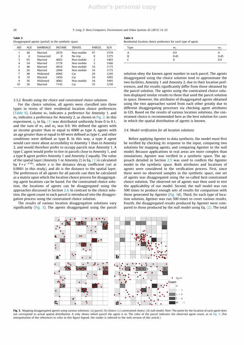
3.3.2. Results using the choice and constrained choice solutionsFor the choice solution, all agents were classified into three

types in terms of their residential location choice preferences(Table 6). Column w1 indicates a preference for Amenity 1, andw2 indicates a preference for Amenity 2, as shown in Fig. 2. In thisexperiment, rij in Eq. (1) was distributed uniformly from 0 to 0.1,and the sum of w1 and w2 was 0.9. We defined the agents withan income greater than or equal to 6000 as type A, agents withan age greater than or equal to 60 were defined as type C, and otherconditions were defined as type B. In this way, a type A agentwould care more about accessibility to Amenity 1 than to Amenity2, and would therefore prefer to occupy parcels near Amenity 1. Atype C agent would prefer to live in parcels close to Amenity 1, anda type B agent prefers Amenity 1 and Amenity 2 equally. The valueof the spatial layer (Amenity 1 or Amenity 2) in Eq. (1) is calculatedby F = e�a*dis, where a is the distance decay coefficient (set at0.0001 in this study), and dis is the distance to the spatial layer.The preferences of all agents for all parcels can then be calculatedas a matrix upon which the location choice process for disaggregat-ing agent locations can be based. For the constrained choice solu-tion, the locations of agents can be disaggregated using theapproaches discussed in Section 2.4. In contrast to the choice solu-tion, the agent count in each parcel is introduced into the disaggre-gation process using the constrained choice solution.

The results of various location disaggregation solutions varysignificantly (Fig. 3). The agents disaggregated using the parcel

solution obey the known agent number in each parcel. The agentsdisaggregated using the choice solution tend to approximate thetwo facilities, Amenity 1 and Amenity 2, due to their location pref-erences, and the results significantly differ from those obtained bythe parcel solution. The agents using the constrained choice solu-tion displayed similar results to those that used the parcel solutionin space. However, the attributes of disaggregated agents obtainedusing the two approaches varied from each other greatly due todifferent disaggregating processes via checking agent attributesin GIS. Based on the results of various location solutions, the con-strained choice is recommended here as the best solution for casesin which the spatial distribution of agents is known.

3.4. Model verification for all location solutions

Before applying Agenter to data synthesis, the model must firstbe verified by checking its response to the input, comparing twosolutions for mapping agents, and comparing Agenter to the nullmodel. Because applications in real areas are more complex thansimulations, Agenter was verified in a synthetic space. The ap-proach detailed in Section 2.5 was used to confirm the Agentermodel in the synthetic space. Both attributes and locations ofagents were considered in the verification process. First, sincethere were no observed samples in the synthetic space, one setof agents was disaggregated using the so-called best-constrainedchoice solution. The observed set of agents was then used to testthe applicability of our model. Second, the null model was run500 times to produce enough sets of results for comparison withthose generated by Agenter (Fig. 3d). Third, for each type of loca-tion solution, Agenter was run 500 times to cover various results.Fourth, the disaggregated results produced by Agenter were com-pared to those produced by the null model using Eq. (2). The total

Table 5Disaggregated agents (partial) in the synthetic space.

AID AGE MARRIAGE INCOME TRAVEL PARCEL SCH

1 46 Married 2679 Non-mobile 97 15782 4 Unmarried 0 No trip 0 13753 65 Married 4663 Non-mobile 2 14634 54 Married 5778 Non-mobile 3 15665 48 Married 4016 Non-mobile 16 11756 26 Married 2904 Non-mobile 16 11757 48 Widowed 6066 Car 29 12458 19 Married 3450 Car 34 10959 56 Widowed 4082 Non-mobile 34 1095

10 26 Married 7143 Car 35 1230

Fig. 3. Mapping disaggregated agents using various solutions: (a) parcel; (b) choice; (c) constrained choice; (d) null model. Note: The point for the location of each agent doesnot correspond to actual spatial distribution. It only shows which parcel the agent is in. The color of the parcel indicates the observed agent count, as in Fig. 2. (Forinterpretation of the references to color in this figure legend, the reader is referred to the web version of this article.)

Table 6Residential location choice preference for each type of agent.

Type w1 w2

A 0.9 0B 0.45 0.45C 0 0.9



number of agents (I) was 100. Three continuous attributes (age, in-come, and SCH) and three categorical attributes (marriage, travel,and parcel) were counted in this process (U + V = 6).

The verification results plotted in Fig. 4 showed that the similar-ity indexes (ranging from 40% to 80%) of the Agenter and the nullmodel did not vary greatly, indicating that both models are stableand the disaggregated agents are repeatable. Agenter produced asignificantly greater SI than the null model, with an average valueof 43.9% (SD = 1.44%), demonstrating that Agenter is better suitedfor disaggregating agents. The better similarity index was assumedto be a result of known information being input into Agenter.Among the three location solutions, the constrained choice solu-tion generated the greatest average SI of 78.5%, which was slightlygreater than the SI of 76.7% observed for the parcel solution. TheSIs of the choice solution were significantly lower than those ofthe constrained choice and parcel solutions, which was likely be-cause the different patterns of agents disaggregated using differentmodels increased the dissimilarities between the spatial locationparcel and the spatial-aware attribute SCH. Overall, the results ofthis test suggested that the constrained choice solution is bestamong the three since the information introduced into Agenterwas the richest.

4. Experiment in the Beijing Metropolitan Area

4.1. Input data

After the Agenter model was applied to the synthetic space, itwas applied to the Beijing Metropolitan Area (BMA) to disaggre-gate heterogeneous residential agents. In this real-space experi-ment, Agenter’s applicability for disaggregating residential agentswas demonstrated using the Fifth Population Census Report ofthe BMA conducted in 2000 (the census), described in the BeijingFifth Population Census Office and Beijing Municipal Statistical Bu-reau (2002), and the Household Travel Survey of Beijing conductedin 2005 (the survey). The census was conducted at the census tractlevel,3 which is similar to the scale of a city block, each of which con-tains dozens of parcels in Beijing. Published census data were aggre-gated from the original census tract level to the district level (18districts in the BMA). The total population count in the censuswas 13.819 million in the BMA.4 The census data provided boththe distributions and relationships among residents. Many

cross-tabulations for various combinations of attributes are listedin this census report, and were used to obtain frequencies and buildrelationships as in Table 3.

The survey covers the entire BMA, including all 18 districtswith 1118 Traffic Analysis Zones (TAZs) as the basic geographi-cal survey unit (Beijing Municipal Commission of Transport andBeijing Transportation Research Center, 2007). The sample sizewas 81,760 households, housing a total of 208,290 persons.There was a 1.36% sampling ratio in contrast to the total popu-lation recorded in the census. The survey provided householdinformation, including household size, hukou status (official res-idence registration),5 residential location at the TAZ level, andpersonal information, including gender, age, household role andjob type and location . The aforementioned information was usedto further validate Agenter in the BMA. In addition, this surveyincluded a one-day travel diary of all respondents, collectedthrough face-to-face interviews. For each trip, the survey recordedthe departure time and location, arrival time and location, trippurpose, mode of transit (both public and individual transporta-tion), trip distance, type of destination building and transit routenumber.

In this experiment, the number of agents to be disaggregatedwas the same as the total number of residents recorded in thecensus (13.819 million). The attributes and locations of residen-tial agents to be disaggregated within the BMA are listed inTable 7. The dependent relationships among attributes are illus-trated in Fig. 5. To save space, all input information regardingdistributions and relationships was stored online as Supplemen-tal material for this paper. The format of the model inputs forthe BMA experiment is the same as that in the synthetic space(Section 3.2 Input data).

The attribute PARCEL is the ID of the parcel used to map thedisaggregated residents. All input rules are available online as ta-bles in an MS Access file. Only typical tables are shown here. Todisaggregate locations of the residential agents, the parcel GISlayer must contain agents for Agenter. The residential parcels(Fig. 6) were extracted from a land use map of the BMA from2000, which has 133,503 polygon parcels, including 26,770 resi-dential parcels. For each residential parcel, the floor area was ob-tained from aggregating buildings within each parcel. Thenumber of residents in each parcel was allocated from each dis-trict available in the census report based on the floor area ofeach parcel, assuming homogeneity in residential floor areas inBeijing. This information is stored as frequencies of the attributeparcels.

Fig. 4. Comparison of disaggregated results generated using the Agenter model and the null model.

3 The spatial distribution of census tracts has never been released from the BeijingMunicipal Statistical Bureau. Therefore, it is not possible to determine whether censustracts are compatible with TAZs.

4 Both registered (with hukou) and unregistered residents (without hukou) wereincluded. 5 Both registered and unregistered residents were interviewed.



4.2. Disaggregating residential agents in the BMA

The disaggregated residential agents (partially listed in Table 8)are mapped in Fig. 7, and are stored as the point Feature Class inthe ESRI Personal Geodatabase. This dataset embeds both the attri-butes and location information of residential agents, which can be

regarded as a primary dataset for urban studies and initializingagent-based models. The disaggregated residential agents and par-cels took up 2.9 GB; the model requires less than 1 h to accomplishthe disaggregation of 1 million residential agents (every agent has10 attributes) for the experiment in the BMA. The test was con-ducted using a workstation with a CPU of 3.0 GHz * 2 and memoryof 4 GB. The amount of time consumed by Agenter primarily de-pends on the number of agents, their attributes, the distribution,and the complexity of the relationship.

5. Discussion

5.1. Validation using the 2005 travel survey

We validated the Agenter model in the BMA using agents ob-served in the survey. In the survey, household and personal infor-mation such as age, sex, income, and number of family memberswere also included. TAM can be calculated based on the TAZlocation (the centroid of each TAZ is used here) for this survey.For a better comparative validation, 208,291 individuals were

Table 7Descriptions and known information for each attribute of residential agents in the BMA.

Name Description Type Known information Data source Data type Order

AGE Age in years Non-spatialattribute

Frequencies The census Ratio 1

SEX Gender Non-spatialattribute

Frequencies The census Nominal (male, female) 2

MARRIAGE Marital status Non-spatialattribute

Frequencies, RB (withAGE)

The census Nominal (married, unmarried, divorced,remarried, widowed)

3

EDUCATION Level of education Non-spatialattribute

Frequencies, RB (withAGE)

The census Ordinal (junior middle school, undergraduate,etc.)

4

JOB Occupation Non-spatialattribute

Frequencies, RB (withEDUCATION)

The census Nominal 5

INCOME Monthly income Non-spatialattribute

Frequencies The survey Ratio 6

FAMILYN Number of family members Non-spatialattribute

Frequencies The census Ordinal (one person, two person, etc.) 7

PARCEL ID of parcel at which theagent resides

Location Frequencies An empiricalstudy

Nominal 8

TAM Distance to the city center Spatialattribute

Location of TiananmenSquare

Urban GIS Ratio 9

Fig. 5. Dependent relationships among attributes of residential agents.

Fig. 6. Residential parcels in the BMA.



disaggregated using Agenter. Input information is given in Sec-tion 4.1. The parcel solution was adopted in Agenter. For compar-ison with the null model, both the Agenter and null models wererun 500 times. In the disaggregated results, the attribute PARCELwas further aggregated into TAZ so the validation could be com-pared to that in a TAZ-scale survey. A total of six attributes wereevaluated for calculation of SI. These were AGE, SEX, INCOME,FAMILYN, TAM, and TAZ. The similarity indicator SI was calculatedusing simulated results and observed results, as shown in Fig. 8.

The average SI of Agenter is 72.6%, which is significantly greaterthan that of the null model (43.9%), indicating that Agenter gener-ates sounder disaggregated agents. Because the null model repre-sents a random disaggregation process, the rules adopted inAgenter regarding the forms of distributions and relationshipsare part of why the present model outperforms the null model.As more comprehensive rules are entered into Agenter, itsperformance in terms of precision may increase further. As shownin Fig. 8, Agenter’s behavior is stable in terms of SI. This demon-strates that Agenter can be used to reproduce individuals in actual

situations, which means representative disaggregated agents canbe retrieved by running Agenter a few times or even only once.

For more solid validation, we also broke down the average SI72.6% for all TAZ and attributes across space and attributes. First,the average SI for each TAZ was calculated based on existing globalresults of 500 simulations. Those TAZs with more samples in andaround the central part of the city were found to have greaterSIs, indicating that more samples lead to better-disaggregated re-sults. This was reasonable considering that the disaggregated re-sults did not closely match the original samples. When a TAZ hasonly 10 or 20 samples, the results become less likely to match. Sec-ond, the SI was calculated based on the sorted disaggregated re-sults and observed samples, as described in Section 2.5. Locationwas given the highest sorting priority, followed by other attributes.Under these conditions, the location of disaggregated results wasthe most consistent with observed samples. The lowest priorityattributes showed the least consistency. For this reason, the attri-bute of interest should be given higher sorting priority. This mayproduce more consistent results.

5.2. Discussion on the experiment results in the BMA

All of the residents were successfully disaggregated in terms ofspatial distribution and socioeconomic attributes in Beijing. This isthe first time that the researchers and planners of the Beijing Insti-tute of City Planning have been able to access large-scale disaggre-gated micro-data regarding the city of Beijing. Agenter wasevaluated and found to be a convenient tool with explicit embed-ded algorithms, and its users are able to easily understand the dis-aggregation mechanism. The disaggregation results in Beijing wereapplied to several small-scale detailed plans for new towns in theBeijing area for the Beijing Affordable Housing Plan. The disaggre-gated population was found to be effective in supporting small-scale plans and policy evaluations, which required fine-scaleindividual data. Before Agenter, these applications were not possi-ble in Beijing, where the municipal governments do not releaseindividual datasets used for census reports or yearbooks. Theextensive applications of this disaggregated population in theBMA are expected in the near future. The travel survey wasconducted in 2005 and the census in 2000, and there were demo-graphic changes in Beijing from 2000 to 2005. Unfortunately, theBeijing travel survey conducted in 2000 was not accessible. Ifaccess becomes available in the near future, the travel surveyin 2010 and the population census of 2010 may be used to update

Table 8Disaggregated residential agents (partial) in the BMA.

AID AGE SEX MARRIAGE EDUCATION JOB INCOME FAMILYN PARCEL TAM

193392 36 Male Married Junior High/MiddleSchool

Production, Transport Equipment Operator, andRelated

2385 Threepersons

888 2140

198316 41 Female Married High School Production, Transport Equipment Operator, andRelated

5966 Threepersons

966 7747

37094 61 Male Married High School Professional Technology Employee 4744 Threepersons

523 5721

165014 27 Male Unmarried High School Business and Service Employees 5559 Five persons 768 49572 41 Female Married Elementary School Production, Transport Equipment Operator and

Related5351 Three

persons18 36739

49808 21 Male Unmarried Junior High/MiddleSchool

Business and Service Employees 2684 Five persons 274 2905

189128 21 Male Married Junior High/MiddleSchool

Production, Transport Equipment Operator andRelated

2578 One person 878 4092

118806 8 Male Unmarried Elementary School Production, Transport Equipment Operator andRelated

0 Threepersons

478 6949

33570 53 Female Married Elementary School Production, Transport Equipment Operator andRelated

1304 Five persons 929 23,760

179469 50 Male Married Elementary School Farming, Forestry, Animal Husbandry and Fishery 4978 Two persons 804 2286

Fig. 7. Spatial distribution of disaggregated agents in the BMA (partial).



the Agenter application in Beijing and disaggregate the 2010population.

There is poor data availability within Beijing, as in most parts ofChina. Exploring the disaggregation of intensive datasets usingknown information provides an opportunity for micro-level simu-lation and analysis through agent-based models (ABMs). Crookset al. demonstrated that ABMs focus on individual objects or cate-gories, and thus disaggregate data are an essential determinant oftheir applicability (2008). Those areas for which there are insuffi-cient micro-level data have a greater chance to develop their ABMsto simulate regional and urban dynamics supported by this ap-proach. The approach proposed here incorporates known dataand information to the greatest degree possible to initialize ABMs.This approach also sheds light on linking macro-datasets andintensive micro-datasets via disaggregation. In addition to initializ-ing ABMs, this approach can be used in the construction of spatialpopulation databases, which are essential to geographers and plan-ners. The approach used herein can generate both population dis-tributions and socio-economic attributes of the population in theform of a spatial population layer that is a key to an urban cyberinfrastructure.

5.3. Limitations of the approach

There are currently several limitations to the Agenter approach.One is that its application can be constrained by the specific datarequirements and assumptions of the approach itself. Specifically,the use of Agenter requires several steps. First, users must selectthe attributes to be disaggregated for agents based on the goalsof the disaggregation. Second, the disaggregation order of attri-butes must be decided based on the dependent relationshipsamong the attributes and the availability of existing information.Third, users must prepare the model input in terms of distributionsand relationships as specified in this study by referring to theexample provided in the online attachment. The online exampleis expected to solve this limitation to some degree. Regarding thesecond limitation, the agents disaggregated by our approach arenot an exclusive set, even though they obey the same existing sta-tistical characteristics of samples. When the disaggregated agentsare used in an ABM, the user is expected to disaggregate numericsets of agents via running Agenter repeatedly using the same input,run the ABM with each set, and then treat the mean value (or otherstatistical characteristics) of the results from all simulations as thefinal simulation result in order to reduce the uncertainty associ-ated with applying this approach to ABMs. Because many combina-tions of micro-agents are generated, this process may eliminateissues associated with the ecological fallacy, a logical fallacy in

the interpretation of statistical data in which inferences regardingthe nature of individuals are deduced from inferences for the groupto which those individuals belong. The ABM does not require anexact reconstruction of the surveyed population’s original spatialdistribution. Rather, it only needs an inferred distribution thatapproximates the actual distribution for purposes of reproducingsimilar patterns and interactions such as those found in the actualdata. Based on this consideration, the model is acceptable for ini-tializing ABMs, despite these limitations.

6. Conclusions

The Agenter approach is proposed in this paper as a means ofdisaggregating heterogeneous agent attributes and locations usingknown information, including aggregate data, small-scale surveys,and empirical studies. The agents to be disaggregated include non-spatial attributes, spatial locations, and spatial attributes. Theknown information is modeled as the distribution of an attributeand as relationships among attributes for disaggregation.

The Agenter model was developed based on the approach pro-posed here. It was used to disaggregate agents in a synthetic spaceand in the BMA. In the first of these experiments, several attributeswere disaggregated using various types of known information, andthen three types of location disaggregation solutions, includingparcel, choice, and constrained choice, were tested. Agenter wasverified using a similarity index (SI) to evaluate the similarities be-tween the disaggregated and observed agents. Agenter producedsignificantly better disaggregation results than the null model(randomly disaggregated) in terms of SI. In the BMA experiment,the Fifth Population Census Report of Beijing in 2000, the House-hold Travel Survey of Beijing in 2005, an empirical study, and theBeijing urban GIS database were all used to infer frequencies ofattributes and relationships among attributes for the disaggrega-tion of all residential agents within the BMA. In this experiment,Agenter was further validated using micro-samples from the sur-vey, and the average SI was found to be 72.6%. These findings indi-cate that Agenter can be applied in the real world to reproduceindividuals that can then be fed into ABMs. Overall, this approachis appropriate to disaggregating agents in situations for whichthere are no micro-data from large-scale surveys. Specifically, themethod developed here can make full use of existing statisticalinformation, surveys, and empirical studies to disaggregate theattribute values and location of agents.

Even though this approach is best suited to preliminary explo-ration, it may solve the bottleneck problems associated with ABMs,like those caused by data scarcity in developing countries. Because

Fig. 8. Validation results of the BMA experiment and comparison with the null model.



all spatially aggregated data are subject to the modifiable areal unitproblem (MAUP), the disaggregated results may allow the user toavoid the MAUP, which occurs because the correlation betweenthe variables in the aggregated data depends on the extent of theareal units used in the aggregation (Openshaw, 1984; Rees, Martin,& Williamson, 2002). Generally, there are few attributes recordedin samples, and unrecorded attributes can be disaggregated usingthis approach. The present approach could supplement conven-tional approaches and may be combined with traditional ap-proaches. Studies on disaggregating Beijing populations withmore attributes by incorporating Agenter and PopGen areunderway.

Acknowledgments

We thank the National Natural Science Foundation of China(No. 51078213) for providing financial support. We also thankthree anonymous reviewers for their valuable comments on ourearlier manuscript.

Appendix A. Supplementary material

Supplementary data associated with this article can be found, inthe online version, at http://dx.doi.org/10.1016/j.compenvurbsys.2013.09.002.

References

A’Hearn, B., Peracchi, F., & Vecchi, G. (2009). Height and the normal distribution:Evidence from Italian military data. Demography, 46, 1–25.

Barthelemy, J, & Toint, P. L. (2013). Synthetic population generation without asample. Transportation Science, 47, 266–279.

Beijing Fifth Population Census Office, & Beijing Municipal Statistical Bureau (2002).Beijing population census of 2000. Beijing: Chinese Statistic Press.

Beijing Municipal Commission of Transport, & Beijing Transportation ResearchCenter (2007). Beijing household travel survey of 2005. Beijing: Internal report.

Benenson, I., Omer, I., & Hatna, E. (2002). Entity-based modeling of urban residentialdynamics: The case of Yaffo, Tel Aviv. Environment and Planning B: Planning andDesign, 29, 491–512.

Birkin, M., & Clarke, M. (1988). SYNTHESIS – A synthetic spatial information systemfor urban and regional analysis: Methods and explanations. Environment andPlanning A, 20, 1645–1671.

Birkin, M., Turner, A., & Wu, B. (2006). A synthetic demographic model of the UKpopulation: Methods, progress and problems. In Proceedings of the secondinternational conference on e-social science. National Centre for ESocial Science,Manchester. <http://www.ncess.ac.uk/events/conference/2006/papers> Accessed15.01.01.

Crooks, A. (2006). Exploring cities using agent-based models and GIS. CASA workingpaper, No. 109. Centre for Advanced Spatial Analysis, University College London,London.

Crooks, A. (2008). Constructing and implementing an agent-based model ofresidential segregation through vector GIS. CASA working paper, No. 133.Centre for Advanced Spatial Analysis, University College London, London.

Crooks, A., Castle, C., & Batty, M. (2008). Key challenges in agent-based modeling forgeo-spatial simulation. Computers, Environment and Urban Systems, 32, 417–430.

Deming, W. E., & Stephan, F. F. (1940). On least squares adjustment of a sampledfrequency table when the expected marginal totals are known. Annals ofMathematical Statistics, 11, 427–444.

Eubank, S., Guclu, H., Anil Kumar, V., Marathe, M. V., Srinivasan, A., Toroczkai, Z.,et al. (2004). Modelling disease outbreaks in realistic urban social networks.Nature, 429, 180–184.

Fienberg, S. E. (1977). The analysis of cross-classified categorical data. Cambridge, MA:The MIT Press.

Hermes, K., & Poulsen, M. (2012). A review of current methods to generate syntheticspatial microdata using reweighting and future directions. Computers,Environment and Urban Systems, 36(4), 281–290.

Holm, E., Lindgren, U., Makila, K., & Malmberg, G. (1996). Simulating an entirenation. In G.P. Clarke (Eds.), Microsimulation for urban and regional policy analysis(pp. 164–186). Pion, London.

Langford, M., & Unwin, D. J. (1994). Generating and mapping population densitysurfaces within a geographical information system. The Cartographic Journal, 31,21–26.

Li, X., & Liu, X. (2007). Defining agents’ behaviors to simulate complex residentialdevelopment using multicriteria evaluation. Journal of EnvironmentalManagement, 85, 1063–1075.

Li, X., & Liu, X. (2008). Embedding sustainable development strategies in agent-based models for use as a planning tool. International Journal of GeographicalInformation Science, 22, 21–45.

Liao, Y., Wang, J., Meng, B., & Li, X. (2010). Integration of GP and GA for mappingpopulation distribution. International Journal of Geographical Information Science,24, 47–67.

Mennis, J. (2003). Generating surface models of population using dasymetricmapping. The Professional Geographer, 55, 31–42.

Müller, K., & Axhausen, K. W. (2010). Population synthesis for microsimulation:State of the art. In Proceedings of the 10th Swiss Transport research conference.<http://e-collection.library.ethz.ch/view/eth:1623?q=microsimulation>Accessed 15.01.12.

Norman, P. (1999). Putting iterative proportional fitting on the researcher’s desk.Working paper 99/03. School of Geography, University of Leeds, UK.

Openshaw, S. (1984). Ecological fallacies and the analysis of areal census data.Environment and Planning A, 16, 17–31.

Pagliara, F., & Wilson, A. (2010). The state-of-the-art in building residential locationmodels. In F. Pagliara et al. (Eds.), Residential location choice: Models andapplications. Advance in spatial science. Berlin, Heidelberg: Springer-Verlag.

Rees, P. (1994). Estimating and projecting the population of urban communities.Environment and Planning A, 26, 1671–1697.

Rees, P., Martin, D., & Williamson, P. (Eds.). (2002). The census data system. London:Wiley.

Robinson, D. T., & Brown, D. (2009). Evaluating the effects of land-use developmentpolicies on ex-urban forest cover: An integrated agent-based GIS approach.International Journal of Geographical Information Science, 23, 1211–1232.

Ryan, J., Maoh, H., & Kanaroglou, P. (2009). Population synthesis: Comparing themajor techniques using a small, complete population of firms. GeographicalAnalysis, 41, 181–203.

Shen, Z., Yao, X., Kawakami, M., & Koujin, M. (2009). Simulating the impact ondowntown of large-scale shopping centre location: Integrating GIS dataset andMAS platform as a case study in Kanazawa city in Japan. In Proceedings of the11th international conference on computers in urban planning and urbanmanagement.

Smith, D. M., Clarke, G. P., & Harland, K. (2009). Improving the synthetic datageneration process in spatial microsimulation models. Environment andPlanning A, 41, 1251–1268.

Stevens, S. S. (1946). On the theory of scales of measurement. Science, 103(2684),677–680.

Wong, D. W. S. (1992). The reliability of using the iterative proportional fittingprocedure. The Professional Geographer, 44, 340–348.

Wu, B. M., Birkin, M. H., & Rees, P. H. (2008). A spatial microsimulation model withstudent agents. Computers, Environment and Urban Systems, 32, 440–453.


author's personal copy · the transims population synthesizer uses ipf for the generation of...

Documents