AUTO - CALIBRATION

Auto- (self-) calibration computes the metric (including internalcamera properties) from multiple projective, uncalibrated images.Camera moves rigidly, absolute conic is fixed, metric geometry can be computed.

Depending on what constraints are given, we need less or moreimages to eliminate the projective ambiguity: projective reconstruction determine a rectifying 4x4 homography H to have the metric reconstruction. -- algebraic structure of the autocalibration problem; -- the absolute dual quadric over many view;-- the Kruppa equations from view pairs;-- the stratified solution, first affine followed by metric;-- special configurations: camera rotating about its center, motion of a stereo rig, camera undergoing planar motion.

Topics:

Algebraic frameworkGiven m cameras, we want to determine in a Euclidean worldframe where a common H (4x4) is to be find. World center, first camera. R^1 = I; t^1 = 0.

k neq 0; take scale of H one; non-singular; based on the first camera.The vector v and 3x3 matrix K^1 specifies the plane at infinity

First calibration matr., upper-triangular, K=K^1 matrix.Conversely, if the first camera is known, thetransformation H coverts projective to metric.

Has to determine 3+5=8 (p + K^1) parameters for H, which isequivalent with plane at infinity (3) and absolute conic (5).All the cameras the projective reconstruction

dual image absolute conic image absolute conic

Relate the unknown omega-s, i=1,...,m, and p, to known A^i, a^i.Example. Same internal parameters.

Each i=2,...,m has max. 5 constraints since KK^T is symmetric. If constraints independent for each view, 5(m-1) >= 8, m>=3. Three views is enough.

multiplies P^i with Hfirst part gives

Absolute dual quadric calibrationDegenerate rank 3, symmetric, positive semi-definite 4x4 matrix encoding both the plane at infinity and the absolute conic.

a framework for auto-calibration

plane at infinity = null vector

determine H, ...or directly from the images

The positive definiteness of omega* some time is not satisfied!Impossing positive semi-definiteness Q*_inf may be not givinga successful solution.

From projective to Euclidean a 3D point is multiplied by H^{-1}

since the cameras are multiplied by H.

obtaining again the

auto-calibration result

plane at infinity = null vector

Linear constraints on if the principal point is known...

...origin then can be in the principal point.

how manyin m views

i vs. j

DIAC has 10 unknowns (4x4 symmetric) scale, det=0 => 8 unk.Example: The principal point known => two equations/view.Four images is enough if the determinant Gives up to four solutions.

Example:Linear solution for only variable focal length. Than: principal point is knows; aspect ratio is unity; skew is zero.From the above table, the linear solution has four equation in eachview. Two views are enough if you have up to four solutions (det=0). Three, or more views have a unique linear solution, because then determinant is equal to zero automatically.

Non-linear (quadratic) type relations in Constant internal parameters.

Five equations between i and j. The , dual absolute quadrichas 8 unknowns. (scale, det=0)Three view enough => ten equations: views 2/1 and views 3/1. Zero skew. One quadratic constraint per view. Also haveThe 8 unknowns can be computed from 8 views.

Symmetric, positive semi-definite matrix eight parameters.

Estimate with algebraic distance iteratively E

unit Frobenius norm. Example. Focal length only. (f^i) m + 3 (p) The determinant is zero automatically from Q*inf

Good initial estimates followed by bundle adjustment. Example: under constant camera parameters and known principal point

Scale factor eliminated by matrix norm. Both terms nomalized to have

next slide

Number of parameters to perform calibration: 8 from m views; k internal parameters known; f fixed but unknown, k + f <= 5. mk + (m-1)f >= 8 gives m ==> how many viewsexample: 2.m + 0.(m-1) >=8 thus m=4

four solutions

Kruppa equationsGerman, around 1910. First auto-calibration in computer vision Faugeras, Luong, Maybank 1992. Two-view constraints, with F known.

algebraic representation of the correspondence of epipolar lines tangent to a conic

[u3]x U = [ [u3]x u1 ... 0] = [u2 -u1 0]

the cross-product eliminatesthe scale between the left and right terms

Example. Focal length for a view pairZero skew. Known principal points, aspect ratio.

Cross-multiplying gives quadraticequations in the two squared unknowns.After solving it, take the square roots.

K is the same. Each view give 2 constraints for the 5 parameters. Those 3 view are enough with F being known. Because are quadratic relations, there are 2^5 solutions! If no rotation F=[e']x the Kruppa equations will not work with the same K.

The statified solution should be used because it puts stronger conditions on the images.

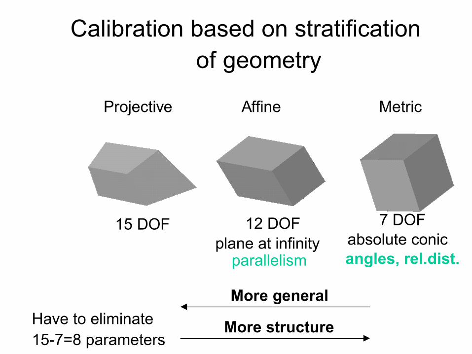
Calibration based on stratification of geometry

15 DOF 12 DOFplane at infinity

parallelism

More general

More structure

Projective Affine Metric

7 DOFabsolute conicangles, rel.dist.

Have to eliminate15-7=8 parameters

the Stratified reconstruction

• up grade reconstruction from perspective to affine[by measuring the plane at infinity]

Recovering the metric reconstruction

•up grade reconstruction from affine to metric[by measuring the absolute conic]

Affine reconstruction - determiningFinding p directly from modulus constraint on plane at infinity.The internal parameters are constant K^i = K, ==> scale factor mu isincluded, the superscripts on R, A, a are not included (a view)

eliminate

infinite homography

-- p appears rank-1 in ap^T, linear terms in the f1,2,3. The relationis a quartic polynomial in p1,2,3. In each view are 4 solutions.-- 3 views (intersection 3 quartic) determines p. Has 4^3 solutions!==>Additional scene information has to be taken into account.Exmp. a vanishing line (two vanishing points) available in twoviews, becomes a one-parameter ambiguity. Applying the modulus constraint results in one quartic equation, max. 4 sol. Finding the plane at infinity is hard in auto-calibration.Three vanishing point correspondence in two views gives the plane . Also: three distant correspondences, notvanishing points!, in the scene give ~plane at infinity. Pure translation between two views determines uniquely theplane at infinity. Three pairs in 2D, give three points in 3D anddefines the plane at infinity.

Affine to metric - determining Easier step! The infinite homography from view 1 to view i

If the first camera not [I | 0] can be converted.

between first and i-th view

Transformation of DIAC and IAC

Once the infinite homography is known, there is a linear relationbetween the omega-s. K solved by Cholesky decomposition.The scale factor

same internal parameters.

The conic has 6-1=5 unknown elements c.m >= 2 views Ac=0 A(6mx6) determine omega uniquely. (rotations between views at different axes!) Numerical stability is a big problem. Computation of K from is extremely sensitive to accuracy of and thennot always is possible to have a positive-definite matrix.

Sensitivity is reduced if further motions, more omega(*) obtained with several Using IAC is prefered because has more linear constraints then DIAC. e.g. Zero-skew case is much simpler. Reflects better the calibration parameters.

Hard constraints, like square pixels, can be imposed directlyfor a more reliable K by adding Cx=0. The constrained total least squares is done differently!

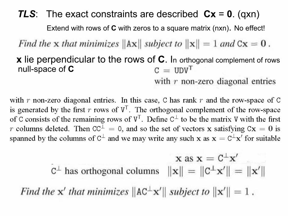
TLS: The exact constraints are described Cx = 0. (qxn) Extend with rows of C with zeros to a square matrix (nxn). No effect!

x lie perpendicular to the rows of C. In orthogonal complement of rows

null-space of C

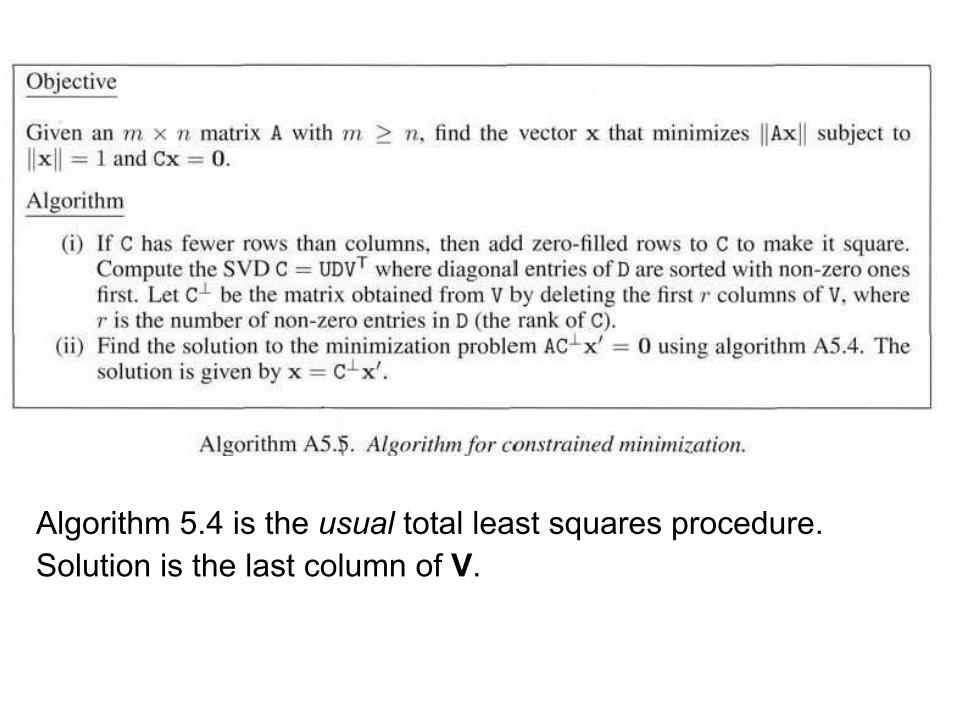
Algorithm 5.4 is the usual total least squares procedure.Solution is the last column of V.

Ambiguities with infinite homographyRotation matrix R has eigenv. direction of rotation From matrix

The point vr is the vanishing point of the rotation axis.

the eigenvector can be obtained

satisfies the relation too! One parameter family. Solutions:

-- Minimum three views, with more than one rotation, different from dr.

-- Internal parameters of the cameras. IAC s=0 add to hard constraint.

[e']x not invertible, Hinf cannot be derived from Kruppa equations.

Typical ambiguities.K has four unknownparametrics

These ambiguities apply to complete sequences. The problem of ambiguity is intrinsic to the motion, and not to any particular auto-calibration algorithm.e.g. one-parameter ambiguity parallel to the rotation axis in the metric reconstruction and a corresponding one-parameter ambiguity in the internal parameters.

Rotating camera calibration

non-translating cameraimpossible to resolvedepth, but metric is stillpossible

Klinear andKiterative areare very close.

Internal parametersare constant butunknown.

Rotation with varying internal parameterspixels are square: skew = 0, aspect ratio unity.Two linear constraints per view. Focal length, principal points are not fixed.

Focal length, principal point quasi constant.pan angle -- horizontal (0...360) around Z axistilt angle -- vertical (-90...90) around Y axis [ roll angle -- (0...360) around X axis ] hand-held camera!

Auto-calibration from planesIt is not possible to determine the depth of the cameras without having

also two points not on the plane. Solution Triggs(1998).Set of image-to-image homographies, related to the first image, then H^i

are easy to be found. Auto-calibration from planes can be done.* The circular points (absolute conic & plane) are mapped between imagesvia homographies and the calibration matrix K determined from thecircular points of a plane (two equations per view). Assume in the first view image of the circular points (4DOF) were found.In each view are two constraints on omega^i. H^1 = I

Circular points, complex conjugate, 4 parameters + v parameters in K^i

in m views. To solve it with two per view 2m >= v + 4

circular points in first image

The problem often non-linear. Iterative method necessary. Requires homography between planes, not 3D points from given 2D views.Including additional information. e.g. If the vanishing line of the imaged plane can be determined, the imaged circular points lie on the vanishingline, only two parameters to be determined.

Auto-calibration of a stereo rigRelative orientation on the rig unchanged during the motion. Internal para.also unchanged. A single motion determines plane at infinity uniquely.Projective structure X before, X' after the motion. Conjugacy relation. Assume XE and X'E are the Euclidean coordinate. HEP 4x4 from projective to Euclidean. then if HE is the non-singular 4x4 from XE to X'E HP conjugate to a Euclidean transformation with same eigenvalues as HE. If E is eigenvector of HE, corresponding eigenvector of HP is Fixed points of a Euclidean transformation. Rotation about Z-axis + unit translation along Z-axis. 3D screw motion.

Two E1,2 are circular points of planes perpendicular the rotation Z-axis.Two E3,4 (identical) eigenvectors are the direction of rotation axis.A 3D point transformation HE

-- Metric calibration based on stratified algorithm. Parameters remain constant. Single motion the internal parameters of each camera are determined up to the one-parameter family resulting from a single rotation. Ambiguity from a single motion can be removed by additional motions, or additional constraints on the internal calibration. -- Planar motion.Orthogonal motion, translation is orthogonal to rotation axis direction.Space of eigenvectors has the two identical eigenvalues.The plane at infinity has a one-parameter family which cannot be eliminated only if a second orthogonal motion about an axis with a different direction from the first is present.

Auto-calibration is not a foul proof method. Works in right circumstances, but can fail in others. Recommendations:-- Avoid small motions, restricted motions (single axis) which not estimate well the infinite homography. This is not apparent if small fields of view.-- Use maximum additional information. Zero skew alone is not enough. Even if it is not 100% correct, include equation(s) on principal points, aspect ratio, taking with small weights.-- Bundle adjustment should have the internal parameters bounded between limits. e.g. aspect ratio 0.5 to 3. Added as additional equations with small weights. Can gives a big improvement in results by not letting the solution to wandering off. -- Restricted motions more reliable than general motion. e.g. rotation of non-translating camera are much more reliable than general motion. Affine reconstruction from a translational motion is better than general motion.

Will not cover:-- Chap.20: Duality. Interchange of the role of cameras and points.The dual algorithm can be used instead of the projective reconstructionalgorithm. -- Chap.21: Cheirality. Relations for the scene to be in the front. -- Chap.22: Degenerate configurations. Geometric constraints with ambiguities of single or multiple views. How can be avoided.