automated and scalable t-wise test case generation

Automated and Scalable T-wise Test CaseGeneration Strategies for Software Product Lines

Gilles Perrouin1, Sagar Sen2, Jacques Klein3, Benoit Baudry2, Yves le Traon1

1LASSY, University of Luxembourg, Luxembourg {gilles.perrouin,yves.letraon}@uni.lu2Triskell Team, IRISA/INRIA Rennes Bretagne Atlantique,{ssen,bbaudry}@irisa.fr

3ISC Department, CRP Gabriel Lippmann, Luxembourg, [email protected]

Abstract—Software Product Lines (SPL) are difficult to val-idate due to combinatorics induced by variability across theirfeatures. This leads to combinatorial explosion of the numberof derivable products. Exhaustive testing in such a large spaceof products is infeasible. One possible option is to test SPLsby generating test cases that cover all possible T feature in-teractions (T -wise). T -wise dramatically reduces the number oftest products while ensuring reasonable SPL coverage. However,automatic generation of test cases satisfying T -wise using SATsolvers raises two issues. The encoding of SPL models and T -wise criteria into a set of formulas acceptable by the solver andtheir satisfaction which fails when processed “all-at-once”. Wepropose a scalable toolset using Alloy to automatically generatetest cases satisfying T -wise from SPL models. We define strategiesto split T -wise combinations into solvable subsets. We designand compute metrics to evaluate strategies on AspectOPTIMA,a concrete transactional SPL.

Index Terms—Model-based Engineering and Testing, Test Gen-eration, T-wise and pairwise, Software Product Lines, Alloy

I. INTRODUCTION

When a company rapidly derives a wide range of different

products a key-challenge is to ensure correctness and safety

of most of these products (if not all) at a low cost. Software

Product Line [1], [2] (SPL) techniques (and tools) allow

engineering such families of related products. However, they

rarely focus on testing the SPL as a whole. A software

product line is usually modeled with a feature diagram [3],

describing the set of features in the SPL and specifying

the constraints and relationships between these features. For

example, mandatory features as well as mutually exclusive

ones can be described. As a result, from a feature diagram

it is possible to derive products by selecting a set of features

that satisfy all the constraints. The product is a software system

built by composing the software assets that implement each

feature.

Product line testing consists in deriving a set of products and

in testing each product. This raises two major issues: 1) the

explosion in the number possible products; 2) the generation

of test suites for products. The first issue rises from the com-

binatorial growth in the number of products with the number

of features. In realistic cases, the number of possible products

is too large for exhaustive testing. Therefore, the challenge

is to select a relevant subset of products for testing. The

This work was supported by the Luxembourg FNR SETER and SPLIT(FNR+CNRS) projects and by EU FP7 Grant agreement 215483 (S-Cube)

second issue is to generate test inputs for testing each of the

selected product. This can been seen as applying conventional

testing techniques while exploiting the commonalities between

products to reduce the testing effort [4], [5], [6]. Here, we

focus on the first issue: How can we efficiently select a subset

of products for product line testing?

Previous work [7], [8] has identified combinatorial inter-

action testing (CIT) as a relevant approach to reduce the

number of products for testing. CIT is a systematic approach

for sampling large domains of test data. It is based on the

observation that most of the faults are triggered by interactions

between a small numbers of variables. This has led to the

definition of pairwise (or 2-wise) testing. This technique

selects the set of all combinations so that all possible pairs

of variable values are included in the set of test data. Pairwise

testing has been generalized to T -wise testing which samples

the input domain to cover all T -wise combinations. In the

context of SPL testing, this consists of selecting the minimal

set of products in which all T -wise feature interactions occur

at least once.

Current algorithms for automatic generation of T -wise test

data sets have a limited support in the presence of depen-

dencies between variable values. This prevents the application

of these algorithms in the context of software product lines

since feature diagrams define complex dependencies between

variables that cannot be ignored during product derivation.

Previous work [9], [10] proposed to use constraints solvers as a

possibility to deal with this issue. However, they still leave two

open problems: scalability and the need for a formalism to ex-

press feature diagrams. The former is related to the limitations

of constraint solvers when the number of variables and clauses

increases. Above a certain limit, solvers cannot find a solution,

which makes the approach infeasible in practice. The latter

problem is related to the engineering of SPLs. Designers build

feature diagrams using editors for a dedicated formalism. On

the other hand, constraint solvers manipulate clauses, usually

in Boolean Conjunctive Normal Form (CNF). Both formalisms

are radically different in their expressiveness and modeling

intention. This is a major barrier for the generation of T -wise

configurations from feature diagrams.

In this paper, we propose an approach for scalable automatic

generation of T -wise products from a feature diagram. Current

constraint solvers have a limit in the number of clauses they

can solve at once. It is necessary to divide the set of clauses

into solvable subsets. We compose the solutions in the subsets

to obtain a global set. In this work, we investigate two “divide-

and-compose” strategies to divide the problem of T -wise

generation for a feature diagram into several sub problems that

can be solved automatically. The solution to each sub problem

is a set of products that cover some T -wise interactions. The

union of these sets cover all interactions, thus satisfying the

T -wise criterion on the feature diagram. However “divide-and-

compose” strategies may yield a higher number of products to

be tested and redundancy amongst them which is the price for

scalability. We define metrics to compare the quality of these

strategies and apply them on a concrete case study.

Our T-wise testing toolset first transforms a given feature

diagram and its interactions into a set of constraints into

Alloy [11], [12], a formal modeling language, based on first-

order logic, and suited for automatic instance generation.

Then it complements the Alloy model with the definition of

the T -wise criteria and applies one of the chosen strategies

to produce a suite of products forming test cases. Finally,

metrics are computed giving important information on the

quality of the test suite. We extensively applied our toolset

on AspectOPTIMA [13], [14] a concrete aspect-oriented SPL

devoted to transactional management.

The remainder of the paper is structured as follows: Section

II details the context of SPL testing and motivates the problem.

Section III describes the metrics to assess SPL test generation

strategies. Section IV gives an overview of the product gen-

eration approach. In Section V we present two “divide-and-

compose” strategies. In Section VI we present experiments to

qualify our strategies on the AspectOPTIMA SPL. Section

VII presents related contributions in the field and Section VIII

draws some conclusions and outlines future work.

II. CONTEXT AND PROBLEM

A. Context

In this paper, we focus on generating a small set of test

products for a feature diagram. A product is a valid config-

uration of the feature diagram that can be used as a relevant

test case for the SPL. We give a brief definition and example

of feature diagrams before describing test case generation for

such structures.

Feature Diagram: Feature Diagrams (FD) introduced by

Kang et al. [3] compactly represent ( Figure 1) all the

products of an SPL in terms of features 1 which can be

composed. Feature diagrams have been formalized to perform

SPL analysis [15], [16], [17], [18]. In [16], [17], Schobbens et

al. propose an generic formal definition of FD which subsumes

many existing FD dialects. FDs are defined in terms of a

parametric structure whose parameters serve to characterize

each FD notation variant. GT (Graph Type) is a boolean

parameter indicates whether the considered notation is a Direct

Acyclic Graph (DAG) or a tree. NT (Node Type) is the set

of boolean operators available for this FD notation. These

1Defined by Pamela Zave as “An increment in functionality”. See http://www.research.att.com/∼pamela/faq.html

operators are of the form opk with k ∈ N denoting the number

of children nodes on which they apply to. Considered operators

are andk (mandatory nodes), xork (alternative nodes) ork

(true if any of its child nodes is selected), optk (optional

nodes). Finally vp(i..j)k (i ∈ N and j ∈ N ∪ ∗) is true if

at least i and at most j of its k nodes are selected. Existing

other boolean operators can usually be expressed with vp.

GCT (Graphical Constraint Type) is the set of binary boolean

functions that can be expressed graphically. A typical example

is the “requires” between two features. Finally, TCL (Textual

Constraint Language) tells if and how we can specify boolean

constraints amongst nodes. A FD is defined as follows:

• A set of nodes N , which is further decomposed into a

set of primitive nodes P (which have a direct interest

for the product). Other nodes are used for decomposition

purposes. A special root node, r represents the top of the

decomposition,

• A function λ : N �→ NT that labels each node with a

boolean operator,

• A set DE ∈ N ×N of decomposition edges. As FDs are

directed, node n1, n2 ∈ N, (n1, n2) ∈ DE will be noted

n1 → n2 where n1 is the parent and n2 the child,

• A set CE ∈ N ×GCT ×N of constraint edges,

• A set φ ∈ TCL

A FD has also some well-formedness rules to be valid:

only root (r) has no parent; a FD is acyclic; if GT = true

the graph is a tree; the arity of boolean operators must be

respected. We build upon this formalization to create feature

modeling environments supporting product derivation [19]

where we encode the AspectOPTIMA SPL feature diagram (see

figure 1). We implement AspectOPTIMA SPL as an aspect-

oriented framework providing run-time support for different

transaction models. AspectOPTIMA has been proposed in [14],

[13] as an independent case study to evaluate aspect-oriented

software development approaches, in particular aspect-oriented

modeling techniques. Once we defined the FD, we can create

products (i.e a selection of features in the FD). To be valid, a

product follows these rules: 1) The root feature has to be in

the selection, 2) The selection should evaluate to true for all

operators referencing them, 3) All constraints (graphical and

textual) must be satisfied 4) For any feature that is not the root,

its parent(s) have to be in the selection. We enforce the validity

of a product according to well-formedness rules defined on

our generic metamodel [19] which are automatically translated

to Alloy by our FeatureDiagram2Alloy transformation (see

Section IV). Once we introduce the notion of feature diagram

and formalize it we can form our notion of SPL testing on

such an entity.

SPL Test Case: A SPL test case is one valid product (i.e.

a ) of the product line. Once this test case is generated from

a feature diagram, its behaviour has to be tested.

SPL Test Suite: A SPL Test Suite is a set of SPL test cases.

Example: Figure 2 presents 3 test cases, three products

which can be derived from the feature model. These three

test cases form a test suite.

Transaction

Recovering

OptimisticValidation

OutcomeAware

Deferring

Optional feature

Checkpointing

Context

Nested

Tracing

AccessClassified

Traceable

Lockable

Shared

Checkpointable

Copyable

Composition Rule:‘2-PhaseLocking’ excludes ‘Recovering.Deferring’

Composition Rule:‘OptimisticValidation’ requires ‘Recovering.Deferring’

XOR featureKey:

SemanticClassified

Composition Rule:‘Deferring.Traceable’ requires ‘Traceable.SemanticClassified’

PhysicalLogging2-PhaseLocking

ConcurrencyControlStrategy

AND feature

Fig. 1. Feature Diagram of AspectOPTIMA

Product 3:

NestedTransaction

Recovering

OutcomeAware Checkpointing

Context

Tracing

AccessClassifiedTraceable

Lockable

CheckpointableCopyable

PhysicalLogging2-PhaseLocking


Transaction

Recovering OptimisticValidation

OutcomeAware

Deferring

Context

Nested

AccessClassified

TraceableLockable

SharedPhysicalLogging


Product 2:

SemanticClassified

Transaction

Recovering

OutcomeAware Checkpointing

Context

Tracing

AccessClassified

Traceable

LockableCheckpointable

Copyable

PhysicalLogging 2-PhaseLocking


Product 1:

Fig. 2. Three Test Cases

Valid/Invalid T -tuple: A T -tuple ( were T is a natural

integer giving the number of features present in the T -

tuple2) of features is said to be valid (respectively invalid),

if it is possible (respectively impossible) to derive a product

that contains the pair (T -tuple) while satisfying the feature

diagram’s constraints.

Example: In the AspectOptima product line we have a

total of 19 features. All these 19 features can take the

value true or false. Thus, we can generate 681 pairs that

2In general we will use the term “tuple” to mention a T -tuple when t doesnot matter. In the special case of pairwise, i.e. when T = 2, we denote a2-tuple by the term “pair”.

cover all pairwise combinations of feature values. How-

ever, not all of these pairs can be part of a product

derivable from the feature model. For example, the pair

<(not Transaction), Recovering> is invalid with

respect to the AspectOptima feature diagram which specifies

that the feature Transaction is mandatory.

SPL test adequacy criterion: To determine whether a test

suite is able to cover the feature model of the SPL, we need

to express test adequacy conditions. In particular, we consider

the “T-wise” [8], [9] adequacy criterion (all-T -tuples) were

each valid T -tuple of features is required to appear in at least

one test case.

Example: The test suite presented in figure 2 does

not satisfy our adequacy criterion since the pair (2-tuple)

<semantic classified, lockable> does not appear

in any of the three test cases.

Test generation: In our context of SPL testing, test gen-

eration consists of analyzing a feature diagram in order to

generate a test suite that satisfies pairwise coverage.

Pairwise (and more generally T-wise) is a set of constraints

over a range of variables (mathematically defined as coveringarrays [20]). Thus it is possible to use SAT-solving technology

[21], [22], [23] to compute such arrays. In our case, variables

are the features of a given given feature diagram. It is therefore

mandatory to encode a feature diagram in first order logic so

that SAT-solvers can analyze them. Thanks to feature diagram

formalization, this is possible [15], [18] and have been done

for various purposes [24], [25].

B. Problem

The work in this paper builds upon this idea: model the test

generation problem as a set of constraints and ask a constraint

solver for solutions. In this context we tackle two issues:

(1) modelling the SPL test generation problem in order to

use a constraint solver and (2) dealing with the scalability

limitations of SAT solvers. Our contribution on the first issue

is an automatic transformation from a feature diagram to an

Alloy [12] model.

Scalability is a major issue with SAT solvers. It is known

that solving a SAT formula on more than 2 variables is an

NP-complete problem. It is also known that depending on the

number of variables and the number of clauses, satisfiability

or unsatisfiability is more or less computationally complex

[26]. However, we currently don’t know how to predict the

computation complexity of a given problem. An empirical

approach thus consists in trying to solve the set of “constraints

all-at-once”. Three things can happen: the solver returns a

solution, the solver returns an unsatisfiability verdict, the

solver crashes because the problem is too complex. In the

latter case, one way to generate a test suite that covers t-

wise interactions, is to decompose the problem into simpler

problems, solve them independently and merge the solutions.

In the following, we refer to this approach as “divide-and-

compose” approach.

One pragmatic approach, and a naive one, consists of

running the solver once for each T -tuple that has to be covered.

This iterative process is the simplest “divide-and-compose”

approach and it generates one test case for each valid T -

tuple in the FD. For the AspectOPTIMA SPL, we obtain 421

test cases that satisfy pairwise and that corresponds to 421

products to be tested. The all-pairs criterion is satisfied but

with a large number of products. It also has to be noted

that only 128 different products can be instantiated from the

AspectOPTIMA SPL. This indicates that the application of

“divide-and-compose”, although it might define problems that

can be solved, also introduces a large number of redundant

test cases in the resulting test suite. Indeed, if it generates 421

test cases, but there can be only 128 different test cases, there

is an important redundancy rate.

In general, a solution for generating a test suite with a SAT

solver consists in finding a strategy to decompose the SAT

problem in smaller problems that can be automatically solved.

Also, the strategy should decompose the problem in such a

way that when the solutions to all sub-problems are composed,

the amount of redundancy in the suite is limited.

Test generation strategies: In this paper, we call strategiesthe ways we “divide-and-compose”. Depending on applied

strategies and their parameters we will derive more or less

test cases. Before delving into the two different strategies we

will introduce metrics to evaluate them in the next section.

III. METRICS FOR STRATEGY EVALUATION

We need efficiency and quality attributes in order to evaluate

the generated SPL test cases and compare the automatic

generation strategies. The first efficiency attribute relates to

the size of the generated SPL test suite.

SPL Test suite size: The size of a test suite is defined by

the number of SPL test cases that a given generation strategy

computes. In the best case, we want a strategy to generate the

minimal number of test cases to satisfy the SPL test adequacy

criterion. As this optimal number is generally not known a

priori, we use the SPL test suite size as a relative measure to

compare test generation strategies.

A second efficiency attribute relates to the cost of test

generation in itself. We measure this cost as the time taken

for generation.

SPL strategy time taken: We characterize the cost of a given

strategy by the time it took to decompose the problem into

solvable sub-problems and the time it took to merge the partial

generated solutions to a SPL test suite.

We also evaluate the quality of the generated test cases.

First, we want to appreciate the coverage of the generated

test cases with respect to the feature diagram. We measure

coverage by looking at the rate of similarity between the test

cases that are generated. The intuition is that, the more test

cases are similar, the less they cover the variety of products

that can be generated from the feature diagram.

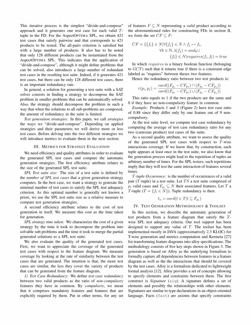
1) Test Case Redundancy: We define test case redundancybetween two valid products as the ratio of non-compulsoryfeatures they have in common. By compulsory, we mean

that it comprises mandatory features and features that are

explicitly required by them. Put in other terms, for any set

of features F ⊆ N representing a valid product according to

the aforementioned rules for constructing FDs in section II,

we form the set CF ⊆ F :

CF = {{fi} ∈ N |∀{fj} ∈ N ∧ fj �→ fi,

∀k ∈ N, λ(fj) = andk∪{fl} ∈ N |requires(fi, fl) = true

In which requires is a binary boolean function (belonging

to GCT ) such that it returns true if there is a constraint edge

labeled as “requires” between theses two features.

Hence the redundancy ratio between two test products is:

r(pi, pj) =card((Fpi

− CFpi) ∩ (Fpj

− CFpj))

card((Fpi− CFpi

) ∪ (Fpj− CFpj

))

This ratio equals to 1 if the two products are the same and

0 if they have no non-compulsory feature in common.

Example: Products 1 and 3 (Figure 2) have test case ratio

of 0.88 since they differ only by one feature out of 9 non-

compulsory.

At the test suite level, we compute test case redundancy by

computing the average of test case redundancy ratio for any

two (cartesian product) test cases of the suite.

As a second quality attribute, we want to assess the quality

of the generated SPL test cases with respect to T -wise

interactions coverage. If we know that, by construction, each

tuple appears at least once in the test suite, we also know that

the generation process might lead to the repetition of tuples an

arbitrary number of times. For the SPL testers, such repetitions

imply that they will test the same interaction of features several

times.

T -tuple Occurrence: is the number of occurrences of a valid

pair (T -tuple) in a test suite. Let TS a test suite comprised of

pi valid cases and Fpi ⊆ N their associated features. Let T a

T -tuple (T = {fi ∈ N}). Tuple redundancy is then:

to = card(t ∈ T |t ⊆ Fpi)

IV. TEST GENERATION METHODOLOGY & TOOLSET

In this section, we describe the automatic generation of

test products from a feature diagram that satisfy the T -

wise SPL test adequacy criteria. Our tool support has been

designed to support any value of T . The toolset has been

implemented mostly in JAVA (approximatively 2.3 KLOC) for

T-wise generation and metrics computation and Kermeta [27]

for transforming feature diagrams into alloy specifications. The

methodology consists of five key steps shown in Figure 3. The

generation is based on Alloy as the underlying formalism to

formally capture all dependencies between features in a feature

diagram as well as the the interactions that should be covered

by the test cases. Alloy is a formalism dedicated to lightweight

formal analysis [12]. Alloy provides a set of concepts allowing

to specify elements and constraints between them. The first

construct is Signature (sig). A signature defines a set of

elements and possibly the relationships with other elements.

Signatures are similar to type declarations in an object-oriented

language. Facts (fact) are axioms that specify constraints

Software Product LineFeature Diagram

1. TransformationFeatureDiagram2Alloy

2. Generation of initial T−wise tuples l

3. Detection of Valid tuples

4. Creating and Solving Conjunctions of Tuples

BinarySplit IncrementalGrowth

5. Analysis

Value of T

Alloy Feature DiagramAF

Set of Valid TuplesV

[Min,Max] Scope[Min,Max] DurationSelection Strategy

Set of Test Cases (Products)covering all Valid Tuples

P

Fig. 3. Product Line Test Generation Methodology

about elements and relationships. These axioms must always

hold, they are close to the concept of invariants in other

specification languages. Predicates, (pred), as opposed to

facts, define constraints which can evaluate to true or false.

With these constructs it is possible to construct various kinds

of Alloy models and to ask alloy if it is possible to find

instances that satisfy all constraints and evaluate one predicate

to true. The scope is an integer bound on the maximum number

of instances for each signature [12]. This allows to limit the

search space in which Alloy looks for a solutions and this is

a way to finely tune how Alloy builds instances satisfying a

model.

A. Step 1: Transforming Feature Diagrams to Alloy

In order to generate valid test products directly from a

feature diagram, we need to transform the diagram in a model

that captures constraints between features (defined in Section

II). The FeatureDiagram2Alloy transformation automatically

generates an Alloy model AF from any feature diagram FDexpressed in our generic feature diagram formalism [19].

s i g T r a n s a c t i o n {}s i g Nes ted {}s i g R e c o v e r i n g {}s i g C o n n c u r r e n c y C o n t r o l S t r a t e g y {}s i g P h y s i c a l L o g g i n g {}s i g TwoPhaseLocking {}s i g O p t i m i s t i c V a l i d a t i o n {}s i g C h e c k p o i n t i n g {}s i g D e f e r r i n g {}s i g OutcomeAware {}s i g C h e c k p o i n t a b l e {}s i g T r a c i n g {}s i g C o n t e x t {}s i g Copyable {}s i g T r a c e a b l e {}s i g Shared {}s i g S e m a n t i c C l a s s i f i e d {}s i g A c c e s s C l a s s i f i e d {}s i g Lockab le {}

Listing 1. Generated Signatures for Features in AspectOptima

The AF model captures all features as Alloy signaturesand a set of Alloy signatures that capture all constraints and

relationships between features. This model also declares two

signatures that are specific to test generation: configurationthat corresponds to a test case and that encapsulates a set of

features (listing 2); ProductConfiguration (listing 3) which will

encapsulate a set of test cases.

Example: In the AspectOptima feature diagram, shown

in Figure 1, we have 19 features f1, f2, ..., f19. The trans-

formation FeatureDiagram2Alloy generates 19 signatures to

represent these features shown in listing 1.

s i g C o n f i g u r a t i o n

{f1 : one T r a n s a c t i o n , / / Mandatory

f2 : l one Nested , / / O p t i o n a l

. . .

f19 : one Lockab le / / Mandatory

}

Listing 2. Generated Signature for Configuration of Features inAspectOptima

one s i g P r o d u c t C o n f i g u r a t i o n s

{c o n f i g u r a t i o n s : s e t C o n f i g u r a t i o n

}

Listing 3. Generated Signature for Set of Configurations

The FeatureDiagram2Alloy transformation generates Alloyfacts in AF .

Example: In the listing 4 we present two generated Alloy

facts showing mutually exclusive (XOR) features selection:

f6 (TwoPhaseLocking) and f7 (OptimisticValidation) given

that f4 (ConcurrencyControlStrategy) has been selected. These

facts must be true for all configurations.

/ / Two Phase Locking XOR O p t i m i s t i c V a l i d a t i o n C o n s t r a i n t 1

pred T w o P h a s e L o c k i n g c o n s t r a i n t

{a l l c : C o n f i g u r a t i o n | # c . f6 ==1 i m p l i e s (# c . f4 =1 and # c . f7 =0)

}

/ / Two Phase Locking XOR O p t i m i s t i c V a l i d a t i o n C o n s t r a i n t 2

pred O p t i m i s t i c V a l i d a t i o n c o n s t r a i n t

{a l l c : C o n f i g u r a t i o n | # c . f7 ==1 i m p l i e s (# c . f4 =1 and # c . f6 =0)

}

Listing 4. Generated Fact for XOR

The FeatureDiagram2Alloy transformation has been imple-

mented as a model transformation in the Kermeta metamod-

eling environement [27]. Since our feature diagram formalism

is generic [19] various kinds of feature diagrams can be

automatically transformed.

B. Step 2: Generation of Tuples

In Step 2, we automatically compute the set I of all possible

tuples from feature diagram AF and the number T . The tuples

enumerate all T -wise interactions between all selections of

features in AF .

Example: The 3-tuple t =< #f1 = 0, #f2 = 1, #f3 =1 > for the value T = 3 contains 3 features and their

valuations. In the tuple we state that the set of test products

must contain at least one test case that has features f2 and f3

and does not have f1.

The initial set of tuples I is the set of tuples that cover all

combinations of T features taken at a time. For example, if

there are N features then the size of I is 2NCT minus all

tuples with repetitions of the same selected feature.

Each tuple t in I also has an Alloy predicate representation.

An Alloy predicate representation of a tuple t is t.predicate.

Example: The tuple t =< #f1 = 0, #f2 = 1, #f3 = 1 >is shown in listing 5.

pred t

{some c : C o n f i g u r a t i o n | # c . f1 =0 and # c . f2 =1 and # c . f3 =1

}

Listing 5. Example Tuple Predicate

C. Step 3: Detection of Valid Tuples

In this third step, we use the predicates derived from each

possible tuple in order to select the valid ones according to

the feature diagram. We say that a tuple is valid if it can be

present in a valid instance of the feature diagram F .

Example: Consider AspectOptima (in Fig-

ure 1) features f1:Transaction, f2:Nested, and

f4:ConcurrencyControlStrategy, The 3-tuple t =< #f1 =0, #f2 = 1, #f4 = 1 > is not a valid tuple as the

feature f4 required the existence of feature f1 and

hence we neglect it. On the other hand, the 3-tuple

t =< #f1 = 1, #f2 = 0, #f4 = 1 > is valid since all

feature selections hold true for F . We determine the validity

of each such tuple t by solving AF ∪ t.predicate for a scope

of exactly 1. This translates to solving the Alloy model to

obtain exactly one product for which the tuple t holds true.

Example: For the AspectOptima case study we generate

681 tuples for pair-wise (T = 2) interactions in the initial set

I . We select 421 valid tuples in the set V .

D. Step 4: Creating and Solving Conjunctions of MultipleTuples

Once we have a set of valid tuples, we can start generating

a test suite according to the T -wise SPL adequacy criteria.

Intuitively, this consists in combining all valid tuples from Vwith respect to AF in order to generate test products that cover

all T-wise interactions.

Example: For pair-wise testing in the case of AspectOptima

this amounts to solving a conjunction of 421 tuple predicates

t1.predicate∩ t2.predicate∩ ...∩ t421.predicate for a certain

scope.

The major issue we tackle in this work is that in general,

constraint solvers cannot generate the conjunction of all valid

tuples at once.

Example: Using the “all-at-once” strategy on

aspectOPTIMA, with 421 valid tuples, the generation

process crashes without giving any solution after several

minutes using MiniSAT [23] solver.

Hence we derived two “divide-and-compose” strategies to

break down the problem of solving a conjunction of tuples

to smaller subsets of conjunction of tuples. The strategies

we present are Binary Split and Incremental Growth. Each

strategy is parameterized by intervals of values defining the

scope of research for each (sub)-conjunction of tuples, the

duration in which Alloy is authorized to solve the conjunction

as well as a strategy defining how features are picked in a

tuple. We describe these strategies in more detail in section

V. The combination of solutions is a test suite TS that covers

all tuples.

1) Step 5: Analysis: In order to assess the suitability of our

“divide-and-compose” strategies and compare their ability to

generate test suites, we need to compute the metrics defined in

section III. We compute for each generated test suite the num-

ber of products or test cases, test case and tuple redundancy.

We performed extensive experimentation on AspectOPTIMA

by generating test suite with different scope and time values.

We present consolidated results of these experiments in section

VI.

V. TWO STRATEGIES FOR T -WISE SPL TEST SUITE

GENERATION

As mentioned previously, to be scalable we divide the prob-

lem of solving tuples into sub-problems, i.e. we are creating

conjunctions of subsets of tuples. We solve the conjunction of

tuples in each of these subsets using the algorithm presented

in Section V-A. The first strategy to obtain subsets of tuples,

Binary Split, is discussed in Section V-B. We present the

second strategy, Incremental Growth, in Section V-C.

A. Solving a Conjunction of Tuples

We solve a conjunction of tuples using the Algorithm

1. We combine the Alloy model AF with a predicate

CT (S).predicate representing the conjunction of tuples in

the set S = t1, t2, ..., tL. We solve the resulting Alloy model

m using incremental scoping. We create a run command cstarting for a scope between the minimum scope mnSc and the

max scope mxScope. We insert the command c into m. A SAT

solver such as MiniSAT [23] or ZChaff [22] is used to solve m.

We determine the duration dur = startT ime− endT ime for

each scope value. If dur exceeds maximum duration mxDurwe stop incrementing the scope. The solve method returns the

result of the SAT solving and the corresponding solution if

a solution exists.

Algorithm 1 solveCT(AF , S,mnSc, mxSc, mxDur) :

Boolean, A4SolutionLet current model m = AF ∪ CT (S).predicatescope← mnScresult← Falsedur ← 0while scope ≤ mxSc ∧ dur ≤ mxDur do

Let c = “run” CT (S).name for < scope >m← m ∪ cstartT ime = currentT imesolution = SATsolve(m)if solution.isEmpty then

result← Falsescope← scope + 1Remove command c from m

if !solution.isEmpty thenresult← TrueBreak While Loop

endT ime← currentT imedur ← endT ime− startT ime

Return {result, solution}

B. Binary Split

The binary split algorithm shown in Algorithm 2 is based

on splitting the set of all valid tuples V into subsets (halves)

until all subsets of tuples are solvable. We first order the

set of valid tuples based on the strategy Str. The strategy

can be random or based on distance measure. In this paper,

we consider a random ordering. The Pool is set of sets of

tuples. Initially, Pool contains the entire set of valid tuples

V . If each set of tuples Pool[i], 0 ≤ i ≤ Pool.size in

Pool is not solvable in the given range of scopes mnSc and

mxSc or within the maximum duration mxDur then result is

False for Pool[i]. A single value of result = False renders

AllResult = False. In such a case, we select the largest set in

Pool[i] and split it into halves {H1} and {H2}. We insert the

halves {H1} and {H2} into Pool[i]. The process is repeated

until all sets of tuples in Pool can be solved given the time

limits and AllResult = True. In the worst case, binary split

convergences with one tuple a set making Pool.size = V.sizeas all tuples in V are solvable.

Algorithm 2 binSplit(AF , V, mnSc,mxSc,mxDur, Str)

AllResult← TrueV ← order(V, Str)Pool← {{V }}repeat

result← Falsei← 0repeat{result, Pool[i].solution}← solve(AF , Pool[i], mnSc, mxSc, mxDur)i← i + 1AllResult← AllResult ∧ result

until i == Pool.sizeif AllResult == False then{L} = max(Pool){{H1}, {H2}} = split({L}, 2)Pool.add({H1})Pool.add({H2})

until AllResult = falseReturn Pool

C. Incremental Growth

The incremental growth is shown in Algorithm 3. In the

algorithm we incrementally build a set of tuples in the con-

junction CT and add it to the Pool. The select function based

on a strategy Str selects a tuple in V and inserts it into

CT . The strategy Str can be random or based on a distancemeasure between tuples. In this paper, we consider only a

random strategy for selection. We select and remove a tuple

from V and add it to CT until the conjunction cannot be

solved anymore ,i.e. result = False. We remove the last

tuple and put it back into V . We include CT into Pool. In

every iteration, we initialize a new conjunction of tuples until

we obtain sets of tuples in Pool that contain all tuples initially

in V or when V is empty.

VI. EXPERIMENTS

The objective for our experiments is: To demonstrate the

feasibility of “divide-and-compose” strategies (Binary Split

and Incremental Growth) and compare their efficiency with

respect to test case generation. All experiments are performed

on a real-life feature model: AspectOPTIMA. In this section

Algorithm 3 incGrow(AF , V, mnScp,mxScp,mxDur, Str)

Pool← {}repeat

CT ← {}repeat

tuple← V.select(Str)CT.add(tuple){result, CT.solution}← solve(AF , CT, mnSc, mxSc, mxDur)if result == False then

CT.remove(tuple)V.add(tuple)

until result == FalsePool.add(CT )

until V.isEmptyReturn Pool

we report and discuss the automatic generation of T-wise test

suites for this model.

A. Experimental Setting

We automatically generate test suites with the two “divide-

and-compose” strategies and compare them according to: (a)

the number of generated test cases; (b) the number of tuple

occurrences in the test suites; (c) the similarity of the products

in the generated test suites. For both strategies we have to set

the values for two parameters that specify the search space:

the scope and the time limit. We vary the scope over 5 values:

3, 4, 5, 6, 7; the maximum duration mxDur to find a solution

for a given conjunction of constraints is fixed at 1600ms. We

generate 100 sets of products for each scope giving us a total of

5×100 sets of products for a strategy. The reason we generate

100 solutions is to study the variability in the solutions given

that we use uniform random ordering in binary split and

random tuple selection in incremental growth. Therefore, for

two strategies we have 2 × 5 × 100 sets of products or test

cases. We perform our experiments on a MacBook Pro 2007

laptop with the Intel Core 2 Duo processor and 2GB of RAM.

Before studying the results of our experiments we note that

attempting “solving-all-constraints-as-once” does not yield any

solutions for the AspectOPTIMA SPL. This is true even

for simple feature models such as AspectOPTIMA that does

not lead to derivation of billions of products (like industrial

product lines). On the other hand, all executions of both

“divide-and-compose” strategies generate T-wise test suites.

This first observation indicates that these strategies enable the

usage of SAT solvers for the automatic generation of T-wise

interactions test suites for both simple and potentially complex

feature models. This is the first main result of our study.

B. Number of Products Vs. Scope

In Figure 4, we present the number of products generated

for different scopes, which corresponds to the number of test

cases in a suite. Each box and its whiskers correspond to

100 solutions generated using a strategy for a given scope.

On the x-axis we have scope for two strategies: BinarySplit

represented by bin scope and IncrementalGrowth represented

by inc scope.

120

BinarySplit Incremental

80

100

120

Upper Quartile (Q3)

max

Upper Whisker


60

80

100

120uc

ts

Upper Quartile (Q3)

max

Upper Whisker

median (Q2)

Lower Whisker

min


40

60

80

100

120er

OfP

rodu

cts

Upper Quartile (Q3)

max

Upper Whisker

median (Q2)

Lower Whisker

min

average

Lower Quartile (Q1)


20

40

60

80

100

120N

umbe

rOfP

rodu

cts

Upper Quartile (Q3)

max

Upper Whisker

median (Q2)

Lower Whisker

min

average

Lower Quartile (Q1)


0

20

40

60

80

100

120N

umbe

rOfP

rodu

cts

Upper Quartile (Q3)

max

Upper Whisker

median (Q2)

Lower Whisker

min

average

Lower Quartile (Q1)


0

20

40

60

80

100

120N

umbe

rOfP

rodu

cts

Upper Quartile (Q3)

max

Upper Whisker

median (Q2)

Lower Whisker

min

average

Lower Quartile (Q1)


Fig. 4. Box Plot for Number of Products vs. Scope

For the binary split strategy, the number of products is high

for a scope of 3 (average of 50 products), decreases towards a

scope of 5 (average 18 products) and increases again towards

a scope of 7 (average of 35 products). In our experiments

the scope nearest to the minimal number of test cases is 5.

For a scope of 7 we ask the solver to create 7 products per

subset of tuples (or pairs) while only 5 products suffice for

the same set of tuples leading to more products that satisfy thesame set of tuples. This is true for highly constrained SPLs

such as AspectOPTIMA where the total number of products

generated does not exceed a couple of hundred. Therefore,

fewer products are sufficient to capture all T-wise interactions.

For a scope too small such as 3, binary split gives a large

number of products. This comes from the coarse-grain splitting

(into halves) of the set of tuples leading to the non-optimal

use of 3 products to cover a maximum number of tuples.

For the incremental growth, the general trend that is the high

number of products for a scope of 3 (average 25 products),

decrease towards a scope of 5 (average 17 products), and

increase again towards a scope of 7 (average 27 products).

The reasoning for this general trend is similar to binary

splitting except that incremental growth attempts to optimize

the number of tuples that can be squeezed into a product.

When comparing binary split and incremental growth, there

is a notable difference in the variability in the solutions.

Binary split results in a large variability (minimum 18 products

at scope 5 to a maximum of 115 products at scope 3)

in the number of products compared to incremental growth

(minimum 16 products to a maximum of 30 products). This

is reasonable as binary split applies a coarse-grain strategy

of halving sets while incremental growth applies a selective

strategy to ’squeeze in’ a maximum number of tuples into a

test suite. However, in terms of performance binary split for

the AspectOPTIMA case study is far superior compared to

incremental growth. Binary split takes an average of 641 ms

to obtain a set of products for a scope of 3 while incremental

growth takes about 14000 ms. This is primarily due to the

fewer steps (average 20) to divide in binary split compared to

large number of steps (average 420) for incremental growth.

Therefore, we have a trade-off between the size of the test suite

and the time to generate the suite. Both strategies are able to

automatically find a small number of test cases satisfying allvalid pairs of feature interactions.

C. Tuple Occurrence Vs. Scope

In Figure 5, we present a box plot showing the total occur-

rence of tuples for different scopes. We know that a possible

limitation of divide-and-compose strategies is that they can

generate test cases that cover the same tuple multiple times.

This is a limitation for the testing effort, since a redundant

tuple means that the same interaction of features has to be

tested several times. The total number of valid tuples is 421

for AspectOPTIMA and hence ideally we would like to have

a minimum number of products with exactly one occurrence

of a tuple. However, the existence of mandatory features force

to have multiple occurrences of some tuples in the suite. An

effective strategy for test generation is thus a strategy that

limits the occurrence of the same tuple in the test suite.

6,000

Upper Quartile (Q3)


5,000

6,000

Upper Quartile (Q3)maxUpper Whiskermedian (Q2)Lower Whiskermin


3,000

4,000

5,000

6,000

renc

eUpper Quartile (Q3)maxUpper Whiskermedian (Q2)Lower WhiskerminaverageLower Quartile (Q1)


2,000

3,000

4,000

5,000

6,000

Tupl

e O

ccur

ence

Upper Quartile (Q3)maxUpper Whiskermedian (Q2)Lower WhiskerminaverageLower Quartile (Q1)


1,000

2,000

3,000

4,000

5,000

6,000

Tupl

e O

ccur

ence



0

1,000

2,000

3,000

4,000

5,000

6,000

Tupl

e O

ccur

ence



0

1,000

2,000

3,000

4,000

5,000

6,000

Tupl

e O

ccur

ence



Fig. 5. Box Plot for Total Tuple Occurrence vs. Scope

For binary split, the total tuple occurrence for a scope of 3 is

about 3000 on an average, decreases to about 1400 for a scope

of 5 and increases again to 2500 for a scope of 7. Therefore, a

scope of 3 generates products with about 7 times the total tuple

occurrence compared to the ideal unique occurrence, scope of

5 about 3 times. We again observe that the near-optimal scope

of 5 has the least total tuple repetition.

For incremental growth, the total tuple occurrences are

lower compared to binary split. Binary split and scope 3

gives products with 1.6 times more occurrences compared to

incremental growth. In general, incremental growth converges

to a better set of products: less products with less occurrences

of tuples. The strategy and the scope help us choose the ideal

set of test cases.

D. Test Case Redundancy

Results for test case redundancy are presented in Figure

6. One first observation is that the values are similar (except

for scope 3) for BinarySplit and IncrementalGrowth strategies.

This can be because both strategies are based on random

ordering of tuples. Hence the coverage of the feature diagram

by SPL test cases is quite similar and its particular structure

does not influence test case redundancy between the two

strategies.

0.5

0.55 Upper Quartile (Q3)maxUpper Whiskermedian (Q2)Lower Whisker


0 4

0.45

0.5

0.55 Upper Quartile (Q3)maxUpper Whiskermedian (Q2)Lower WhiskerminaverageLower Quartile (Q1)


0.35

0.4

0.45

0.5

0.55

ncy



0.25

0.3

0.35

0.4

0.45

0.5

0.55

Redu

ndan

cy



0.2

0.25

0.3

0.35

0.4

0.45

0.5

0.55

Prod

uctR

edun

danc

y



0.1

0.15

0.2

0.25

0.3

0.35

0.4

0.45

0.5

0.55

Prod

uctR

edun

danc

y



0.1

0.15

0.2

0.25

0.3

0.35

0.4

0.45

0.5

0.55

Test

Cas

e Re

dund

ancy



Fig. 6. Box Plot for Test Case Redundancy

We also observe that test case redundancy increases when

the number of products decreases for both strategies, the

minimum being obtained with scope 5. This can be explained

by the fact that when the number of products decreases, the

generator must “fill” each product with more non-compulsory

features in order to cover each tuple at least once. When

we give more “freedom” to the strategies (by increasing the

number of products), they have more options to fill products

with non-compulsory features and generate less test case

redundancy on average. High redundancy in a small test

suite can be beneficial for test cases reuse [4]. However,

high redundancy also means similar test cases in a suite and

thus less coverage of the SPL, which might not be a good

caracteristic of a test suite.

E. Threats to Validity

This work mainly focused on the definition of two divide-and-compose strategies and the experiment was performed on

only one real-world feature diagram. It is a realistic FD, in size

and complexity of the constraints between feature. However,

since we evaluate our strategies only on this one, there is an

important threat to external validity. We cannot know how the

trends we observed for both strategies can be generalized to

feature diagrams with more features or a different topology.

We are currently running similar experiments on larger feature

models (and less constrained) to assess the impact of topology

on the effectiveness of our strategies and implementation.

We also have another threat to construct validity: we have

developed the tools to measure the different metrics on the

test suites. Concerning the metrics themselves, they are usual

metrics to evaluate test suites (number of test cases, coverage)

that we believe are relevant for the evaluation of the proposed

strategies.

VII. RELATED WORK

Our work deals with software-engineering specific dimen-

sions of SPL testing: (1) scalability of test cases generation,

(2) reduction of the resulting test cases set (both in terms of

size of the test suite and redundancies) and (3) usability for

the testers.

Concerning test generation for PL (1), McGregor [6] and

Tevanlinna [5] propose a well-structured overview of the main

challenges for testing product lines. A major one is obviously

the exponential growth of possible products. The idea of

using combinatorial testing for PL test selection is not new

and has been initially proposed by Cohen et. al. [9], [10].

Combinatorial interaction testing (CIT) [7]. [8] led to the

definition of pairwise testing, and then its generalization to t-

wise testing. Cohen et. al. have applied CIT to systematically

select configurations/products [9] that should be tested. They

consider various algorithms in order to compute configurations

that satisfy pair-wise and T-wise criteria [10]. Our work goes

along the same lines but deals with scalability of the test gen-

eration, noting that CIT+SAT approaches do not scale directly

with real-case feature diagrams, such as the AspectOPTIMA

SPL example.

Concerning test minimization for PL (2), to limit repeated

testing efforts, a possible solution is to produce template

system test cases, common to the whole product line and that

can be adapted to each product. Nebut et al. [28] proposed a

model-based approach to derive test objectives for the whole

system. In [29], Scheidemann defined a method minimizing

the set of configurations to verify the whole software product

line. The author exploits the commonalities in order to mini-

mize the verification effort required for requirements that per-

tain to several configurations. However, this approach does not

take into account constraints between features which limits the

applicability of the approach (see [10]). In the same vein, [30]

propose a method to generate test plans covering user-specified

portions of the huge number of possible configurations of a

component-based software system.

Concerning the last point (3), we choose a model driven

technique to automatically map a feature diagram into an Alloy

input format. The user of the approach can thus manipulate

directly feature diagrams and transform them directly in Alloy.

A formalization for feature models in Alloy can be found

in [31], but is not dedicated to testing and feature diagrams

have to be written by hand. Uzuncoava et al. [4] use Alloy to

generate a test suite incrementally from the specification of a

product, directly modeled as alloy formulae. The interesting

point in this work is that tests are reused from one product to

another in a cumulative way. Our work focuses on testing the

SPL as whole rather than individual products. Indeed, these

techniques of SPL testing are complementary, our method

focusing on automated selection of products, which can then

be individually tested.

Usability is also a question of analysis algorithms and case

tools to manipulate and reason about feature models [24],

[32]. Benavides et al. have developed FAMA [33] a generic

open-source framework supporting various kinds of analyses.

Minimal test-set computation is not part of them but our

EMF/Eclipse based T-wise toolset can be integrated easily to

it. Furthermore, our variability metamodel is generic and has

been successfully applied/reused for product line derivation

[19].

VIII. CONCLUSION

In this paper, we proposed an approach and platform sup-

porting the automated generation of test cases for software

product lines. Our work is motivated by concerns of scal-

ability and usability. With respect to the first concern, we

combined combinatorial interaction testing, as a systematic

way to sample a small set of test cases, with two “divide-and-

compose” strategies. These strategies address the scalability

limitations of SAT solvers used to generate test cases that

satisfy all constraints captured in a feature model. Using these

strategies, we are able to automatically generate sets of test

cases for a medium-sized realistic SPL such as AspectOPTIMA

which could not be processed in an “all-constraints-at-once”

fashion. We assessed our strategies by computing metrics and

discussed the factors that influence test case generation. We

addressed usability via model-driven engineering techniques

to automatically transform generic feature diagrams into alloy

models amenable to T-wise test generation in Alloy.

We would like to extend our work along two main di-

mensions. The first one concerns test generation strategies.

We are currently experimenting with our toolset on a crisis

management system which is characterized by a large number

of optional and alternative features inducing more than one

hundred billions of possible test cases for exhaustive covering.

Using the incremental strategy we were able to reduce this

number to a few hundred. We would also like to exploit

the feature model structure to reduce the number of tuples

to consider and fine-tune T-wise generation. In addition, an

assessment of our generation technique with respect to greedy

and meta-heuristic approaches [34], [10] would guide the tester

in her toolset choices. Generated products testability is the

second dimension for future work. We would like to extend our

test case generation platform with automated SPL derivation

techniques such as [19] acting as oracles. This will then form

a complete SPL test methodology starting from considering

the SPL “as a whole” to individual product testing.

REFERENCES

[1] K. Pohl, G. Bockle, and F. J. van der Linden, Software Product LineEngineering: Foundations, Principles and Techniques. Secaucus, NJ,USA: Springer-Verlag New York, Inc., 2005.

[2] P. Clements and L. Northrop, Software Product Lines: Practices andPatterns. Addison Wesley, Reading, MA, USA, 2001.

[3] K. Kang, S. Cohen, J. Hess, W. Novak, and S. Peterson, “Feature-Oriented Domain Analysis (FODA) Feasibility Study,” Software En-gineering Institute, Tech. Rep. CMU/SEI-90-TR-21, Nov. 1990.

[4] E. Uzuncaova, D. Garcia, S. Khurshid, and D. Batory, “Testing softwareproduct lines using incremental test generation,” in ISSRE. IEEEComputer Society, 2008, pp. 249–258.

[5] A. Tevanlinna, J. Taina, and R. Kauppinen, “Product family testing: asurvey,” SIGSOFT Softw. Eng. Notes, vol. 29, no. 2, pp. 12–12, 2004.

[6] J. McGregor, “Testing a software product line,” CMU/SEI, Tech. Rep.,2001.

[7] D. M. Cohen, S. R. Dalal, M. L. Fredman, and G. C. Patton, “TheAETG System: an approach to testing based on combinatorial design,”IEEE Trans. Softw. Eng., vol. 23, pp. 437–444, 1997.

[8] D. R. Kuhn, D. R. Wallace, and A. M. Gallo, “Software fault interactionsand implications for software testing,” IEEE Trans. Softw. Eng., vol. 30,no. 6, pp. 418–421, 2004.

[9] M. B. Cohen, M. B. Dwyer, and J. Shi, “Coverage and adequacy insoftware product line testing,” in ROSATEA@ISSTA, 2006, pp. 53–63.

[10] M. Cohen, M. Dwyer, and J. Shi, “Interaction testing of highly-configurable systems in the presence of constraints,” in ISSTA, 2007,pp. 129–139.

[11] “Alloy community,” 2010. [Online]. Available: http://alloy.mit.edu[12] D. Jackson, Software Abstractions: Logic, Language, and Analysis. MIT

Press, March 2006.[13] J. Kienzle, W. A. Abed, and J. Klein, “Aspect-Oriented Multi-View

Modeling,” in AOSD. ACM Press, March 2009, pp. 87 – 98.[14] J. Kienzle and G. Bolukbasi, “AspectOPTIMA: An Aspect-Oriented

Framework for the Generation of Transaction Middleware,” McGillUniversity, Tech. Rep. SOCS-TR-2008.4, 2008.

[15] D. S. Batory, “Feature models, grammars, and propositional formulas,”in SPLC, 2005, pp. 7–20.

[16] P.-Y. Schobbens, P. Heymans, J.-C. Trigaux, and Y. Bontemps, “FeatureDiagrams: A Survey and A Formal Semantics,” in RE, 2006.

[17] P. Schobbens, P. Heymans, J. Trigaux, and Y. Bontemps, “Genericsemantics of feature diagrams,” Computer Networks, vol. 51, no. 2, pp.456–479, 2007.

[18] K. Czarnecki and A. Wasowski, “Feature diagrams and logics: Thereand back again,” in SPLC. Los Alamitos, CA, USA: IEEE ComputerSociety, 2007, pp. 23–34.

[19] G. Perrouin, J. Klein, N. Guelfi, and J.-M. Jezequel, “Reconcilingautomation and flexibility in product derivation,” in SPLC. Limerick,Ireland: IEEE Computer Society, 2008, pp. 339–348.

[20] M. Phadke, Quality engineering using robust design. Prentice HallPTR Upper Saddle River, NJ, USA, 1995.

[21] E. Torlak and D. Jackson, “Kodkod: A relational model finder,” in Toolsand Algorithms for Construction and Analysis of Systems, March 2007.

[22] Y. S. Mahajan and S. M. Z. Fu, “Zchaff2004: An efficient sat solver,”in SAT 2004, 2004, pp. 360–375.

[23] Niklas Een and Niklas Sorensson, “MiniSat: A SAT Solver withConflict-Clause Minimization, Poster,” in SAT 2005, 2005.

[24] D. Benavides, A. Ruiz-Cortes, don Batory, and P. Heymans, “1st intl.workshop on analysis of software product lines ASPL’08,” in SPLC.IEEE Computer Society, 2008, p. 385.

[25] M. Mendonca, A. Wasowski, and K. Czarnecki, “Sat-based analysis offeature models is easy,” in SPLC, San Francisco, CA, USA, 2009.

[26] R. Monasson, R. Zecchina, S. Kirkpatrick, B. Selman, and L. Troyan-sky, “Determining computational complexity from characteristic phasetransitions,” Nature, vol. 400, no. 6740, pp. 133–137, 1999.

[27] P.-A. Muller, F. Fleurey, and J.-M. Jezequel, “Weaving Executability intoObject-Oriented Meta-Languages,” in MODELS/UML. Springer, 2005.

[28] C. Nebut, Y. Le Traon, and J.-M. Jezequel, Software Product Lines.Springer Verlag, 2006, ch. System Testing of Product Families: fromRequirements to Test Cases, pp. 447–478.

[29] K. D. Scheidemann, “Optimizing the Selection of Representative Con-figurations in Verification of Evolving Product Lines of DistributedEmbedded Systems,” in SPLC, 2006, pp. 75–84.

[30] I. Yoon, A. Sussman, A. Memon, and A. Porter, “Direct-dependency-based software compatibility testing,” in ASE, Atlanta, Georgia, USA,2007, pp. 409–412.

[31] T. M. R. Gheyi and P. Borba., “A theory for feature models in alloy,”in First Alloy Workshop, 2006.

[32] A. Metzger, K. Pohl, P. Heymans, P.-Y. Schobbens, and G. Saval,“Disambiguating the documentation of variability in software productlines: A separation of concerns, formalization and automated analysis,”RE, pp. 243–253, 2007.

[33] D. Benavides, S. Segura, P. Trinidad, and A. R. Cortes, “FAMA: Toolinga Framework for the Automated Analysis of Feature Models,” in VaMoS,2007, pp. 129–134.

[34] A. Calvagna and A. Gargantini, “Combining satisfiability solving andheuristics to constrained combinatorial interaction testing,” in Intl.Conference on Tests and Proofs. Berlin, Heidelberg: Springer-Verlag,2009, pp. 27–42.

automated and scalable t-wise test case generation

Documents