AUTOMATED ASSESSMENT OF VIGILANCE USINGCOMMITTEES OF RADIAL BASIS FUNCTION ANALYSERS

Stephen Roberts , Iead Rezek , Richard Everson , Helen Stone , Sue Wilson & Chris Alford

1. Department of Engineering Science, University of Oxford, UK.2. Department of Computer Science, University of Exeter, UK.

3. Advanceed Technology Centres - Sowerby, BAE SYSTEMS, Bristol, UK.4. University of Bristol, UK.

5. University of the West of England, Bristol, UK.

Abstract

This paper considers the analysis of human vigilance on the basis of a small number of physiologi-

cal measures. We show results from an initial feature selection phase and go on to consider prediction

of the human scoring process using committees of Radial-Basis Function (RBF) classifiers trained un-

der a Bayesian paradigm. Comparative results are shown for regression-based and classification-based

analysis on a sample of representative data sets.

1 Introduction

It is clear that whenever people perform repetitive, boring or long-term tasks a loss in concentration can

occur. These lapses in vigilance may have serious consequences under certain circumstances. Human cog-

nitive processes are far from understood and the processes by which individuals have lapses in alertness are

many. In this paper we consider the analysis of the human EEG during vigilance experiments as a case study

in supervised data analysis. We address several issues which are found in many data analysis problems. The

issue of finding informative signal parameterisations in multi-channel environments is approached using a

feature selection process. Subsequent analysis uses Bayesian committees of Radial Basis Function analy-

sers. A comparison is made of two analysis approaches, the first based on regression and the second setting

the problem as a classification task with ‘extremal-label training’. Results are presented for a representative

sample of subjects.

Email: sjrob@robots.ox.ac.uk, Fax: +44 (0)1865 273908.

1

2 Methodology

2.1 Experimental details

A total of 12 healthy volunteers took part in this study. Each performed a set of four recording blocks. A

simple tracking task was performed in each recording block along with distraction tasks based on reaction to

external events. Each block lasted for 60 minutes and data was recorded continuously throughout that time.

The tracking task consisted of keeping a simple ‘flight-simulator’ level. A total of 10 channels of EEG were

recorded along with measures of eye movement activity (two EOGs), muscle tone in the neck (two EMGs)

and heart activity (ECG). All channels were recorded at a fixed sample rate of 256Hz. The EEG channels

were low-pass filtered using an 8-th order Chebyshev type I filter with cutoff at 26Hz.

Observers were asked to maintain a simulated aircraft in a straight and level heading using a joystick

to correct random errors on a head-up attitude display. Distraction tasks consisted of a reaction time task

(responding to an intermittent stimulus) and a numerical task. All observers tracked vertical deviations

better than horizontal ones, however, there was no significant consistent worsening of tracking as the task

proceeded. In a few cases performance on the tracking task noticeably improved over the first ten minutes.

This seems to indicate that changes in the task performance are due to a combination of not only drowsiness

but also psychological effects as well e.g the subject’s ability to self-motivate. We would argue, however,

that even in cases where drowsy subjects performed the task well, they had a greater propensity to poor

performance, and that this is related to the underlying state of alertness. We hence also chose to make pre-

dictions, based on the features extracted from the EEG and other channels, of the set of human-scored labels.

This scoring was based on the EEG and scored by a human expert to a set of 6 wake-state stages where 6

represents the most ‘alert’ waking EEG and 1 corresponds to EEG indicative of non-alert drowsiness.

2.1.1 Tracking lapse rate

Deviations from optimum tracking were recorded at approximately 10Hz. Since the raw deviations showed

little significant variation during the task, we have also measured tracking performance by the lapses in

keeping the target within an ellipse. Performance at a particular instant is measured by the time taken to

return to within the target ellipse. A target ellipse was used rather than a circle because of the discrepancy

between horizontal and vertical tracking. The semi-axes of the ellipse were twice the standard deviation in

2

raw tracking performance.

The numerical task consisted of numbers which briefly appear in the bottom left corner of the head-

up display. If the difference between the last number and the current number is less than or equal to 2

the observer should respond by pressing a button on the joystick. Although errors of omission (failing to

press the button) and commission (responding when the difference was in fact greater than 2) were fairly

frequent (between 20 and 40 per hour) there was no consistent trend through the hour. A more reliable

measure of the numbers task performance was formed by assigning the performance in each 60s to be the

maximum reaction time within that minute. This index also has the benefit of being measured at equally

spaced intervals, rather than at the irregular times at which the numbers stimuli happen to occur. Both this

measure, however, and the reaction time task stimuli occurred infrequently which makes them too sparse to

provide any significant measure of performance with time given that no immediate trend is visible.

It is interesting to note that cross-subject performance in predicting the tracking measure was very poor.

Whilst these results were considerably improved by training on one task and testing on the other tasks from

the same subject, we do not regard this as a general enough result to warrant inclusion in this paper.

2.2 Feature encoding

2.2.1 EEG channels

A number of features derived from physiological data have been used to assess brain state. Recent studies

of sleep EEG data [1, 2], over many observers, have found consistently that AR reflection coefficients are

excellent indicators of the state of the cortex. All EEG signals were hence parameterised over sucessive

5s segments using the reflection coefficients of an autoregressive (AR) model, as detailed, e.g. in [3]. The

-th reflection coefficient, , defines the reduction in residual signal-model error, , when the AR model

increases its order from to ,

(1)

We use an elegant lattice-filter approach to the AR model which operates under a Bayesian framework [4]

in which uncertainty in the AR model parameters is taken into account and integrated out.

We also derived multi-variate autoregressive (MAR) parameters from pairs of channels. Pairwise anal-

ysis was chosen as the number of available parameters from channels scales with and we regard

3

obtaining feature spaces of very high dimensionality as undesirable.

The standard AR model for the data is that of a prediction of the future signal state based on a linear

combination from its past with an additive (Gaussian) noise process, , i.e for an order AR model and

signal set :

(2)

where are the set of AR coefficients (which have a one-to-one transform with the reflection coefficients

[3]). Multivariate Autoregressive Models extend standard AR models to multiple time-series [5]. Basic es-

timation procedures, however, essentially remain the same. A MAR model of order ( ) operating

on a vector of signals is hence given as:

(3)

where is a square matrix of MAR coefficients, and is zero-mean IID (Gaussian) noise process. The

total number of parameters in the MAR model has thus increased to with channels. Further

information may be found, for example, in [5]. To form a feature vector we stacked the elements of the

coefficient matrix into a dimensional vector.

2.2.2 Non-EEG channels

Also calculated to a 5s resolution were the envelopes of the EMG channels (based on a simple smoothed

rectification of the high-frequency activity) and the blink rate (the fraction of time eyes are closed) calculated

from the EOG channels.

2.3 Feature selection

Having extracted AR and MAR model coefficients for the EEG channels (and differential channels, i.e.

parameters for the EEG difference between two electrodes) and derived measures of muscle activity (from

the EMG channels) and blink rate from the EOG we have several hundred combinations of possible features.

Each of these combinations of features was used in turn as input to a regressor optimised so as to predict

the smoothed human-scored labellings. For each combination of features the regressor was trained on one

subject and one task after which the efficacy of the combination was assessed using the root mean square

error between the predicted output and the true (smoothed) labels from a set of test tasks. A committee of

4

RBF networks, each using thin-plate spline hidden units and trained under a Bayesian paradigm [6], was

used for the regression (see next section).

We find that reflection coefficients from the differential channels between electrodes O1-O2 & T3-T4

and electrode Fz-GND (based on the standard 10/20 electrode positions) are robustly picked in the best

feature combinations, as is the blink rate. We note that signals from the Fz electrode have been used in other

vigilance studies [7]. Interestingly, higher-order coefficients (greater than 3) from AR and MAR models

were found to be uninformative, indicating that EEG differences during the experimental tasks may indeed

be dominated by changes in only a small number of spectral components.

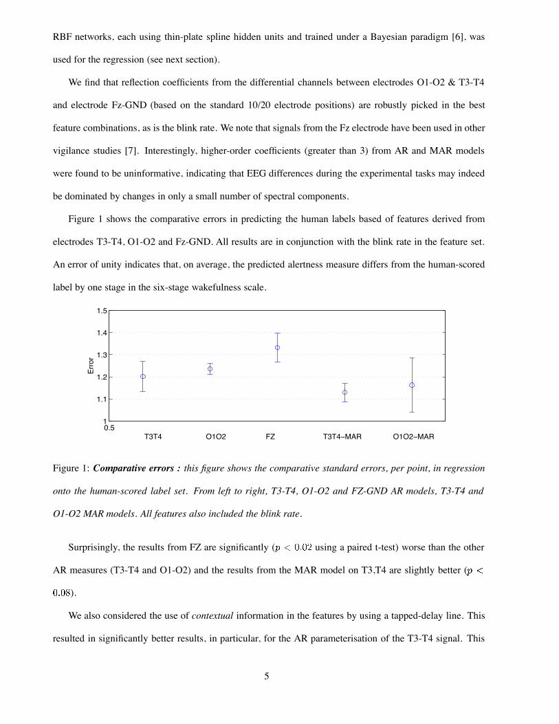
Figure 1 shows the comparative errors in predicting the human labels based of features derived from

electrodes T3-T4, O1-O2 and Fz-GND. All results are in conjunction with the blink rate in the feature set.

An error of unity indicates that, on average, the predicted alertness measure differs from the human-scored

label by one stage in the six-stage wakefulness scale.

0.51

1.1

1.2

1.3

1.4

1.5

Erro

r

T3T4 O1O2 FZ T3T4−MAR O1O2−MAR

Figure 1: Comparative errors : this figure shows the comparative standard errors, per point, in regression

onto the human-scored label set. From left to right, T3-T4, O1-O2 and FZ-GND AR models, T3-T4 and

O1-O2 MAR models. All features also included the blink rate.

Surprisingly, the results from FZ are significantly ( using a paired t-test) worse than the other

AR measures (T3-T4 and O1-O2) and the results from the MAR model on T3,T4 are slightly better (

).

We also considered the use of contextual information in the features by using a tapped-delay line. This

resulted in significantly better results, in particular, for the AR parameterisation of the T3-T4 signal. This

5

improvement was highly significant ( ) and gave rise to mean label errors of . All results

presented in this paper were thence obtained using the first three reflection coefficients from electrodes T3-

T4 and the blink rate measure. A tapped delay line with six taps1, with equally spaced one feature sample

(5s) apart, was used as subsequent input to the analysis system as detailed in the next section. This feature-

extraction formalism is depicted in Figure 2.

X t

ktT3

T4

EOGblink rate

k

bt-T bt

t-T

Figure 2: Feature extraction protocol : the channels T3 and T4 are differenced and AR parameters extracted

from the resultant signal over sucessive 5 second windows ( ). The set of features from a delay line ( )

is formed from these AR parameters along with the blink-rate measure. This combined feature set is thence

utilised as input to the analyser.

2.4 Analysis

Figure 3 shows a typical human-scored labelling, scored into a set of stages on a 15s resolution. Stage 6

is the most ‘awake’ and stage 1 the least. We see that the labelling is characterised by regions of relative

stability and regions of high variability. Regression or classification using this ‘raw’ scoring fails. We

have two choices: firstly we may regard the levels of the human labelling as quantisations of a continuous,1We find that there is little improvement in performance using an increased tap length.

6

smoother, measure and hence represent the time course of the labelling using e.g. a (crude) running mean

and variance measure. We refer to this approach as the regression-based method. The second option is

to take the approach advocated in [8] in which only extremal labels are used to determine the training set.

This assumes that the extremes of e.g. wakefulness and drowsiness are more reliably assessed than the

intermediate states. In this case we take sections of data with labels 5 or 6 to represent alert wakefulness and

sections of data with label 1 to represent a drowsy state. This allows a standard classification approach to

the problem in which alert data may be estimated. We refer to this approach as the extremal-training

method.

0 10 20 30 40 50 601

2

3

4

5

6

t (minutes)

Stag

e

Figure 3: Typical human-scored labelling : Note that the labels are stable for some while at the beginning

of the recording and then become extremely variable.

2.5 Radial Basis Function Analysers

Both regression and classification analysis was performed using committees of Bayesian Radial-Basis Func-

tion (RBF) analysers, as detailed in [6]. The basic theory and methodology may be found in [9] and is only

briefly reviewed here.

We consider the analysis of a datum (feature vector) associated with a target . The RBF operates

by calculating the response of a set of simple non-linear functions to . The functions are often taken to

be Gaussian but in this paper we utilise thin-plate spline functions. The response of the -th such

function is written as

(4)

where in which is the location of the spline function in the feature space. The resultant

7

output of the RBF, conditional on an input and a given set of weights, is thence:

(5)

in which are a set of coupling weights, is a bias weight and a transfer function which is linear

for regression and sigmoidal for classification approaches (see [9] for details). We may write Equation 5 in

terms of a set of latent, or hidden, variables such that

(6)

This is a useful conceptually as we may look easily at the density over as it is linear in the parameters

of the model. Following the approach taken in [6] we utilise a committee of thin-plate spline networks.

Committees of analysers are provably better, on average, than the mean performance of any one analyser

[9] and with randomly located spline positions (i.e. the set of are located at random within the bounds

of the data set) the resultant systems become very rapid to train as the only free parameters of the system

are the weights . When is linear these may be set via a matrix pseudo-inverse approach. When

is sigmoidal, however, a non-linear optimiser must be employed; in all the results presented here we used a

quasi-Newton method based on the BFGS approximations to the Hessian matrix [10].

Equation 5, however, is dependent on the set of weights and in a Bayesian framework these are integrated

out (the Bayesian framework, in essence, aims to remove unknown parameters by integrating over them -

the interested reader is pointed to [11]). Furthermore, a probability density, rather than a point value, may

be obtained. For computational simplicity (and as we have a large training set available) we choose to take

the well-known evidence approach, popularised by MacKay [12, 13] and applied to committees of thin-

plate spline RBFs in [6]. Denoting the output of the analyser to be generated by a mapping from the

latent variable, (Equation 6), the standard evidence framework gives a Gaussian density over with mean

(where is the weight vector of most-probable free parameters i.e. those obtained after

the training process) and variance of:

(7)

in which is the estimated noise variance of the targets (zero in the case of classification),

evaluated at and is the Hessian matrix (the matrix of second derivatives of the error function with

8

respect to the weights - the error functional is least squares for regression and cross-entropy for classification,

see [9] for details) once more evaluated at .

If we take a committee of such analysers, with weighting coefficients , then the probability density on

will be a Gaussian mixture model. We choose to parameterise this model by a moment-matched Gaussian

whose mean is just the weighted average over committee members, i.e.

(8)

and variance given as [6, 14]:

(9)

in which represents the committee variance,

var (10)

the target noise (and residual bias - though this is assumed to be small compared to the target noise for

well-formed models) estimated by:

(11)

and the parameter uncertainty of the committee,

(12)

This is an intuitively pleasing result as the total error may be regarded in a common-sense manner as arising

from three distinct causes.

The first term penalises variant decisions between committee members,

the second penalises the committee as a whole if the output is associated with a region of input space

with high target noise levels

and the third penalises solutions which have poorly set parameters.

In the case of the regression approach, . If we perform a regression, however, onto just the mean

(smoothed) label set we do not take into account the intrinsic variance in the human labelling process (and

9

this is not taken into account in Equation 9). This labelling variance may itself, however, be predicted. We

hence regress onto the two-dimensional target space in which the first target is the mean label value and the

second is the (log) variance in the labelling at that time. We consider the total predictive variance of our

output to be:

(13)

in which the predicted variance of the label set and is given in Equation 9. This approach

may thus be regarded as simple application of mixture density modelling (simple in the sense that a single

component is considered) as detailed in [9], for example.

Although the networks are trained under a Bayesian paradigm, for the classification case we do not allow

high uncertainty (variance) in the latent space to moderate (see [13, 9], for example) the resultant output

probability as this results in the movement of alert for example, to fall towards the class prior of 1/2.

Given that such values are thence interpreted as periods of loss of vigilance we regard this as undesirable.

We note that, as discussed in [6], thin-plate splines have the pragmatic advantage over Gaussians in an

RBF analyser in that their response increases with distance away from the training data set. This means that

the committee variance escalates rapidly in regions outside the training data set hence giving rise to wide

(uncertain) distributions in the latent space. This naturally screens against estimates which are derived from

input data which is inconsistent with that of the training set.

3 Results

In all the results presented below a set of ten RBF networks were used in each committee. The results are

not highly sensitive to the number of committee members and this number was chosen on the grounds of

computational pragmatism. The number of spline functions in each network was set using the evidence

of the model given the training data [12, 9, 6]. For the regression approach this gave rise to networks

with ten splines. For classification eight were sufficient, however. All data are shown smoothed using an

adaptive moving-average filter of length 1 minute (12 feature samples), based on an eigen decomposition of

successive data windows [15]. In the regression case this filtering takes place at the output of the analyser

and in the latent space for classification [16]. For ease of comparison the target label set is also shown

10

smoothed to the same resolution. The training set in all cases consisted of two hours of data from two

subjects who were thence excluded from further analysis.

We present results for both regression and ‘extremal-trained’ classification for three representative sub-

jects. The left-hand plot of each of Figures 4, 5 & 6 shows the regression-based approach with the thick

solid line being the predicted mean and the thin lines at 1 S.D. from this. The thick line of dots (often

hidden behind the prediction) is the (smoothed) human-scored labelling. The right-hand plot of each figure

shows the results of the classification approach, the thick line being the probability of alert wakefulness

(scaled so that a probability of unity maps to label 6 and probability zero to label 1. This enables a direct

comparison with the label set). The label set itself is shown in these plots as the thin solid line. Each plot

consists of four subplots which are the four hour-long recording blocks for each subject.

0 10 20 30 40 50 600

2

4

6

t (minutes)

stat

e

0 10 20 30 40 50 600

2

4

6

t (minutes)

stat

e

0 10 20 30 40 50 600

2

4

6

t (minutes)

stat

e

0 10 20 30 40 50 600

2

4

6

t (minutes)

stat

e

0 10 20 30 40 50 600

2

4

6

t (minutes)

stat

e

0 10 20 30 40 50 600

2

4

6

t (minutes)

stat

e

0 10 20 30 40 50 600

2

4

6

t (minutes)

stat

e

0 10 20 30 40 50 600

2

4

6

t (minutes)

stat

e

Figure 4: Subject A : Analysis based on regression (left-hand four plots) and classification (right-hand four

plots).

We see clearly that both approaches, although not perfect, do track changes in alertness (as defined via

the human-scored labels) reasonably well indicating that alertness may be, in principle, estimated from a

small number of parameters from a single differential EEG channel and eye-movements. We would argue

that although the classification approach gives reasonably good results there are a number of factors which

are not in its favour:

1. As posterior (class) probabilities are being estimated, so point estimates, rather than distributions, are

generated.

11

0 10 20 30 40 50 600

2

4

6

t (minutes)

stat

e

0 10 20 30 40 50 600

2

4

6

t (minutes)

stat

e

0 10 20 30 40 50 600

2

4

6

t (minutes)

stat

e

0 10 20 30 40 50 600

2

4

6

t (minutes)

stat

e0 10 20 30 40 50 60

0

2

4

6

t (minutes)

stat

e

0 10 20 30 40 50 600

2

4

6

t (minutes)

stat

e

0 10 20 30 40 50 600

2

4

6

t (minutes)

stat

e

0 10 20 30 40 50 600

2

4

6

t (minutes)

stat

e

Figure 5: Subject B : Analysis based on regression (left-hand four plots) and classification (right-hand four

plots).

2. As only extreme-labelled data are utilised, the training set is reduced in size.

In the regression approach we see gradual changes in the predicted variance in the vigilance estimate

such as starting around 10 minutes and into the first (uppermost) block of subject A and very large changes

in predicted label variance are observed in subject C (the drowsiest of all the subjects looked at). We also

note the existence of a weak rhythmicity in the vigilance measures (and the smoothed human labels) with

period of order five minutes. This is not an artefact of the filtering or analysis process. The origin of this

oscillation, which we mention is also present in many of the alertness indicators which we have analysed, is

not currently known.

4 Conclusions & future work

The assessment of vigilance from a small number of physiological measurements may be of importance

in safety monitoring in a number of professions. We have shown that ist is possible to make reasonable

estimates of the state of alertness of a subject based on EEG and eye-movement information. The esti-

mates appear to be fairly robust across subjects using appropriately-chosen features from the signals. It is

reiterated, however, that in general neither the smoothed labels (human-scored) nor the resultant estimated

measures correlate well with the corresponding tracking performance measure. Indeed as discussed ear-

lier, the existing experimental data set shows, save for a couple of exceptions, no trends of deterioration in

12

0 10 20 30 40 50 600

2

4

6

t (minutes)

stat

e

0 10 20 30 40 50 600

2

4

6

t (minutes)

stat

e

0 10 20 30 40 50 600

2

4

6

t (minutes)

stat

e

0 10 20 30 40 50 600

2

4

6

t (minutes)

stat

e0 10 20 30 40 50 60

0

2

4

6

t (minutes)

stat

e

0 10 20 30 40 50 600

2

4

6

t (minutes)

stat

e

0 10 20 30 40 50 600

2

4

6

t (minutes)

stat

e

0 10 20 30 40 50 600

2

4

6

t (minutes)

stat

e

Figure 6: Subject C : Analysis based on regression (left-hand four plots) and classification (right-hand four

plots).

tracking performance as the one-hour recording proceeds. What we would ideally like then is to determine

changes in the data which are due to changes in the subjects’ coping strategies as well as true changes in

alertness. We hope that new experimental data will shed light on this.

References

[1] P. Sykacek, I. Rezek, S.J. Roberts, A. Flexer, and G. Dorffner. Bayesian wrappers versus conventional

filters: feature subset selection in the SIESTA project. In Proceedings of EMBEC-99, Vienna, Austria,

November 1999.

[2] M. Pregenzer, S.J. Roberts, and G. Pfurtscheller. Feature selection in the SIESTA project using

DSLVQ. In Proceedings of EMBEC-99, Vienna, Austria, November 1999.

[3] J. Pardey, S. Roberts, and L. Tarassenko. A Review of Parametric Modelling Techniques for EEG

Analysis. Med. Eng. Phys, 18(1):2–11, 1996.

[4] P. Sykacek, I. Rezek, S.J. Roberts, A. Flexer, and G. Dorffner. Reliability in Preprocessing - Bayes

rules. In Proceedings of EMBEC-99, Vienna, Austria, November 1999.

[5] W.J. Krzanowski and F.H.C. Marriott. Multivariate Analysis: Distributions, Ordination and Inference,

volume 1. Edward Arnold, 1994.

13

[6] S.J. Roberts and W. Penny. A Maximum Certainty Approach to Feedforward Neural Networks. Elec-

tronics Letters, 33(4):306–307, 1997.

[7] S. Makeig and M. Inlow. Lapses in alertness: coherence of fluctuations in performance and eeg

spectrum. Electroenceph. Clin. Neur., 86:23–35, 1993.

[8] S. Roberts and L. Tarassenko. New Method of Automated Sleep Quantification. Med. & Biol. Eng. &

Comput., 30(5):509–517, 1992a.

[9] C.M. Bishop. Neural Networks for Pattern Recognition. Oxford University Press, Oxford, 1995.

[10] W.H. Press, B.P. Flannery, S.A. Teukolsky, and W.T. Vetterling. Numerical Recipes in C. Cambridge

University Press, 1991.

[11] J.M. Bernardo and A.F.M. Smith. Bayesian Theory. John Wiley, 1994.

[12] D.J.C. MacKay. A Practical Bayesian Framework for Backpropagation Networks. Neural Computa-

tion, 4:448–472, 1992.

[13] D.J.C. MacKay. The Evidence Framework applied to Classification Networks. Neural Computation,

4:720–736, 1992.

[14] W.D. Penny, D. Husmeier, and S.J. Roberts. The Bayesian Paradigm: second generation neural com-

puting. in: Artificial Neural Networks in Biomedicine, P. Lisboa, I. Ifeachor (Eds.). Springer, 1999.

[15] J. B. Elsner and A. A. Tsonis. Singular Spectrum Analysis: A New Tool in Time Series Analysis.

Plenum Press, New-York, 1996.

[16] S.J. Roberts and W.D. Penny. Real-time Brain Computer Interfacing: a preliminary study using

Bayesian learning. Medical and Biological Engineering & Computing, 38(1):56–61, 2000.

4.0.1 Acknowledgements

The authors would like to thank Will Penny for helpful discussions. Thanks also to Kevin Hapeshi for the

flight simulator software and help with the experimental design. This work was supported by a grant from

BAE SYSTEMS to whom the authors are most grateful.

14