Automated Ball Striker Progress Report for ECSE-4460 Control Systems Design

Team 3 Joseph Black

David Caloccia Gina Rophael Paul Savickas

March 29, 2006 Rensselaer Polytechnic Institute

Executive Summary

This report discusses the progress made in designing and developing a system capable of striking vertically launched ping pong balls toward predetermined targets with precision and accuracy. The system relies on a pan-tilt mechanism with the pan axis utilized for striking ball with a specific velocity, and the tilt axis used to control the angle at which the ball is struck. A launcher has been developed to provide a variable height vertical launch of the ping pong ball. In order to locate the ball and determine when to swing, a webcam will be used with algorithms to find the position of the ball and its velocity. A digital controller will be designed in order to track specific trajectories resulting in the desired position and velocity to strike the ping pong ball. Progress has taken place in various aspects of the development and included: model development, trajectory generation, model validation, friction identification, control development, physical construction, physics model analysis, and subsystem development. In terms of model development, an accurate model of the system was designed to predict its performance and data was compared against actual results in model validation. The system was linearized using state-space equations and was prepared for advanced control design work. LabVIEW motion assistance module was used to verify the trajectory generation. The module will receive a determined strike time from the model for the ball’s launch, and a desired velocity for the paddle from the model of the ball’s flight. From these data points, the paddle must be in the strike zone at a known time with a specified velocity. Experiments were run on both motors to determine the velocity and torque relationship, from which the coefficients of frictions were determined. A complete model of the dynamic system has been developed using PID and LQR controllers for the pan and tilt motors respectively. The mechanical assembly of the paddle to the tilt axis was accomplished, as well as the complete construction of the launcher. A physics model has been determined from the equation for projectile motion of the launch and flight of the ping pong ball, which will be crucial in the calibration of motion between the ball and paddle. The two subsystems of this project are the launcher and vision system. The launcher has been fully constructed after challenges in the assembly, and updates have been made to the vision processing algorithm to determine the location and speed of the ball. There have been a few unanticipated challenges which have led to setbacks in regards to the completion of tasks according to schedule. Most prominently, difficulties in physical construction have led to delays in modeling and control, as well as causing a diversion of effort away from other important tasks which must be accomplished. Comparing the progress made to the projected schedule proposed earlier, the work is up-to-date this week according to the plan. A revised plan was constructed that followed the order in which the tasks were performed and forecasting the tasks yet to be accomplished. Further testing and validation will be taking place and the team is confident that the project objectives will be met, and if time premises higher goals may be manageable. There are three sections in this report which are introduction, preliminary results, and summary of progress and will be discussed respectively in depth.

2

Contents: 1. Introduction………………………………………………………………………….. 6 2. Preliminary Results……………………………………….......................................... 8

2.1 Model Development……………………………………………………….. 8 2.2 Friction Identification.…...….…...………………………………...…......... 9 2.3 Model Validation..….……………………………………………………… 12 2.4 Trajectory Generation..….…….…………………………………………… 12 2.5 Control Development………………………………………………………. 13

2.6 Physical Construction……………………………………………………… 16 2.7 Physics Model……………………………………………………………… 16

2.8 Subsystem Development…………………………………………………… 18 2.8.1 Launcher……….……………………………………………….... 18 2.8.2 Vision System….……………………………………………........ 18

3. Summary of Progress………………………………………....................................... 21 3.1 Comparison with Plan of Action……………………………....................... 21 3.2 Revision of the Schedule…………………………………………............... 21 3.3 Unanticipated challenges……..………………………………..................... 23 3.4 Forecast…………………………………………………………………….. 25

4. Bibliography …………..…………………………………………………………..... 26 5. Statement of Contribution……………………….………………………………….. 27 6. Table of Appendices…..…………………….………………………......................... 28

3

List of Figures: 2.1 Velocity Estimation for the Pan Motor…………………………………………….. 10 2.2 Velocity Estimation for the Tilt Motor…………………………………………….. 10 2.3 Friction Identification for the Pan Motor………………………………………….. 11 2.4 Friction Identification for the Tilt Motor…………………………………….…...... 11 2.5 LabVIEW Motion Assistant Application………………………………………….. 13 2.6 Pan Tilt Nonlinear Simulation……………………………………………………... 14 2.7 Tilt Axis Step Response…………………………………………………………….15 3.1 Preliminary SolidWorks Model for Paddle Assembly……………………………...24 3.2 Current Solid Works Model for Paddle Assembly…………………………............ 24

4

List of Tables: 2.1 Values for Friction for the Pan Motor....…………………………………………… 9 2.2 Values for Friction for the Tilt Motor……………………………………………… 9 3.1 Project Schedule…………………………………………………………………… 22 3.2 Project Task List…………………………………………………………………… 22

5

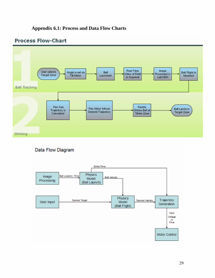
Chapter 1 Introduction: The goal of this project is to create a system capable of striking a vertically launched ping pong ball into the air, and having the ability to control the distance that the ball is hit to. The project can be broken down into three subsystems. The first is the launcher. Goals of this subsystem include the ability to launch a ping pong ball straight up into the air, and to be able to launch the ball to a height of approximately 6 or 7 feet. The second subsystem is the webcam, which will be used to collect data about the ball’s launch, and is part of the ball tracking subsystem. The goal of this subsystem is to analyze frames of the ball’s movement in order to calculate its velocity. The last subsystem uses the pan-tilt mechanism to swing through the strike zone at the same time that the ball is falling through the zone. The major goal of this subsystem is to hit the ball. Other minor goals include controlling the distance that the ball is hit, and being able to provide feedback to the system to adjust its accuracy. Please refer to Appendix 6.1 for process and data flowcharts of the system. Thus far, vast progress has been made towards the full assembling, modeling, testing, and controlling for the Automated Ball Striker system. The mechanical assembly of the paddle to the tilt axis was accomplished, as well as the complete construction of the launcher. A complete model of the dynamic system has been developed using PID and LQR controllers, tests were ran for validation between the simulated and actual model. Progress was also made on the physics model of the system in order to create a calibration between the speed, location of the ball and the appropriate paddle speed needed. The friction of the system has been identified via running the motors at different voltages by which varying the torque input on both axes. Vision testing also took place, and an algorithm was developed to detect the ball, calculate its position and velocity. Comparing the progress made to the projected schedule proposed earlier, the work is up-to-date this week according to the plan. However, the tasks were not completed in the same order as planned which was due to complications in construction of the launcher and testing the tilt axis, which will be discussed in more details in the unanticipated challenges section of this report. Therefore a revised plan was constructed that followed the order in which the tasks were performed and forecasting the tasks yet to be accomplished. The previous week, work was mostly done in assembly, modeling, and validation. This week work will be done mainly in testing. The controllers designed for the pan and tilt will be finally tested on the fully assembled system, aiming for the stability of the system by the end of the week. Calibrations and testing of the vision system with the launcher will also take place this week simultaneously with controller testing.

There have been a few unanticipated challenges which have led to setbacks in regards to the completion of tasks according to schedule. Most prominently, difficulties in physical construction have led to setbacks in modeling and control, as well as causing a diversion of effort away from other important tasks which must be accomplished. Regardless of the setbacks, strong progress is being made toward completion of tasks in order to catch up to the schedule. Due to the many challenges that were not anticipated, the goals of the project are slightly modified with less emphasis on feedback, and more focus on a more adequate controller. Also, higher end goals such as bring a vertically launched ball to rest on the paddle will be eliminated. This goal seems to be a fairly difficult physics and control problem with little relation to the chosen usage of the system; therefore it has a lower priority and is unessential to the success of the system. For the remaining 5 weeks of development, the anticipated goals of each week are very realistic. The revised plan will be followed and if the designed controller works as planned, time will be permissible to work on higher objective regarding feedback, and pitting the machine against a human opponent. Given the current position, these further goals might be possible if work proceeds according to plan.

7

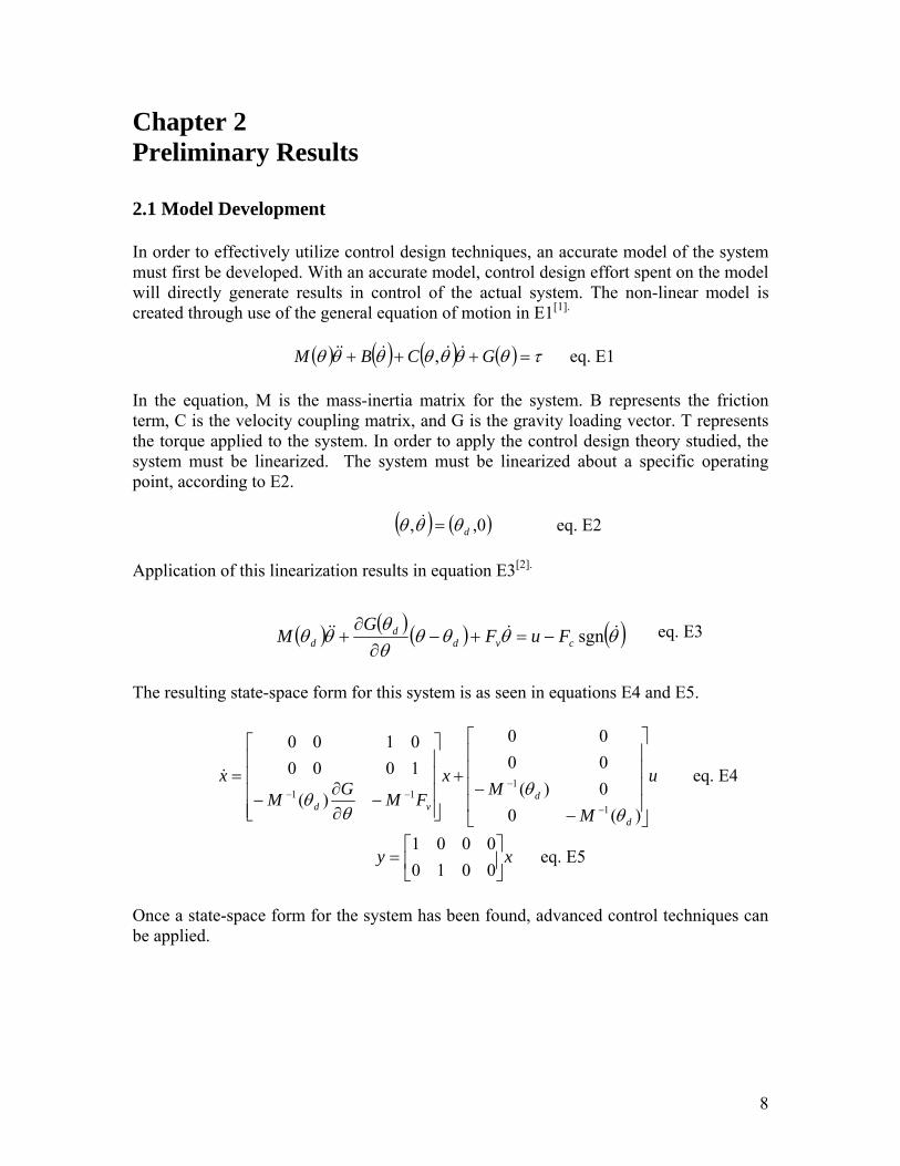
Chapter 2 Preliminary Results 2.1 Model Development In order to effectively utilize control design techniques, an accurate model of the system must first be developed. With an accurate model, control design effort spent on the model will directly generate results in control of the actual system. The non-linear model is created through use of the general equation of motion in E1[1].

( ) ( ) ( ) ( ) τθθθθθθθ =+++ GCBM &&&&& , eq. E1

In the equation, M is the mass-inertia matrix for the system. B represents the friction term, C is the velocity coupling matrix, and G is the gravity loading vector. Τ represents the torque applied to the system. In order to apply the control design theory studied, the system must be linearized. The system must be linearized about a specific operating point, according to E2.

( ) ( )0,, dθθθ =& eq. E2

Application of this linearization results in equation E3[2].

( ) ( ) ( ) ( )θθθθθθ

θθ &&&& sgncvdd

d FuFG

M −=+−∂

∂+ eq. E3

The resulting state-space form for this system is as seen in equations E4 and E5.

u

MM

xFMGM

x

d

dvd ⎥

⎥⎥⎥

⎦

⎤

⎢⎢⎢⎢

⎣

⎡

−−

+

⎥⎥⎥⎥

⎦

⎤

⎢⎢⎢⎢

⎣

⎡

−∂∂

−=

−

−−−

)(00)(0000

)(

1001

0000

1

111

θθ

θθ

& eq. E4

eq. E5 xy ⎥⎦

⎤⎢⎣

⎡=

00100001

Once a state-space form for the system has been found, advanced control techniques can be applied.

8

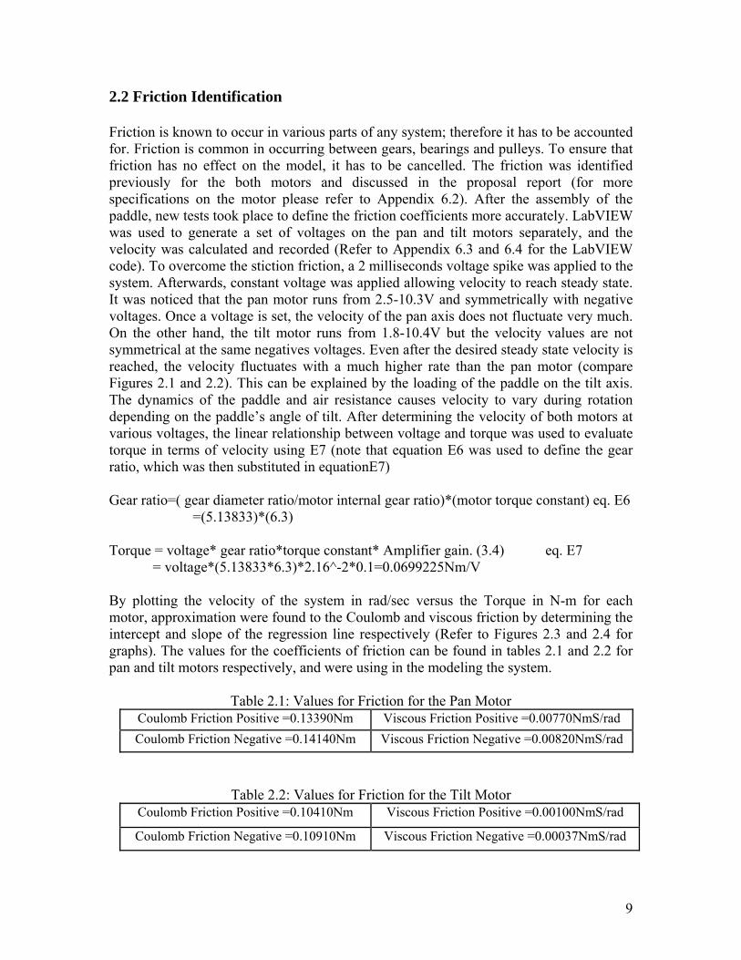
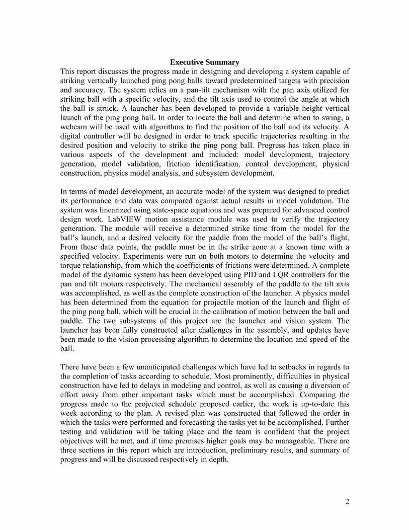
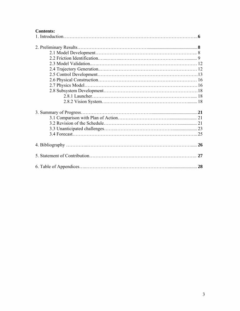
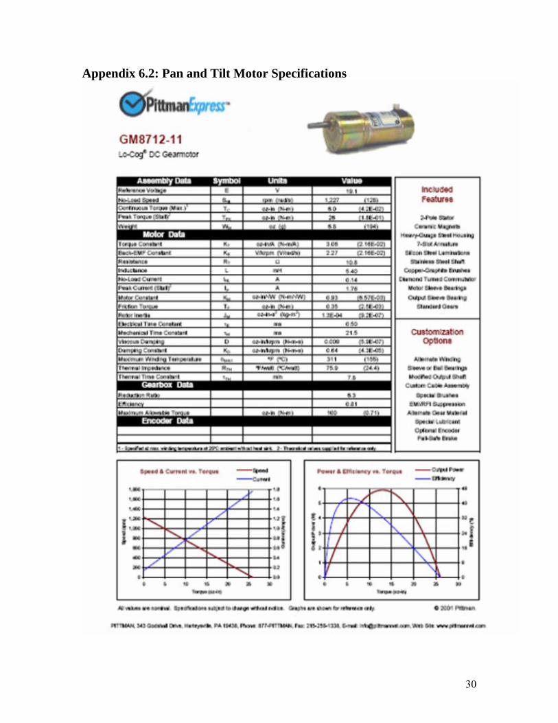
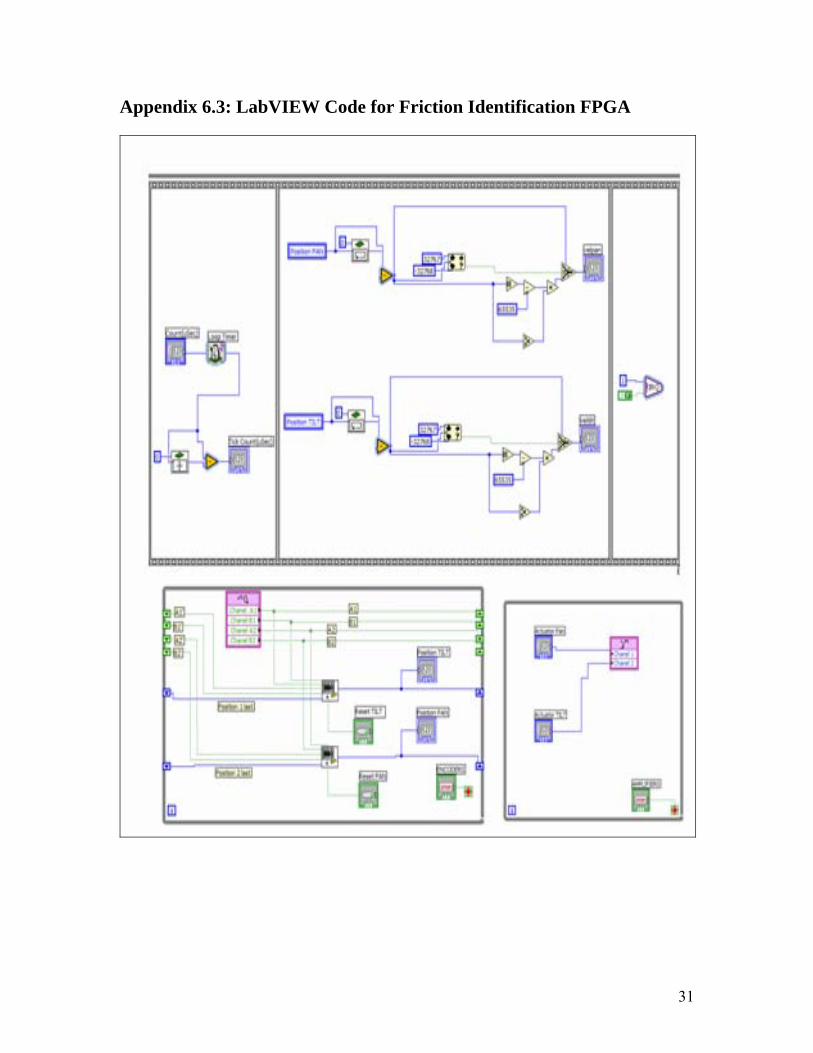
2.2 Friction Identification Friction is known to occur in various parts of any system; therefore it has to be accounted for. Friction is common in occurring between gears, bearings and pulleys. To ensure that friction has no effect on the model, it has to be cancelled. The friction was identified previously for the both motors and discussed in the proposal report (for more specifications on the motor please refer to Appendix 6.2). After the assembly of the paddle, new tests took place to define the friction coefficients more accurately. LabVIEW was used to generate a set of voltages on the pan and tilt motors separately, and the velocity was calculated and recorded (Refer to Appendix 6.3 and 6.4 for the LabVIEW code). To overcome the stiction friction, a 2 milliseconds voltage spike was applied to the system. Afterwards, constant voltage was applied allowing velocity to reach steady state. It was noticed that the pan motor runs from 2.5-10.3V and symmetrically with negative voltages. Once a voltage is set, the velocity of the pan axis does not fluctuate very much. On the other hand, the tilt motor runs from 1.8-10.4V but the velocity values are not symmetrical at the same negatives voltages. Even after the desired steady state velocity is reached, the velocity fluctuates with a much higher rate than the pan motor (compare Figures 2.1 and 2.2). This can be explained by the loading of the paddle on the tilt axis. The dynamics of the paddle and air resistance causes velocity to vary during rotation depending on the paddle’s angle of tilt. After determining the velocity of both motors at various voltages, the linear relationship between voltage and torque was used to evaluate torque in terms of velocity using E7 (note that equation E6 was used to define the gear ratio, which was then substituted in equationE7)

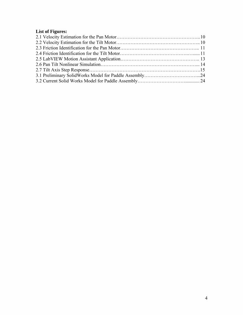
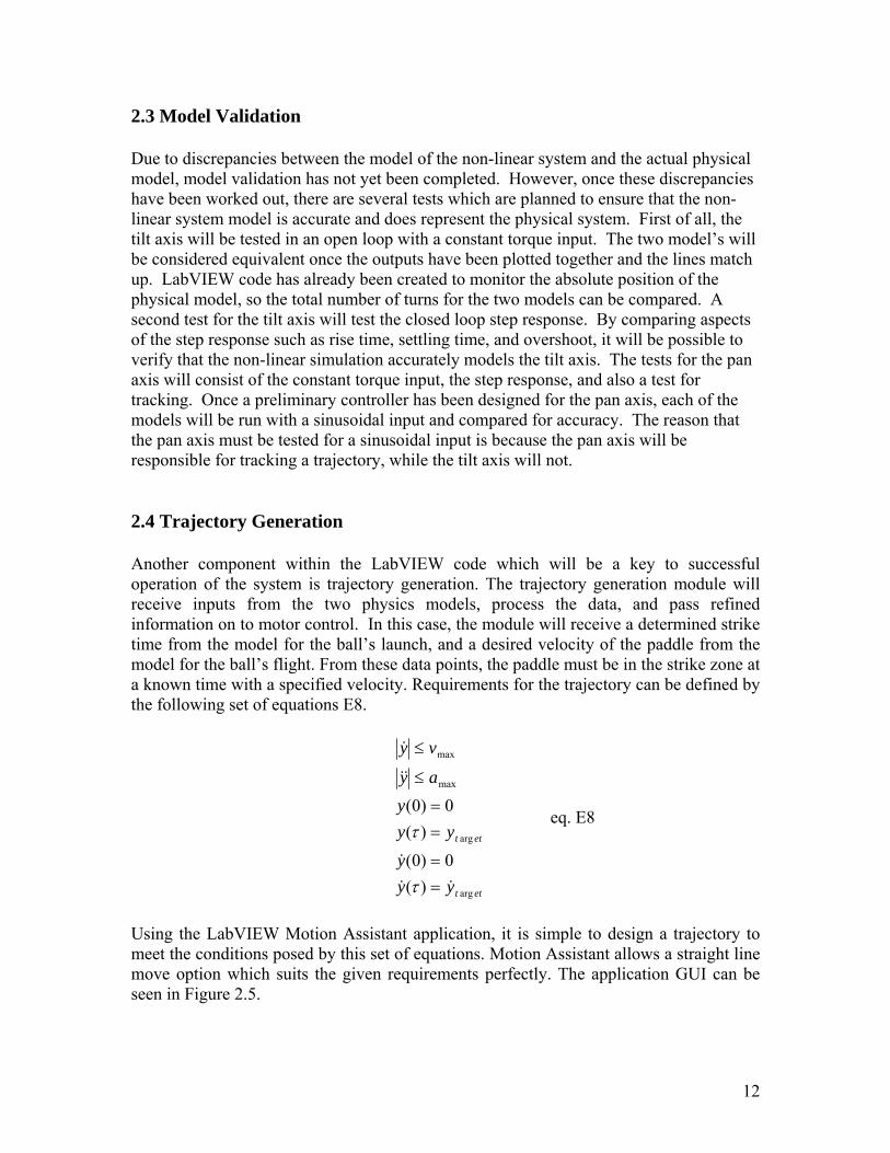
Gear ratio=( gear diameter ratio/motor internal gear ratio)*(motor torque constant) eq. E6 =(5.13833)*(6.3) Torque = voltage* gear ratio*torque constant* Amplifier gain. (3.4) eq. E7 = voltage*(5.13833*6.3)*2.16^-2*0.1=0.0699225Nm/V By plotting the velocity of the system in rad/sec versus the Torque in N-m for each motor, approximation were found to the Coulomb and viscous friction by determining the intercept and slope of the regression line respectively (Refer to Figures 2.3 and 2.4 for graphs). The values for the coefficients of friction can be found in tables 2.1 and 2.2 for pan and tilt motors respectively, and were using in the modeling the system.

Table 2.1: Values for Friction for the Pan Motor

Coulomb Friction Positive =0.13390Nm Viscous Friction Positive =0.00770NmS/rad Coulomb Friction Negative =0.14140Nm Viscous Friction Negative =0.00820NmS/rad

Table 2.2: Values for Friction for the Tilt Motor Coulomb Friction Positive =0.10410Nm Viscous Friction Positive =0.00100NmS/rad

Coulomb Friction Negative =0.10910Nm Viscous Friction Negative =0.00037NmS/rad

9

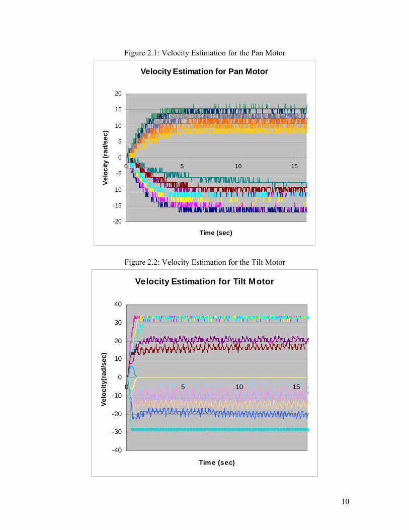
Figure 2.1: Velocity Estimation for the Pan Motor

Velocity Estimation for Pan Motor

-20

-15

-10

-5

0

5

10

15

20

0 5 10 1

Time (sec)

Velo

city

(rad

/sec

)

5

Figure 2.2: Velocity Estimation for the Tilt Motor

Velocity Estimation for Tilt Motor

-40

-30

-20

-10

0

10

20

30

40

0 5 10 15

Time (sec)

Velo

city

(rad

/sec

)

10

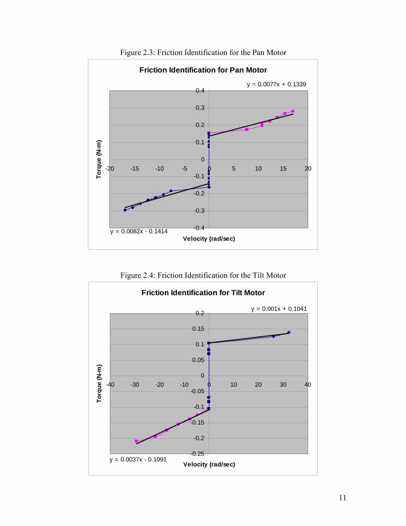
Figure 2.3: Friction Identification for the Pan Motor

Friction Identification for Pan Motor

y = 0.0077x + 0.1339

y = 0.0082x - 0.1414 -0.4

-0.3

-0.2

-0.1

0

0.1

0.2

0.3

0.4

-20 -15 -10 -5 0 5 10 15 20

Velocity (rad/sec)

Torq

ue (N

-m)

Figure 2.4: Friction Identification for the Tilt Motor

Friction Identification for Tilt Motor

y = 0.001x + 0.1041

y = 0.0037x - 0.1091-0.25

-0.2

-0.15

-0.1

-0.05

0

0.05

0.1

0.15

0.2

-40 -30 -20 -10 0 10 20 30 40

Velocity (rad/sec)

Torq

ue (N

-m)

11

2.3 Model Validation Due to discrepancies between the model of the non-linear system and the actual physical model, model validation has not yet been completed. However, once these discrepancies have been worked out, there are several tests which are planned to ensure that the non-linear system model is accurate and does represent the physical system. First of all, the tilt axis will be tested in an open loop with a constant torque input. The two model’s will be considered equivalent once the outputs have been plotted together and the lines match up. LabVIEW code has already been created to monitor the absolute position of the physical model, so the total number of turns for the two models can be compared. A second test for the tilt axis will test the closed loop step response. By comparing aspects of the step response such as rise time, settling time, and overshoot, it will be possible to verify that the non-linear simulation accurately models the tilt axis. The tests for the pan axis will consist of the constant torque input, the step response, and also a test for tracking. Once a preliminary controller has been designed for the pan axis, each of the models will be run with a sinusoidal input and compared for accuracy. The reason that the pan axis must be tested for a sinusoidal input is because the pan axis will be responsible for tracking a trajectory, while the tilt axis will not. 2.4 Trajectory Generation Another component within the LabVIEW code which will be a key to successful operation of the system is trajectory generation. The trajectory generation module will receive inputs from the two physics models, process the data, and pass refined information on to motor control. In this case, the module will receive a determined strike time from the model for the ball’s launch, and a desired velocity of the paddle from the model for the ball’s flight. From these data points, the paddle must be in the strike zone at a known time with a specified velocity. Requirements for the trajectory can be defined by the following set of equations E8.

ett

ett

yyy

yyy

ay

vy

arg

arg

max

max

)(0)0(

)(0)0(

&&

&

&&

&

==

==

≤

≤

τ

τ eq. E8

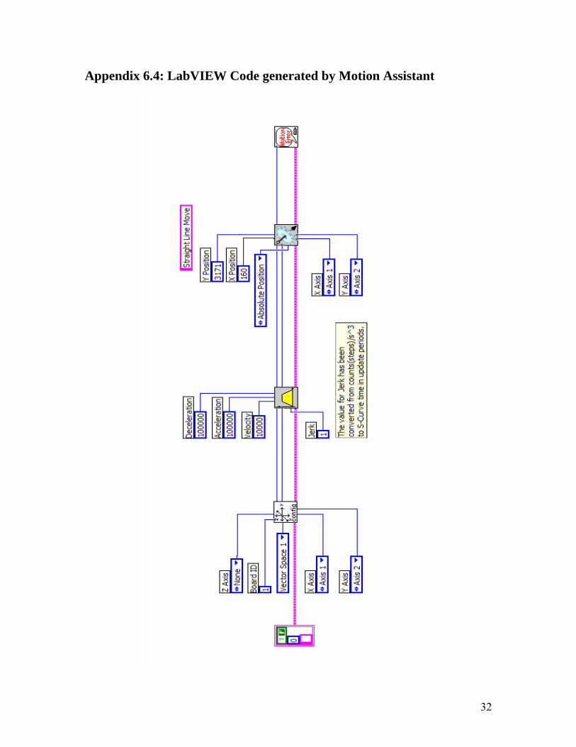
Using the LabVIEW Motion Assistant application, it is simple to design a trajectory to meet the conditions posed by this set of equations. Motion Assistant allows a straight line move option which suits the given requirements perfectly. The application GUI can be seen in Figure 2.5.

12

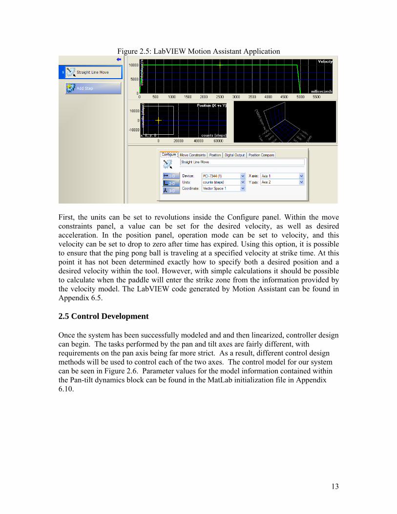
Figure 2.5: LabVIEW Motion Assistant Application

First, the units can be set to revolutions inside the Configure panel. Within the move constraints panel, a value can be set for the desired velocity, as well as desired acceleration. In the position panel, operation mode can be set to velocity, and this velocity can be set to drop to zero after time has expired. Using this option, it is possible to ensure that the ping pong ball is traveling at a specified velocity at strike time. At this point it has not been determined exactly how to specify both a desired position and a desired velocity within the tool. However, with simple calculations it should be possible to calculate when the paddle will enter the strike zone from the information provided by the velocity model. The LabVIEW code generated by Motion Assistant can be found in Appendix 6.5. 2.5 Control Development Once the system has been successfully modeled and and then linearized, controller design can begin. The tasks performed by the pan and tilt axes are fairly different, with requirements on the pan axis being far more strict. As a result, different control design methods will be used to control each of the two axes. The control model for our system can be seen in Figure 2.6. Parameter values for the model information contained within the Pan-tilt dynamics block can be found in the MatLab initialization file in Appendix 6.10.

13

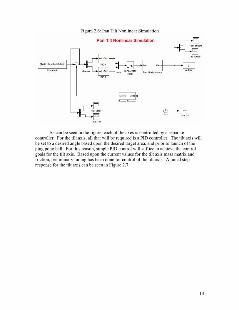
Figure 2.6: Pan Tilt Nonlinear Simulation

As can be seen in the figure, each of the axes is controlled by a separate controller. For the tilt axis, all that will be required is a PID controller. The tilt axis will be set to a desired angle based upon the desired target area, and prior to launch of the ping pong ball. For this reason, simple PID control will suffice to achieve the control goals for the tilt axis. Based upon the current values for the tilt axis mass matrix and friction, preliminary tuning has been done for control of the tilt axis. A tuned step response for the tilt axis can be seen in Figure 2.7.

14

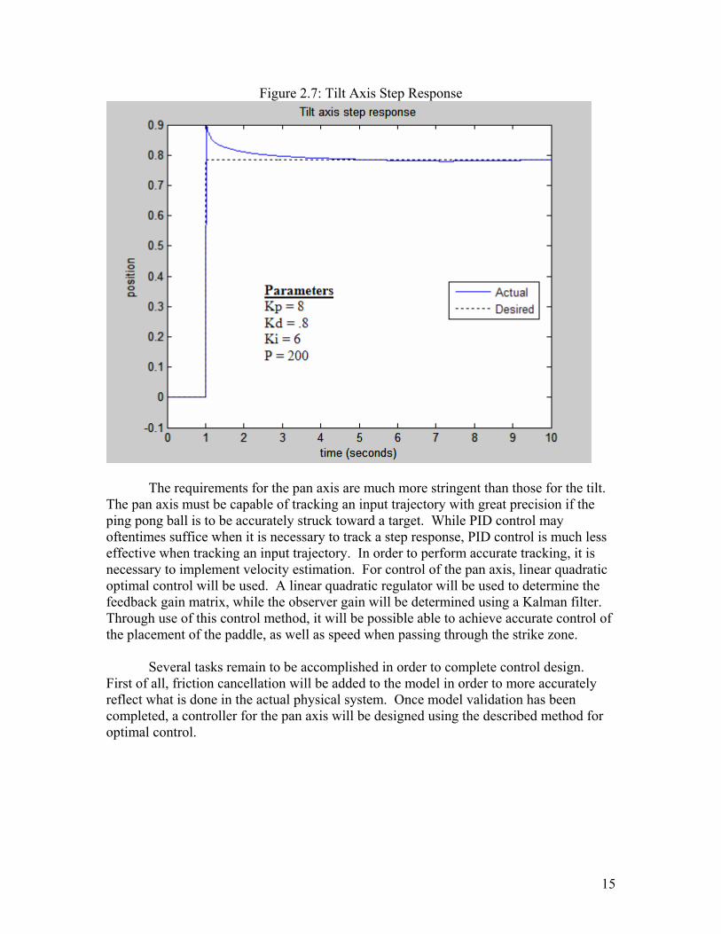
Figure 2.7: Tilt Axis Step Response

The requirements for the pan axis are much more stringent than those for the tilt. The pan axis must be capable of tracking an input trajectory with great precision if the ping pong ball is to be accurately struck toward a target. While PID control may oftentimes suffice when it is necessary to track a step response, PID control is much less effective when tracking an input trajectory. In order to perform accurate tracking, it is necessary to implement velocity estimation. For control of the pan axis, linear quadratic optimal control will be used. A linear quadratic regulator will be used to determine the feedback gain matrix, while the observer gain will be determined using a Kalman filter. Through use of this control method, it will be possible able to achieve accurate control of the placement of the paddle, as well as speed when passing through the strike zone. Several tasks remain to be accomplished in order to complete control design. First of all, friction cancellation will be added to the model in order to more accurately reflect what is done in the actual physical system. Once model validation has been completed, a controller for the pan axis will be designed using the described method for optimal control.

15

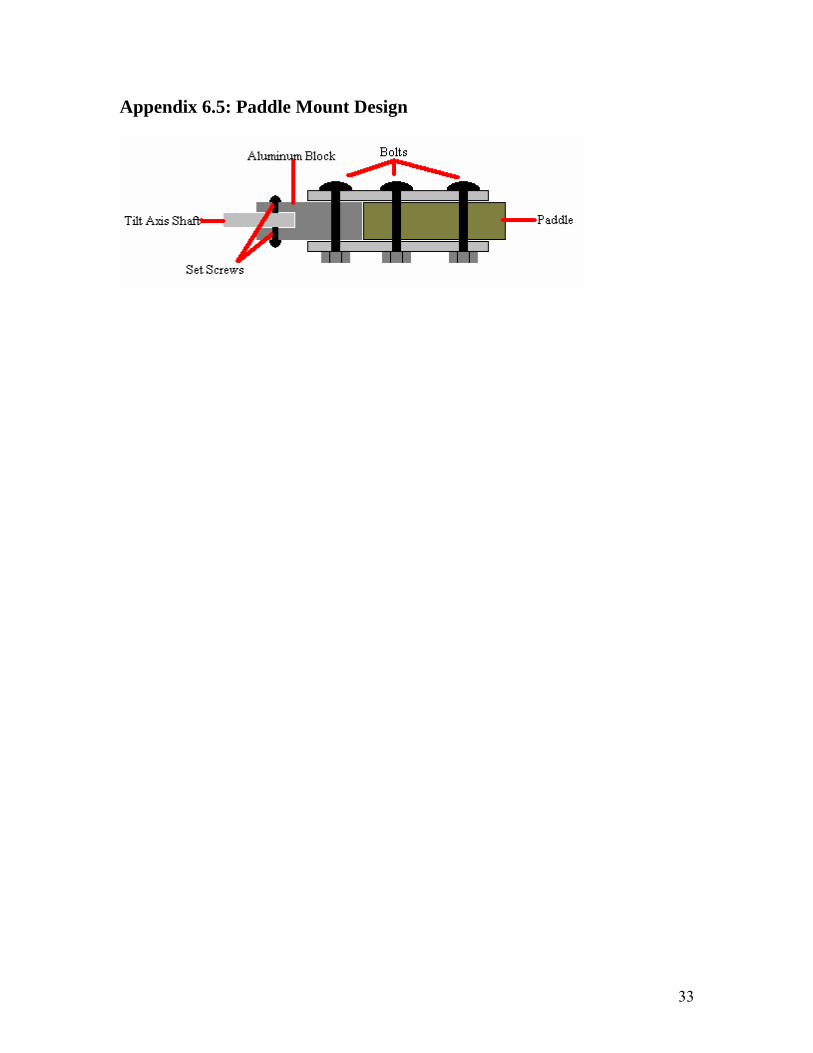
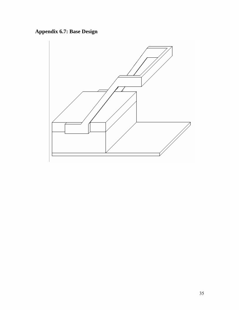
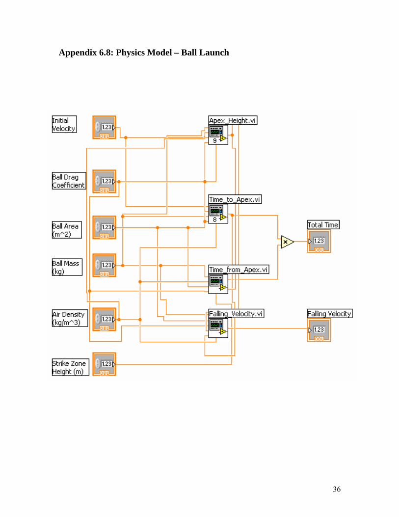
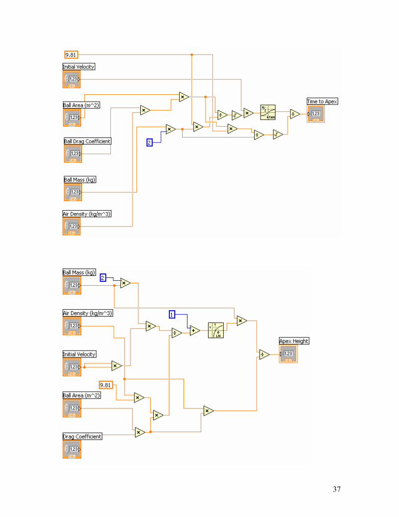
2.6 Physical Construction The three major parts that needed construction were the paddle mount, the launcher, and the base. As soon as the idea of the project was developed, work on design and assembly took place. The design was changed several times however, to ensure the best stability of the system. Currently, the paddle mount and launcher have both been completed, and the base is yet to be built. The original design of the paddle mount included two clamps which were to be used to fix the paddle to the tilt axis shaft. However, the clamps needed to be altered in order to be used, and were damaged during the machining. This caused changes to the preliminary design. To replace the clamps, an aluminum block was machined to hold the paddle to the tilt axis shaft. A drawing of the new design can be seen in Appendix 6.8. Please refer to Appendix 6.9 for dimensions. The design of the launcher has also changed as the project has progressed. The initial design had the ball resting on the platform, but this design did not launch the ball to a sufficient height. In order to get the ball high enough, the design was changed so that the ball is now suspended in the tube and is struck by the platform. This new design can be seen in Appendix 6.7. The design and construction of the base has not yet been fully completed. Most of the system’s functionality can be tested without the base, so its construction has been suspended while other parts have been worked on. A preliminary design of the base can be seen in Appendix 6.9. 2.7 Physics Model Modeling the launch and flight of the ping pong ball is crucial for the system’s performance. These models will determine at what time the paddle and ball will need to meet, and how far the ball will travel once it is struck. The models will be created from equations for projectile motion. These equations must compensate for air resistance, since it greatly affects a ping pong ball. Since air resistance is proportional to the square of the velocity, a differential equation must be solved in order to determine the speed and position of the ball. Also, air resistance opposes the direction of motion, which results in two different equations. One equation is for the ball as it rises (eq. E9), and the other is for the ball as it falls (eq. E10)

[3].

16

( ⎟⎟⎠

⎞⎜⎜⎝

⎛−⎟⎟

⎠

⎞⎜⎜⎝

⎛⎟⎟⎠

⎞⎜⎜⎝

⎛= tt

mCAg

CAmgtv a2

tan2)( ρρ

) eq. E9

( )⎟⎟⎠

⎞⎜⎜⎝

⎛−⎟⎟

⎠

⎞⎜⎜⎝

⎛⎟⎟⎠

⎞⎜⎜⎝

⎛= tt

mCAg

CAmgtv a2

tanh2)( ρρ

eq. E10

m = mass of ball g = force of gravity ρ = density of air C = drag coefficient of ball[4]

A = cross-sectional area of ball ta = time from ground to apex of launch (eq. E11)

mCAg

mgCAv

to

a

2

2arctan

ρ

ρ⎟⎟⎠

⎞⎜⎜⎝

⎛

= eq. E11

vo = initial velocity of ball

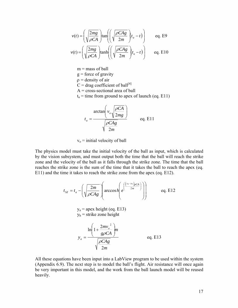
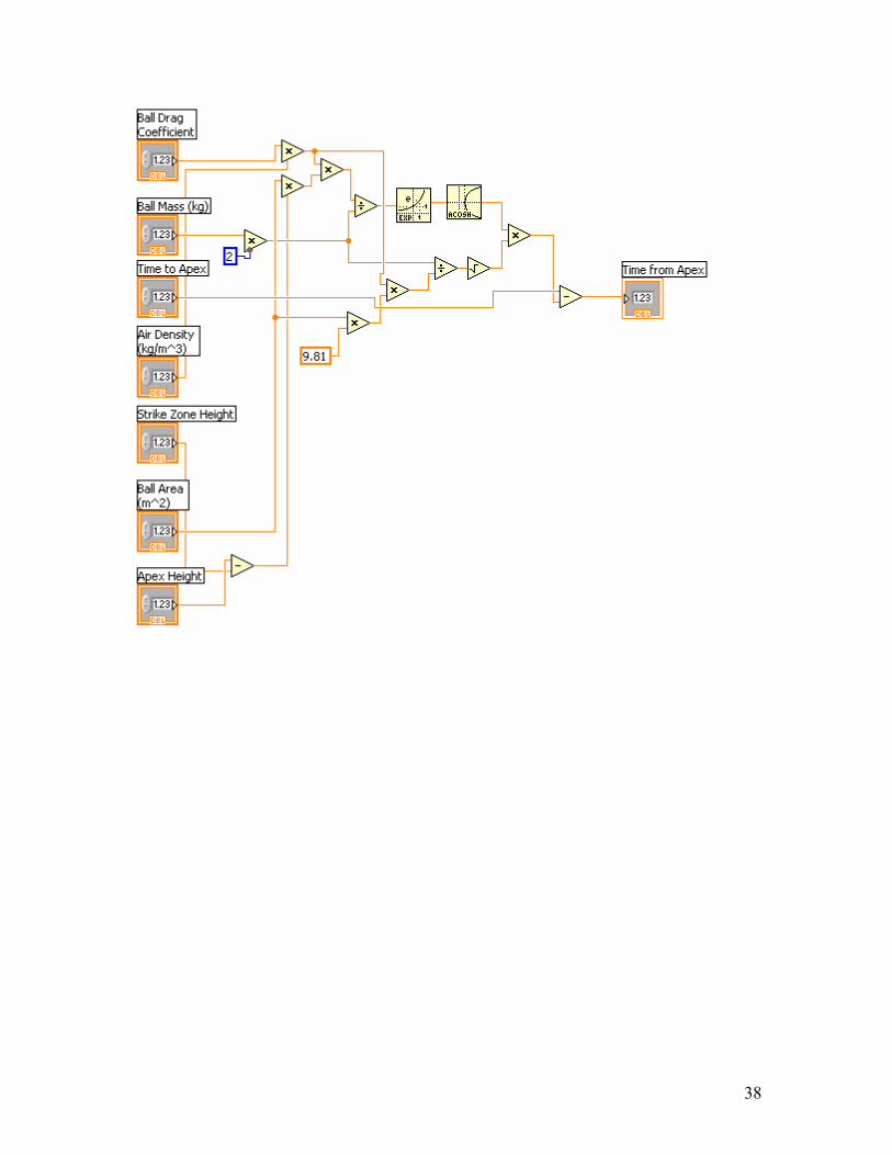
The physics model must take the initial velocity of the ball as input, which is calculated by the vision subsystem, and must output both the time that the ball will reach the strike zone and the velocity of the ball as it falls through the strike zone. The time that the ball reaches the strike zone is the sum of the time that it takes the ball to reach the apex (eq. E11) and the time it takes to reach the strike zone from the apex (eq. E12).

( )

⎟⎟⎟

⎠

⎞

⎜⎜⎜

⎝

⎛

⎟⎟⎟

⎠

⎞

⎜⎜⎜

⎝

⎛

⎟⎟⎠

⎞⎜⎜⎝

⎛−=

⎟⎟⎠

⎞⎜⎜⎝

⎛ −

mCA

aSZ

hyay

ehCAg

mtt 2arccos2ρ

ρ eq. E12

ya = apex height (eq. E13) yh = strike zone height

mCAg

mCAg

mv

y

o

a

2

21ln

2

ρ

ρ ⎟⎟⎠

⎞⎜⎜⎝

⎛+

= eq. E13

All these equations have been input into a LabView program to be used within the system (Appendix 6.9). The next step is to model the ball’s flight. Air resistance will once again be very important in this model, and the work from the ball launch model will be reused heavily.

17

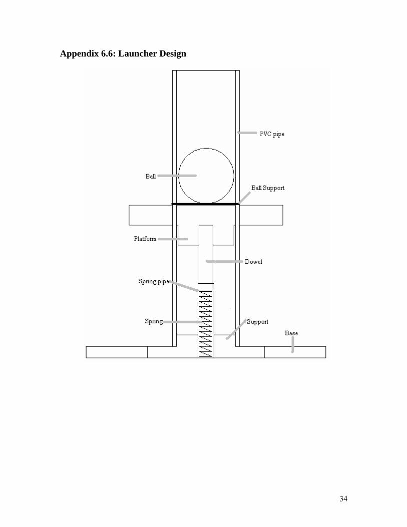
2.8 Subsystem 2.8.1 Launcher In order to hit the ball with the paddle, the ball must first be launched into the air. To do this, a spring loaded launcher has been designed and constructed. The launcher was built using a PVC pipe as the barrel, a steel pipe to house the spring, a wooden dowel to compress the spring, and a waterjet cut piece of Lexan as a platform to strike the ball. The original idea was to have the ball rest on the platform, but after a few tests, it was found that the ball would need to be initially at rest and then struck by the platform in order to be launched to a sufficient height. A diagram showing the individual pieces of the launcher can be found in Appendix 6.7. Substantial progress has been made on the design and construction of the ping pong ball launcher. After a few minor setbacks, the launcher has been fully constructed and is ready to be attached to the base. Only a small amount of testing has been done with the launcher, but it has been determined that the launcher is capable of launching the ball to a sufficient height. There has been some trouble with getting the ball to launch vertically in a straight line, but this should be corrected when it is attached to the base. 2.8.2 Vision System Improvements have been made in the vision system, with yet more to be accomplished. The initial LabVIEW code for image processing and velocity calculation of the ball was constructed. The system will have a pre-calibrated image of the area of interest with the information to convert Pixels to real world measurements. So far the calibration method has been using LabVIEW’s simple calibration, where a ruler with two points of known distance was used and feed information back to the program with the distance between the two points. Testing of the distance measurement among other points of the ruler had the accuracy of a 10th of an inch. This calibration was then saved and reused for the remainder of the image processing work needed. In order to determine the ball speed and velocity, a LabVIEW code was designed to do so and this will be discussed in this section. When an image is first acquired, the image and a tick count of milliseconds are recorded into a clustered bundle of data in LabVIEW. This bundle should have a record of the image and the millisecond tick counter saved simultaneously. Afterwards the webcam will continue to take pictures and the most recent image will be processed with the calibration information imported, and the image will be masked, leaving only desired regions of interests, which is the path of the ball’s flight. For the detection of the ball, there will be a black background which the ball will be launched against.

18

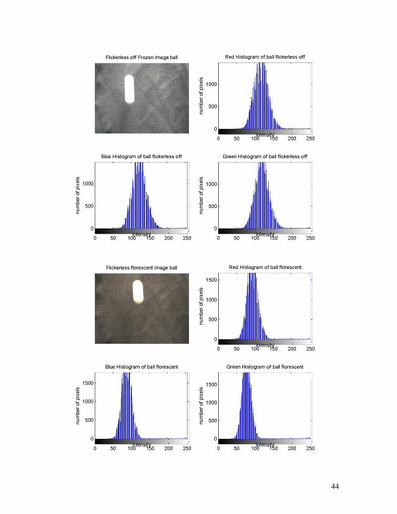
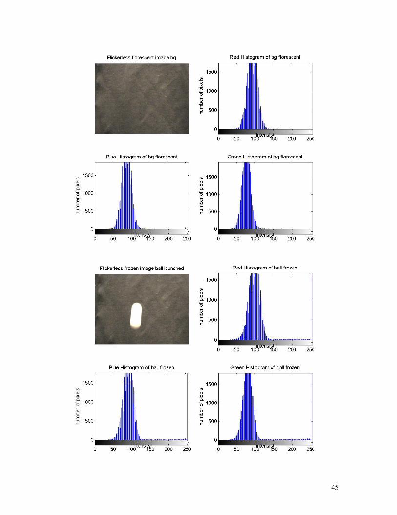
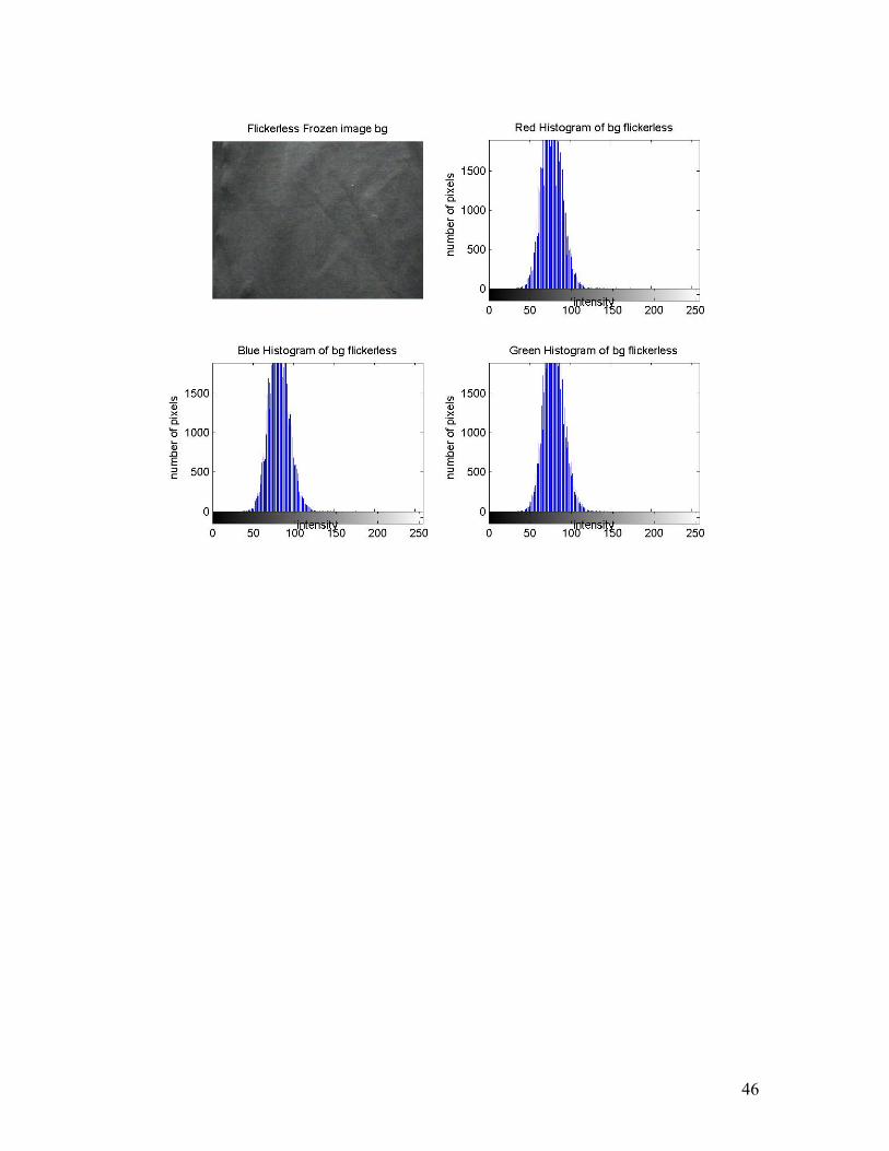
The Labview USB Vision uses the webcam drivers on the windows machine to acquire the images and some of the initial processing. The Logitech drivers for our particular webcam had some additional settings that can be changed, unfortunately the exposure settings are unchangeable but there is settings for lighting and a flickerless mode. After some testing with various modes, it has been found that flickerless mode makes the black background blacker and doesn’t affect the color of the white ball see figures of flickelessr on and flickerless off. The flickerless mode is design to remove the 60 hz flicker of a florescent light. It needs further testing but seems the flickerless mode decreases the blurriness of images, but more testing is required of this phenomena. There is also various lighting effects of Frozen, Florescent, daylight, and incandescent. Had Tested Frozen and Florescent with histogram shown in figures, daylight and incandescent lightens the black bg pretty clearly. The histograms of Florscent vs Frozen with flickerless on shows that the frozen pushes the black background further towards the lower intensity and smoothes out. This allows us to run with threshold of 150 minimal and with the ball images it clearly seen most of the pixels of the ball are in 255 range. The ball is very distinct from the background. A 150 to 255 Threshold for all three colors is clearly doable for processing the image. (See Appendix 6.11) Histograms of the background have shown that almost all the background has a color threshold below 141 in red and green, but dirt and other particles on the background brings up the blue threshold to 210 (See Appendix 6.11). The ping pong ball launched will be either of the color white or green, and both have histograms with most of the pixels above these threes hold values, therefore it will be quite distinct from the background. The initial threshold of the image creates a binary image of the ball and may have a few other particles of dirt on the background highlighted, but these extraneous objects can easily be removed by filtering the binary image area for the size and orientation of the particles. The orientation is the direction of the object, where the direction of the ball from the launching and the blur will have a vertical orientation. After this filtration there should only be one object left in the image, which will be the ball if in sight. The code will use LabVIEW Particle analysis to return the position of the particle in real world measurements recording the top of the particle. If there is 1 particle in the image the LabVIEW code will go into the velocity calculation part of the vision code. The code will check if the previous iteration has detected a particle if not it goes only into the first condition of the velocity determination where the data will be recorded for use in the next iteration. The next iteration if the ball was detect in the current and the past will have the velocity go into the next section of the velocity determination, where the code takes the new time stamp values and position values and subtract the old values from them. Then divide the position difference by the timestamp difference to determine velocity, which will be fed into the physics model. But current code records the position, velocity and time difference into a data file for review.

19

A current challenge with the code written up-to-date is the inability of saving the images of when the ball in sight for further review. Although saving of the images can cause delays in the code as it attempts to compose the image file, but saving the image would be useful for testing purposes and ensuring that the code is working properly. The current code will still need extensive testing of the timestamps, velocity calculations and image capture of the ball launched with the launcher, as opposed to tossed and dropped into field of view. The time costs of the processing and image acquisition will also need to be calculated, the processing has been calculated thru LabVIEW Vision Assistant to be approximately 300 units per second, which is faster than acquiring the image at 30 frames a second. Next, an advanced calibration method of using a dot matrix with a known spacing between dots will be used, which should provide higher accuracy. This will be done by acquiring an image of the calibration sheet provided by LabVIEW in the plane of the launch and specify the threshold and spacing of dots. LabVIEW will then form a superior calibration taking into account possible distortion caused by the lens and other factors. All this information will then be saved into an image that will loaded by LabVIEW code for calibration information that can be imported later when calibration is necessary. The possibility of using the length of the streak to determine instantaneous velocity is being considered. The drivers of the Logitech pro 4000 webcam that is being used have the option of changing the exposure rate to a time frame but changing it does not seem to have a lasting effect. After the window is closed, the exposure rate goes back to the automatic setting, which takes into account the lighting conditions. The calculation of the length of exposure will need to be tested and determined, methods of testing this could be potentially using a pendulum with a known weight and drop height, with a speed that can be calculated to determine exposure rate. Another possibility is using an electric screw driver or the tilt axis, with a string tied around the axis to pull up and lower the ball with a calculable speed in front of the webcam. Both methods can be used to determine the exposure length for instantaneous speed calculations and also velocity determination from multiple frame grabbing.

20

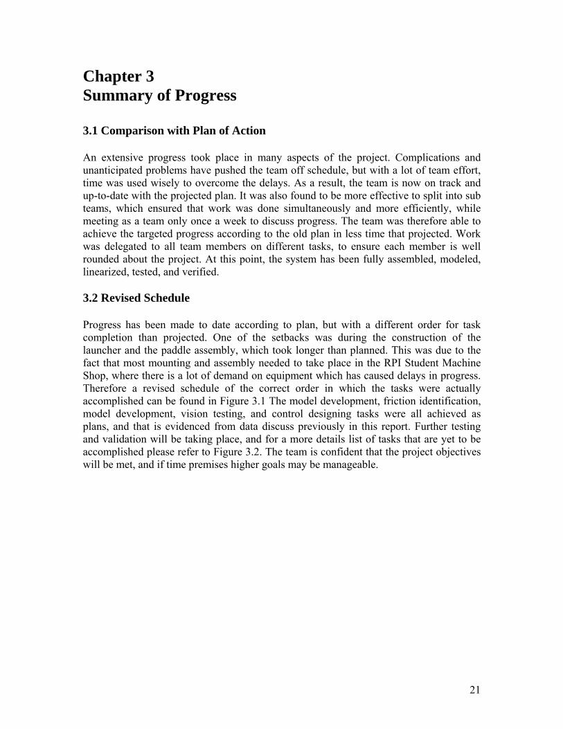
Chapter 3 Summary of Progress 3.1 Comparison with Plan of Action An extensive progress took place in many aspects of the project. Complications and unanticipated problems have pushed the team off schedule, but with a lot of team effort, time was used wisely to overcome the delays. As a result, the team is now on track and up-to-date with the projected plan. It was also found to be more effective to split into sub teams, which ensured that work was done simultaneously and more efficiently, while meeting as a team only once a week to discuss progress. The team was therefore able to achieve the targeted progress according to the old plan in less time that projected. Work was delegated to all team members on different tasks, to ensure each member is well rounded about the project. At this point, the system has been fully assembled, modeled, linearized, tested, and verified. 3.2 Revised Schedule Progress has been made to date according to plan, but with a different order for task completion than projected. One of the setbacks was during the construction of the launcher and the paddle assembly, which took longer than planned. This was due to the fact that most mounting and assembly needed to take place in the RPI Student Machine Shop, where there is a lot of demand on equipment which has caused delays in progress. Therefore a revised schedule of the correct order in which the tasks were actually accomplished can be found in Figure 3.1 The model development, friction identification, model development, vision testing, and control designing tasks were all achieved as plans, and that is evidenced from data discuss previously in this report. Further testing and validation will be taking place, and for a more details list of tasks that are yet to be accomplished please refer to Figure 3.2. The team is confident that the project objectives will be met, and if time premises higher goals may be manageable.

21

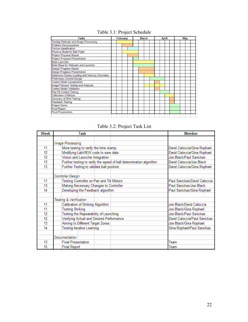
Table 3.1: Project Schedule

Table 3.2: Project Task List

22

3.3 Unanticipated Challenges In the development of the system, several unforeseen challenges have presented themselves and posed as a hindrance to forward progress. Foremost, the physical construction of the system has proved to be a far more difficult task than was originally expected. With very little mechanical or machining experience on the team, along with no experience in materials, it has been quite difficult to design and build effective mechanical components. An example of problems encountered lies within the development of a ping pong ball launcher. The launcher was originally designed with materials which were not strong enough to withstand the impact of launching, and which had to be replaced. Another difficulty arises from the fact that while a great deal of time was spent in carefully designing the launcher to provide a consistent vertical launch, the launcher has yet to perform according to the specifications. A second mechanical problem arose during the machining of a mounting apparatus for the ping pong paddle. The design for mounting the paddle called for two small rings which fit on to the tilt axis to be machined flat and then drilled through and threaded in order to mount a bracket. The bracket was to connect the rings to the ping pong paddle, thereby fixing it to the tilt axis (refer to assembly in Figure 3.1). However, the holes in the rings were drilled slightly off center, eventually rendering the rings useless and requiring improvisation of a completely new mounting mechanism for the paddle (Figure 3.2). Another challenge lies within the overall layout of the system. The success of the system relies on the three subsystems, and their successful interaction with each other. Key to that interaction is careful consideration of the spacing necessary between components to allow the webcam ample time to view the launch, and to maintain a vertical launch within range of the paddle. A great deal of time and effort has already been spent toward construction of the base, and more time continues to be spent. There have been problems with the FPGA reading from the encoders at high sampling speeds and slow rotation speeds. At a speed of one rotation per second there are 4096 tick marks per second. At a sampling speed of 1 ms , the encoder will count only 4096*.001=4 ticks per ms. At greater sampling speeds the FPGA counts fewer ticks until the point where it counts only 0 or 1, resulting from the sampling being faster than the rotation of ticks. To counter this issue the FPGA sampling rate was slowed down to 1 ms. An alternative solutions is averaging the FPGA data to calculate velocity. The nature of the FPGA makes averaging calculations tough, because it can not perform floating point division. Instead, the data must be stored and transferred to the host for averaging. The storage can be done by using a FIFO system on the FPGA. However issues with memory space usage can often arise when using this approach. The sampling rate of 1 ms is best for the system and allows the FPGA to record the encoders and calculate the difference without need of data storage. Also, the FPGA loop is able to run in consistent time, because no operation in the FPGA should slow it down beyond the 1 ms loop cycle.

23

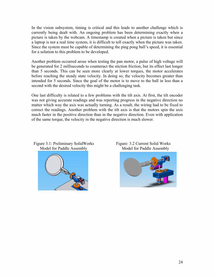
In the vision subsystem, timing is critical and this leads to another challenge which is currently being dealt with. An ongoing problem has been determining exactly when a picture is taken by the webcam. A timestamp is created when a picture is taken but since a laptop is not a real time system, it is difficult to tell exactly when the picture was taken. Since the system must be capable of determining the ping pong ball’s speed, it is essential for a solution to this problem to be developed. Another problem occurred arose when testing the pan motor, a pulse of high voltage will be generated for 2 milliseconds to counteract the stiction friction, but its effect last longer than 5 seconds. This can be seen more clearly at lower torques, the motor accelerates before reaching the steady state velocity. In doing so, the velocity becomes greater than intended for 5 seconds. Since the goal of the motor is to move to the ball in less than a second with the desired velocity this might be a challenging task. One last difficulty is related to a few problems with the tilt axis. At first, the tilt encoder was not giving accurate readings and was reporting progress in the negative direction no matter which way the axis was actually turning. As a result, the wiring had to be fixed to correct the readings. Another problem with the tilt axis is that the motors spin the axis much faster in the positive direction than in the negative direction. Even with application of the same torque, the velocity in the negative direction is much slower. Figure 3.1: Preliminary SolidWorks Figure: 3.2 Current Solid Works Model for Paddle Assembly Model for Paddle Assembly

24

3.4 Forecast Given the current position in progress and with a reasonable forecast for the remainder of the development process, the minimal targeted goal of ball striking will be achieved. The team is willing to spend time and effort to ensure that the current challenges and problems are resolved, but currently it’s unknown whether or not the system will be able to overcome the identified problems.

25

Chapter 4 Bibliography

1. Wen, John T. “ECSE 4460 Control System Design, Spring 2006”. Internet. (2006)

Available: http://www.cats.rpi.edu/%7Ewenj/ECSE446S06/modeling.pdf 2. Wen, John T. “ECSE 4460 Control System Design, Spring 2006”. Internet. (2006)

Available: http://www.cats.rpi.edu/%7Ewenj/ECSE4962S04/final/team2finalreport.pdf

3 Israel, Robert. “Pop Flies: The Sequel,” Internet (1997) Available: http://www.math.ubc.ca/~israel/m215/baseball/baseball.html

4. Weisstein, Eric. “Drag Coefficients” Internet (2006) Available:

http://scienceworld.wolfram.com/physics/DragCoefficient.html

26

Chapter 5 Statement of Contribution For this Project Proposal Report: Joseph Black has completed the following sections:

• Introduction • Physics Model • Physical Construction • Subsystem Development: Launcher • Report Editing

David Caloccia has completed the following sections: • Subsystem Development: Vision • Model Validation • LabVIEW Code • Report Editing

Gina Rophael has completed the following sections: • Executive Summary • Introduction • Friction Identification • SolidWorks Model • Comparison with Plan of Action • Revised Schedule/Forecast • Report Editing

Paul Savickas has completed the following sections: • Model Development • Physical Construction • Model Validation • Trajectory Generation. • Control Development • Unanticipated Challenges • Report Editing

_____________________________ ______________________________ Joseph Black David Caloccia ______________________________ ______________________________ Gina Rophael Paul Savickas

27

Chapter 6 Table of Appendices 6.1 Process and Data Flowcharts………………………………………………………. 29 6.2 Pan and Tilt Motor Specifications ………………………………………………… 30 6.3 LabVIEW Code for Friction Identification FPGA………………………………… 31 6.4 LabVIEW Code generated by Motion Assistant…………………………………... 32 6.5 Paddle Mount design …………………………………………………………….... 33 6.6 Launcher Design ………………………………………………………………..…. 34 6.7 Base Design …………………………………………………………………...…... 35 6.8 Physics Model – Ball Launch…………………………………………………..….. 36 6.9 SolidWorks Model of the System…………………………..………………..…….. 39 6.10 Initialization File for Pan-Tilt Mechanism………………………………..……… 40

28

Appendix 6.1: Process and Data Flow Charts

29

Appendix 6.2: Pan and Tilt Motor Specifications

30

Appendix 6.3: LabVIEW Code for Friction Identification FPGA

31

Appendix 6.4: LabVIEW Code generated by Motion Assistant

32

Appendix 6.5: Paddle Mount Design

33

Appendix 6.6: Launcher Design

34

Appendix 6.7: Base Design

35

Appendix 6.8: Physics Model – Ball Launch

36

37

38

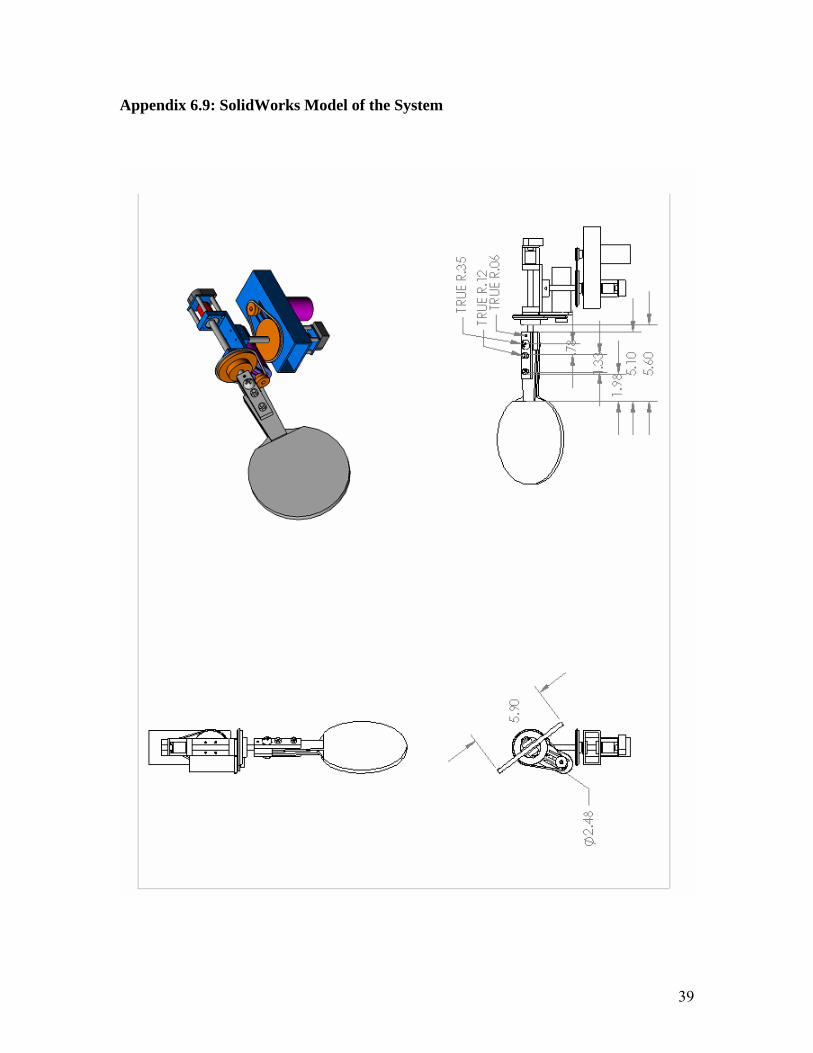
Appendix 6.9: SolidWorks Model of the System

39

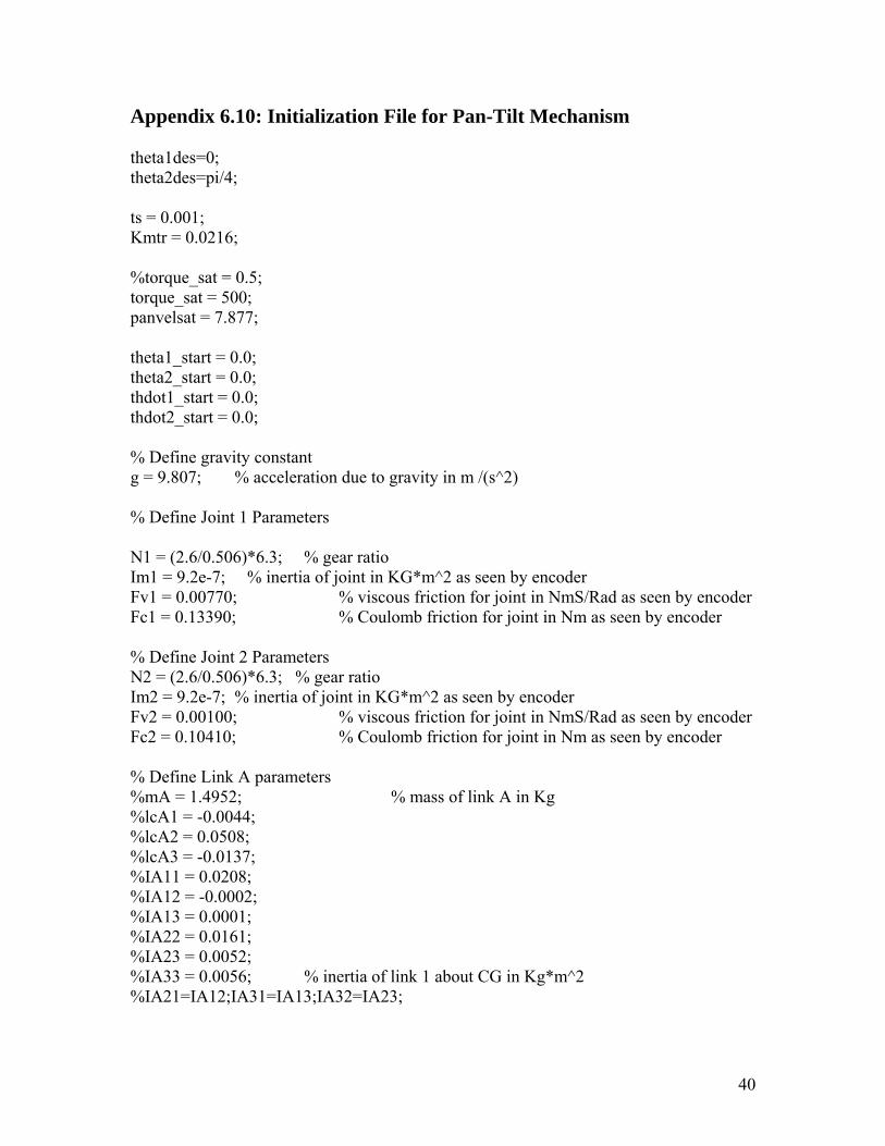
Appendix 6.10: Initialization File for Pan-Tilt Mechanism theta1des=0; theta2des=pi/4; ts = 0.001; Kmtr = 0.0216; %torque_sat = 0.5; torque_sat = 500; panvelsat = 7.877; theta1_start = 0.0; theta2_start = 0.0; thdot1_start = 0.0; thdot2_start = 0.0; % Define gravity constant g = 9.807; % acceleration due to gravity in m /(s^2) % Define Joint 1 Parameters N1 = (2.6/0.506)*6.3; % gear ratio Im1 = 9.2e-7; % inertia of joint in KG*m^2 as seen by encoder Fv1 = 0.00770; % viscous friction for joint in NmS/Rad as seen by encoder Fc1 = 0.13390; % Coulomb friction for joint in Nm as seen by encoder % Define Joint 2 Parameters N2 = (2.6/0.506)*6.3; % gear ratio Im2 = 9.2e-7; % inertia of joint in KG*m^2 as seen by encoder Fv2 = 0.00100; % viscous friction for joint in NmS/Rad as seen by encoder Fc2 = 0.10410; % Coulomb friction for joint in Nm as seen by encoder % Define Link A parameters %mA = 1.4952; % mass of link A in Kg %lcA1 = -0.0044; %lcA2 = 0.0508; %lcA3 = -0.0137; %IA11 = 0.0208; %IA12 = -0.0002; %IA13 = 0.0001; %IA22 = 0.0161; %IA23 = 0.0052; %IA33 = 0.0056; % inertia of link 1 about CG in Kg*m^2 %IA21=IA12;IA31=IA13;IA32=IA23;

40

% Define Link A parameters mA = 1.0656; % mass of link A in Kg lcA1 = -0.0062; lcA2 = 0.0254; lcA3 = -0.0598; IA11 = 0.0044; IA12 = -0.0003; IA13 = -0.0002; IA22 = 0.0021; IA23 = 0.0009; IA33 = 0.0029; % inertia of link 1 about CG in Kg*m^2 IA21=IA12;IA31=IA13;IA32=IA23; % Define Link B parameters mB = 0.4279; % mass of link B in Kg lcB1 = 0.0001; lcB2 = 0.1140; lcB3 = 0.1010; IB11 = 0.0061; IB12 = -0.0001; IB13 = 0.0; IB22 = 0.0060; IB23 = 0.0; IB33 = 0.0003; % inertia of link 1 about CG in Kg*m^2 IB21=IB12;IB31=IB13;IB32=IB23; % Design the controller kp1 = 2.0; kd1 = 1.0; ki1 = 0.1; p1 = 150; kp2 = 10.0; kd2 = 5.5; ki2 = 6.0; p2 = 150; %%%%%%%%%%%%%%%%%%%%%%%%%%%%%%%%%%%%% IN NATURAL STATE VARIABLE NAMES % % M11 % $$$ IA33+mA*lcA1^2+mA*lcA2^2+Im1*N1^2+IB11+mB*lcB2^2+mB*lcB3^2+(IB33+m

41

B*lcB1^2-IB11-mB*lcB3^2)*cos(u(1))^2+(-2.0*IB13+2.0*mB*lcB1*lcB3)*sin(u(1))*cos(u(1)) % $$$ % $$$ (-mB*lcB3^2-IB11+IB33+mB*lcB1^2)*c2^2 % $$$ +(-2*IB13+2*mB*lcB1*lcB3)*c2*s2 % $$$ +IA33+mA*lcA1^2+mA*lcA2^2+Im1*N1^2+IB11+mB*lcB2^2+mB*lcB3^2 % M12 % $$$ sin(u(1))*(-IB12+mB*lcB1*lcB2)+cos(u(1))*(IB23-mB*lcB2*lcB3) % $$$ % $$$ (-IB12+mB*lcB1*lcB2)*s2+c2*IB23-c2*mB*lcB2*lcB3 % M22 %IB22+mB*lcB1^2+mB*lcB3^2+Im2*N2^2; %IB22+mB*lcB1^2+mB*lcB3^2+Im2*N2^2 % Cdot1 % $$$ (2*IB11*c2*s2+2*mB*lcB3^2*c2*s2 % $$$ -4*c2^2*IB13+2*IB13 % $$$ +4*c2^2*mB*lcB1*lcB3 % $$$ -2*mB*lcB1*lcB3-2*c2*IB33*s2-2*c2*mB*lcB1^2*s2)*td2*td1 % $$$ +(-c2*IB12+c2*mB*lcB1*lcB2-s2*IB23+s2*mB*lcB2*lcB3)*td2^2 % $$$ % $$$ ((2.0*IB11*cos(u(1))*sin(u(1))+2.0*mB*lcB3*lcB3*cos(u(1))*sin(u(1))-4.0*cos(u(1))*cos(u(1))*IB13+2.0*IB13+4.0*cos(u(1))*cos(u(1))*mB*lcB1*lcB3-2.0*mB*lcB1*lcB3-2.0*cos(u(1))*IB33*sin(u(1))-2.0*cos(u(1))*mB*lcB1*lcB1*sin(u(1)))*u(2)+(-cos(u(1))*IB12+cos(u(1))*mB*lcB1*lcB2-sin(u(1))*IB23+sin(u(1))*mB*lcB2*lcB3)*u(3))*u(3)

42

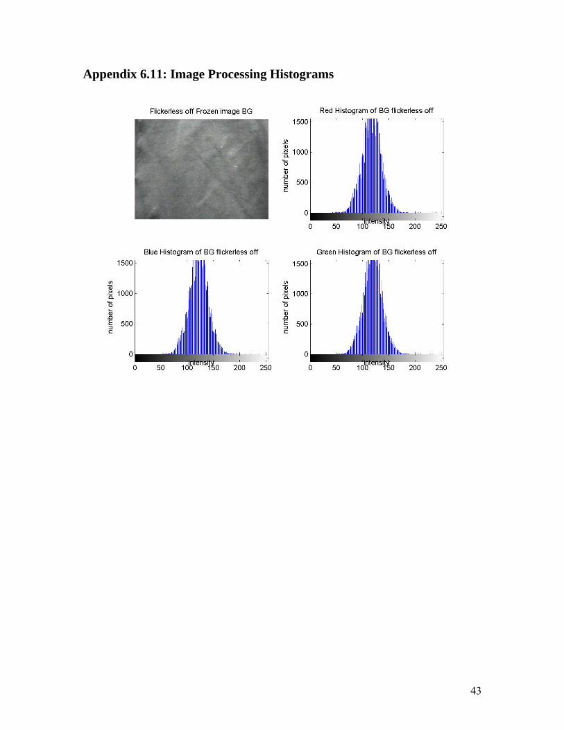
Appendix 6.11: Image Processing Histograms

43

44

45

46