I REPORT DOCUMENTATION _P

m ow ow.AD-A257 0401. AGENCY USE ONLY (Leave Bwar*) 2. REPORT DATE

August 1992

4. TITLE AND SUBTITLE 5. FUNDING NUMBERS

Automated Interpretation of Topographic Maps

6.AUTHOR(S)

Cronin, T. M.

7. PERFORMING ORGANIZATION NAME(S) AND ADORESS(ES) S. PERFCPIAING ORGANIZATIONREPORT NUMBER

U.S. Army CECOM Signals Warfare Directorate 92-TRF-0041Vint Hill Farms StationWarrenton, VA 22186-5100

9. SPONSORING/MONITORING AGENCY NAKIE(S) AND ADRESS(ES) JF A A10. SPONSORINGAMNITORING AGENCY

E EE REPORT NUMBER

SEP1 0 1992

SESI. SUPPLEMENTARY NOTES C

12a. DISTRIBUTIONWAVAILABILITY STATEMENT 12b. DISTRIBUTION CODE

Statement A: Approved for public release; distributionunlimited.

13. ABSTRACT (Mudmum20 wwrds) Some new results which impact favorably upon the issue of auto-

mated topographic map interpretation are presented. Actuilly, the "new" results consist

of heretofore undiscovered applications of two concepts known to mathematicians and

computer scientists for many years: binary search, and the normal vector. Binary search

is extended by the technique from not only one to two dimensions, but arguably to three

dimensions, since topographical maps are two-dimensional representations of three-

dimensional surfaces. Such maps are essentially sorted hierarchies of nested contours,

which form a muliply-connected subdivision of the plane. The perimeter of a subdivision

element is defined by a set of contours of extremal elevation and the edges of the map;

a naming convention attaches a label to each element of the planar subdivision. When-

ever one is afforded the luxury of dealing with a sorted data structure, one may invoke

the power of binary search to achieve O0log nItime complexity during processing of a

topographical query, where n is the number of contours which comprise a specific element

of the planar subdivision. A topographical query is a request by a user to interpret th

position of an arbitrary map coordinate, called query point, topographic map background.

1. SUBJECT TERMS 15. NUMBER OF PAGES

Artificial Intelligence, Applied Mathematics, Data Fusion, 21

Topographic Line Map (TLM) 16. PRICE CODE

17. SECURITY CLASSIFICATION 18. SECURITY CLASSIFICATION 1H. SECURITY CLASSIFICAI ION 20. LIMITATION or ABSTP'OF REPORT OF THIS PAGE OF ABSTRACTUNCLASSIFIED UNCLASSIFIED UNCLASSIFIED UL

PJSNl 7540 01-280-5500 "rr', 2 '1

I I I I I I I II I I I I i • .

GENERAL INSTRUCTIONS FOR COMPLETIUNG CSIiThe Report Documentation Page (RDP) is used in announcing and cataloging reports. It is imprortFntthat this information be consistent with the rest of the report, particularly the cover and title page.Instructions for filling in each block of the form follow. It is important to stay within the lines to meetoptical scanning requirements.

Block 1. Agany. I Ise Only (Leave bl"nk). Block 12a. Dtrihution/AvailarbiltatelCeaDenotes public availability or limitations. Cite

Block 2. Rep.rLDa1.P Full publication date any availability to the pu:blic. Enter additionalincluding day, month, and year, if available (e.g. limitations or special markings in all capitals1 Jan 88). Must cite at least the year. (e.g. NOFORN, REL, ITAR).

Block 3. Type of Repnrt ard Dates_.Gov_ecd.State whether report is interim, final, etc. Ifapplicable, enter inclusive report dates (e.g. 10 DOD See DoDD 5230.24, DistributionJun 87 - 30 Jun 88). Statements on Technical

Documents."Block 4. Title-and Subtitle. A title is taken from DOE - See authorities.the part of the report that provides the most NASA - See Handbook NHB 2200.2.meaningful and complete information. When a NTIS - Leave blank.report is prepared in more than one volume,repeat the primary title, add volume number,and include subtitle for the specific volume. On Block 12b. Distribution Cod.classified documents enter the titleclassification in parentheses. DOD - DOD - Leave blank.

Block 5. Euming-Numbem To include contract DOE - DOE - Enter DOE distribution categoriesand grant numbers; may include program from the Standard Distribution forelement number(s), project number(s), task Unclassified Scientific and Technicalnumber(s), and work unit number(s). Use the Reports.following labels: NASA - NASA - Leave blank.

NTIS - NTIS - Leave blank.

C - Contract PR - ProjectG - Grant TA - Task Block 13.Abstra..t, Include a brief (MaximurnPE - Program WU- Work Unit 200 words) factual summary of the most

Element Accession No. significant information contained in the report.

Block 6. Author(s). Name(s) of person(s)responsible for writing the report, performing Block 14. Subj~ccL.Trrn%. Keywords or phrasesthe research, or credited with the content of the identifying major subjects in the report.report. If editoi or compiler, this should followthe name(s). Block 15. NnberuLP_agqes, Enter the total

Block 7. P-fP.ormingOiganization Name(s) and number of pages.Address(ýs). Self -explanatory. Block 16. EncBCPAde. Enter appropriate price

Block 8. PerfomringOrganization Report code (NTIS only).Numnber. Enter the unique alphanumeric reportnumber(s) assigned by the organization Blocks 17. - 19. 5vurtyCns.iati.performing the report. Self-explanatory. Enter U.S. Secutity

Block 9. Spon,orinLMouitorin gAgieniy Classification in accordance with U.S. Securitymes,_and Addr . Self-explanatory. Regulations (i.e., UNCLASSIFIED). If formcontains classified information, stampBlock 10. SponsDringLMitoring Agfin classification on the top and bottom of the page.Report Number. (If known)

Block 11. Sipp]otes, Enter Block 20. Limftat[onotAbstract This blockBloc 11.,S~up~eo~tes, Etermust be completGd to a':sign a limitation to theinformation not included elsewhere such as:Prepared in cooperation w-ith...; Trans. of...; To abstract. Enter either UL (unlimited) or SARbe published in.... When a report is revised, (same as report). An entry in this block isInclude a statement whether the new report necessary if the abstract is to be lilmited. Ifsupersedes or supplements the older report. blank, the abstract is assumed to be unlimited.

C.- -A-A • •- . .

Ik Aceso Por-

' • -"• NTIS • "

Justti leat Gi..

Automated Interpretation of Topographic Maps D -•, r! bvt i or/

I Av~ilability Codes

T. Cronin AT

CECOM Signals Warfare Directorate -Dist 9pecialWarrenton VA 22186-5100

Abstract: Some new results which impact favorably upon the issue of automated topographic map interpretationare presented. Actually, the "new" results consist of heretofore undiscovered applications of two concepts known tomathematicians and computer scientists for many years: binary search, and the normal vector. Binary search isextended by the technique from not only one to two dimensions, but arguably to three dimensions, sincetopographical maps are two-dimensional representations of three-dimensional surfaces. Such maps are essentiallysorted hierarchies of nested contours, which form a multiply-connected subdivision of the plane. The perimeter of asubdivision element is defined by a set of contours of extremal elevation and the edges of the map; a namingconvention attaches a label to each element of the planar subdivision. Whenever one is afforded the luxury of dealingwith a sorted data structure, one may invoke the power of binary search to achieve O[ log n ] time complexity duringprocessing of a topographical query, where n is the number of contours which comprise a specific element of theplanar subdivision. A topographical query is a request by a user to interpret the position of an arbitrary mapcoordinate, called the query point, in the context of a topographic map background. An "interpretation" as currentlydefined consists of a five-tuple of information: the label of the map subdivision element within which the querypoint resides; the topographical contour of the subdivision element within which the point minimally resides; thelocal slope at the point; the local elevation at the point; and the flank of the partition element (hillside) upon whichthe point is situated. As an example, the following list is an interpretation of a query point: (Mt. Hood subdivision,contour #10600-d, 65 degree gradient, 10655 feet elevation, 350 deg NW). As is the case with one-dimensionalbinary search, the two-dimensional version must concern itself with items having identical keys. Becausetopographical maps may contain multiple contours lying at the same elevation, the topographical query processmust have a mechanism for choosing among "I =m before proceeding. Thus, when "halving the interval", one mustcheck to ensure that the interval is in fact uniquely def'ied. Inclusion testing within contours is achieved with adeterministic point-in-polygon algorithm developed by the Army in previous research. The traditional normal vectoris utilized extensively by the point-in-polygon algorithm, and also by the processing components which interpolateslope and elevation, and determine hillside emplacement. A new theorem derived from the law of cosines provides adecision rule based on integer arithmetic to decide which segments of a polygonal boundary justify a computation ofthe normal vector. As a byproduct of the research, an algorithm based on the Cevian formula has been developed tofind the nearest segment to a query point, without using any floating point operations whatsoever. Future researchissues include the topic of visual line-of-sight (binary map coloring) from a query point, and an analysis of the spaceand time complexity of the new technique, vs. the more burdensome alternative of storing elevation and slope data inlarge raster archives.

I. BACKGROUND AND TERMINOLOGY

Topographic Line Maps.

A topographic line map (TLM), also known as a contour map, is a vector representation of the boundariesof cross sections of the earth's surface. The projection of the boundary of a cross section of the earth's surface ontothe xy-plane is called a topographic contour. The equispacing between cross sections along the z axis is called thecontour interval of the map. A contour map is bounded by the rectangular edges of a map sheet. The edges of a map

92-24679~) V '~ III/IIfiIIIIIII 11 111111Iill)lll;ll!l

form what is called a clipping region, which prevents an observer from knowing the behavior of portions of contourswhich pass outside the rectangular perimeter of the map.

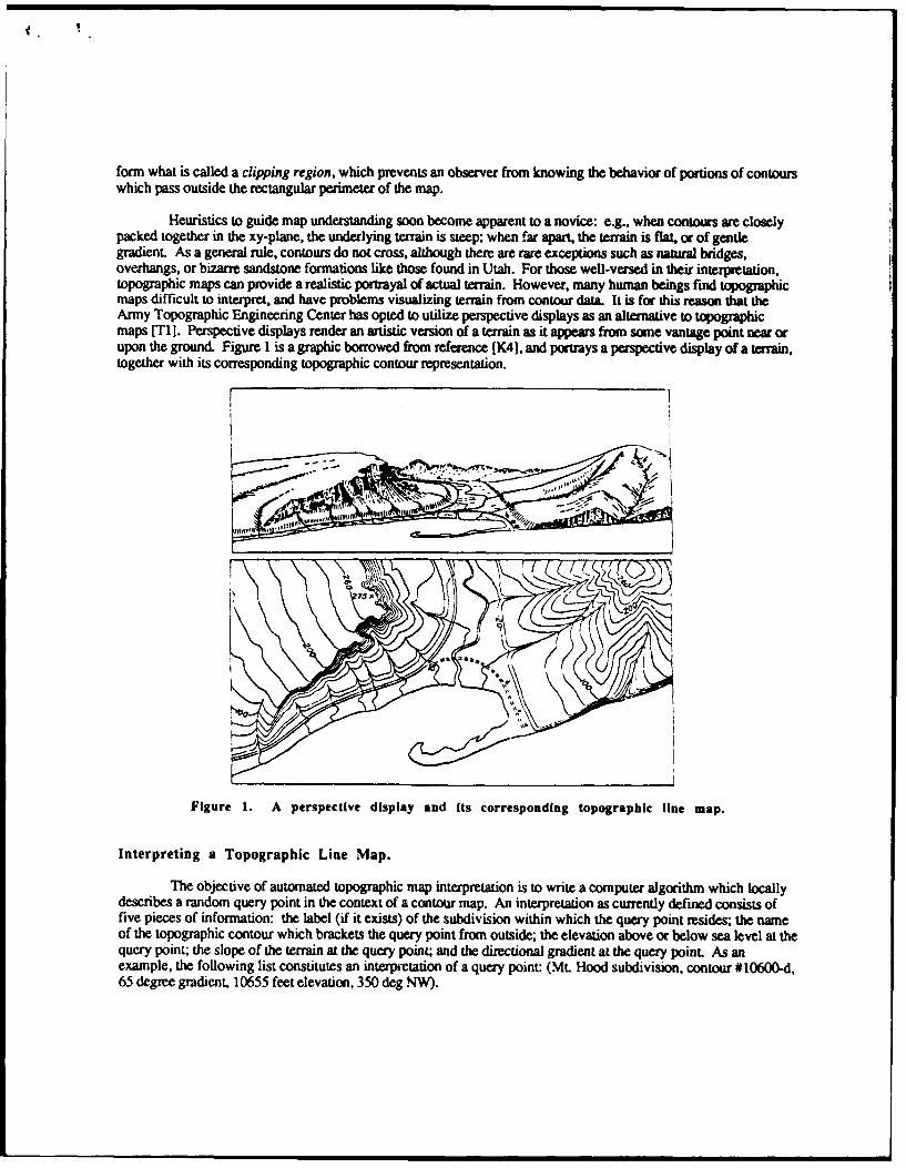
Heuristics to guide map understanding soon become apparent to a novice: e.g., when contours are closelypacked together in the xy-piane, the underlying terrain is steep; when far apart, the terrain is flat, or of gentlegradient. As a general rule, contours do not cross, although there are rare exceptions such as natural bridges.overhangs, or bizarre sandstone formations like those found in Utah. For those well-versed in their interpretation,topographic maps can provide a realistic portrayal of actual terrain. However, many human beings find topographicmaps difficult to interpret, and have problems visualizing terrain from contour data. It is for this reason that theArmy Topographic Engineering Center has opted to utilize perspective displays as an alternative to topographicmaps [Ti]. Perspective displays render an artistic version of a terrain as it appears from same vantage point near orupon the ground. Figure 1 is a graphic borrowed from reference [K41, and portrays a perspective display of a terrain,together with its corresponding topographic contour representation.

Figure 1. A perspective display and its corresponding topographic line map.

Interpreting a Topographic Line Map.

The objective of automated topographic map interpretation is to write a computer algorithm which locallydescribes a random query point in the context of a contour map. An interpretation as currently defined consists offive pieces of information: the label (if it exists) of the subdivision within which the query point resides; the nameof the topographic contour which brackets the query point from outside; the elevation above or below sea level at thequery point; the slope of the terrain at the query point; and the directional gradient at the query point. As anexample, the following list constitutes an interpietation of a query point: (Mt. Hood subdivision, contour #10600-d,65 degree gradient, 10655 feet elevation, 350 deg NW).

The five pieces of information currently sought by the algorithm hardly constitute a complete interpretationof a query point. Other descriptors are desirable in the long term: e.g., the visual line-of-sight from the query point,the profile of a traversible path passing through the query point, the profile of a path which optimally avoids thequery point. the feasibility of using the query point as a site for sensor placement, etc. However, the five primitivedata currently being returned by the algorithm go far toward providing inputs to some of the higher level queries,which may be synthetically constructed from the primitive queries.

Contour Notation.

In this section, notation is adopted to facilitate reasoning with topographic contours. Associated with everycontour is a specific value, denoted El(C), which represents the contour's elevation above or below sea level. Theelevation is modulo k, where k is the fixed contour interval of the topographic map. On a particular map, there maybe several distinct contours with the same elevation value; for spatial reasoning applications it is important todifferentiate among them. Each contour with an elevation value above sea level is contained within another contour,and may itself contain contours.

If contour C1 is contained within contour C2, then C1 is said to be nested within C2 . A contour cannot becontained within two or more contours which are not nested, but it can contain multiple contours which are notnested. If C is a contour of interest, then we denote the contour which minimally contains C to be C-. Byminimally contained, it is meant that any other contour D other than C- which contains C also contains C-, whichimplies that both C- and C are nested within D. A contour minimally contained by C is called C+, where the set ofall such contours is denoted {C+). If a query point lies between two elements of (C+), then it is said to be a saddlepoint. Note that {C+} may be the null set. A graphic illustrating these concepts is shown below.

Contour Notation: C, C-, and {C+}

Contour C+ is inside contour C, which is inside Contour C7.

c-+

{C+={ C+ 1 , C+2 , C+3

Figure 2. An illustration of contour containment.

A query point and its bracketing contours.

A query point is defined to be any random point of interest Except for special cases, a query point isbracketed by adjacent contours of a map: one contour which encloses it, called the outer bracket, and another contourwhich does not enclose it, called the inner bracket. Since contours are well-ordered at cluispaced elevations, thedifference in elevation between bracketing contours is equal to plus or minus the fixed contour interval of the map(except for a zero difference at saddle or culvert points). The figure below illustrates the brackets of a query point.

A Query Point and its Bracketing Contours

p =query point

C = outer bracket

C+ = inner bracket

Figure 3. Bracketing a query point from within and without.

II. TWO-DIMENSIONAL BINARY SEARCH APPLIED TO TOPOGRAPHIC MAPS.

Extending binary search to two dimensions to interpret topographic maps.

Binary search has traditionally been applied to a one-dimensional data structure, sorted by some user-definedordering property. The data structure might be an array of numbers sorted by the natural ordering of the reals, or alist of employee records sorted alphabetically by name. One commonly utilized data structure is 2D trees, in whichthe data consists of a set of ordered pairs of integers. In a 2D tree, the data is sorted on two keys (the abscissa andthe ordinate), with one key primary. A 2D tree is not a true instance of two dimensional binary search data structure,because one key is predominant over another during the sorting process. A better candidate is outlined at [K2], inwhich an interior point method for linear programming "halves" an ellipse during point-in-polygon testing.However, to be truly elegant, two dimensional binary search should avail itself of the natural containment propertyinherent to two dimensions. In the digital domain of the computer, two dimensional objects are in generalpolygons. Just as the one dimensional version must check to see if a point ties between two other points, the two-dimensional version is required to decide if a polygon is contained "between" two other polygons [C1]. Betweennessis equivalent to bracketing a query point with nested polygons.

Topographical contours exhibit a natural ordering due to the way in which the forces of nature havecombined to stabilize the crust of the earth. For example, gravity has assured that the top portion of a mountain has

a smaller cross section than its base. Thus, when projected onto a plane, contours from the same mountain appearto be nested. Ordering by elevation, and nesting by containment are properties which may be exploited to sortcontours. The data structure which results by appealing to a two-dimensional sort on elevation and nesting is calledthe contour containment graph. The motivation is that to exploit the O[ log n I query power of binary search, onerequires that the underlying data structure be sorted. We will see below that there are two preprocessing stepsrequired to set up an efficient two-dimensional search of topographic maps: the first is the construction of thecontour containment graph, and the second is the partitioning of the containment graph into regions suitably indexedfor binary search.

The Contour Containment Graph, and Labeling of Topographic Features.

As a first step in constructing the contour containment graph, we can uniquely label each contour, and thensort all contours on elevation, in ascending order. We then "nest" contours. To illustrate, suppose a specific 100-meter contour is labeled, and the contour interval of the map is 10 meters: we now seek to find all 110 metercontours contained within the labeled contour. If we find one, we create a pointer from the 100-meter contour's labelto the label of the 110 meter contour discovered to be contained in the contour. We continue this process until nomore contours are found to be within the 100-meter contour. We repeat this operation for all other 100-metercontours. When this step is completed, we switch our baseline cell complex from all those bounded by 100-metercontours to all those bounded by 1 10-meter contours, and continue the process until there am no contours remainingto be processed. An example of a terrain and its contour containment graph is depicted in the figure below. Theterrain features three hills. All three are contained within baseline contours of twenty and forty meters elevation.Note that a label may be associated with the forty meter contour to delimit the extent of the "hill country". Also, alabel may be installed on each of the sixty meter contours to name the individual hills. One of the three hillscontains two smAll knobs at the top, at an elevation of one hundred twenty meters. Each time that the set (C+)contains multiple elements for a given contour C, another level of sorting must be initiated to assure that thecontour containment graph is properly stra'tured and nested for binary search.

P •N

Binary Search .- Co tml r 26

Levd 1 Top Sort0

C r66(1) C.mig- 6)

Cm0 4 6(3)

Blonwy Search - Coffor U(1) Celr 52)

CIIS 5(3)C WO( C-()m " 1W(2)

C.omomr I(3)

Level 2 T opo Sort Cook o , 12() Cook e 1 2 2 Cooker 1 63)Cooker 1201(l) Cosior 12W2) C looke 126()

C m , ro o 1 4 1 ( 1 ) C .t tw 1 4 0 ( 2 )

Binary Search - Contou 12OX1) Cemlooi 124MLeAd 3 Top o Sort

Figure 4. A sorted terrain, nested In preparation for binary search.

Within each level of a contour containment graph, binary search may be invoked to achieve O[ log n I timecomplexity, where n is the number of contours contained at that level. To illustrate, in the figure below, a hill isrepresented by eight contours. On the first iteration of binary search, a contour halfway up the hillside at eightymeters is considered, and the query point is determined to be inside. On the second iteration, it is determined that thequery point is not inside the one hundred twenty meter contour, which is three quarters of the way up. The thirditeration decides that the point is not inside the one hundred meter contour, which is five eighths of the way to thetop. At the next iteration binary search concludes, having bracketed the query point between the eighty and onehundred meter contours, while having interrogated only three of the eight contours.

a - a contom' 2*

Is p inside 1O-Wner cnow? /- yes

Is P inside mi0nde Ca~omm?- No

Is p inside 100-inewe contolr?- •No

Number of contoum seched P

. 428=3 36

Conclusion: p is between an80-meter contour and a100-meter contour, at about 85meters altitude, on a moderateslope of about 30 degrees, whichfaces roughly northwest.

Figure 5. Binary search brackets a query point.

Although two-dimensional binary search may achieve O[ log n I time complexity over a database of ncontours, the issue remains open regarding the time complexity of the search as a function of the number of verticescontained within a given contour. For example, one topographic contour may contain a single vertex, whereasanother may contain thousands of vertices. Processing a set of contours comprised of a small number of vertices isclearly more desirable for performance consideratiors than processing a set of contours comprised of a large numberof vertices. An objective metric of time complexity should take into account both the number of contours and thenumber of vertices per contour.

Partitioning a Topographic Map for Binary Search.

Any topographical map contains contours of locally minimum elevation. These are readily identified fromthe contour containment graph developed in the preceding section. The strategy is to partition the map between allsuch contours, by constructing synthesized boundaries to act as cuts for binary search. Optimal placement of the cutboundaries is a load balancing problem, which needs to address not only the number of contours within each cut, butthe total number of vertices which comprise contours in the cut. In the diagram below, four hills have beenpartitioned by synthesized boundaries into regions suitable for binary search. Note that the bold lines are notcontours but synthetic boundaries. The first cut runs roughly down the middle of the map, and segregates therightmost hill from the other three. Observe that the first cut contains nine contours on the left, but only seven onthe right. This is not arbitrary, but is designed to compensate for the longer perimeters of the contours on the rightof the cut (it is implied that a longer perimeter equates to a larger number of vertices in the contour boundary data).

The second cut is dependent upon the decision made during the fitr cuL If a query point is to the left of the fiur cut,then the second cut lies between the two most northerly hills and the hill in the southwest corner. Conversely, ifthe query point is to the right of the first cut, then the second cut lies halfway up the rightmost hill. Continuing inthis fashion, the number three cuts are synthesized. No further cuts are shown, but the logic to create them issimilar.

Partitioning a Contour Map for Binary Search<=>312

Bold lines are synthesized for • "• "•ibinary search.

Figure 6. Load balancing a contour map to create a two-dimensional binary tree.

Dealing with contours which exit the clipping region of a map.

Figure 6 is oversimplified. In gencial, contours are not so well-behaved. There is one common problem toconsider a contour may exit the rectangular region bounding the map, and therefore pass outside the clippingregion. The problem may be solved by conjoining the troublesome contour with the rectangular edge of the map.This contrivance forces two polygons to be synthesized from the errant contour, to create a data structure compliantwith two-dimensional binary search. Synthetic boundaries for binary search may also be constructed accordingly.

The figure below depicts a clipped contour of forty meter elevation which exits the map at both sides. Twodimensional binary search requires that data structures be in the form of polygons. We synthetically create two newpolygons by conjoining the clipped contour with the edges of the map. Because the point-in-polygon algorithm ofchoice (described in the next section) requires a sense of handedness, we assure that the vertices of the new polygonsare in counterclockwise order. At execution time, we may now ask if a query point is contained within either theupper or the lower polygon manufactured by utilizing the clipped contour, and proceed accordingly.

ClippingRegion 4

40

Figure 7. Creating two polygons from a clipped contour.

III. AN INCLUSION (POINT-IN-POLYGON) ALGORITHM, AND PROXIMITY.

Perceived shortcomings of currently available point-in-polygon technology.

The two-dimensional binary search algorithm requires a utility function to establish whether or not a querypoint is inside a topographical contour. The utility function is a true workhorse, so it must be efficient. There isno margin for error, which means that point-in-polygon algorithms which rely on the precision of machinearithmetic are inappropriate candidates. For this reason, approaches based on the winding number or the parityalgorithm are currently infeasible. The Apple Macintosh family of computers has implemented a predicate called"point-in-region-p", available as part of the Quickdraw graphics repertoire, but the predicate consumes quadraticamounts of region space in memory, which becomes prohibitive for even a moderate number of polygonalboundaries. A high-performance algorithm from the computational geometry literature, based on triangulation [K3],is a viable candidate, although it remains an untested quantity, since it has never been tasked against a multi-megabyte database of topographical contours.

Because of perceived shortcomings of on-the-shelf point-in-polygon algorithms, and the lack of benchmarkdata to test the performance of the triangulation algorithm, the author has opted to implement his own algorithm[C2], which has been extensively tested against actual contour data. The algorithm assures that a contour is orientedin a counterclockwise direction, so that the interior of the contour is to the left during traversal. Inclusion testing isthen conducted as a function of a query poinfts proximity to a contour (see figure below). One benefit of thealgorithm is that it returns distance and direction (normal vector) to the nearest point on a boundary, in addition tothe inclusion decision. As will be seen below, the normal vector is crucial to topographic map interpretation. Asoriginally conceptualized, the algorithm anticipated that every pixel in a digital boundary would be explicitlyavailable as part of the data structure. However, the Defense Mapping Agency does not represent feature boundariesso obviously. Instead, a contour is provided in chain-coded format, where the boundary of the contour consists of aset of ordered vertices. It is up to the user of the data to create the edges which join the vertices.

Proximity and Inclusion of a Query Point p to

Contour C

e 0. C is a set of chain-coded verticeswith implied edges.

t 1. Order C counterclockwise.ccw1

2. Selectively drop normal n to C.

3. If magnitude of n < magnitude ofall other normals, then p is closestto edge e of contour C.

4. If p is to the right of C, it isoutside; otherwise it is inside.

Figure S. The normal vector may be used to decide Inclusion.

The Voronoi diagram for data produced by the Defense Mapping Agency.

Vector data distributed by the Defense Mapping Agency (DMA) contains three kinds of objects: points,line segments, and polygons. It has been known for some time that the skeleton, or medial axis of a polygonconsists of portions of parabolas and line segments [12]. The parabolas are the locus of equal distance betweenpoints and segments. The line segments are the locus (angle bisectors) between extended segments. It is also truethat for any set of points, segments, and polygons the equidistance locus consists of parabolas and line segments.Thus, the Voronoi diagram for DMA data, which is defined to be the locus of equal distance, is in general parabolic.

There is currently no commercial product available to generate the parabolic Voronoi diagram for anarbitrary set of polygons, segments, and points. However, there are three research and development tools (of varyingdegrees of robustness) circulating among researchers -T, academia [M31. The developmental products implemented todate have encountered problems of numerical precision, primarily when deciding upon which side of a parabola aquery point lies [F21. However, as indicated at reference [El], the theory behind the sweepline algorithm [Fl] togenerate the linear Voronoi diagram should be directly extensible to the parabolic diagram. It is clear that for theasymptotic solution to the static proximity problem, the Voronoi diagram is the paradigm of choice. As a stopgapmeasure, until a tool to generate the parabolic diagram is available, the author has developed his own proximityalgorithm, described below, based on restricted use of the normal vector. The author's algorithm, unlike the Voronoidiagram, facilitates dynamic objects. If an object's position changes, the Voronoi diagram must reinvoke a relativelyexpensive preprocessing step, whereas the author's algorithm simply replaces the object's old boundary position withthe new.

Finding the nearest point of a contour to a query point.

A contour, which when represented with digital data is in the form of a polygon, consists of a set ofvertices and the implied edges which connect the vertices. Thus, when one speaks of proximity to a contour from aquery point, one is actually referring to minimal Euclidean distance to the set of vertices, vs. distance to the set ofedges.

Minimal distance to an edge is non-trivial to compute. This process entails dropping the normal vectorfrom a query point to the edge. Since floating point operations may be required at every edge to which the normal isdropped (although the author introduces below a new technique which avoids floating point arithmetic), we wouldlike to limit the number of edges incurring such an expensive operation. If the normal vector strikes an edgedirectly, the edge is said to be admissible to the normal vector. Refer to the figure below. Clearly, it does notbehoove us to drop the normal from query point p to edge e2, since the tip of the normal does not even inte, sect e2,but rather its extension. Such cases are precisely those which we strive to avoid, by appealing to a normal vectoradmissibility filtering technique. It will be shown below that as a side effect, the filtering technique returns minimaldistance to a vertex.

Normal Vector Admissibility

e 1 is admissible;P n2e 2 is not

n, e,Contour boundary e3el - e2- e3 . . .

Figure 9. Certain contour edges do not admit the normal vector.

Derivation of edge admissibility conditions from the law of cosines.

Construct orthogonal rays from the endpoints of contour edge e, as in Figure 10 below. Now suppose thatquery point p lies between the rays. Note that the angle between edges x and e is acute, as is the angle betweenedges y and e. Let the angle between y and e be 01 and the angle between x and e be 02. Then, by the law ofcosines,

x2 = y2 + e2 -2 y e cos 01 [1]y2 = x2 + e2 -2 x e cos 02 [2]

The cosine function is positive for acute angles. We therefore obtain

x2 + al = y2 + e2 [3]

y2 + a2 = x2 2 + e2 ; cl, a2 >0 [4]

These equations are alternatively expressed by the inequalities:

x2 < y2 +e 2 [51

y2 < x2 +e 2 [6]

This set of inequalities must be true for segment e to admit the normal vector. Point p of Figure 10 satisfies theconditions.

Admissible Normal Vector Condition

Both base angles are acute.

p

n

e = segment of boundary

Figure 10. An edge is admissible If base angles are both acute.

In practice, it is more likely for the test to be failed than to be passed, so it makes sense to test first for

failure rather than for success. The failure condition may be written as the predicate

.. [ x2 < y2 +e 2 A y2< x2 +e 2 ] [71

From DeMorgan's rules, this may be rewritten

-'[x 2 <_ y2 +e 2 ] v _[y2<_ x2 +e 2 ] 181

which is equivalent to

x2 > y2 +e 2 v y2 > x2 +e 2 [91

If either side of disjunction [9] is true, then edge e is not admissible to the normal vector, and a potentiallyexpensive floating point operation is avoided by means of a simple integer-valued decision function. An example ofsatisfaction of the second inequality of the disjunction is illustrated at the figure below. In this case, edge e fails theadmissibility condition, so that the normal vector computation is avoided.

Inadmissible ConditionA base angle is obtuse.

p ,_ __ _

nY

e = segment of boundary

Figure 11. An obtuse base angle precludes admissibility.

As a byproduct of the admissibility test, minimal distance to a vertex is returned. Consider the integer-valued expression (Sp-Sv) 2

+ (tp-tv) 2, where (sv,t,) is the coordinate at the vertex and (sp,tp) is the coordinate at thequery point. This expression is synonymous with either of the arguments x2 or y2 in equations [1]-[91 above.Hence, the filtering operation as a side effect monitors the squares of the distances to each of the vertices of acontour. When the smallest such expression is found across all vertex possibilities, the square root is extracted. Theentire process involves n integer-valued operations for n vertices, and one floating point operation, for a timecomplexity of O[ n ]. The integer-valued operation here involves two integer multiplies, three integer adds, and aninteger comparison. The floating point operation is a single-shot appeal to the square root of the minimal integer-valued result.

A Common Lisp unplementation of the edge admissibility test might appear as follows:

(defun admissible-normal-segment-p (x y ak ay b, by)(a,, ay) and (b,, by) are the endpoints of segment e in figures; (x,y) is query point.

(prog (dislsqr dis2sqr dis3sqr)(declare (type longint x y ak ay b, by dislsqr dis2sqr dis3sqr))dislsqr = (dissqr a. ay b1 by)dis2sqr = (dissqr x y ak ay)dis3sqr = (dissqr x y b1 by)(cond ((> dis3sqr (+ dislsqr dis2sqr))(return nil))

((> dis2sqr (+ dislsqr dis3sqr))(return nil))(t (return t)))))

Finding the normal vector with minimum magnitude, across all segments.

Although we now have a test to determine which segments of a boundary admit the normal vector from aquery point, we have not said anything about the actual computation of the minimal such vector across all segments.In this section we develop a new test to find the smallest normal vector, without resorting to any floating pointcomputations. If the actual magnitude is desired, two floating point operations are required over the entire database.We appeal to a very useful result from analytic geometry, called the Cevian formula (for a development see [K I]). Acevian is defined to be a line segment drawn from a vertex of a triangle to the opposite side. Note that medians,angle bisectors, and altitudes are all examples of cevians. The Cevian formula is shown in the figure below, where nis an altitude in this case. It is convenient that the altitude is equivalent to the normal vector under discussion. Inthe figure, observe that rz and sz are lengths which sum to side z, whereas r and s are ratios which sum to one.

The Cevian Formula

InI 2 = ry2+sx 2-rsz 2,where r = rz/z and s =sz/ z

p

n

rz Sz

z = segment of boundary

Figure 12. The Cevian formula relates a normal vector to the sides of a triangle.

Unfortunately, we do not know the values of r and s, because we do not know the point at which thenormal vector impacts side z. In the equations below, which until step [15] echo the discussion in [KI], we derive aformula for the square of the magnitude of the normal in terms of a ratio involving the squares of the sides. Steps[101-111 are a reiteration of the information conveyed by the figure. Steps [121-[13] involve a substitution for s,followed by a reformulation as a quadratic equation in terms of r. In step [14] we set the discriminant equal to zero,because the roots of equation [13] must be non-negative and equal, since r and s form a convex set. Solving thisequation for n2 results in the ratio shown at [15], which but for the divide operation is economical to compute, sinceit involves four integer multiplies and three adds. If one were tuning the technique with assembly code, two of themultiplies (those involving the 4) could be converted into two-bit left shifts, since shifts are cheaper than multiplies.

r= -- ;s= L-; r+ssl; r1 +s,=z [10]Z z

n2 = 2 + Sx2 - rsz2 [111

n2 = ry2 + (I - r)x2 - r1 - r)z2 [121z 2 r2 -- (X2 +1 Z2 _ y2 )r + (X2 _ n•2) = 0 (13]

(Z 2 -y2 X2)2 - 4Z 2 (X 2 - n 2 ) = 0 [141

n2 4x2 - (x 2 + z 2 - y 2 ) 2 [15]

4z2

What about the division by 4z2 , which implies a floating point operation? The answer is that in order tofind the normal vector of smallest magnitude, we may refrain from performing the division until all admissiblesegments have been associated with a numerator and denominator as at [151, and checked against the shortest normalvector found thus far. The check is made as follows. Let n1 be the normal dropped from a query point to segmentz1 , with x1 and yj the distances to the respective endpoints of zl. Let n2, z2 , x2, and Y2 be defined similarly. Thenthe squares of the normals are shown respectively at [16] and [17]. Now n1 < n2 if and only if [19] and [201 are true,but [20] is true if and only if the product of the means is less than the product of the extremes as shown at [21].Cancelling the common factor produces test inequality [22]. Notice that if we are using integer-valued coordinates,as we must if we are working with data displayed to a computer screen, there are no floating point expressionsinvolved in the test.

z 4 z2 2 (2 .z2 - 2)22= 4x- - (XI + -iY [161

4z

2 4x2z2 - (x2 +4 Z2 _ y) 2

42 2 [171

n, < n2 It [18]

nt n2 4* [19]422 X2+Z2 22 4X2Z2 -(X2 2)2

4 1-(x+ -Y) < 2 Y2 [204Z2 44Z4 X2Z2 (X2 2 2)214Z2 <[x2z2 _2(x +.z2 _2)2 Z

[4x -(x +z - 14 2 < ([4 2 2-2 - ]4z (211

z[4x2z2 -(x2 + Z2 _ Z[44 _ (X2 + - _ [2212 [221 1 22 2

Using the test is simple. As input we receive a query point and candidate segment with integer coordinates.The squares of the distances from the query point to the segment endpoints are computed with the usual Euclideanformula, as is the square of the distance between the endpoints. These three quantities are used to compute theinteger-valued numerator and denominator of equation [15]. The same technique applied to some other candidatesegmen~t produces another numerator and denominator, which we cross-multiply with the first at inequality [221. Ifthe product of the means is less than that of the extremes, then the first segment is closer to the query point;otherwise the second segment is closer. We continue this process until all segments are exhausted, remembering thesegment giving rise to the shortest normal vector as we do so.

Observe that we have located the nearest segment (according to the true Euclidean metric) to a query pointwithout resorting to any floating point arithmetic. Granted, we do not yet know the magnitude of the shortestnormal vector, but we know that we have the shortest. To obtain the magnitude, we merely need to perform thedivision indicated at equation [15], and extract the square root of the result. Note also that we never had to computeany of the points of a line segment; we were able to make do with the vertices at its endpoints. This latter artifactdemonstrates the power and leverage of the Cevian formula, developed over three centuries ago. The formula maypotentially be used to assist in the generation of the parabolic Voronoi diagram for line segments and polygons.

We briefly summarize before moving on to the next section. When the two-dimensional binary searchparadigm reauests the inclusion algorithm to decide whether or not a query point is contained within a specificcontour, the inclusion algorithm is handed the counterclockwise-oriented set of contour vertices and the query pointas arguments. The first action taken by the inclusion algorithm is to subject all of the implied edges of the contourto the normal vector admissibility test, maintaining the squared distances to the vertices on the side. Generally, thetest returns just a handful of edges admissible to the normal vector. To each of these, the cross-product test shown at[22] is performed to locate the minimal normal vector. This quantity is compared against the minimal resultobtained for the vertices. If the square of the distance to an edge is smaller than the squared distance to a vertex, atest is invoked to decide if the query point is to the left or the right of the edge; if to the left, the point is inside thecontour, and if to the right, the point is outside. At this time the numerator and denominator of equation (15] maybe divided and the square root extracted to obtain the actual magnitude of the normal vector. If the squared distance toa vertex is smaller than that to an edge, a synthetic edge is constructed from the vertex's predecessor and successorvertices in the contour boundary, and a test is invoked to decide if the vertex is to the left or the right of thesynthetic edge; if to the left, the query point is inside the contour, and if to the right, the point is outside. Thesquare root may be extracted to obtain the magnitude of the normal vector. The shortest normal vector points toeither the inner or the outer bracketing contour of the query point.

IV. INTERPRETATION OF A QUERY POINT IN THE CONTEXT OF A MAP.

Binary search of a contour containment graph concludes by returning the two bracketing contours of a querypoint. The algorithm is now armed with all the information it requires to produce an "interpretation" of a querypoint, as defined in the first section of the paper. If either bracket has inherited the name of a mountain, hillside,crater, etc., for which the bracket is a structural element, then the name is available for simple display, or for furtherspatial reasoning operations such as line-of-sight or traversibility reasoning. Because inclusion testing as describedabove returns as a byproduct the normal vector from a query point to a contour, both the distance to the outer bracketand the distance to the inner bracket are known when binary search completes. These two distances may be used inconjunction with the contour interval of the map to obtain estimates for the point's elevation and slope. Thedirection from a hilltop to the query point, together with the elevation values and orientation of the bracketingcontours, may be used to determine a directional gradient, which establishes upon which flank of a hillside a querypoint resides. The details involved in extracting the elevation, the slope, and the directional gradient are describedbelow.

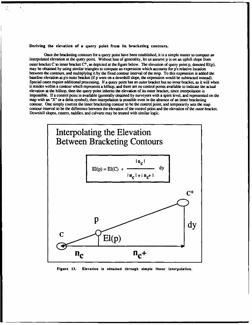
Deriving the elevation of a query point from its bracketing contours.

Once the bracketing contours for a query point have been established, it is a simple matter to compute aninterpolated elevation at the query point. Without loss of generality, let us assume p is on an uphill slope fromouter bracket C to inner bracket C+, as depicted at the figure below. The elevation of query point p, denoted El(p),may be obtained by using similar triangles to compute an expression which accounts for p's relative locationbetween the contours, and multiplying it by the fixed contour interval of the map. To this expression is added thebaseline elevation at ps outer bracket (if p were on a downhill slope, the expression would be subtracted instead).Special cases require additional processing. If a query point has an outer bracket but no inner bracket, as it will whenit resides within a contour which represents a hilltop, and there are no control points available to indicate the actualelevation at the hilltop, then the query point inherits the elevation of its outer bracket, since interpolation isimpossible. If a control point is available (generally obtained by surveyors with a spirit level, and represented on themap with an "X" or a delta symbol), then interpolation is possible even in the absence of an inner bracketingcontour. One simply coerces the inner bracketing contour to be the control point, and temporarily sets the mapcontour interval to be the difference between the elevation of the control point and the elevation of the outer bracket.Downhill slopes, craters, saddles, and culverts may be treated with similar logic.

Interpolating the ElevationBetween Bracketing Contours

In¢1

El(p) = El(C) + dy

C+

p dC El(p)

nc nc+

Figure 13. Elevation is obtained through simple linear Interpolation.

Obtaining the slope at a query point from its bracketing contours.

The local slope at a query point is so simple to estimate that even interpolation is not required. It issimply the angle with a tangent equal to "the rise over the run". The "rise" is fixed, as it is given by the contourinterval of the map. The "run" is defined to be the sum of the magnitudes of the normal vectors drawn to the outerand inner bracketing contours. At the top of a hill or at the base of a depression, in a saddle or a culvert, the slope isassumed to be zero, for flat ground. However, if a control point is available to provide additional elevation data, thenlogic similar to that outlined for elevation in the paragraph above may be utilized to obtain a refined estimate ofslope. Outside the limits of the lowest lying contours, the algorithm is designed to return the string "drainage area",which again is assumed to be flat ground. There may or may not be a perennial stream flowing through a drainagearea, but during flashfloods it is assumed that water would flow there.

Note that a peculiar thing happens if we slide the query point along either of the normal vectors pointing tothe bracketing contours. The slope remains fixed as we do so. This is the price we pay for approximating a terrainby a set of cross-sectional contours. The computed slope cannot be made more accurate than the resolution imposedby the contour interval of the map. Thus, between any two nested contours, there is a vector field of slope vectorswhich connect every digital point of the inner bracket with some digital point of the outer bracket, and vice versa.

Computing the SlopeBetween Bracketing Contours

Slope = arctan [ dy / dx ]

dy is given by the contour interval

C+

S~dy = 10 meters

... "' nc+-- 4

C

I dx=Inc I+ Inc+ I

Figure 14. The "rise" is fixed, and the "run" is the sum of the normal vector magnitudes.

Obtaining the directional gradient at a query point from its bracketing contours.

Again, assume the familiar example of an uphill slope, so that El(C) = El(C+) - k, where k is the fixedcontour interval of the map. Construct the vector from the hilltop to the query point. Define the hilltop to be thecontrol point at the top of the hill if it exists; otherwise make it some reasonable estimate, such as the centroid ofthe topmost contour. If there are multiple topmost contours, then make the hilltop the centroid of them all.Suppose that the hilltop to query point vector points to the left, as in the figure below. Then it is pointingdownhill, because C's elevation is less at that of C+, and it is pointing to the west, since due north is as shown bythe map. The query point is therefore on the western flank of a hillside. Variations on this theme are computablefor other configurations of terrain. If the elevation of C is greater than that of C+, and we observe a leftward-pointing vector, then we would be on the western flank of a crater or valley. If the elevation of C was to be equal tothat of C+ and the vector was to point to the south, then the query point would be on a saddle or in a culvert,oriented in an east-west fashion.

The vector pointing from a hilltop to a query point is a suitable gauge of directional gradient from a globalperspective. However, a query point may be situated locally on a geologic feature of a hillside, with an orientationseemingly at odds with the global result. For example, on the south side of a mountain, there may be a ridge whichproceeds from the summit down to the south. The ridge will have both eastern and western flanks. Suppose for thesake of argument that a query point is on the western flank of the ridge. We conclude it is possible for a query pointto be locally on a western flank, but globally on the south side of the mountain. The local flank estimate is easilycomputed by drawing the normal vector from the query point to its outer bracketing contour. The vector points inthe compass direction of the local gradient. This procedure is particularly useful for rugged terrain such as thatencountered on Mount Rainier in the state of Washington, where contour data tends to resemble a set of nested"octopuses".

Computing the DirectionalGradient on Hillsides

Magnetic north is given by map.

",,N

C+C

P

P is on a western flank of moderate gradient.

Figure 15. Determining a query point's emplacement on a hillside.

V. AN IMPLEMENTATION, AND CONCLUSIONS.

The theory of automated topographic map interpretation, as developed to date, has been partiallyimplemented on a Macintosh IIfx workstation, using Macintosh Common Lisp, version 2.0. There are plans toconvert the code into C, using the Symantec Think C environment. The conversion is intended not so much forperformance purposes, since the Lisp compilers performance is favorable when compared to that of the Symantecpackage, but to be able to control the process of garbage collection, which in the Lisp package is beyond the reach ofthe user.

There are two databanks of contour data. real and simulated. The first source of the real variety is a set ofdigital elevation matrix (DEM) data, which is a gridded representation of elevation values sampled at equispaced x andy increments. DEM data is produced by the United States Geographical Survey (USGS) office, as a result of datacollection performed primarily by civilian engineers. To obtain topographical contours from DEM data, one mayutilize a geographic information system (GIS) to extract contiguous points of equal elevation from the grid. Theauthor used an on-the-shelf GIS package called Macgrizo [MI] to create contours for the Killeen Texas area. Thesecond source of real data, which is the military counterpart to DEM data, is digital terrain elevation data (DTED),which currently is available in two resolutions: Level I, at 100 meter spacing, and Level II, at 30 meter spacing.

The simulated data is handcrafted by appealing to Macintosh Quickdraw graphics. A representative &erraincontaining four hillsides is depicted in the figure on the next page, where a query point is represented by the tip ofthe cursor (the arrowhead at the right). In this case, the partitioning algorithm during a preprocessing step createdlevel one and level two cuts to segregate the four hillsides. The level three cuts and beyond partitioned each of theindividual hills, using the nesting principle described earlier. Now comes execution time, and two-dimensionalbinary search. In this example, hills two and four were selected in the first binary cut, and hill two in the secondcut. In the third cut, it was determined that the query point was not inside hill two's forty meter contour, in thefourth cut it was determined that the point was inside the twenty meter contour. Binary search concludes at this timebecause the contour containment graph has been exhausted. Therefore, the outer bracket is hill two's twenty metercontour, and the inner bracket is the forty meter contour. Associated with each of these two contours is the label"HILL2". The gradient computation deduces an easterly downhill slope; the slope is computed to be forty eightdegrees; and the elevation interpolates to thirty three meters. Currently, the interpretation process says nothingabout the relationship among HILL2 and the other hills; future work will address this issue.

Future Work.

The research to date has focused on a local interpretation of a query point. By definition, a localinterpretation is limited to a description of a query point in terms of the label of the hill upon which it resides, thetwo contours which bracket it, an interpolated elevation, a slope value, and a directional gradient. This informationis useful for localized reasoning about the immediate environs of a query point. A natural outgrowth of this work isto extend the reasoning to a more global capability. For example, one could utilize knowledge about the location ofa hillside with respect to other hillsides in a specific region, to achieve context-cued line of sight reasoning ortraversibility planning.

To illustrate line-of-sight reasoning, consider the following example, based on the author's personalexperience. In Grand Teton National Park in Wyoming, if one is on the western shore of Jenny Lake, the tallestvisible peak is Teewinot Mountain, which looms spectacularly nearly a mile above the observer's head. One peakaway is the Grand Teton, which although a thousand feet higher, may not even be seen from this vantage pointbecause it is blocked from sight by Teewinot. The interpretation process described in Section IV would determinethat the query point is on the eastern flank of Teewinot Mountain, on a moderate slope, at about 6600 feet elevation.Utilization of the directional gradient calculation would indicate that the direction to the tops of Teewinot and theGrand Teton are roughly the same, but the slope of the segment joining the query point to the top of Teewinot isgreater than that drawn to the top of the Grand Teton. Hence, one concludes that line-of-sight westward to the Grand

is restricted by the intervening mass of Teewinot. Future work will involve refining and formalizing concepts suchas these.

Already, the normal vector admissibility filMeting technique has been extended to objects other thantopographic contours. The Defense Mapping Agency produces a set of vector overlays corresponding to atransportation network, a hydrology network, obstacles, surface orientation, surface composition, and vegetationtype. In additit,, the DMA produces a gridded product called digital terrain elevation data (DTED), at both thirty andone hundred meter horizontal resolution. The vector products together with thirty-meter DTED in large partcomprise what is known as tactical terrain data (CTD), a database being developed by DMA with the cooperation ofthe US Army Topographic Engineering Center (M21. The integer-based decision rule derived from the law of cosineshas proven to be of high utility in gauging proximity and inclusion with respect to the multi-megabyte vectordatabases contained in TTD.

Global location: HILL2

Flank of hill: EASTSlope in degrees = 48Elevation in merers = 33

Figure 16. Interpreting a query point in terrain.

'4

Conclusions.

Two-dimensional binary search has been utilized in conjunction with two new algorithms which avoid theexpensive floating point operations associated with computing the normal vector, to produce an algorithm adept atlocally interpreting topographic line maps. An interpretation consists of a human-like description of a query pointin terms of its global location, interpolated elevation, local slope, and directional gradient. The search algorithmrelies heavily upon proximity and inclusion algorithms developed with computational geometry research funded bythe US Army. For credibility, the technique is being leveraged against multi-megabyte databases of contourinformation corresponding to actual terrain. An integer-based decision function which arbitrates when to drop thenormal vector to an edge (during proximity testing) has proven to be extensible to objects other than elevationcontours, such as segments of roads and streams, and polygons delimiting types of vegetation cover and surfacematerial composition. As a byproduct of the research, an algorithm based on the ancient Cevian formula has beendeveloped to find the nearest segment to a query point, without using any floating point operations whatsoever.New work will focus on extending the definition of map interpretation to be more globally descriptive of a terrain.

Bibliography

[B1I Bentley, J., Programmng. Pearls, Addison-Wesley Publishing Company, Reading MA, 1986.

[1B2] Blum, H., A Transformation for Extracting New Descriptors of Shape, in Symp. Models for Perception of Speech andVisual Form, MIT Press, 1967.

[C11 Cronin, T., Topographical Contour Betweenness Testing, US Arnmy Signals Warfare Center Technical Report CSW-88-7. 1988.

[C2] Cronin, T., Optimized Annulus-based Point-in-Polygon Inclusion Testing for d Dimensions. Transactions of the

Seventh Army Conference on Applied Mathematics and Computing, West Point NY, 1989.

[Ell Edelsbrunner, H., Algorithms in Combinatorial Geometry Springer-Verlag, Berlin Germany. 1987.

[F1] Fortune, S., A Sweepline Algorithm tor Voronoi Diagrams, Proceedings of the Second Annual ACM ComputationalGeometry Symposium, 1986.

[F2] Fortune, S., private communication, AT&T Bell Laboratories. March 1992.

[KI] Kay, D., Collee Geometry. Holt, Rinehart, and Winston, Inc., New York NY, 1969.

[K21 Khachiyan, L.G., A Polynomial Algorithm in Linear Programming, Soviet Math. Dokl., Vol 20, No.1, 1979.

[K3] Kirkpatrick, D.G., Optimal Search in Planar Subdivisions, SIAM J. Comp. 12, 1983.

[K4] Kjellstrom, B., Be Expert with Map and Compass. rev. ed., Charles Scribner's Sons, New York NY, 1967.

[Ml] Macsridzo: The Contour Mamning Program for the Macintosh. Users Manual for Version 3, Rockware Inc., WheatRidge CO, 1990.

(M21 Messmore, J. and L. Fatale, Phase I Tactical Terrain Data (TTD) Prototvo Evaluation' US Army EngineerTopojgraphic Laboratories Technical Report ETL-SR-5C, Ft. Belvoir VA, December 1989.

[M3] Mitchell, J., private communication, SUNY Stony Brook. July 1992.

[TI] Tech-Tran, Vol. 13, Num. 4, US Army Engineer Topographic Laboratory, Ft. Belvoir VA, Fall 1988.