automated management of virtualized data centers
TRANSCRIPT
Automated Management of Virtualized Data Centers
by
Pradeep Padala
A dissertation submitted in partial fulfillmentof the requirements for the degree of
Doctor of Philosophy(Computer Science and Engineering)
in The University of Michigan2010
Doctoral Committee:
Professor Kang Geun Shin, ChairProfessor Peter M. ChenProfessor Dawn M. TilburyAssistant Professor Thomas F. WenischXiaoyun Zhu, VMware Inc.

c© Pradeep Padala 2010All Rights Reserved

Dedicated to my lovely wife Rachna Lal,
who always offered constant support and unconditional love.
ii
ACKNOWLEDGEMENTS
As I take a trip down memory lane, I see three pillars that helped me build this thesis:
my advisor Kang Shin, my mentor Xiaoyun Zhu and my wife Rachna Lal. Without these
three people, I wouldn’t have been where I am today.
My first and foremost thanks are to my advisor, Prof. Shin, for his guidance and support
during my research. I am always amazed at his unending passion to do great research, and
his enthusiasm and energy were a source of constant inspiration to me. He was always
there with his help and encouragement whenever I needed it. It is because of him that my
doctoral years were so productive and happy.
I would like to express my heartfelt gratitude to Xiaoyun Zhu, my mentor at HP Labs
(now at VMware). She has been more than a mentor, a teacher, a guide and a great friend.
Xiaoyun has helped me a great deal in learning control theory, and in particular how to
apply it to computer systems. She has the uncanny ability of seeing through theory clearly,
and explaining it to systems people in a way they can easily understand.
I am indebted to Mustafa Uysal, Arif Merchant, Zhikui Wang and Sharad Singhal of
HP Labs for their invaluable guidance and support during my internships at HP labs and
later. Tathagata Das, Venkat Padmanabhan, and Ram Ramji of Microsoft Research have
greatly helped in shaping the last piece of my thesis, LiteGreen.
I want to thank my committee members, Peter Chen, Dawn Tilbury and Thomas
Wenisch for reviewing my proposal and dissertation and offering helpful comments to im-
prove my work. Many members of our RTCL lab including Karen Hou, Jisoo Yang and
Howard Tsai have given valuable comments over the course of my PhD, and I am grateful
for their input.
My years at Ann Arbor were enriched and enlivened by my friends, Akash Bhattacharya,
iii

Ramashis Das, Arnab Nandi, Sujay Phadke and Saurabh Tyagi. Life would have been a lot
less fun without them around. Their help and support has contributed to making my PhD
fun.
I would like to thank my parents for their love and support. Their blessings have always
been with me as I continued in my doctoral research.
There were ecstatic times, there were happy times, there were tough times, there were
depressing times and then there were unbearable times. All through this, my wife Rachna
has always been there for me, supporting, encouraging, and loving.
iv

TABLE OF CONTENTS
DEDICATION . . . . . . . . . . . . . . . . . . . . . . . . . . . . . . . . . . . . . . ii
ACKNOWLEDGEMENTS . . . . . . . . . . . . . . . . . . . . . . . . . . . . . . iii
LIST OF FIGURES . . . . . . . . . . . . . . . . . . . . . . . . . . . . . . . . . . xii
LIST OF TABLES . . . . . . . . . . . . . . . . . . . . . . . . . . . . . . . . . . . xiii
ABSTRACT . . . . . . . . . . . . . . . . . . . . . . . . . . . . . . . . . . . . . . . xiv
CHAPTER
1 Introduction . . . . . . . . . . . . . . . . . . . . . . . . . . . . . . . . . . . 11.1 The Rise of Data Centers . . . . . . . . . . . . . . . . . . . . . . . . 11.2 Research Challenges . . . . . . . . . . . . . . . . . . . . . . . . . . 41.3 Research Goals . . . . . . . . . . . . . . . . . . . . . . . . . . . . . 8
1.3.1 AutoControl . . . . . . . . . . . . . . . . . . . . . . . . . . . 81.3.2 LiteGreen . . . . . . . . . . . . . . . . . . . . . . . . . . . . 8
1.4 Research Contributions . . . . . . . . . . . . . . . . . . . . . . . . . 91.4.1 Utilization-based CPU Resource Controller . . . . . . . . . 91.4.2 Multi-resource Controller . . . . . . . . . . . . . . . . . . . . 91.4.3 Multi-port Storage Controller . . . . . . . . . . . . . . . . . 101.4.4 Idle Desktop Consolidation to Conserve Energy . . . . . . . 111.4.5 Performance Evaluation of Server Consolidation . . . . . . . 13
1.5 Organization of the Thesis . . . . . . . . . . . . . . . . . . . . . . . 13
2 Background and Related Work . . . . . . . . . . . . . . . . . . . . . . . . . 142.1 Virtualization . . . . . . . . . . . . . . . . . . . . . . . . . . . . . . 142.2 Virtualization Requirements . . . . . . . . . . . . . . . . . . . . . . 15
2.2.1 Operating System Level Virtualization . . . . . . . . . . . . 162.3 Virtualized Data Centers . . . . . . . . . . . . . . . . . . . . . . . . 17
2.3.1 Benefits of Virtualized Data Centers . . . . . . . . . . . . . 172.4 Server Consolidation . . . . . . . . . . . . . . . . . . . . . . . . . . 18
2.4.1 Capacity Planning . . . . . . . . . . . . . . . . . . . . . . . 182.4.2 Virtual Machine Migration . . . . . . . . . . . . . . . . . . . 182.4.3 Resource Allocation using Slicing . . . . . . . . . . . . . . . 192.4.4 Slicing and AutoControl . . . . . . . . . . . . . . . . . . . . 202.4.5 Migration for Dealing with Bottlenecks . . . . . . . . . . . . 21
v
2.4.6 Performance Evaluation of Server Consolidation . . . . . . . 212.5 Resource Control before Virtualization . . . . . . . . . . . . . . . . 222.6 Admission Control . . . . . . . . . . . . . . . . . . . . . . . . . . . 232.7 A Primer on Applying Control Theory to Computer Systems . . . 23
2.7.1 Feedback Control . . . . . . . . . . . . . . . . . . . . . . . . 242.7.2 Modeling . . . . . . . . . . . . . . . . . . . . . . . . . . . . . 252.7.3 Offline and Online Black Box Modeling . . . . . . . . . . . . 252.7.4 Designing a Controller . . . . . . . . . . . . . . . . . . . . . 262.7.5 Testing Controllers . . . . . . . . . . . . . . . . . . . . . . . 26
2.8 Control Theory Based Related Work . . . . . . . . . . . . . . . . . 26
3 Utilization-based CPU Resource Controller . . . . . . . . . . . . . . . . . . 283.1 Introduction . . . . . . . . . . . . . . . . . . . . . . . . . . . . . . . 283.2 Problem Overview . . . . . . . . . . . . . . . . . . . . . . . . . . . 293.3 System Modeling . . . . . . . . . . . . . . . . . . . . . . . . . . . . 32
3.3.1 Experimental Testbed . . . . . . . . . . . . . . . . . . . . . 343.3.2 Modeling Single Multi-tier Application . . . . . . . . . . . . 353.3.3 Modeling Co-hosted Multi-tier Applications . . . . . . . . . 38
3.4 Controller Design . . . . . . . . . . . . . . . . . . . . . . . . . . . . 413.4.1 Utilization Controller . . . . . . . . . . . . . . . . . . . . . . 423.4.2 Arbiter Controller . . . . . . . . . . . . . . . . . . . . . . . . 44
3.5 Evaluation Results . . . . . . . . . . . . . . . . . . . . . . . . . . . 453.5.1 Utilization Controller Validation . . . . . . . . . . . . . . . 453.5.2 Arbiter Controller - WS-DU Scenario . . . . . . . . . . . . . 473.5.3 Arbiter Controller - WU-DS Scenario . . . . . . . . . . . . . 54
3.6 Summary . . . . . . . . . . . . . . . . . . . . . . . . . . . . . . . . 56
4 Multi-resource Controller . . . . . . . . . . . . . . . . . . . . . . . . . . . . 584.1 Introduction . . . . . . . . . . . . . . . . . . . . . . . . . . . . . . . 584.2 Problem Overview . . . . . . . . . . . . . . . . . . . . . . . . . . . 594.3 Controller Design . . . . . . . . . . . . . . . . . . . . . . . . . . . . 61
4.3.1 Design of AppController . . . . . . . . . . . . . . . . . . . . 624.3.2 Design of NodeController . . . . . . . . . . . . . . . . . . . 66
4.4 Implementation and Performance Considerations . . . . . . . . . . 684.5 Experimental Testbed . . . . . . . . . . . . . . . . . . . . . . . . . 69
4.5.1 Simulating Production Traces . . . . . . . . . . . . . . . . . 724.5.2 Sensors . . . . . . . . . . . . . . . . . . . . . . . . . . . . . . 724.5.3 Actuators . . . . . . . . . . . . . . . . . . . . . . . . . . . . 73
4.6 Evaluation Results . . . . . . . . . . . . . . . . . . . . . . . . . . . 734.6.1 Scenario 1: Detecting and Mitigating Resource Bottlenecks
in Multiple Resources and across Multiple Application Tiers 744.6.2 Scenario 2: Enforcing Application Priorities . . . . . . . . . 794.6.3 Scenario 3: Production-trace-driven Workloads . . . . . . . 814.6.4 Scalability Experiments . . . . . . . . . . . . . . . . . . . . 84
4.7 Discussion . . . . . . . . . . . . . . . . . . . . . . . . . . . . . . . . 844.7.1 Migration for dealing with bottlenecks . . . . . . . . . . . . 85
4.8 Summary . . . . . . . . . . . . . . . . . . . . . . . . . . . . . . . . 86
vi
5 Automated Control of Shared Storage Resources . . . . . . . . . . . . . . . 885.1 Introduction . . . . . . . . . . . . . . . . . . . . . . . . . . . . . . . 885.2 Storage Controller Design . . . . . . . . . . . . . . . . . . . . . . . 89
5.2.1 System Modeling . . . . . . . . . . . . . . . . . . . . . . . . 905.2.2 Storage QoS Controller . . . . . . . . . . . . . . . . . . . . . 91
5.3 Evaluation Results . . . . . . . . . . . . . . . . . . . . . . . . . . . 955.4 Storage Systems Control Related Work . . . . . . . . . . . . . . . . 985.5 Summary . . . . . . . . . . . . . . . . . . . . . . . . . . . . . . . . 99
6 Automated Mechanisms for Saving Desktop Energy using Virtualization . 1016.1 Introduction . . . . . . . . . . . . . . . . . . . . . . . . . . . . . . . 1016.2 Background . . . . . . . . . . . . . . . . . . . . . . . . . . . . . . . 104
6.2.1 PC Energy Consumption . . . . . . . . . . . . . . . . . . . . 1046.2.2 Proxy-Based Approach . . . . . . . . . . . . . . . . . . . . . 1046.2.3 Saving Energy through Consolidation . . . . . . . . . . . . . 1056.2.4 Virtualization in LiteGreen Prototype . . . . . . . . . . . . 106
6.3 Motivation Based on Measurement . . . . . . . . . . . . . . . . . . 1076.4 System Architecture . . . . . . . . . . . . . . . . . . . . . . . . . . 1106.5 Design . . . . . . . . . . . . . . . . . . . . . . . . . . . . . . . . . . 111
6.5.1 Which VMs to Migrate? . . . . . . . . . . . . . . . . . . . . 1126.5.2 Determining If Idle or Active . . . . . . . . . . . . . . . . . 1126.5.3 Server Capacity Constraint . . . . . . . . . . . . . . . . . . 1136.5.4 Bin Packing for Consolidation . . . . . . . . . . . . . . . . . 1146.5.5 Measuring & Normalizing CPU Usage . . . . . . . . . . . . 1146.5.6 Putting All Together: LiteGreen Control Loop . . . . . . . 115
6.6 Pseudocode of the LiteGreen Controller . . . . . . . . . . . . . . . 1156.7 Implementation and Deployment . . . . . . . . . . . . . . . . . . . 117
6.7.1 Deployment . . . . . . . . . . . . . . . . . . . . . . . . . . . 1186.8 Evaluation Results . . . . . . . . . . . . . . . . . . . . . . . . . . . 118
6.8.1 Testbed . . . . . . . . . . . . . . . . . . . . . . . . . . . . . 1186.8.2 Results from Laboratory Experiments . . . . . . . . . . . . 1196.8.3 Results from Deployment . . . . . . . . . . . . . . . . . . . 1226.8.4 Experiments with Xen . . . . . . . . . . . . . . . . . . . . . 125
6.9 Simulation . . . . . . . . . . . . . . . . . . . . . . . . . . . . . . . . 1266.9.1 LiteGreen Energy Savings . . . . . . . . . . . . . . . . . . . 1286.9.2 Resource Utilization During Consolidation . . . . . . . . . . 1296.9.3 Energy Savings for Selected Users . . . . . . . . . . . . . . . 130
6.10 Discussion . . . . . . . . . . . . . . . . . . . . . . . . . . . . . . . . 1316.11 Summary . . . . . . . . . . . . . . . . . . . . . . . . . . . . . . . . 131
7 Performance Evaluation of Server Consolidation in Xen and OpenVZ . . . 1337.1 Introduction . . . . . . . . . . . . . . . . . . . . . . . . . . . . . . . 1337.2 Testbed Architecture . . . . . . . . . . . . . . . . . . . . . . . . . . 136
7.2.1 System Configurations . . . . . . . . . . . . . . . . . . . . . 1377.2.2 Instrumentation . . . . . . . . . . . . . . . . . . . . . . . . . 139
7.3 Design of Experiments . . . . . . . . . . . . . . . . . . . . . . . . . 1407.4 Evaluation Results . . . . . . . . . . . . . . . . . . . . . . . . . . . 142
7.4.1 Single-node . . . . . . . . . . . . . . . . . . . . . . . . . . . 142
vii
7.4.2 Two-node . . . . . . . . . . . . . . . . . . . . . . . . . . . . 1467.5 Scalability Evaluation . . . . . . . . . . . . . . . . . . . . . . . . . . 150
7.5.1 Response Time . . . . . . . . . . . . . . . . . . . . . . . . . 1517.5.2 CPU Consumption . . . . . . . . . . . . . . . . . . . . . . . 1537.5.3 Oprofile Analysis . . . . . . . . . . . . . . . . . . . . . . . . 154
7.6 Summary . . . . . . . . . . . . . . . . . . . . . . . . . . . . . . . . 156
8 Conclusions and Future Work . . . . . . . . . . . . . . . . . . . . . . . . . 1598.1 Limitations and Discussion . . . . . . . . . . . . . . . . . . . . . . . 160
8.1.1 AutoControl . . . . . . . . . . . . . . . . . . . . . . . . . . . 1608.1.2 LiteGreen . . . . . . . . . . . . . . . . . . . . . . . . . . . . 1628.1.3 Energy Proportional Systems . . . . . . . . . . . . . . . . . 1638.1.4 Idleness Indicactors . . . . . . . . . . . . . . . . . . . . . . . 163
8.2 Future Work . . . . . . . . . . . . . . . . . . . . . . . . . . . . . . . 1638.2.1 Network and Memory control . . . . . . . . . . . . . . . . . 1638.2.2 Handling a Combination of Multiple Targets . . . . . . . . . 1648.2.3 Extending AutoControl to other applications . . . . . . . . 164
8.3 Summary . . . . . . . . . . . . . . . . . . . . . . . . . . . . . . . . 165
BIBLIOGRAPHY . . . . . . . . . . . . . . . . . . . . . . . . . . . . . . . . . . . . 166
viii
LIST OF FIGURES
FIGURE
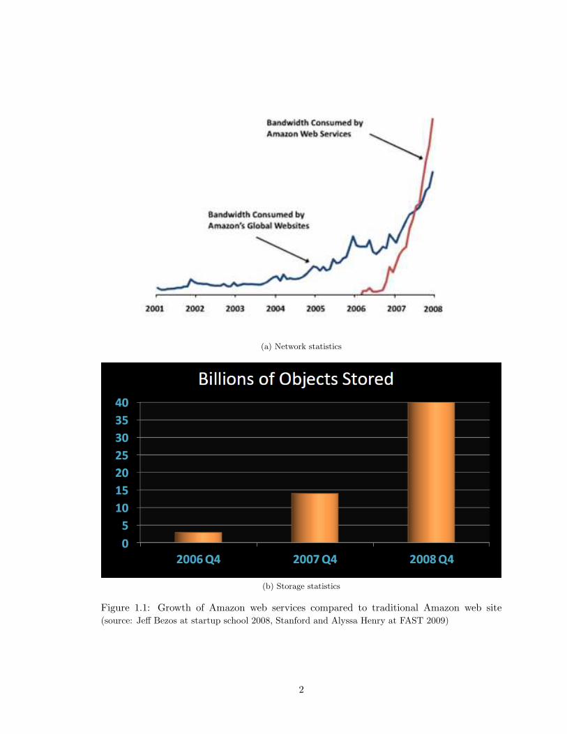
1.1 Growth of Amazon web services compared to traditional Amazon web site
(source: Jeff Bezos at startup school 2008, Stanford and Alyssa Henry at FAST 2009) 2
1.2 Distribution of CPU utilization in measurement analysis of PC usage data
at MSR India . . . . . . . . . . . . . . . . . . . . . . . . . . . . . . . . . . . 3
1.3 An example of data center server consumption . . . . . . . . . . . . . . . . 5
1.4 Resource usage in a production SAP application server for a one-day period. 7
2.1 Feedback loops in AutoControl . . . . . . . . . . . . . . . . . . . . . . . . . 24
3.1 A testbed of two virtualized servers hosting two multi-tier applications . . . 29
3.2 An input-output model for a multi-tier application . . . . . . . . . . . . . . 31
3.3 Input-output relationship in a two-tier RUBiS application for [500, 700, 900,
1100] clients . . . . . . . . . . . . . . . . . . . . . . . . . . . . . . . . . . . . 31
3.4 Loss ratio and response time ratio for two RUBiS applications in the WS-DU
scenario . . . . . . . . . . . . . . . . . . . . . . . . . . . . . . . . . . . . . . 37
3.5 Response time ratio for two TPC-W applications in the WU-DS scenario . 40
3.6 A two-layered controller architecture . . . . . . . . . . . . . . . . . . . . . . 42
3.7 Adaptive utilization controller . . . . . . . . . . . . . . . . . . . . . . . . . . 43
3.8 Utilization controller results in the WU-DU case . . . . . . . . . . . . . . . 46
3.9 Loss ratio experiment results . . . . . . . . . . . . . . . . . . . . . . . . . . 48
3.10 RT ratio experiment results . . . . . . . . . . . . . . . . . . . . . . . . . . . 49
3.11 RT ratio experiments - time-varying workload, with controller . . . . . . . . 52
ix

3.12 RT ratio experiments - time-varying workload, without controller . . . . . . 53
3.13 Database heavy load - with controller . . . . . . . . . . . . . . . . . . . . . 54
3.14 Database heavy load - without controller . . . . . . . . . . . . . . . . . . . . 55
4.1 Physical organization: Each node hosts multiple applications running on
VMs. Applications can span multiple nodes . . . . . . . . . . . . . . . . . . 59
4.2 Logical controller organization: Each application has one application
controller. Each node has one node controller that arbitrates the requests
from multiple application controllers . . . . . . . . . . . . . . . . . . . . . . 60
4.3 AppController’s internal structure . . . . . . . . . . . . . . . . . . . . . . . 63
4.4 Average performance overhead . . . . . . . . . . . . . . . . . . . . . . . . . 69
4.5 SLOC of major code components . . . . . . . . . . . . . . . . . . . . . . . . 69
4.6 A virtualized node in the testbed . . . . . . . . . . . . . . . . . . . . . . . . 70
4.7 Experimental setup . . . . . . . . . . . . . . . . . . . . . . . . . . . . . . . . 70
4.8 Application throughput with bottlenecks in CPU or disk I/O and across
multiple nodes . . . . . . . . . . . . . . . . . . . . . . . . . . . . . . . . . . 74
4.9 Resource allocations to different applications or application tiers on different
nodes . . . . . . . . . . . . . . . . . . . . . . . . . . . . . . . . . . . . . . . 75
4.10 Internal workings of the AppController - model estimator performance . . . 78
4.11 Performance comparison between AutoControl and work-conserving mode,
with different priority weights for TPC-W (w = 2) and smedia3 (w = 1). . . 81
4.12 Performance results for TPC-W and smedia3 with stability factor q = 1, 2, 10 81
4.13 Performance comparison of AutoControl, work-conserving mode and static al-
location mode, while running RUBiS, smedia1 and smedia2 with production-
trace-driven workloads. . . . . . . . . . . . . . . . . . . . . . . . . . . . . . . 82
4.14 SLO violations in 64 applications using work-conserving mode and AutoControl 85
4.15 Behavior of Smedia Application During Migration . . . . . . . . . . . . . . 86
5.1 Storage system consists of a shared disk array with independent proportional
share I/O scheduler running at each port. . . . . . . . . . . . . . . . . . . . 90
5.2 Architecture of the Storage QoS controller. . . . . . . . . . . . . . . . . . . 91
x
5.3 Performance of a changing workload with throughput targets. The control
interval is 2 seconds. . . . . . . . . . . . . . . . . . . . . . . . . . . . . . . . 96
5.4 Workloads with different target metrics. The light workload has a through-
put target of 20 MB/sec and the heavy workload has a latency target of
10ms. . . . . . . . . . . . . . . . . . . . . . . . . . . . . . . . . . . . . . . . 97
5.5 Effects of workload priorities. . . . . . . . . . . . . . . . . . . . . . . . . . . 98
6.1 Analysis of PC usage data at MSR India . . . . . . . . . . . . . . . . . . . . 108
6.2 LiteGreen architecture: Desktops are in active (switched on) or idle
(sleep) state. Server hosts idle desktops running in VMs . . . . . . . . . . . 110
6.3 Desktop states . . . . . . . . . . . . . . . . . . . . . . . . . . . . . . . . . . 111
6.4 Migration timelines . . . . . . . . . . . . . . . . . . . . . . . . . . . . . . . . 120
6.5 Distribution of desktop sleep durations . . . . . . . . . . . . . . . . . . . . . 123
6.6 Number of migrations . . . . . . . . . . . . . . . . . . . . . . . . . . . . . . 123
6.7 Xen experiments . . . . . . . . . . . . . . . . . . . . . . . . . . . . . . . . . 124
6.8 Energy savings from existing power management and LiteGreen’s default and
conservative policies . . . . . . . . . . . . . . . . . . . . . . . . . . . . . . . 127
6.9 Resource utilization during idle desktop consolidation . . . . . . . . . . . . 128
6.10 CPU utilization of selected users . . . . . . . . . . . . . . . . . . . . . . . . 131
7.1 An example of data center server consumption . . . . . . . . . . . . . . . . 134
7.2 System architecture . . . . . . . . . . . . . . . . . . . . . . . . . . . . . . . 136
7.3 Various configurations for consolidation . . . . . . . . . . . . . . . . . . . . 140
7.4 Single-node - application performance . . . . . . . . . . . . . . . . . . . . . 142
7.5 Single-node analysis results . . . . . . . . . . . . . . . . . . . . . . . . . . . 144
7.6 Two-node analysis results . . . . . . . . . . . . . . . . . . . . . . . . . . . . 146
7.7 Single-node vs. two-node - Xen Dom0 CPU consumption . . . . . . . . . . 147
7.8 Two-node - Oprofile analysis . . . . . . . . . . . . . . . . . . . . . . . . . . 148
7.9 Single-node vs. two-node - Oprofile analysis . . . . . . . . . . . . . . . . . . 148
7.10 two-node multiple instances - average response time . . . . . . . . . . . . . 152
xi
7.11 Comparison of all configurations (800 threads) . . . . . . . . . . . . . . . . 152
7.12 two-node multiple instances - Xen Dom0 CPU consumption . . . . . . . . . 152
7.13 two-node two instances - Oprofile analysis for Xen and OpenVZ . . . . . . . 153
7.14 Single instance vs. two instances - Oprofile analysis for Xen . . . . . . . . . 153
7.15 Single instance vs. and two instances - Oprofile analysis for OpenVZ . . . . 154
8.1 Combined metrics, thrref = 25, rtref = 10, α = 1, β = 1, thr = 0 − 50,
rt = 0− 15 . . . . . . . . . . . . . . . . . . . . . . . . . . . . . . . . . . . . 165
xii

LIST OF TABLES
TABLE
3.1 Four scenarios for two multi-tier applications . . . . . . . . . . . . . . . . . 38
4.1 Notation . . . . . . . . . . . . . . . . . . . . . . . . . . . . . . . . . . . . . . 62
4.2 Percentage of encrypted streams in each smedia application in different time
intervals . . . . . . . . . . . . . . . . . . . . . . . . . . . . . . . . . . . . . . 76
4.3 Predictive accuracy of linear models (in percentage) . . . . . . . . . . . . . 79
6.1 Statistics of PC usage data at MSR India . . . . . . . . . . . . . . . . . . . 107
6.2 Testbed details . . . . . . . . . . . . . . . . . . . . . . . . . . . . . . . . . . 119
6.3 Timing of individual steps in migration . . . . . . . . . . . . . . . . . . . . 121
6.4 Power measurements . . . . . . . . . . . . . . . . . . . . . . . . . . . . . . . 121
7.1 Base vs OpenVZ - % of L2 cache misses . . . . . . . . . . . . . . . . . . . . 145
7.2 Xen Web tier - % of L2 cache misses . . . . . . . . . . . . . . . . . . . . . . 145
7.3 Xen kernel - % of retired instructions . . . . . . . . . . . . . . . . . . . . . . 145
7.4 Base vs. OpenVZ - % cache misses/instruction for binaries . . . . . . . . . 146
7.5 Single-node vs. two-node - base system % of L2 cache misses . . . . . . . . 149
7.6 Single-node vs. two-node - OpenVZ % of L2 cache misses . . . . . . . . . . 149
7.7 Single-node vs. two-node - Xen Web tier % of L2 cache misses . . . . . . . 149
7.8 Single-node vs. two-node - Xen Web tier % of L2 cache misses/instruction 150
7.9 Web tier % L2 cache misses/instruction for binaries in Xen . . . . . . . . . 155
7.10 Web tier % of L2 cache misses in Xen kernel . . . . . . . . . . . . . . . . . . 156
7.11 Web tier % L2 cache misses/instruction for binaries and symbols in OpenVZ 156
xiii
ABSTRACT
Automated Management of Virtualized Data Centers
by
Pradeep Padala
Chair: Kang Geun Shin
Virtualized data centers enable sharing of resources among hosted applications. How-
ever, it is difficult to manage these data centers because of ever-changing application re-
quirements. This thesis presents a collection of tools called AutoControl and LiteGreen,
that automatically adapt to dynamic changes to achieve various SLOs (service level objec-
tives) while maintaining high resource utilization, high application performance and low
power consumption.
AutoControl resource manager is based on novel control theory and optimization tech-
niques. The central idea of this work is to apply control theory to solve resource allocation
in virtualized data centers while achieving applicaiton goals. Applying control theory to
computer systems, where first-principle models are not available, is a challenging task, and is
made difficult by the dynamics seen in real systems including changing workloads, multi-tier
dependencies, and resource bottleneck shifts.
To overcome the lack of first principle models, we build black-box models that not only
capture the relationship between application performance and resource allocations, but also
incorporate the dynamics of the system using an online adaptive model.
The next challenge is to design a controller that uses the online model to compute
optimal allocations to achieve applicaiton goals. We are faced with two conflicting goals:
quick response and stability. Our solution is an adaptive multi-input, multi-output (MIMO)
controller that uses a simplified Linear Quadratic Regulator (LQR) formulation. The LQR
xiv
formulation treats the control as an optimization problem and balances the tradeoff between
quick response and stability to find the right set of resource allocations to meet application
goals.
We also look at the idea of leveraging server consolidation to save desktop energy. Due
to the lack of energy proportionality in desktop systems, a great amount of energy is wasted
even when the system is idle. We design and implement a novel power manager called Lite-
Green to save desktop energy by virtualizing the users desktop computing environment as
a virtual machine (VM) and then migrating it between the user’s physical desktop ma-
chine and a VM server, depending on whether the desktop computing environment is being
actively used or is idle. A savings algorithm based on statistical inferences made from a
collection of traces is used to consolidate desktops on a remote server to save energy.
AutoControl and LiteGreen are built using Xen and Hyper-V virtualization technologies
and various experimental testbeds including a testbed on Emulab are built to evaluate
different aspects of AutoControl and LiteGreen.
xv
CHAPTER 1
Introduction
1.1 The Rise of Data Centers
There is a tremendous growth of data centers fueled by increasing demand for large-scale
processing. The growth is fueled by many factors including:
• Explosion of data in the cloud. Social networking site Facebook has 120 million users
with an average of 3% weekly growth since January 2007. E-mail services like Gmail
allows us to store every e-mail we ever sent or received.
• Growth of computing in the cloud. Services like Amazon EC2 [1] offer computing
power that can be dynamically allocated. Figure 1.1a shows the increase in network
bandwidth in Amazon web services. Figure 1.1b shows the explosion in S3 [42] storage
data.
• Increased demand for electronic transactions like on-line banking and trading.
• Growth of instant communication on the Internet. Twitter, a popular messaging site,
has grown from 300,000 users to 800,000 users in a matter of one year. Twitter servers
handle thousands of Tweets (instant messages) per second.
Today’s data centers hosting these applications often are designed with a silo-oriented
architecture in mind: each application has its own dedicated servers, storage and network
infrastructure, and a software stack tailored for the application that controls these resources
1
(a) Network statistics
(b) Storage statistics
Figure 1.1: Growth of Amazon web services compared to traditional Amazon web site(source: Jeff Bezos at startup school 2008, Stanford and Alyssa Henry at FAST 2009)
2
0
10
20
30
40
50
60
70
80
90
100
0 10 20 30 40 50 60 70 80 90 100
CD
F
CPU utilization
CPU with UICPU only
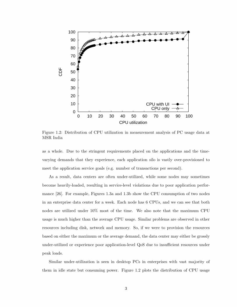
Figure 1.2: Distribution of CPU utilization in measurement analysis of PC usage data atMSR India
as a whole. Due to the stringent requirements placed on the applications and the time-
varying demands that they experience, each application silo is vastly over-provisioned to
meet the application service goals (e.g. number of transactions per second).
As a result, data centers are often under-utilized, while some nodes may sometimes
become heavily-loaded, resulting in service-level violations due to poor application perfor-
mance [26]. For example, Figures 1.3a and 1.3b show the CPU consumption of two nodes
in an enterprise data center for a week. Each node has 6 CPUs, and we can see that both
nodes are utilized under 10% most of the time. We also note that the maximum CPU
usage is much higher than the average CPU usage. Similar problems are observed in other
resources including disk, network and memory. So, if we were to provision the resources
based on either the maximum or the average demand, the data center may either be grossly
under-utilized or experience poor application-level QoS due to insufficient resources under
peak loads.
Similar under-utilization is seen in desktop PCs in enterprises with vast majority of
them in idle state but consuming power. Figure 1.2 plots the distribution of CPU usage
3
and UI activity, binned into 1-minute buckets and aggregated across all of the PCs in a
measurement study (more details in Chapter 6). To allow plotting both CPU usage and UI
activity in the same graph, we adopt the convention of treating the presence of UI activity
in a bucket as 100% CPU usage. The “CPU only” curve in the figure shows that CPU
usage is low, remaining under 10% for 90% of the time. The “CPU + UI” curve shows that
UI activity is present, on average, only in 10% of the 1-minute buckets, or about 2.4 hours
in a day.
Vast over-provisioning also causes high power consumption in the data centers. The
estimated amount of power consumption by data centers during 2006 in the US is 61 billion
kilowatt-hours (kWh) [24], which is about 1.5% of total US consumption of electricity. The
report [24] also noted that the energy usage of data centers in 2006 is estimated to be more
than double the energy consumed in 2000. Similar reports have also estimated that the
energy usage of desktops has skyrocketed. A recent study [74] estimates that PCs and their
monitors consume about 100 TWh/year, constituting 3% of the annual electricity consumed
in the U.S. Of this, 65 TWh/year is consumed by PCs in enterprises, which constitutes 5%
of the commercial building electricity consumption.
Virtualization is causing a disruptive change in enterprise data centers and giving rise to
a new paradigm: shared virtualized infrastructure. In this new paradigm, multiple enterprise
applications share dynamically allocated resources. These applications are also consolidated
to reduce infrastructure, operating, management, and power costs, while simultaneously
increasing resource utilization. Revisiting the previous scenario of two application servers,
Figure 1.3c shows the sum of the CPU consumptions from both nodes. It is evident that
the combined application demand is well within the capacity of one node at any particular
time. If we can dynamically allocate the server capacity to these two applications as their
demands change, we can easily consolidate these two nodes into one server.
1.2 Research Challenges
Unfortunately, the complex nature of enterprise desktop and server applications pose
further challenges for this new paradigm of shared data centers. Data center administrators
4

0 500 1000 1500 2000
0.5
1
1.5
2
2.5
3
Sample point(every 5 minutes)
CPU
cons
umpt
ion(
# of
CPU
s)
(a) CPU consumption of node 1
0 500 1000 1500 2000
0.5
1
1.5
2
Sample point(every 5 minutes)
CPU
cons
umpt
ion(
# of
CPU
s)
(b) CPU consumption of node 2
0 500 1000 1500 2000
1
2
3
4
Sample point (every 5 minutes)
CPU
cons
umpt
ion
(# o
f CPU
s)
(c) Sum of CPU consumptions from both nodes
Figure 1.3: An example of data center server consumption
are faced with growing challenges to meet service level objectives (SLOs) in the presence of
dynamic resource sharing and unpredictable interactions across many applications. These
challenges include:
• Complex SLOs: It is non-trivial to convert individual application SLOs to correspond-
ing resource shares in the shared virtualized platform. For example, determining the
5

amount of CPU and the disk shares required to achieve a specified number of financial
transactions per unit time is difficult.
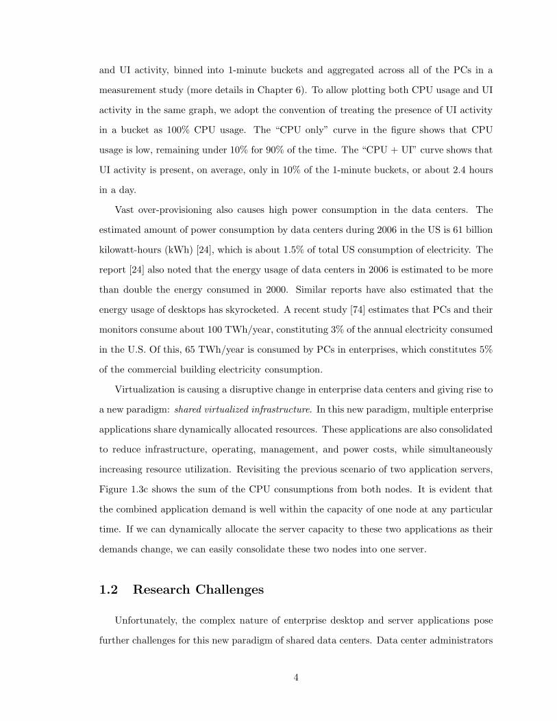
• Changing resource requirements over time: The intensity and the mix of enterprise ap-
plication workloads change over time. As a result, the demand for individual resource
types changes over the lifetime of the application. For example, Figure 1.4 shows
the CPU and disk utilization of an SAP application for a day. The utilization for
both resources varies over time considerably, and the peaks of the two resource types
occurred at different times of the day. This implies that static resource allocation
can meet application SLOs only when the resources are allocated for peak demands,
wasting a great deal of resources.
• Distributed resource allocation: Multi-tier applications spanning across multiple nodes
require resource allocations across all tiers to be at appropriate levels to meet end-to-
end application SLOs.
• Resource dependencies: Application-level performance often depends on the applica-
tion’s ability to simultaneously access multiple system-level resources.
• Complex power consumption: Consolidation of machines to reduce power consump-
tion is complicated by the fact that desktops have complex power usage behavior.
Many desktop applications have bursty resource demand, making a bad consolidation
decision affect application performance.
Researchers have studied capacity planning for such an environment by using historical
resource utilization traces to predict the application resource requirements in the future
and to place compatible sets of applications onto the shared nodes [82]. Such an approach
aims to ensure that each node has enough capacity to meet the aggregate demand of all
the applications, while minimizing the number of active nodes. However, past demands
are not always accurate predictors of future demands, especially for Web-based, interactive
applications. Furthermore, in a virtualized infrastructure, the performance of a given ap-
plication depends on other applications sharing resources, making it difficult to predict its
behavior using pre-consolidation traces. Other researchers have considered use of live VM
6
0
20
40
60
80
100
0 48 96 144 192 240 288
Reso
urc
e u
tiliz
atio
n (
%)
Time interval (every 5 mins)
CPU utilDisk util
Figure 1.4: Resource usage in a production SAP application server for a one-day period.
migration to alleviate overload conditions that occur at runtime [39]. However, the CPU
and network overheads of VM migration may further degrade application performance on
the already-congested node, and hence, VM migration is mainly effective for sustained,
rather than transient, overload.
To overcome the difficulties, in this thesis, we develop various tools for managing re-
sources and energy consumption as follows:
• AutoControl - resource manager: AutoControl is a feedback-based resource al-
location system that manages dynamic resource sharing within the virtualized nodes
and that complements the capacity planning and workload migration schemes others
have proposed to achieve application-level SLOs on shared virtualized infrastructure.
• LiteGreen - power manager: LiteGreen is an automated system that consolidates
idle desktops onto a central server to reduce the energy consumption of desktops as a
whole. LiteGreen uses virtual machine migration to move idle desktops into a central
server. The desktop VM is moved back when the user comes back seamlessly and a
remote desktop client is used to mask the effect of migration.
7

1.3 Research Goals
The main theme of this research is: Automation. The goal of this work is to develop
automated mechanisms to meet application goals in a virtualized data center in changing
workload conditions.
1.3.1 AutoControl
We set the following goals in designing AutoControl :
Performance assurance: If all applications can meet their performance targets, Auto-
Control should allocate resources properly to achieve them. If they cannot be met,
AutoControl should provide service differentiation according to application priorities.
Automation: While performance targets and certain parameters within AutoControl may
be set manually, all allocation decisions should be made automatically without human
intervention.
Adaptation: The controller should adapt to variations in workloads or system conditions.
Scalability: The controller architecture should be distributed so that it can handle many
applications and nodes, and also limit the number of variables each controller deals
with.
1.3.2 LiteGreen
The following goals are set in designing LiteGreen:
Energy conservation: LiteGreen should try to conserve as much energy as possible, while
maintaining acceptable desktop application performance.
Automation: The decisions for consolidation of desktop applications should be done au-
tomatically.
Adaptation: The controller should adapt to variations in desktop workloads.
Scalability: The LiteGreen should be scalable to many desktops.
8
1.4 Research Contributions
As discussed in the previous sections, there are many challenges in managing complex
shared virtualized infrastructure. The AutoControl tools, we have developed, make the
management of these virtualized data centers easy.
More specifically, we make the following contributions.
1.4.1 Utilization-based CPU Resource Controller
In our earlier attempts to apply control theory, we have developed a two-layered con-
troller that accounts for the dependencies and interactions among multiple tiers in an appli-
cation stack when making resource allocation decisions. The controller is designed to adap-
tively adjust to varying workloads so that high resource utilization and high application-level
QoS (Quality of Service) can be achieved. Our design employs a utilization controller that
controls the resource allocation for a single application tier and an arbiter controller that
controls the resource allocations across multiple application tiers and multiple application
stacks sharing the same infrastructure.
This contribution is unique in providing a valuable insight into applying control theory
to a complex virtualized infrastructure. We have succeeded in applying control theory in
this simplified case, but there is more to be achieved, before we can claim that we have
built a completely automated management platform. This work is published in Eurosys
2007 and Chapter 3 in part, is a reprint of the published paper.
1.4.2 Multi-resource Controller
To address the deficiencies of CPU-only controller, we build a MIMO modeler and
controller that can control multiple resources. More specifically, our contributions are two-
fold.
1. Dynamic black-box modeler : We design an online model estimator to dynamically
determine and capture the relationship between application-level performance and the
allocation of individual resource shares. Our adaptive modeling approach captures the
complex behavior of enterprise applications including time-varying resource demands,
9

resource demands from distributed application tiers, and shifting demands across
multiple resource types.
2. Multi-input, multi-output controller : We design a two-layer, multi-input, multi-output
(MIMO) controller to automatically allocate multiple types of resources to enterprise
applications to achieve their SLOs. The first layer consists of a set of application
controllers that automatically determine the amount of resources necessary to achieve
individual application SLOs, using the estimated models and a feedback-based ap-
proach. The second layer is comprised of a set of node controllers that detect resource
bottlenecks on the shared nodes and properly allocate multiple types of resources to
individual applications. Under overload, the node controllers provide service differen-
tiation according to the priorities of individual applications.
This work is published in Eurosys 2009, and Chapter 4 in part, is a reprint of the
published paper.
1.4.3 Multi-port Storage Controller
We extend our multi-resource controller to solve a special case of controlling access to
multiple ports in a large-scale storage system to meet competing application goals.
Applications running on the shared storage present very different storage loads and
have different performance requirements. When the requirements of all applications cannot
be met, the choice of which application requirements to meet and which ones to abandon
may depend upon the priority of the individual applications. For example, meeting the I/O
response time requirement of an interactive system may take precedence over the throughput
requirement of a backup system. A data center operator needs the flexibility to set the
performance metrics and priority levels for the applications, and to adjust them as necessary.
The proposed solutions to this problem in the literature include using proportional share
I/O schedulers (e.g., SFQ [55]) and admission control (I/O throttling) using feedback con-
trollers (e.g., Triage [60]). Proportional share schedulers alone cannot provide application
performance differentiation for several reasons: First, the application performance depends
on the proportional share settings and the workload characteristics in a complex, non-linear,
10

time-dependent manner, and it is difficult for an administrator to determine in advance the
share to assign to each application, and how/when to change it. Second, applications have
several kinds of performance targets, such as response time and bandwidth requirements,
not just throughput. Finally, in overload situations, when the system is unable to meet
all of the application QoS requirements, prioritization is necessary to enable important
applications to meet their performance requirements.
We combine an optimization-based feedback controller with an underlying I/O sched-
uler. Our controller accepts performance metrics and targets from multiple applications,
monitors the performance of each application, and periodically adjusts the IO resources
given to the applications at the disk array to make sure that each application meets its per-
formance goal. The performance metrics for the applications can be different: the controller
normalizes the application metrics so that the performance received by different applica-
tions can be compared and traded off. Our controller continually models the performance
of each application relative to the resources it receives, and uses this model to determine
the appropriate resource allocation for the application. If the resources available are inade-
quate to provide all the applications with their desired performance, a Linear Programming
optimizer is used to compute a resource allocation that will degrade each application’s
performance in inverse proportion to its priority.
This work is published in International Workshop on Feedback Control Implementation
and Design in Computing Systems and Networks (FEBID) 2009, and Chapter 4 in part, is
a reprint of the published paper.
1.4.4 Idle Desktop Consolidation to Conserve Energy
While the previous work focused on consolidation of server workloads, we have also
looked at consolidating idle desktops onto servers to save energy. It is well-known that
desktops running in virtual machines can be consolidated onto servers, but it is unclear
how to do this while maintaining good user experience and low energy usage. If we keep
all desktops on the server and use thin clients to connect to them, energy usage is low, but
performance may suffer because of resource contention. Users also lose the ability to control
many aspects of their desktop environment (e.g., for playing games). On the other hand,
11
leaving all desktops on all the time gives high performance, and great user experience, but
loses on energy.
We present LiteGreen, a system to save desktop energy by employing a novel approach
to avoiding user disruption as well as the complexity of application-specific customization.
The basic idea of LiteGreen is to virtualize the user’s desktop computing environment as a
virtual machine (VM) and then migrate it between the user’s physical desktop machine and
a server hosting VMs, depending on whether the desktop computing environment is being
actively used or is idle. When the desktop becomes idle, say when the user steps away for
several minutes (e.g., for a coffee break), the desktop VM is migrated away to the VM server
and the physical desktop machine is put to sleep. When the desktop becomes active again
(e.g., when the user returns), the desktop VM is migrated back to the physical desktop
machine. Thus, even when it has been migrated to the VM server, the user’s desktop
environment remains alive (i.e., it is “always on”), so ongoing network connections and
other activity (e.g., background downloads) are not disturbed, regardless of the application
involved.
The “always on” feature of LiteGreen allows energy savings whenever the opportunity
arises, without having to worry about disrupting the user. Besides long idle periods (e.g.,
nights and weekends), energy can also be saved by putting the physical desktop computer
to sleep even during short idle periods, such as when a user goes to a meeting or steps out
for coffee.
More specifically, the main contributions of LiteGreen are as follows.
1. A novel system that leverages virtualization to consolidate idle desktops on a VM
server, thereby saving energy while avoiding user disruption.
2. Automated mechanisms to drive the migration of the desktop computing environment
between the physical desktop machines and the VM server.
3. A prototype implementation and the evaluation of LiteGreen through a small-scale
deployment.
4. Trace-driven analysis based on an aggregate of over 65,000 hours of desktop resource
12

usage data gathered from 120 desktops, demonstrating total energy savings of 72-86%.
1.4.5 Performance Evaluation of Server Consolidation
We have seen that server consolidation is not a trivial task, and we require many tech-
nologies including capacity planning, virtual machine migration, slicing and automated
resource allocation to achieve the best possible results. However, there is another aspect
of server consolidation that is often glossed over: virtualization technology. The explosive
growth of virtualization has produced many virtualization technologies including VMware
ESX [11], Xen [30], OpenVZ [6], and many more.
In this thesis, we try to answer a key research question: Which virtualization technology
works best in server consolidation and why?. We compare Xen (hypervisor-based technol-
ogy) and OpenVZ (OS container-based technology), and conclude that OpenVZ performs
better than Xen, but Xen provide more isolation.
1.5 Organization of the Thesis
The organization of the thesis closely follows the contributions mentioned above. We
first provide the background and related work in Chapter 2. Our first experience with
using control theory to build a CPU controller that allocates CPU resources to competing
multi-tier applications is described in Chapter 3. Design, implementation and evaluation
of a fully automated multi-resource controller is provided in Chapter 4. The special case
of applying multi-resource controller to multi-port large-scale storage system is presented
in Chapter 5. Consolidation of desktops for saving energy is described in Chapter 6. The
virtualization technologies Xen and OpenVZ are evaluated in Chapter 7 to get insight into
different aspects of the two technologies for server consolidation. The thesis is concluded
with avenues for future work in Chapter 8.
13
CHAPTER 2
Background and Related Work
In this chapter, we provide a broad overview of the background required to understand
the techniques described in the thesis. References to more detailed information are provided
for interested readers.
2.1 Virtualization
Virtualization refers to many different concepts in computer science [100], and is often
used to describe many types of abstractions. In this work, we are primarily concerned with
Platform Virtualization, which separates an operating system from the underlying hardware
resources. Virtual Machine (VM) refers to the abstracted machine that gives the illusion
of a “real machine”.
The earliest experiments with virtualization date back to 1960s, when IBM built VM/370
[40, 68] and operating system that gives the illusion of multiple independent machines.
VM/370 is built for System/370 mainframe computers built by IBM, and the virtualization
features are used to maintain backward compatibility with the instruction set in System/360
mainframes (precursor to System/370 mainframes). Similar attempts were made to provide
virtual machines on DEC PDP-10 [45].
The popularity of mainframes has declined in later years, with much lower priced high-
end servers taking their roles. With the advent of multi-core computing and ever increasing
power of servers, virtualization has seen resurgence. Research system Disco [33] is one
of the first research efforts to bring the old virtual machine concepts to the front. In
14
Disco, Stanford university researchers have developed a virtual machine monitor (VMM)
that allows multiple operating systems to run giving the illusion of multiple machines.
The techniques described in Disco are commercialized later by VMware [83]. Countless
commercial virtualization techniques followed VMware.
2.2 Virtualization Requirements
How to build virtual machines on a specific hardware architecture? - This is one of the
questions that irked researchers in the 70s, and Goldberg and Popek [77] are the first ones to
identify the hardware requirements to build a virtual machine. They define two important
concepts: virtual machine and virtual machine monitor (VMM).
1. A virtual machine is taken to be an efficient, isolated duplicate of the real
machine.
2. As a piece of software a VMM has three essential characteristics. First, the
VMM provides an environment for programs which is essentially identical
with the original machine; second, programs run in this environment show
at worst only minor decreases in speed; and last, the VMM is in complete
control of system resources.
Goldberg and Popek also define the requirements of an instruction set architecture (ISA)
to be virtualizable.
For any conventional third-generation computer, a VMM may be constructed
if the set of sensitive instructions for that computer is a subset of the set of
privileged instructions.
Before, we understand their requirements, we need define a few terms. Third generation
computers refer to computers based on integrated circuits. Other terms are defined as
follows:
• Privileged instructions: Those that trap if the processor is in user mode and do
not trap if it is in system mode.
15
• Control sensitive instructions: Those that attempt to change the configuration
of resources in the system.
• Behavior sensitive instructions: Those whose behavior or result depends on the
configuration of resources (the content of the relocation register or the processor’s
mode).
This simply states that if sensitive instructions can be executed in user-mode without
the VMM’s knowledge, VMM may no longer have the full control of resources violating the
third VMM property described above.
Intel’s x86 architecture, the predominant ISA in current computers is famously non-
virtualizable [62]. However, dynamic recompilation can be used to dynamically modify
sensitive instructions to trap so that VMM can take appropriate action. These techniques
have been used in many virtualization technologies including QEMU [31] and Virtual box
[9].
Another approach called para-virtualization, pioneered by Xen [30] makes minimal mod-
ifications to operating systems hosted by the VMM, so that sensitive instructions can be
handled appropriately.
The advent of virtualization enabled processors by Intel and AMD called VT-x and
AMD-V respectively allow hardware-assisted virtualization [91] which does not require any
modifications to operating systems.
2.2.1 Operating System Level Virtualization
VMMs described above provide a virtual machine that gives the illusion of a real ma-
chine. This allows running of multiple operating systems on the same physical hardware.
In a single operating system, however, partition of resources can be done such that mul-
tiple partitions do not harm each other. In earlier UNIX systems, these partitions are
implemented using chroot environment, and the multiple environments are called jails.
Though jails had some isolation, it was easy for one jail to impact another jail.
More sophisticated mechanisms called resource containers [29] have tried to build more
isolation. Many similar container architectures followed including [81, 6, 85] and many
16
commercial implementations [10] are available as well.
The main benefits of operating system level virtualization is performance, while sacri-
ficing some isolation. A more detailed comparison of hypervisor based virtualization and
operating system level virtualization is in Chapter 7.
2.3 Virtualized Data Centers
Though virtualization was originally seen as a technique to provide backward compat-
ibility and isolation among competing environments, it has given rise to virtualized data
centers. We define a virtualized data center as a data center running the applications only
in virtual machines.
2.3.1 Benefits of Virtualized Data Centers
Why do we want to run applications in a data center in virtual machines? - There are
many benefits to running applications in virtual machines compared to running on physical
machines including
1. High Utilization: As we saw in Chapter 1, sharing resources allows better utilization
of overall data center resources.
2. Performance Isolation: The applications can be isolated by running them in dif-
ferent virtual machine. Different virtualization technologies differing levels of perfor-
mance isolation, but most of them offer safety, correctness and fault-tolerance isola-
tion. Though many virtualization technologies can be used for isolation, we choose
hypervisor-based virtualization. The reasoning for choosing this method is described
in Chapter 7.
Though physical machine can offer isolation by running multiple applications in dif-
ferent physical machines, such scenario would waste great amount of resources.
3. Low Management Costs: Virtual machines allow easy provisioning of resources
in a data center and virtual machine migration [39] allows easy movement of virtual
machines to save energy and for other purposes.
17

4. High Adaptability: The resources to virtual machines can be dynamically changed
allowing highly adaptive data centers. Major portion of this thesis is concerned with
creating a dynamic resource control system that can make automatic decisions for
high adaptability.
However, virtualization is not free, and causes overhead that may not be suitable for
some applications.
2.4 Server Consolidation
The main benefit of virtualized data centers comes from server consolidation, in which
multiple applications are consolidated onto a single physical machine. However, figuring
out the right way to consolidate still remains an unsolved research problem.
2.4.1 Capacity Planning
Traditionally consolidation is done through capacity planning. Researchers have stud-
ied capacity planning for such an environment by using historical resource utilization traces
to predict application resource requirements in the future and to place compatible sets
of applications onto shared nodes [82]. This approach aims to ensure that each node has
enough capacity to meet the aggregate demand of all the applications, while minimizing the
number of active nodes. However, past demands are not always accurate predictors of fu-
ture demands, especially for Web-based, interactive applications. Furthermore, in a shared
virtualized infrastructure, the performance of a given application depends on other appli-
cations sharing resources, making it difficult to predict its behavior using pre-consolidation
traces.
2.4.2 Virtual Machine Migration
Virtual machine migration involves migration of a running VM from one machine to
another machine where it can continue execution. Migration is made practical with tech-
niques that allow live migration [39], where the original VM continues to run while VM is
18
being migrated, and has a very low downtime.
Live migration allows movement of resources based on VM resource usage and many
strategies have been proposed for the allocation [101, 92].
2.4.3 Resource Allocation using Slicing
There are many ways to allocate resources in a single machine, in this work we primarily
focus on proportional sharing. Proportional sharing is often touted as the mechanism to
allocate resources in certain ratio (also called shares), as that allows operators to specify
the ratios to achieve certain quality of service for individual applications.
Proportional share schedulers allow reserving CPU capacity for applications [56, 72, 94].
While these can enforce the desired CPU shares, our controller also dynamically adjusts
these share values based on application-level QoS metrics. It is similar to the feedback
controller in [87] that allocates CPU to threads based on an estimate of each thread’s
progress, but our controller operates at a much higher layer based on end-to-end application
performance that spans multiple tiers in a given application.
In the past few years, there has been a great amount of research in improving schedul-
ing in virtualization mechanisms. Virtualization technologies including VMware [83] and
Xen [30], offer proportional share schedulers for CPU in the hypervisor layer that can be
used to set the allocation for a particular VM. However, these schedulers only provide
mechanisms for controlling resources. One also has to provide the right parameters to the
schedulers in order to achieve desired application-level goals.
For example, Xen’s CPU credit scheduler provides two knobs: cap and share. The cap
allows one to set a hard limit on the amount of CPU used by a VM. The share knob is
expected to be used for proportional sharing. However, in our practice we found out that
using caps as the single knob for enforcing proportions works better than trying to use both
knobs together.
Xen does not provide any native mechanisms for allocating storage resources to individ-
ual VMs. Prior work on controlling storage resources independent of CPU includes systems
that provide performance guarantees in storage systems [36, 47, 55, 65]. However, one has
to tune these tools to achieve application-level guarantees. Our work builds on top of oth-
19
ers work, where the authors developed an adaptive controller [59] to achieve performance
differentiation, and efficient adaptive proportional share scheduler [48] for storage systems.
Similar to storage, knobs for network resources are not yet fully developed in virtu-
alization environments. Our initial efforts in adding network resource control have failed,
because of inaccuracies in network actuators. Since Xen’s native network control is not fully
implemented, we tried to use Linux’s existing traffic controller (tc) to allocate network re-
sources to VMs. We found that the network bandwidth setting in (tc) is not enforced
correctly when heavy network workloads are run. However, the theory we developed in this
work is directly applicable to any number of resources.
The memory ballooning supported in VMware [93] provides a way of controlling the
memory required by a VM. However, the ballooning algorithm does not know about appli-
cation goals or multiple tiers, and only uses the memory pressure as seen by the operating
system. We have done preliminary work [54] in controlling CPU and memory together
with other researchers. In many consolidation scenarios, memory is the limiting factor in
achieving high consolidation.
2.4.4 Slicing and AutoControl
In this thesis, we do not intend to replace capacity planning or migration mechanisms,
but augment them by dynamic resource allocation that manages dynamic resource sharing
within the virtualized nodes.
We assume that the initial placement of applications onto nodes has been handled by a
separate capacity planning service. The same service can also perform admission control for
new applications and determine if existing nodes have enough idle capacity to accommodate
the projected demands of the applications [82]. We also assume that a workload migration
system [101] may re-balance workloads among nodes at a time scale of minutes or longer.
These problems are complementary to the problem solved by AutoControl. Our system
deals with runtime management of applications sharing virtualized nodes, and dynamically
adjusts resource allocations over short time scales (e.g., seconds) to meet the application
SLOs. When any resource on a shared node becomes a bottleneck due to unpredicted
spikes in some workloads, or because of complex interactions between co-hosted applica-
20
tions, AutoControl provides performance differentiation so that higher-priority applications
experience lower performance degradation.
2.4.5 Migration for Dealing with Bottlenecks
Naturally, the question arises about whether we can use migration as the sole mecha-
nism for re-balancing. AutoControl enables dynamic re-distribution of resources between
competing applications to meet their targets, so long as sufficient resources are available. If
a node is persistently overloaded, VM migration [39, 101] may be needed, but the overhead
of migration can cause additional SLO violations. We performed experiments to quantify
these violations. A detailed study showing this behavior is provided in Chapter 4.
2.4.6 Performance Evaluation of Server Consolidation
In this thesis, we evaluate the two virtualization technologies Xen and OpenVZ for server
consolidation. Our work was motivated by the need for understanding server consolidation
in different virtualization technologies.
A performance evaluation of Xen was provided in the first SOSP paper on Xen [30] that
measured its performance using SPEC CPU2000, OSDB, dbench and SPECWeb bench-
marks. The performance was compared to VMWare, Base Linux and User-mode Linux.
The results have been re-produced by a separate group of researchers [38]. In this thesis,
we extend this evaluation to include OpenVZ as another virtualization platform, and test
both Xen and OpenVZ under different scenarios including multiple VMs and multi-tiered
systems. We also take a deeper look into some of these scenarios using OProfile [7] to
provide some insight into the possible causes of the performance overhead observed.
Menon et al. [67] conducted a similar performance evaluation of the Xen environment
and found various overheads in the networking stack. The work provides an invaluable
performance analysis tool Xenoprof that allows detailed analysis of a Xen system. The
authors identified the specific kernel subsystems that were causing the overheads. We
perform a similar analysis at a macro level and apply it to different configurations specifically
in the context of server consolidation. We also investigate the differences between OpenVZ
21
and Xen specifically related to performance overheads.
Menon et al. [66] use the information gathered in the above work and investigate causes
of the network overhead in Xen. They propose three techniques for optimizing network
virtualization in Xen. We believe that our work can help develop similar optimizations that
help server consolidation in both OpenVZ and Xen.
Soltesz et al. [85] have developed Linux VServer, which is another implementation of
container-based virtualization technology on Linux. They have done a comparison study be-
tween VServer and Xen in terms of performance and isolation capabilities. In this thesis, we
conduct performance evaluation comparing OpenVZ and Xen when used for consolidating
multi-tiered applications, and provide detailed analysis of possible overheads.
Gupta et al. [49] have studied the performance isolation provided by Xen. In their work,
they develop a set of primitives to address the problem of proper accounting of work done
in device drivers by a particular domain. Similar to our work, they use XenMon [50] to
detect performance anomalies. Our work is orthogonal to theirs by providing insight into
using Xen vs. OpenVZ and different consolidation techniques.
Server consolidation using virtual containers brings new challenges and, we comprehen-
sively evaluate two representative virtualization technologies in a number of different server
consolidation scenarios. See Chapter 7 for the full evaluation.
2.5 Resource Control before Virtualization
Dynamic resource allocation in distributed systems has been studied extensively, but
the emphasis has been on allocating resources across multiple nodes rather than in time,
because of lack of good isolation mechanisms like virtualization. It was formulated as an
online optimization problem in [27] using periodic utilization measurements, and resource
allocation was implemented via request distribution. Resource provisioning for large clus-
ters hosting multiple services was modeled as a “bidding” process in order to save energy in
[37]. The active server set of each service was dynamically resized adapting to the offered
load. In [84], an integrated framework was proposed combining a cluster-level load balancer
and a node-level class-aware scheduler to achieve both overall system efficiency and indi-
22
vidual response time goals. However, these existing techniques are not directly applicable
to allocating resources to applications running in VMs. They also fall short of providing a
way of allocating resources to meet the end-to-end SLOs.
Our approach of achieving QoS in virtualized data centers differs from achieving QoS
for OS processes. Earlier work focused on processes often had to deal with the lack of
good isolation mechanisms, and more focus was spent on building the mechanisms like
proportional share scheduling. Earlier work on OS processes also did not look at allocation
of multiple resources to achieve end-to-end application QoS.
2.6 Admission Control
Traditional admission control to prevent computing systems from being overloaded has
focused mostly on web servers. A “gatekeeper” proxy developed in [44] accepts requests
based on both online measurements of service times and offline capacity estimation for web
sites with dynamic content. Control theory was applied in [57] for the design of a self-
tuning admission controller for 3-tier web sites. In [59], a self-tuning adaptive controller
was developed for admission control in storage systems based on online estimation of the
relationship between the admitted load and the achieved performance. These admission
control schemes are complementary to the our approach, because the former shapes the
resource demand into a server system, whereas the latter adjusts the supply of resources
for handling the demand.
2.7 A Primer on Applying Control Theory to Computer Sys-
tems
Control theory is a rich body of theoretical work that is used to control dynamic systems.
Though, this thesis is about building a system for automated management, a major part
of this thesis uses control theory to solve important problems. Applying control theory to
computer systems is still an evolving field. For a detailed study of applying control theory
to computing systems, see [53]. In this section, we provide a brief primer on how to apply
23
(a) Standard control feedback loop
(b) Simplified AutoControl feedback loop
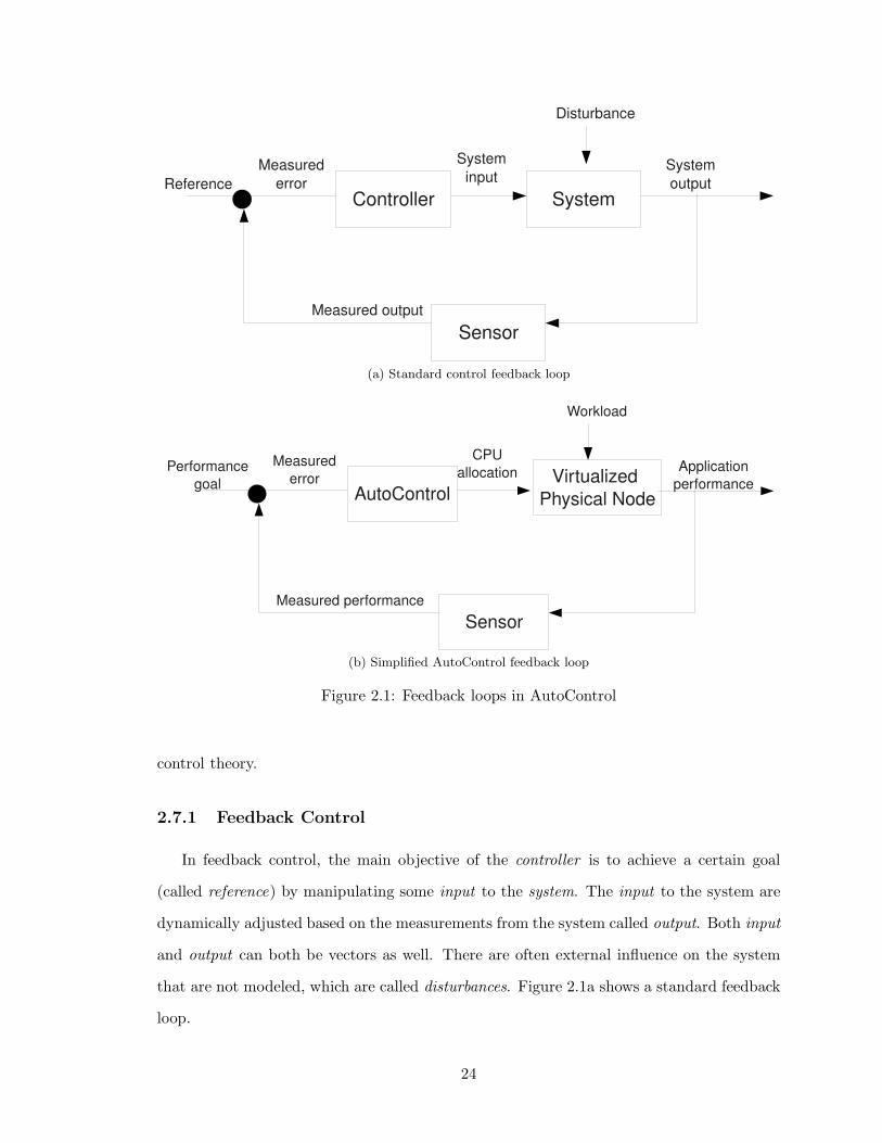
Figure 2.1: Feedback loops in AutoControl
control theory.
2.7.1 Feedback Control
In feedback control, the main objective of the controller is to achieve a certain goal
(called reference) by manipulating some input to the system. The input to the system are
dynamically adjusted based on the measurements from the system called output. Both input
and output can both be vectors as well. There are often external influence on the system
that are not modeled, which are called disturbances. Figure 2.1a shows a standard feedback
loop.
24
When applied to virtualized data centers, the system is a single physical node or multiple
physical nodes running virtual machines. The input to the system is the resource allocation
for the VMs. The output is the performance of application and the reference is the SLO for
the performance metric. We consider workload as the disturbance in this case. Figure 2.1b
shows the various elements in the AutoControl feedback loop. For simplicity, only CPU
resource is shown, and a single physical node is used as the system.
2.7.2 Modeling
The traditional way to designing controller in classical control theory is to first build
and analyze a model of the system, and then to develop a controller based on the model.
For traditional control systems, such models are often based on first principles. For
computer systems, although there is queueing theory that allows for analysis of aggregate
statistical measures of quantities such as utilization and latency, it may not be fine-grained
enough for run-time control over short time scales, and its assumption about the arrival
process or service time distribution may not be met by certain applications and systems.
Therefore, most prior work on applying control theory to computer systems employs an em-
pirical and “black box” approach to system modeling by varying the inputs in the operating
region and observing the corresponding outputs. We adopted this approach in our work.
2.7.3 Offline and Online Black Box Modeling
To build a black box model describing a computer system, we run the system in various
operating conditions, when we dynamically vary the inputs to the system and observe the
outputs. For example, a web server can be stressed by dynamically adjusting its resource
allocation, and observing the throughput and response time, where the number of serving
threads is being changed in each experiment. This is the approach used in build a CPU
controller in Chapter 3. After observing the system in many operating conditions, a model
can be developed based on the collected measurements often using regression techniques.
However, this offline modeling approach suffers from the problem of not being able to
adapt to changing workloads and conditions. It is impossible to completely model a system
25
prior to the production deployment, so an online adaptive approach is needed. In chapters
4 and 5, we build a dynamic system based on sophisticated adaptive modeling techniques.
2.7.4 Designing a Controller
In traditional control theory, the controller is often built by making use of standard
proportional (P), integral(I), derivative(D), PI, PID or other non-linear controllers [53].
There is a rich body of literature describing these controllers, and one can often use them
directly in certain systems.
However, for computer systems, often the models are not derived from first principles,
so black-box models with adaptive controllers are required. Adaptive control [28] again
contains a large body of research that allows changing of the control law based on dynamic
conditions. We refer the reader to [28] for a detailed study.
In this work, we have used an adaptive integral controller and adaptive multiple-input,
multiple-output optimal controllers, details of which are described in subsequent chapters.
2.7.5 Testing Controllers
In traditional control theory, controllers are theoretically analyzed for various proper-
ties including stability, optimality and robustness. The analysis often depends on model
construction and how the models are evaluated.
In this work, since we use black box models and adaptive control, it is often difficult
to directly apply theoretical analysis to test the controllers. We use a methodical systems
approach, where the controller is evaluated in various operating conditions. Along with the
classical control theory metrics, we also evaluate our system for scalability and performance.
2.8 Control Theory Based Related Work
In recent years, control theory has been applied to computer systems for resource man-
agement and performance control [52, 58]. Examples of its application include web server
performance guarantees [22], dynamic adjustment of the cache size for multiple request
classes [64], CPU and memory utilization control in web servers [43], adjustment of re-
26
source demands of virtual machines based on resource availability [103], and dynamic CPU
allocations for multi-tier applications [63, 76]. These concerned themselves with controlling
only a single resource (usually CPU), used mostly single-input single-output (SISO) con-
trollers (except in [43]), and required changes in the applications. In contrast, our MIMO
controller operates on multiple resources (CPU and storage) and uses the sensors and actua-
tors at the virtualization layer and external QoS sensors without requiring any modifications
to applications.
In [43], the authors apply MIMO control to adjust two configuration parameters within
Apache to regulate CPU and memory utilization of the Web server. They used fixed linear
models, which are obtained by offline system identification for modeling the system. Our
earlier attempts at fixed models for controlling CPU and disk resources have failed, and
therefore, we used an online adaptive model in this thesis. Our work also extends MIMO
control to controlling multiple resources and virtualization, which has more complex inter-
actions than controlling a single web server.
In [95], the authors build a cluster-level power controller that can distribute power
based on the application performance needs. The authors develop a MIMO controller for
achieveing the power distribution, which is similar to our approach.
27
CHAPTER 3
Utilization-based CPU Resource Controller
3.1 Introduction
In our first attempt to apply control theory to resource allocation in virtualized systems,
we have built an integral controller that allocates CPU resource based on QoS differentiation
metric. We address the problem of dynamically controlling resource allocations to individual
components of complex, multi-tier enterprise applications in a shared hosting environment.
We rely on control theory as the basis for modeling and designing such a feedback-driven
resource control system. We develop a two-layered controller architecture that accounts
for the dependencies and interactions among multiple tiers in an application stack when
making resource allocation decisions. The controller is designed to adaptively adjust to
varying workloads so that high resource utilization and high application-level QoS can be
achieved. Our design employs a utilization controller that controls the resource allocation for
a single application tier and an arbiter controller that controls the resource allocations across
multiple application tiers and multiple application stacks sharing the same infrastructure.
To test our controllers, we have built a testbed for a virtual data center using Xen
virtual machines (VMs)[30]. We encapsulate each tier of an application stack in a virtual
machine and attempt to control the resource allocation at the VM level. We experimented
with two multi-tier applications in our testbed: a two-tier implementation of RUBiS [25],
an online auction application, and a two-tier Java implementation of TPC-W [34], an on-
line ecommerce application. We ran experiments to test our controller under a variety of
28
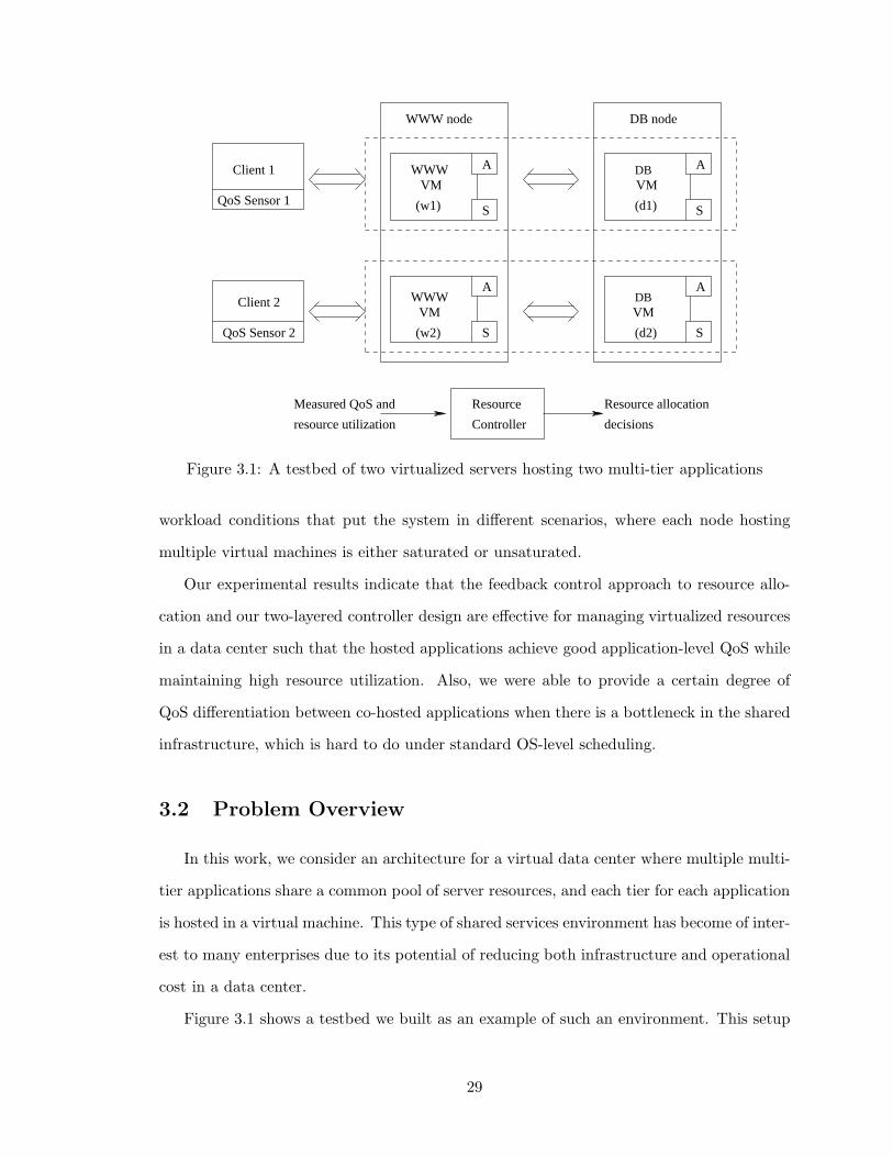
DB
DB
(w1)
S
A
Controller
Resource
resource utilization
Measured QoS and
Client 1
QoS Sensor 1
Client 2
QoS Sensor 2
WWW node DB node
(d1)
A
S
(d2)
Resource allocation
decisions
A
S
S
A
VM
VM
VMWWW
WWW VM
(w2)
Figure 3.1: A testbed of two virtualized servers hosting two multi-tier applications
workload conditions that put the system in different scenarios, where each node hosting
multiple virtual machines is either saturated or unsaturated.
Our experimental results indicate that the feedback control approach to resource allo-
cation and our two-layered controller design are effective for managing virtualized resources
in a data center such that the hosted applications achieve good application-level QoS while
maintaining high resource utilization. Also, we were able to provide a certain degree of
QoS differentiation between co-hosted applications when there is a bottleneck in the shared
infrastructure, which is hard to do under standard OS-level scheduling.
3.2 Problem Overview
In this work, we consider an architecture for a virtual data center where multiple multi-
tier applications share a common pool of server resources, and each tier for each application
is hosted in a virtual machine. This type of shared services environment has become of inter-
est to many enterprises due to its potential of reducing both infrastructure and operational
cost in a data center.
Figure 3.1 shows a testbed we built as an example of such an environment. This setup
29

forms a small but powerful system, which allows for testing our controller in various sce-
narios. To avoid confusion in terminology, we use “WWW VM” and “DB VM” to refer
to the two virtual machines that are used to host the web server and DB server software,
respectively. We use “WWW node” and “DB node” to refer to the two physical machines
that are used to host the web tier and the DB tier, respectively.
The high level goal of the resource controller is to guarantee application-level QoS as
much as possible while increasing resource utilization in a utility computing environment.
More specifically, our controller design has the following three main objectives:
• Guaranteed application-level QoS: When system resources are shared by multiple
multi-tier applications, it is desirable to maintain performance isolation between them
and to ensure that each application can achieve its QoS goals. In this work, this
is realized by dynamically allocating virtualized resources to each virtual machine
hosting an application component and always providing a safety margin below 100%
utilization if possible, which generally leads to high throughput and low response time
in the application.
• High resource utilization: It is also desirable to increase overall utilization of the
shared resources so that more applications can be hosted. One way to achieve this is
to maintain a high enough utilization in individual virtual machines such that there is
more capacity for hosting other applications. There is a fundamental trade-off between
this goal and the previous goal. It is up to the data center operators to choose an
appropriate utilization level to balance these two objectives.
• QoS differentiation during resource contention: Whenever a bottleneck is de-
tected in the shared resources, the controller needs to provide a certain level of QoS
differentiation that gives higher priority to more critical applications. For example,
one can aim to maintain a certain ratio of response times when the system is over-
loaded based on service level agreements of the respective applications.
30

WWW entitlement
DB entitlement
d
Workload
wDB utilization
drApplication
Multi−tierw(u )
(u )
(d)
r( )
( )
(y)QoS metrics
WWW utilization
Figure 3.2: An input-output model for a multi-tier application
0
20
40
60
80
100
10 20 30 40 50 60 70 80
CP
U C
onsu
mpt
ion
(% C
PU
)
WWW entitlement (% CPU)
500 clients700 clients900 clients
1100 clientsWWW entitlement
(a) WWW CPU consumption
0
20
40
60
80
100
10 20 30 40 50 60 70 80
CP
U C
onsu
mpt
ion
(% C
PU
)
WWW entitlement (% CPU)
500 clients700 clients900 clients
1100 clientsDB entitlement
(b) DB CPU consumption
0
20
40
60
80
100
10 20 30 40 50 60 70 80
CP
U C
onsu
mpt
ion
(% C
PU
)
WWW entitlement (% CPU)
500 clients700 clients900 clients
1100 clientsdom0 entitlement
(c) dom0 CPU consumption
0
20
40
60
80
100
10 20 30 40 50 60 70 80
WW
W u
tiliz
atio
n
WWW entitlement (% CPU)
500 clients700 clients900 clients
1100 clients
(d) WWW VM utilization
60
80
100
120
140
160
180
200
220
10 20 30 40 50 60 70 80
Thr
ough
put (
reqs
/sec
)
WWW entitlement (% CPU)
Offered (500 clients)Real (500 clients)
Offered (700 clients)Real (700 clients)
Offered (900 clients)Real (900 clients)
Offered (1100 clients)Real (1100 clients)
(e) Throughput
0
1
2
3
4
5
6
7
10 20 30 40 50 60 70 80
Res
pons
e T
ime
(sec
s)
WWW entitlement (% CPU)
500 clients700 clients900 clients
1100 clients
(f) Response time
Figure 3.3: Input-output relationship in a two-tier RUBiS application for [500, 700, 900,1100] clients
31
3.3 System Modeling
In control theory, an object to be controlled is typically represented as an input-output
system, where the inputs are the control knobs and the outputs are the metrics being con-
trolled. Control theory mandates that a system model that characterizes the relationship
between the inputs and the outputs be specified and analyzed before a controller is de-
signed. For traditional control systems, such models are often based on first principles. For
computer systems, although there is queueing theory that allows for analysis of aggregate
statistical measures of quantities such as utilization and latency, it may not be fine-grained
enough for run-time control over short time scales, and its assumption about the arrival
process may not be met by certain applications and systems. Therefore, most prior work
on applying control theory to computer systems employs an empirical and “black box” ap-
proach to system modeling by varying the inputs in the operating region and observing the
corresponding outputs. We adopted this approach in our work.
A feedback control loop requires an actuator to implement the changes indicated by the
control knobs and a sensor to measure the value of the output variables. We use the CPU
scheduler of the virtual machine monitor (or hypervisor) that controls the virtual machines
as our actuator. The hypervisor we used provides an SEDF (Simple Earliest Deadline First)
scheduler that implements weighted fair sharing of the CPU capacity between multiple
virtual machines. The scheduler allocates each virtual machine a certain share of the CPU
cycles in a given fixed-length time interval. Since these shares can be changed at run time,
the scheduler serves as an actuator (A) in our control loop to effect allocation decisions made
by the controller. The SEDF scheduler can operate in two modes: capped and non-capped.
In the capped (or non-work-conserving) mode, a virtual machine cannot use more than its
share of the total CPU time in any interval, even if there are idle CPU cycles available.
In contrast, in the non-capped (or work-conserving) mode, a virtual machine can use extra
CPU time beyond its share if other virtual machines do not need it. We use the capped
mode in our implementation as it provides better performance isolation between the VMs
sharing the same physical server.
The hypervisor also provides a sensor (S) to measure how many of the allocated CPU cy-
32
cles are actually consumed by each virtual machine in a given period of time. This gives the
resource controller information on utilization levels of individual virtual machines. In addi-
tion, we modified the RUBiS client and the TPC-W client to generate various application-
level QoS metrics, including average response time and throughput in a given period.
Before describing our modeling approach, we first define some terminology. We use
“entitlement” (u) to refer to the CPU share (in percentage of total CPU capacity) allocated
to a virtual machine. We use “consumption” (v) to refer to the percentage of total CPU
capacity actually used by the virtual machine. The term “VM utilization” (r) is used to
refer to the ratio between consumption and entitlement, i.e., r = v/u. For example, if a
virtual machine is allocated 40% of the total CPU and only uses 20% of the total CPU
on average, then its CPU entitlement is 40%, the CPU consumption is 20%, and the VM
utilization is 20%/40% = 50%. Note that all of these terms are defined for a given time
interval.
Figure 3.2 illustrates an input-output representation of the system we are controlling, a
multi-tier application hosted in multiple virtual machines. The inputs to the system are the
resource entitlements for the WWW VM (uw) and the DB VM (ud). The outputs include
the utilizations of the WWW VM (rw) and the DB VM (rd), as well as the application-
level QoS metrics (y) such as response time and throughput. The incoming workload (d)
to the hosted application is viewed as a “disturbance” to the controlled system because it
is not directly under control while having an impact on the system outputs. Typically as
the workload varies, the input-output relationship changes accordingly, which increases the
difficulty in modeling as well as controller design.
In the remainder of this section, we first describe our experimental testbed. Then we
describe a set of system modeling experiments we performed to determine a model for the
dynamic behavior of our multi-tier application under various configurations. Our modeling
experiments consists of two parts. First, we model the dynamic behavior of a single instance
of our multi-tier application, and then we develop a model for the dynamic behavior of two
multi-tier applications sharing the same infrastructure.
33
3.3.1 Experimental Testbed
Our experimental testbed consists of five HP Proliant servers, two of which are used
to host two applications. Each application consists of two tiers, a web server tier and a
database server tier. Apache and MySQL are used as the web server and database server,
respectively, hosted inside individual virtual machines. Although the grouping of application
tiers on each physical server can be arbitrary in principle, we specifically chose the design
where one machine hosts two web servers and the other hosts two DB servers. This is a
natural choice for many consolidated data centers for potential savings in software licensing
costs.
We chose Xen as the virtualization technology and we use Xen-enabled 2.6 SMP Linux
kernel in a stock Fedora 4 distribution. Each of the server nodes has two processors, 4 GB of
RAM, one Gigabit Ethernet interface, and two local SCSI disks. These hardware resources
are shared between the virtual machines (or domains in Xen terminology) that host the
application components and the management virtual machine (which we will refer as dom0
as in the Xen terminology). In a few testing scenarios, we restrict the virtual machines
hosting the applications to share a designated CPU and direct the dom0 to use the other
CPU to isolate it from interference.
Two other nodes are used to generate client requests to the two applications, along
with sensors that measure the client-perceived quality of service such as response time and
throughput. The last node runs a feedback-driven resource controller that takes as inputs
the measured resource utilization of each virtual machine and the application-level QoS
metrics, and determines the appropriate resource allocation to all the virtual machines on a
periodic basis. This setup forms a small but powerful system, which allows for testing our
controller in various scenarios.
We have used two workload generators for our experiments: RUBiS [25], an online
auction site benchmark, and a Java implementation of the TPC-W benchmark [34]. The
RUBiS clients are configured to submit workloads of different mixes as well as workloads of
time-varying intensity. We have used a workload mix called the browsing mix that consists
primarily of static HTML page requests that are served by the web server. For more details
34
on the workload generation using RUBiS see [25]. The TPC-W implementation also provides
various workload mixes. We have used the shopping mix, which primarily stresses the DB
server.
The use of two different workloads allows us to change overall workload characteristics
by varying the intensities of the individual workloads. In particular, by increasing the
relative intensity of the TPC-W workload we can increase the load on the database tier
(relative to the load on the web tier), and vice versa. We are now ready to describe our
system modeling experiments in this testbed.
3.3.2 Modeling Single Multi-tier Application
In this subsection, we would first like to understand how the outputs in Figure 3.2
change as we vary the inputs, i.e., how the changes in the WWW/DB entitlements impact
the utilization of virtual machines and the QoS metrics.
For this experiment, a single testbed node was used to host a two-tier implementation
of RUBiS. A single RUBiS client with the browsing mix was used with a certain number
of threads simulating many concurrent users connecting to the multi-tier application. In
our experiment, we pinned the WWW VM, the DB VM, as well as dom0 to one processor.
We varied the CPU entitlement for the WWW VM from 20% to 70%, in 10% increments.
Since the DB consumption for the browsing mix is usually low, we did not vary the CPU
entitlement for the DB VM and kept it at a constant of 20%. The remaining CPU capacity
was given to dom0. For example, when uw = 50%, we have ud = 20%, and udom0 = 30%.
At each setting, the application was loaded for 300 seconds while the average utilization of
the three virtual machines and the average throughput and response time experienced by
all the users were measured. The experiment was repeated at different workload intensities,
as we varied the number of threads in the RUBiS client from 500 to 1100, in 200 increments.
Figures 3.3a, 3.3b, 3.3c show the CPU consumption by the WWW VM (vw), the DB
VM (vd), and dom0 (vdom0), respectively, as a function of the WWW entitlement (uw). In
each figure, the four different curves correspond to a workload intensity of 500, 700, 900,
1100 concurrent clients, respectively, while the straight line shows the CPU entitlement for
the respective virtual machine, serving as a cap on how much CPU each virtual machine
35
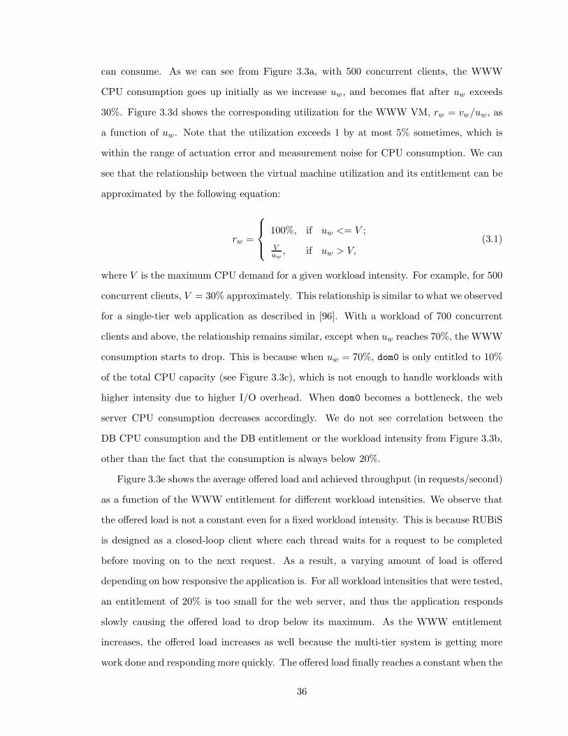
can consume. As we can see from Figure 3.3a, with 500 concurrent clients, the WWW
CPU consumption goes up initially as we increase uw, and becomes flat after uw exceeds
30%. Figure 3.3d shows the corresponding utilization for the WWW VM, rw = vw/uw, as
a function of uw. Note that the utilization exceeds 1 by at most 5% sometimes, which is
within the range of actuation error and measurement noise for CPU consumption. We can
see that the relationship between the virtual machine utilization and its entitlement can be
approximated by the following equation:
rw =
100%, if uw <= V ;
Vuw
, if uw > V,(3.1)
where V is the maximum CPU demand for a given workload intensity. For example, for 500
concurrent clients, V = 30% approximately. This relationship is similar to what we observed
for a single-tier web application as described in [96]. With a workload of 700 concurrent
clients and above, the relationship remains similar, except when uw reaches 70%, the WWW
consumption starts to drop. This is because when uw = 70%, dom0 is only entitled to 10%
of the total CPU capacity (see Figure 3.3c), which is not enough to handle workloads with
higher intensity due to higher I/O overhead. When dom0 becomes a bottleneck, the web
server CPU consumption decreases accordingly. We do not see correlation between the
DB CPU consumption and the DB entitlement or the workload intensity from Figure 3.3b,
other than the fact that the consumption is always below 20%.
Figure 3.3e shows the average offered load and achieved throughput (in requests/second)
as a function of the WWW entitlement for different workload intensities. We observe that
the offered load is not a constant even for a fixed workload intensity. This is because RUBiS
is designed as a closed-loop client where each thread waits for a request to be completed
before moving on to the next request. As a result, a varying amount of load is offered
depending on how responsive the application is. For all workload intensities that were tested,
an entitlement of 20% is too small for the web server, and thus the application responds
slowly causing the offered load to drop below its maximum. As the WWW entitlement
increases, the offered load increases as well because the multi-tier system is getting more
work done and responding more quickly. The offered load finally reaches a constant when the
36

0
5
10
15
20
25
30
35
20 30 40 50 60 70 80
Loss
(re
qs/s
ec)
WWW-I Entitlement (% of CPU)
Average Loss - IAverage Loss - II
(a) Loss
0
1
2
3
4
5
6
7
20 30 40 50 60 70 80
Res
pons
e T
ime
(sec
s)
WWW-I Entitlement (% of CPU)
Average RT - IAverage RT - II
(b) Response time
0 10 20 30 40 50 60 70 80 90
20 30 40 50 60 70 80
QoS
Rat
io (
norm
aliz
ed)
WWW-I entitlement (% of CPU)
Average Loss RatioAverage RT Ratio
(c) Loss ratio and RT ratio
Figure 3.4: Loss ratio and response time ratio for two RUBiS applications in the WS-DUscenario
web server is getting more than its need. Similarly, as the WWW entitlement is increased,
the throughput increases initially and then reaches a constant load. For a larger number of
clients (700 and above), we see a similar drop at uw = 70% in both the offered load and the
throughput because dom0 starts to become a bottleneck as discussed earlier. We also see a
significant loss (requests not completed) with a larger number of clients.
Figure 3.3f shows the average response time as a function of the WWW entitlement,
validating our observation on the throughput-entitlement relationship. As uw increases, re-
sponse time decreases initially reaching a minimum and then rises again at 70% entitlement
because of dom0 not getting enough CPU. We also note that the response time is roughly
inversely proportional to the throughput because of the closed-loop nature of the RUBiS
client.
37
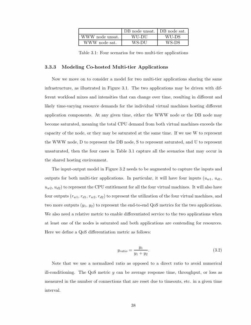
DB node unsat. DB node sat.
WWW node unsat. WU-DU WU-DS
WWW node sat. WS-DU WS-DS
Table 3.1: Four scenarios for two multi-tier applications
3.3.3 Modeling Co-hosted Multi-tier Applications
Now we move on to consider a model for two multi-tier applications sharing the same
infrastructure, as illustrated in Figure 3.1. The two applications may be driven with dif-
ferent workload mixes and intensities that can change over time, resulting in different and
likely time-varying resource demands for the individual virtual machines hosting different
application components. At any given time, either the WWW node or the DB node may
become saturated, meaning the total CPU demand from both virtual machines exceeds the
capacity of the node, or they may be saturated at the same time. If we use W to represent
the WWW node, D to represent the DB node, S to represent saturated, and U to represent
unsaturated, then the four cases in Table 3.1 capture all the scenarios that may occur in
the shared hosting environment.
The input-output model in Figure 3.2 needs to be augmented to capture the inputs and
outputs for both multi-tier applications. In particular, it will have four inputs (uw1, ud1,
uw2, ud2) to represent the CPU entitlement for all the four virtual machines. It will also have
four outputs (rw1, rd1, rw2, rd2) to represent the utilization of the four virtual machines, and
two more outputs (y1, y2) to represent the end-to-end QoS metrics for the two applications.
We also need a relative metric to enable differentiated service to the two applications when
at least one of the nodes is saturated and both applications are contending for resources.
Here we define a QoS differentiation metric as follows:
yratio =y1
y1 + y2. (3.2)
Note that we use a normalized ratio as opposed to a direct ratio to avoid numerical
ill-conditioning. The QoS metric y can be average response time, throughput, or loss as
measured in the number of connections that are reset due to timeouts, etc. in a given time
interval.
38

In the following subsections, we explain the relationship between the inputs (entitlement)
and the outputs (VM utilization and QoS) in all the four scenarios. We used two RUBiS
instances in WU-DU, WS-DU cases and two TPC-W instances in WU-DS case, because
the TPC-W clients stress the database more than the RUBiS clients.
3.3.3.1 WU-DU case
When neither the WWW node nor the DB node is saturated, the two applications can
have access to the shared resource as much as they need to. Therefore they can be viewed
as two independent applications as if they each had their own dedicated nodes. In this
case, the model we showed in Section 3.3.2 is applicable to each application and no QoS
differentiation metric is necessary. As a result, we can have a controller that controls the
resource entitlements for the two applications independently.
3.3.3.2 WS-DU case
This is the scenario where the WWW node is saturated but the DB node is unsaturated.
In this case, the CPU capacity of the WWW node cannot satisfy the needs of the two WWW
VMs simultaneously. Arbitration is required to decide how much CPU capacity each WWW
VM is entitled to based on a given QoS differentiation metric. We can either use a loss
ratio or a response time ratio as defined in equation (3.2) as the differentiation metric.
Figures 3.4a and 3.4b show the average loss (number of connections reset per second)
and average response time (seconds) for two RUBiS applications as a function of the WWW
entitlement (percentage) for application 1 (uw1). Note that uw2 = 1 − uw1. Figure 3.4c
shows the normalized loss ratio and response time ratio between the two applications as a
function of uw1.
As we can see from Figure 3.4a, as the first WWW entitlement increases, the loss
experienced by clients of both applications first increases and then decreases, resulting in
a non-monotonic relationship between the loss ratio and uw1 as evident from Figure 3.4c.
This is again due to the closed-loop nature of the RUBiS client where the offered load is
reduced as either of the application components becomes a bottleneck.
Figure 3.4b shows a different behavior for response time, where the response time for
39
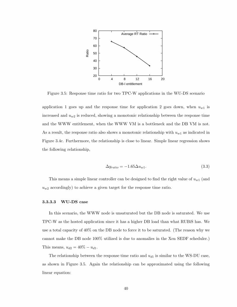
20
30
40
50
60
70
80
0 4 8 12 16 20
Rat
ioDB-I entitlement
Average RT Ratio
Figure 3.5: Response time ratio for two TPC-W applications in the WU-DS scenario
application 1 goes up and the response time for application 2 goes down, when uw1 is
increased and uw2 is reduced, showing a monotonic relationship between the response time
and the WWW entitlement, when the WWW VM is a bottleneck and the DB VM is not.
As a result, the response ratio also shows a monotonic relationship with uw1 as indicated in
Figure 3.4c. Furthermore, the relationship is close to linear. Simple linear regression shows
the following relationship,
∆yratio = −1.65∆uw1. (3.3)
This means a simple linear controller can be designed to find the right value of uw1 (and
uw2 accordingly) to achieve a given target for the response time ratio.
3.3.3.3 WU-DS case
In this scenario, the WWW node is unsaturated but the DB node is saturated. We use
TPC-W as the hosted application since it has a higher DB load than what RUBiS has. We
use a total capacity of 40% on the DB node to force it to be saturated. (The reason why we
cannot make the DB node 100% utilized is due to anomalies in the Xen SEDF scheduler.)
This means, ud2 = 40%− ud1.
The relationship between the response time ratio and ud1 is similar to the WS-DU case,
as shown in Figure 3.5. Again the relationship can be approximated using the following
linear equation:
40
∆yratio = −2.75∆ud1. (3.4)
Again, a simple linear controller can be designed to manage the response time ratio
between the two applications.
3.3.3.4 WS-DS case
We were unable to create this scenario in our testbed due to anomalies in the Xen
SEDF scheduler. The problem is pronounced with the capping option in scheduling (which
provides us with an actuator). Whenever capping is enabled, we always ran into very low
CPU consumption on WWW VMs which resulted in low consumption in the DB VMs
as well. After various experiments, we concluded that the problem lies in how the Xen
scheduler handles capping in the context of I/O-intensive applications.
3.4 Controller Design
In order to achieve the controller objectives outlined in Section 3.4, we designed a two-
layered architecture for the controller, as illustrated in Figure 3.6.
The first layer consists of four independent controllers, each of which can be viewed as
an “agent” for each of the four virtual machines, w1, w2, d1, d2. The role of these agents is
to compute the required CPU entitlement (ureq) for each virtual machine such that, 1) the
hosted application component gets enough resource so that it does not become a bottleneck
in the multi-tier application; 2) the virtual machine maintains a relatively high resource
utilization. In our design, the way to achieve these goals is to maintain a specified level of
utilization in each virtual machine. Therefore, the first layer controllers are referred to as
utilization controllers (UCs). We describe how the utilization controllers work in Section
3.4.1.
The second layer controller works on behalf of the shared nodes and serves as an “ar-
biter” that determines whether the requested CPU entitlements (ureq) for all of the virtual
machines can be satisfied, and if not, decides the final CPU entitlement (u) for each VM
41
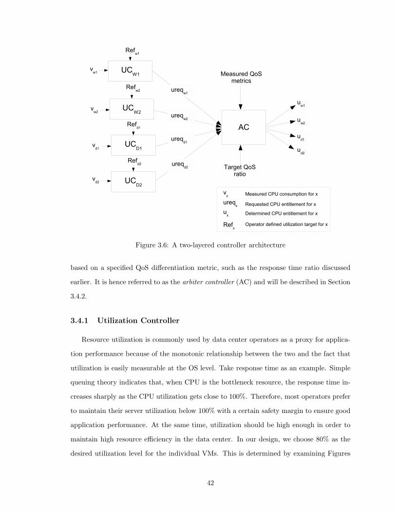
Figure 3.6: A two-layered controller architecture
based on a specified QoS differentiation metric, such as the response time ratio discussed
earlier. It is hence referred to as the arbiter controller (AC) and will be described in Section
3.4.2.
3.4.1 Utilization Controller
Resource utilization is commonly used by data center operators as a proxy for applica-
tion performance because of the monotonic relationship between the two and the fact that
utilization is easily measurable at the OS level. Take response time as an example. Simple
queuing theory indicates that, when CPU is the bottleneck resource, the response time in-
creases sharply as the CPU utilization gets close to 100%. Therefore, most operators prefer
to maintain their server utilization below 100% with a certain safety margin to ensure good
application performance. At the same time, utilization should be high enough in order to
maintain high resource efficiency in the data center. In our design, we choose 80% as the
desired utilization level for the individual VMs. This is determined by examining Figures
42

Adaptive
ControllerContainer
rref e u
v
rd
Workload
−
Figure 3.7: Adaptive utilization controller
3.3d, 3.3e and 3.3f together, which show that both the response time and the throughput
are at an acceptable level when the utilization of the bottleneck tier, the WWW VM, stays
below this target.
We have developed an adaptive integral controller in [96] for dynamic sizing of a virtual
machine based on its consumption such that the relative utilization of the VM can be
maintained in spite of the changing demand. The block diagram for the controller is shown
in Figure 3.7. At the beginning of the control interval k, the controller takes as inputs the
desired utilization (rref ) and the measured consumption during the previous interval (v(k−
1)). The controller computes the utilization of the VM (r) as r(k − 1) = v(k − 1)/u(k − 1)
and the tracking error (e) as e(k−1) = rref −r(k−1), and decides the resource entitlement
(u) for the VM for the next interval.
This controller is applied in our work as the utilization controllers in the first layer of
our controller architecture. For each VM, the UC calculates the required CPU entitlement
(ureq) using the following control law:
ureq(k) = ureq(k − 1)−K(k)e(k − 1). (3.5)
The integral gain parameter K(k) determines how aggressive the controller is in correct-
ing the observed error. The value of K(k) adapts automatically to the varying workload
by calculating K(k) = λ ∗ v(k − 1)/rref , where λ is a tunable constant. Compared to a
standard integral controller that has a fixed K value, our adaptive integral controller with
43
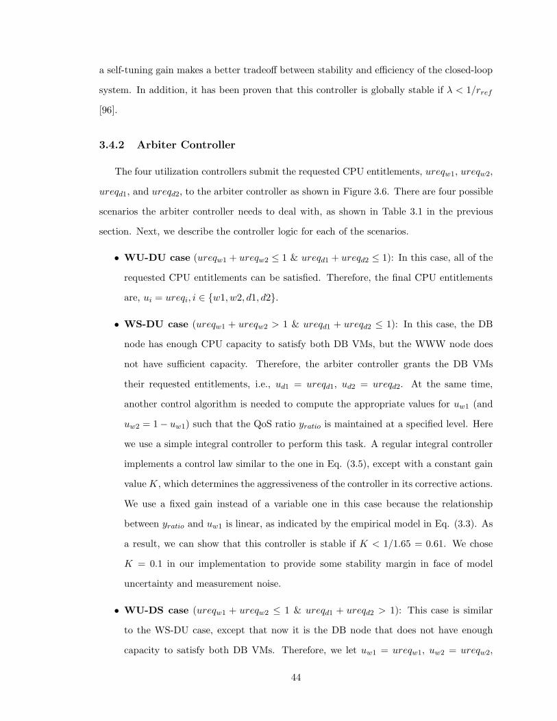
a self-tuning gain makes a better tradeoff between stability and efficiency of the closed-loop
system. In addition, it has been proven that this controller is globally stable if λ < 1/rref
[96].
3.4.2 Arbiter Controller
The four utilization controllers submit the requested CPU entitlements, ureqw1, ureqw2,
ureqd1, and ureqd2, to the arbiter controller as shown in Figure 3.6. There are four possible
scenarios the arbiter controller needs to deal with, as shown in Table 3.1 in the previous
section. Next, we describe the controller logic for each of the scenarios.
• WU-DU case (ureqw1 + ureqw2 ≤ 1 & ureqd1 + ureqd2 ≤ 1): In this case, all of the
requested CPU entitlements can be satisfied. Therefore, the final CPU entitlements
are, ui = ureqi, i ∈ {w1, w2, d1, d2}.
• WS-DU case (ureqw1 + ureqw2 > 1 & ureqd1 + ureqd2 ≤ 1): In this case, the DB
node has enough CPU capacity to satisfy both DB VMs, but the WWW node does
not have sufficient capacity. Therefore, the arbiter controller grants the DB VMs
their requested entitlements, i.e., ud1 = ureqd1, ud2 = ureqd2. At the same time,
another control algorithm is needed to compute the appropriate values for uw1 (and
uw2 = 1− uw1) such that the QoS ratio yratio is maintained at a specified level. Here
we use a simple integral controller to perform this task. A regular integral controller
implements a control law similar to the one in Eq. (3.5), except with a constant gain
value K, which determines the aggressiveness of the controller in its corrective actions.
We use a fixed gain instead of a variable one in this case because the relationship
between yratio and uw1 is linear, as indicated by the empirical model in Eq. (3.3). As
a result, we can show that this controller is stable if K < 1/1.65 = 0.61. We chose
K = 0.1 in our implementation to provide some stability margin in face of model
uncertainty and measurement noise.
• WU-DS case (ureqw1 + ureqw2 ≤ 1 & ureqd1 + ureqd2 > 1): This case is similar
to the WS-DU case, except that now it is the DB node that does not have enough
capacity to satisfy both DB VMs. Therefore, we let uw1 = ureqw1, uw2 = ureqw2,
44
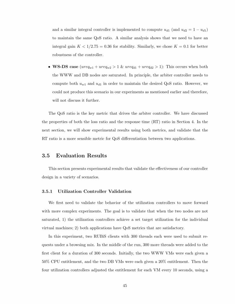
and a similar integral controller is implemented to compute ud1 (and ud2 = 1 − ud1)
to maintain the same QoS ratio. A similar analysis shows that we need to have an
integral gain K < 1/2.75 = 0.36 for stability. Similarly, we chose K = 0.1 for better
robustness of the controller.
• WS-DS case (ureqw1 + ureqw2 > 1 & ureqd1 + ureqd2 > 1): This occurs when both
the WWW and DB nodes are saturated. In principle, the arbiter controller needs to
compute both uw1 and ud1 in order to maintain the desired QoS ratio. However, we
could not produce this scenario in our experiments as mentioned earlier and therefore,
will not discuss it further.
The QoS ratio is the key metric that drives the arbiter controller. We have discussed
the properties of both the loss ratio and the response time (RT) ratio in Section 4. In the
next section, we will show experimental results using both metrics, and validate that the
RT ratio is a more sensible metric for QoS differentiation between two applications.
3.5 Evaluation Results
This section presents experimental results that validate the effectiveness of our controller
design in a variety of scenarios.
3.5.1 Utilization Controller Validation
We first need to validate the behavior of the utilization controllers to move forward
with more complex experiments. The goal is to validate that when the two nodes are not
saturated, 1) the utilization controllers achieve a set target utilization for the individual
virtual machines; 2) both applications have QoS metrics that are satisfactory.
In this experiment, two RUBiS clients with 300 threads each were used to submit re-
quests under a browsing mix. In the middle of the run, 300 more threads were added to the
first client for a duration of 300 seconds. Initially, the two WWW VMs were each given a
50% CPU entitlement, and the two DB VMs were each given a 20% entitlement. Then the
four utilization controllers adjusted the entitlement for each VM every 10 seconds, using a
45
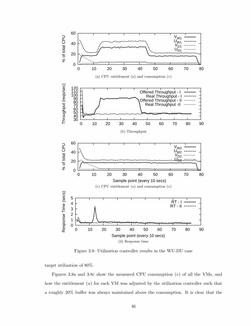
0
20
40
60
0 10 20 30 40 50 60 70 80%
of t
otal
CP
U VW1UW1VD1UD1
(a) CPU entitlement (u) and consumption (v)
30 40 50 60 70 80 90
100 110 120
0 10 20 30 40 50 60 70 80 90Thr
ough
put (
reqs
/sec
)
Offered Throughput - I Real Throughput - I
Offered Throughput - IIReal Throughput -II
(b) Throughput
0
20
40
60
0 10 20 30 40 50 60 70 80
% o
f tot
al C
PU
Sample point (every 10 secs)
VW2UW2VD2UD2
(c) CPU entitlement (u) and consumption (v)
0 1 2 3 4 5
0 10 20 30 40 50 60 70 80 90Res
pons
e T
ime
(sec
s)
Sample point (every 10 secs)
RT - IRT - II
(d) Response time
Figure 3.8: Utilization controller results in the WU-DU case
target utilization of 80%.
Figures 3.8a and 3.8c show the measured CPU consumption (v) of all the VMs, and
how the entitlement (u) for each VM was adjusted by the utilization controller such that
a roughly 20% buffer was always maintained above the consumption. It is clear that the
46
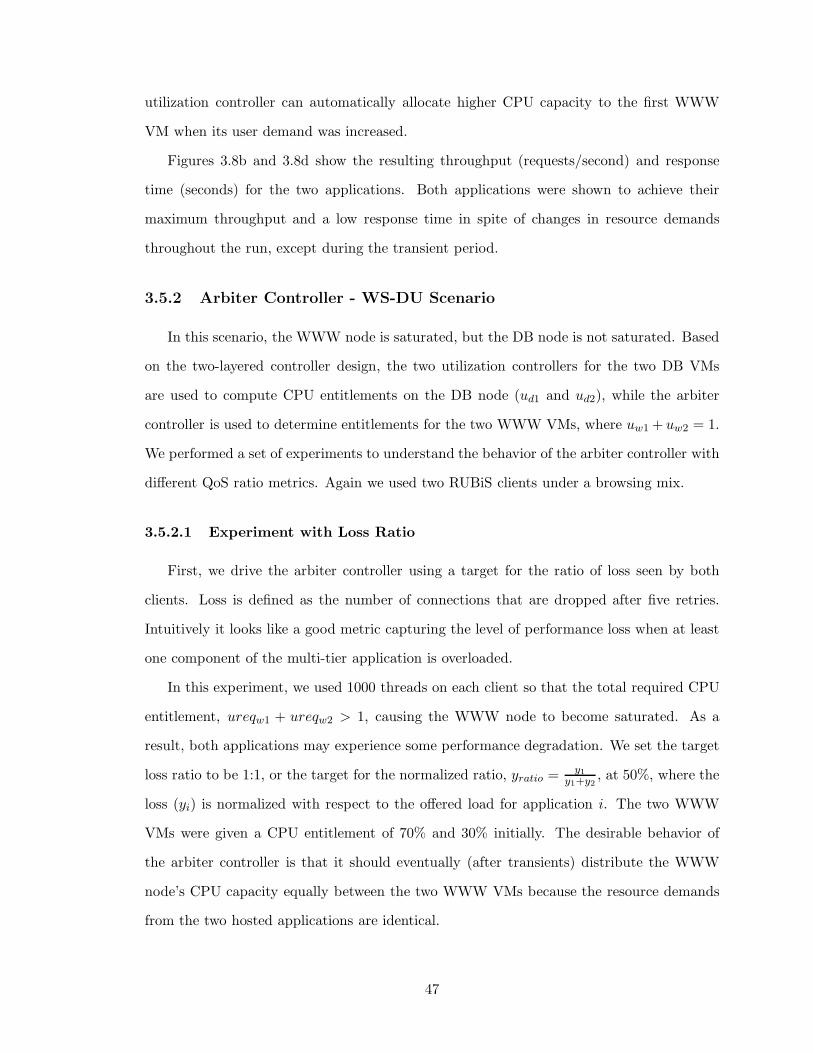
utilization controller can automatically allocate higher CPU capacity to the first WWW
VM when its user demand was increased.
Figures 3.8b and 3.8d show the resulting throughput (requests/second) and response
time (seconds) for the two applications. Both applications were shown to achieve their
maximum throughput and a low response time in spite of changes in resource demands
throughout the run, except during the transient period.
3.5.2 Arbiter Controller - WS-DU Scenario
In this scenario, the WWW node is saturated, but the DB node is not saturated. Based
on the two-layered controller design, the two utilization controllers for the two DB VMs
are used to compute CPU entitlements on the DB node (ud1 and ud2), while the arbiter
controller is used to determine entitlements for the two WWW VMs, where uw1 + uw2 = 1.
We performed a set of experiments to understand the behavior of the arbiter controller with
different QoS ratio metrics. Again we used two RUBiS clients under a browsing mix.
3.5.2.1 Experiment with Loss Ratio
First, we drive the arbiter controller using a target for the ratio of loss seen by both
clients. Loss is defined as the number of connections that are dropped after five retries.
Intuitively it looks like a good metric capturing the level of performance loss when at least
one component of the multi-tier application is overloaded.
In this experiment, we used 1000 threads on each client so that the total required CPU
entitlement, ureqw1 + ureqw2 > 1, causing the WWW node to become saturated. As a
result, both applications may experience some performance degradation. We set the target
loss ratio to be 1:1, or the target for the normalized ratio, yratio = y1
y1+y2, at 50%, where the
loss (yi) is normalized with respect to the offered load for application i. The two WWW
VMs were given a CPU entitlement of 70% and 30% initially. The desirable behavior of
the arbiter controller is that it should eventually (after transients) distribute the WWW
node’s CPU capacity equally between the two WWW VMs because the resource demands
from the two hosted applications are identical.
47
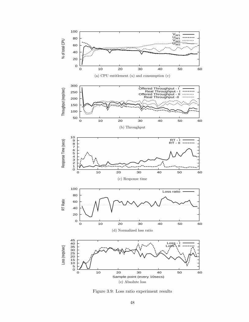
0
20
40
60
80
100
0 10 20 30 40 50 60
% o
f tot
al C
PU
VW1UW1VW2UW2
(a) CPU entitlement (u) and consumption (v)
50
100
150
200
250
300
0 10 20 30 40 50 60
Thro
ughp
ut (r
eqs/s
ec) Offered Throughput - I
Real Throughput - IOffered Throughput - II
Real Throughput -II
(b) Throughput
0 1 2 3 4 5 6 7 8 9
10
0 10 20 30 40 50 60
Resp
onse
Tim
e (s
ecs) RT - I
RT - II
(c) Response time
0
20
40
60
80
100
0 10 20 30 40 50 60
RT R
atio
Loss ratio
(d) Normalized loss ratio
0 5
10 15 20 25 30 35 40 45
0 10 20 30 40 50 60
Loss
(req
s/sec
)
Sample point (every 10secs)
Loss - ILoss - II
(e) Absolute loss
Figure 3.9: Loss ratio experiment results
48
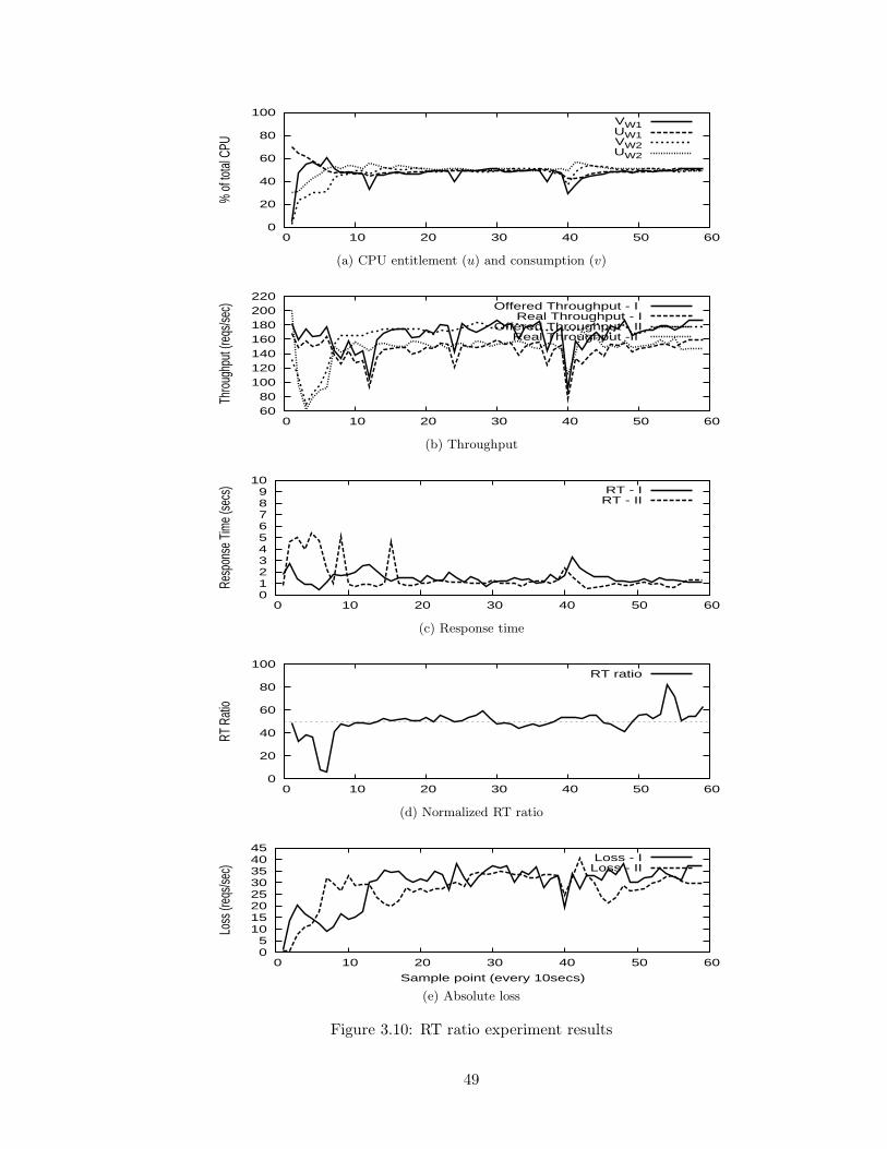
0
20
40
60
80
100
0 10 20 30 40 50 60%
of t
otal
CPU
VW1UW1VW2UW2
(a) CPU entitlement (u) and consumption (v)
60 80
100 120 140 160 180 200 220
0 10 20 30 40 50 60
Thro
ughp
ut (r
eqs/s
ec) Offered Throughput - I
Real Throughput - IOffered Throughput - II
Real Throughput -II
(b) Throughput
0 1 2 3 4 5 6 7 8 9
10
0 10 20 30 40 50 60
Resp
onse
Tim
e (s
ecs) RT - I
RT - II
(c) Response time
0
20
40
60
80
100
0 10 20 30 40 50 60
RT R
atio
RT ratio
(d) Normalized RT ratio
0 5
10 15 20 25 30 35 40 45
0 10 20 30 40 50 60
Loss
(req
s/sec
)
Sample point (every 10secs)
Loss - ILoss - II
(e) Absolute loss
Figure 3.10: RT ratio experiment results
49
Figure 3.9a shows the measured CPU consumption (vw1 and vw2) and the CPU entitle-
ment (uw1 and uw2) determined by the arbiter controller for the two WWW VMs. Figures
3.9b and 3.9c show the resulting throughput and response time for the two applications.
Figures 3.9d and 3.9e show the the normalized loss ratio (yratio) and absolute loss (re-
quests/second) seen by the two clients. As we can see, although the normalized loss ratio
was maintained around 50%, as time progressed, the second WWW VM was actually re-
ceiving higher and higher CPU entitlement over time. As a result, application 2 was able
to deliver much better throughput and response time compared to application 1.
This behavior is highly undesirable. It can be explained by revisiting Figure 3.4c in
Section 3.3. Because the relationship between the loss ratio and the entitlement is not
monotonic, any given target loss ratio can either be unachievable (if too high or too low), or
may have more than one equilibrium. This means that a loss ratio of 1:1 can be achieved not
only when uw1 = uw2, but also when uw1 6= uw2. This again is due to the closed-loop nature
of the RUBiS client. A slight disturbance in the CPU entitlement can cause one client to
submit less load thus getting less throughput. However, the normalized loss seen by this
client may still be equal to that of the other client, resulting in the loss ratio maintained at
1:1, and the controller cannot see the erratic behavior. This problem can be fixed by using
the response time ratio as the QoS differentiation metric.
3.5.2.2 Experiments with RT Ratio
Figures 3.10a, 3.10b, 3.10c, 3.10d, 3.10e show the results using the RT ratio as the
driving metric for the arbiter controller. The remaining test conditions were kept the
same, and an RT ratio of 1:1 was used. Here, we see very desirable behavior where the
arbiter controller grants equal entitlements to the CPU capacity between the two WWW
VMs. Consequently, the two multi-tier applications achieve fairly comparable performance
in terms of throughput and response time. Comparison between this result and the result
from the previous experiment shows that the RT ratio is a fairer metric than the loss ratio to
be used for QoS differentiation among co-hosted applications. One natural question around
this subject is, why not use a throughput ratio instead? The answer is two-fold. First,
for a closed-loop client, response time is on average inversely proportional to throughput
50
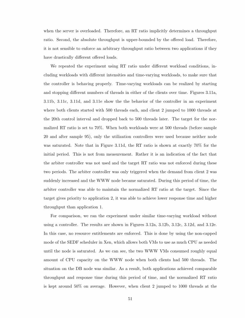
when the server is overloaded. Therefore, an RT ratio implicitly determines a throughput
ratio. Second, the absolute throughput is upper-bounded by the offered load. Therefore,
it is not sensible to enforce an arbitrary throughput ratio between two applications if they
have drastically different offered loads.
We repeated the experiment using RT ratio under different workload conditions, in-
cluding workloads with different intensities and time-varying workloads, to make sure that
the controller is behaving properly. Time-varying workloads can be realized by starting
and stopping different numbers of threads in either of the clients over time. Figures 3.11a,
3.11b, 3.11c, 3.11d, and 3.11e show the the behavior of the controller in an experiment
where both clients started with 500 threads each, and client 2 jumped to 1000 threads at
the 20th control interval and dropped back to 500 threads later. The target for the nor-
malized RT ratio is set to 70%. When both workloads were at 500 threads (before sample
20 and after sample 95), only the utilization controllers were used because neither node
was saturated. Note that in Figure 3.11d, the RT ratio is shown at exactly 70% for the
initial period. This is not from measurement. Rather it is an indication of the fact that
the arbiter controller was not used and the target RT ratio was not enforced during these
two periods. The arbiter controller was only triggered when the demand from client 2 was
suddenly increased and the WWW node became saturated. During this period of time, the
arbiter controller was able to maintain the normalized RT ratio at the target. Since the
target gives priority to application 2, it was able to achieve lower response time and higher
throughput than application 1.
For comparison, we ran the experiment under similar time-varying workload without
using a controller. The results are shown in Figures 3.12a, 3.12b, 3.12c, 3.12d, and 3.12e.
In this case, no resource entitlements are enforced. This is done by using the non-capped
mode of the SEDF scheduler in Xen, which allows both VMs to use as much CPU as needed
until the node is saturated. As we can see, the two WWW VMs consumed roughly equal
amount of CPU capacity on the WWW node when both clients had 500 threads. The
situation on the DB node was similar. As a result, both applications achieved comparable
throughput and response time during this period of time, and the normalized RT ratio
is kept around 50% on average. However, when client 2 jumped to 1000 threads at the
51
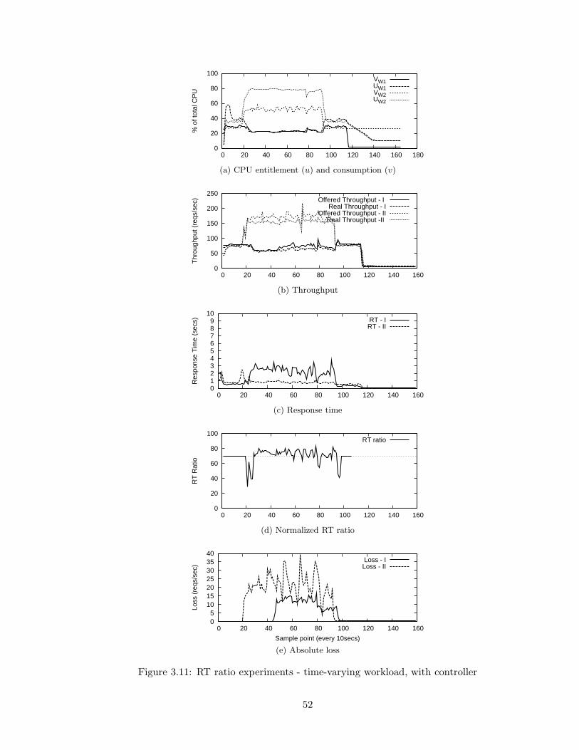
0
20
40
60
80
100
0 20 40 60 80 100 120 140 160 180
% o
f tot
al C
PU
VW1UW1VW2UW2
(a) CPU entitlement (u) and consumption (v)
0
50
100
150
200
250
0 20 40 60 80 100 120 140 160
Thr
ough
put (
reqs
/sec
) Offered Throughput - I Real Throughput - I
Offered Throughput - IIReal Throughput -II
(b) Throughput
0 1 2 3 4 5 6 7 8 9
10
0 20 40 60 80 100 120 140 160
Res
pons
e T
ime
(sec
s) RT - IRT - II
(c) Response time
0
20
40
60
80
100
0 20 40 60 80 100 120 140 160
RT
Rat
io
RT ratio
(d) Normalized RT ratio
0 5
10 15 20 25 30 35 40
0 20 40 60 80 100 120 140 160
Loss
(re
qs/s
ec)
Sample point (every 10secs)
Loss - ILoss - II
(e) Absolute loss
Figure 3.11: RT ratio experiments - time-varying workload, with controller
52

0
20
40
60
80
100
0 10 20 30 40 50 60 70 80 90 100
% o
f tot
al C
PU
Vw1Vw2Vd1Vd2
(a) CPU entitlement (u) and consumption (v)
0
50
100
150
200
0 10 20 30 40 50 60 70 80 90 100
Thr
ough
put (
reqs
/sec
) Offered Throughput -I Real Throughput -I
Offered Throughput -I Real Throughput - II
(b) Throughput
0 1 2 3 4 5 6 7 8 9
10
0 10 20 30 40 50 60 70 80 90 100
Res
pons
e tim
e (s
ecs) RT - I
RT - II
(c) Response time
0
20
40
60
80
100
0 10 20 30 40 50 60 70 80 90 100
Res
pons
e tim
e ra
tio
RT Ratio
(d) Normalized RT ratio
0
0.5
1
1.5
2
0 10 20 30 40 50 60 70 80 90 100
Loss
(re
qs/s
ec)
Loss - ILoss - II
(e) Absolute loss
Figure 3.12: RT ratio experiments - time-varying workload, without controller
53
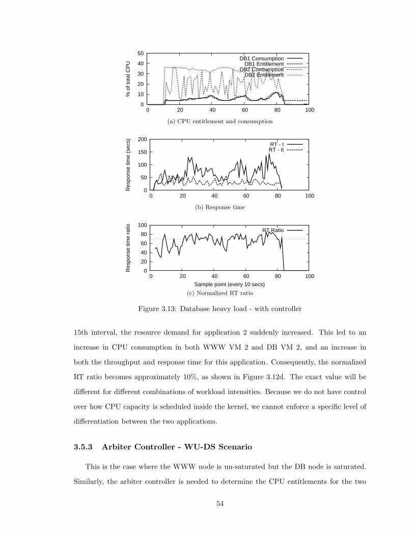
0
10
20
30
40
50
0 20 40 60 80 100
% o
f tot
al C
PU
DB1 ConsumptionDB1 Entitlement
DB2 ConsumptionDB2 Entitlement
(a) CPU entitlement and consumption
0
50
100
150
200
0 20 40 60 80 100
Res
pons
e tim
e (s
ecs)
RT - IRT - II
(b) Response time
0
20
40
60
80
100
0 20 40 60 80 100
Res
pons
e tim
e ra
tio
Sample point (every 10 secs)
RT Ratio
(c) Normalized RT ratio
Figure 3.13: Database heavy load - with controller
15th interval, the resource demand for application 2 suddenly increased. This led to an
increase in CPU consumption in both WWW VM 2 and DB VM 2, and an increase in
both the throughput and response time for this application. Consequently, the normalized
RT ratio becomes approximately 10%, as shown in Figure 3.12d. The exact value will be
different for different combinations of workload intensities. Because we do not have control
over how CPU capacity is scheduled inside the kernel, we cannot enforce a specific level of
differentiation between the two applications.
3.5.3 Arbiter Controller - WU-DS Scenario
This is the case where the WWW node is un-saturated but the DB node is saturated.
Similarly, the arbiter controller is needed to determine the CPU entitlements for the two
54
0
10
20
30
40
50
10080604020
% o
f tot
al C
PU
DB I ConsumptionDB II Consumption
(a) CPU consumption for two DB VMs
0 20 40 60 80
100 120 140
10080604020
Res
pons
e tim
e (s
ecs)
RT - IRT - II
(b) Response time
0
20
40
60
80
100
10080604020
Res
pons
e tim
e ra
tio
Sample point (every 10 secs)
RT Ratio
(c) Normalized RT ratio
Figure 3.14: Database heavy load - without controller
DB VMs. We tested our controller by using two instances of the TPC-W benchmark as the
two applications. A shopping mix was used to generate the client requests in order to place
more stress on the DB tier. Since the total DB load does not go up to 100%, we capped the
sum of ud1 and ud2 at 40% in order to create the WU-DS scenario for testing our controller.
Again, a target RT ratio of 70% was used.
We tested the controller against different workload combinations. An example is shown
in Figures 3.13a, 3.13b, and 3.13c where two TPC-W clients each with 300 threads were
used. The arbiter controller was able to maintain the normalized RT ratio around the target,
but with more oscillation than was present in the WS-DU case. This can be explained by
inspecting the measured CPU consumption and response time over time. Both metrics
show a great deal of variation, indicating the greater burstiness of a DB-intensive workload
55
compared to a web-intensive workload. It is also shown in the larger scaling factor in Eq.
(3.4) compared to Eq. (3.3), indicating a higher sensitivity of the response time with respect
to a small change in the entitlement. In spite of the noise in the various metrics, application
2 did receive better QoS from the system in general, as driven by the RT ratio for service
differentiation.
Again, for comparison, we ran the experiment under the same workload condition with-
out using a controller. The results are shown in Figures 3.14a, 3.14b, and 3.14c. As we can
see, the CPU capacity of the DB node was shared roughly equally between the two DB VMs
resulting in comparable average response time for the two applications. Figure 3.14c shows
the resulting RT ratio oscillating around an average value of 50%. This result re-confirms
that, without a feedback-driven resource controller, we cannot provide QoS differentiation
between the two applications at a specified level when the system is overloaded.
3.6 Summary
In this work, we built a testbed for a data center hosting multiple multi-tier applications
using virtualization. We have developed a two-layered controller using classical control
theory. The controller algorithms were designed based on input-output models inferred
from empirical data using a black-box approach. The controller was tested in various
scenarios including stressing the web and the database tier separately. The experimental
results confirmed that our controller design achieves high utilization of the data center while
meeting application-level QoS goals. Moreover, it is able to provide a specified level of QoS
differentiation between applications under overload conditions, which cannot be obtained
under standard OS-level scheduling that is not QoS-driven.
We still see space for improvement in controller performance, in terms of better stability
and responsiveness, especially for DB intensive workloads. In this work, only fixed models
were used to capture the input-output relationship in the steady state, which simplifies both
the modeling process and the controller design. In the next chapter, we explore the use of
a dynamic model to capture more transient behavior of the system and use it as the basis
for better controller design. We also want to explore the effect of VM migration on our
56
controller.
We would like to extend our work to control sharing of memory, disk I/O, and network
resources. These resources pose unique challenges as sharing I/O resources usually involves
sharing of related buffers in the kernel as well. Currently, the virtualization technologies do
a poor job of providing control of sharing and isolation of I/O resources. With the advent
of I/O virtualization technologies from CPU vendors, this may change and we would like
to apply our algorithms to take full advantage of the new hardware capabilities.
In the next chapter, we describe a multi resource controller that uses an adpative online
model and can control multiple resources.
57
CHAPTER 4
Multi-resource Controller
4.1 Introduction
In this chapter, we address the problem of managing the allocation of computational
resources in a shared, virtualized infrastructure to achieve application-level SLOs. Our
solution to this problem is AutoControl, an automated resource control and adaptation
system.
Our main contributions are twofold: First, we design an online model estimator to dy-
namically determine and capture the relationship between application level performance
and the allocation of individual resource shares. Our adaptive modeling approach captures
the complex behavior of enterprise applications including varying resource demands over
time, resource demands from distributed application components, and shifting demands
across multiple resources types. Second, we design a two-layered, multi-input, multi-output
(MIMO) controller to automatically allocate multiple types of resources to multiple en-
terprise applications to achieve their SLOs. The first layer consists of a set of application
controllers that automatically determines the amount of resources necessary to achieve indi-
vidual application SLOs, using the estimated models and a feedback approach. The second
layer is comprised of a set of node controllers that detect resource bottlenecks on the shared
nodes and properly allocate resources of multiple types to individual applications. In over-
load cases, the node controllers can provide service differentiation by prioritizing allocation
among different applications.
58
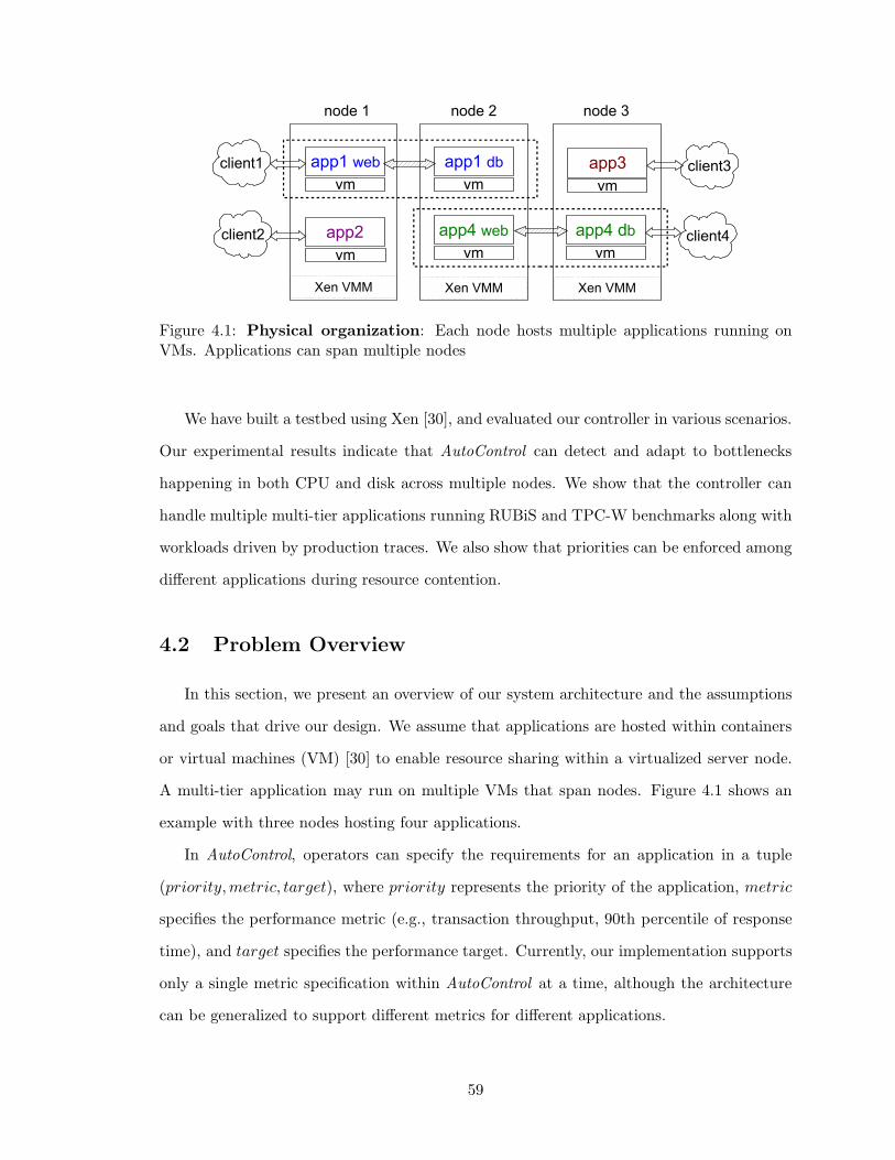
Figure 4.1: Physical organization: Each node hosts multiple applications running onVMs. Applications can span multiple nodes
We have built a testbed using Xen [30], and evaluated our controller in various scenarios.
Our experimental results indicate that AutoControl can detect and adapt to bottlenecks
happening in both CPU and disk across multiple nodes. We show that the controller can
handle multiple multi-tier applications running RUBiS and TPC-W benchmarks along with
workloads driven by production traces. We also show that priorities can be enforced among
different applications during resource contention.
4.2 Problem Overview
In this section, we present an overview of our system architecture and the assumptions
and goals that drive our design. We assume that applications are hosted within containers
or virtual machines (VM) [30] to enable resource sharing within a virtualized server node.
A multi-tier application may run on multiple VMs that span nodes. Figure 4.1 shows an
example with three nodes hosting four applications.
In AutoControl, operators can specify the requirements for an application in a tuple
(priority,metric, target), where priority represents the priority of the application, metric
specifies the performance metric (e.g., transaction throughput, 90th percentile of response
time), and target specifies the performance target. Currently, our implementation supports
only a single metric specification within AutoControl at a time, although the architecture
can be generalized to support different metrics for different applications.
59
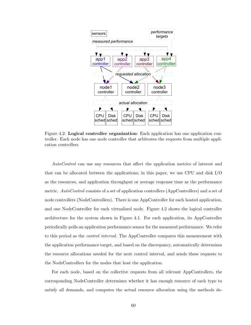
Figure 4.2: Logical controller organization: Each application has one application con-troller. Each node has one node controller that arbitrates the requests from multiple appli-cation controllers
AutoControl can use any resources that affect the application metrics of interest and
that can be allocated between the applications; in this paper, we use CPU and disk I/O
as the resources, and application throughput or average response time as the performance
metric. AutoControl consists of a set of application controllers (AppControllers) and a set of
node controllers (NodeControllers). There is one AppController for each hosted application,
and one NodeController for each virtualized node. Figure 4.2 shows the logical controller
architecture for the system shown in Figure 4.1. For each application, its AppController
periodically polls an application performance sensor for the measured performance. We refer
to this period as the control interval. The AppController compares this measurement with
the application performance target, and based on the discrepancy, automatically determines
the resource allocations needed for the next control interval, and sends these requests to
the NodeControllers for the nodes that host the application.
For each node, based on the collective requests from all relevant AppControllers, the
corresponding NodeController determines whether it has enough resource of each type to
satisfy all demands, and computes the actual resource allocation using the methods de-
60

scribed in Section 4.3. The computed allocation values are fed into the resource schedulers
in the virtualization layer for actuation, which allocate the corresponding portions of the
node resources to the VMs in real time. Figure 4.2 shows CPU and disk schedulers as
examples.
The AutoControl architecture allows the placement of AppControllers and NodeCon-
trollers in a distributed fashion. NodeControllers can be hosted in the physical node they
are controlling. AppControllers can be hosted in a node where one of the application tiers
is located. We do not mandate this placement, however, and the data center operator can
choose to host a set of controllers in a node dedicated for control operations.
We assume that all nodes in the data center are connected with a high speed network,
so that sensor and actuation delays within AutoControl are small compared to the control
interval. We also require accurate system sensors and actuators, and assume that the
underlying system schedulers provide a rich enough interface to dynamically adjust resource
shares for VMs.
We set the following goals in designing AutoControl :
Performance assurance: If all applications can meet their performance targets, Auto-
Control should allocate resources properly to achieve them. If they cannot be met,
AutoControl should provide service differentiation according to application priorities.
Automation: While performance targets and certain parameters within AutoControl may
be set manually, all allocation decisions should be made automatically without human
intervention.
Adaptation: The controller should adapt to variations in workloads or system conditions.
Scalability: The controller architecture should scale to a large environment with many
applications and nodes by not requiring a single centralized controller.
4.3 Controller Design
This section details the design of both AppController and NodeController in the two-
layered architecture of AutoControl. For easy reference, Table 4.1 summarizes the mathe-
61
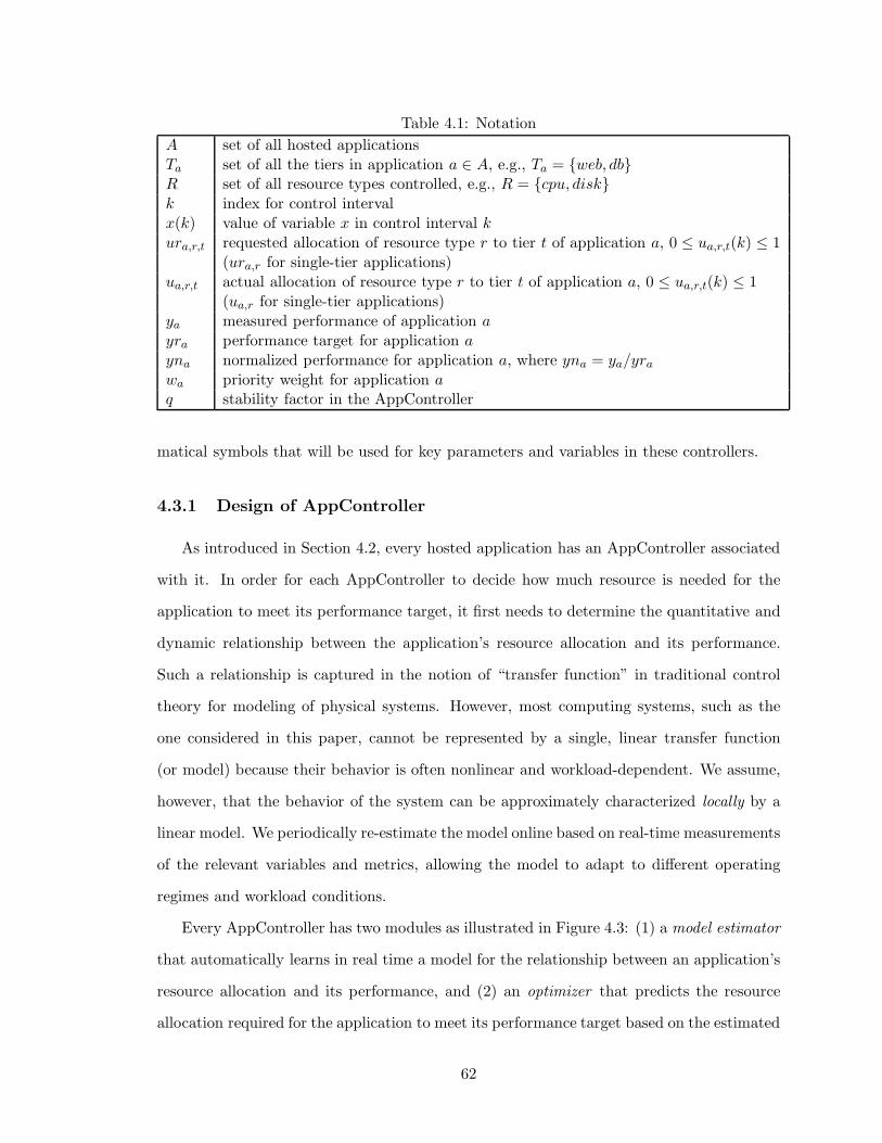
Table 4.1: Notation
A set of all hosted applicationsTa set of all the tiers in application a ∈ A, e.g., Ta = {web, db}R set of all resource types controlled, e.g., R = {cpu, disk}k index for control intervalx(k) value of variable x in control interval kura,r,t requested allocation of resource type r to tier t of application a, 0 ≤ ua,r,t(k) ≤ 1
(ura,r for single-tier applications)ua,r,t actual allocation of resource type r to tier t of application a, 0 ≤ ua,r,t(k) ≤ 1
(ua,r for single-tier applications)ya measured performance of application ayra performance target for application ayna normalized performance for application a, where yna = ya/yra
wa priority weight for application aq stability factor in the AppController
matical symbols that will be used for key parameters and variables in these controllers.
4.3.1 Design of AppController
As introduced in Section 4.2, every hosted application has an AppController associated
with it. In order for each AppController to decide how much resource is needed for the
application to meet its performance target, it first needs to determine the quantitative and
dynamic relationship between the application’s resource allocation and its performance.
Such a relationship is captured in the notion of “transfer function” in traditional control
theory for modeling of physical systems. However, most computing systems, such as the
one considered in this paper, cannot be represented by a single, linear transfer function
(or model) because their behavior is often nonlinear and workload-dependent. We assume,
however, that the behavior of the system can be approximately characterized locally by a
linear model. We periodically re-estimate the model online based on real-time measurements
of the relevant variables and metrics, allowing the model to adapt to different operating
regimes and workload conditions.
Every AppController has two modules as illustrated in Figure 4.3: (1) a model estimator
that automatically learns in real time a model for the relationship between an application’s
resource allocation and its performance, and (2) an optimizer that predicts the resource
allocation required for the application to meet its performance target based on the estimated
62

Figure 4.3: AppController’s internal structure
model. For each application a ∈ A, let ya(k) be the value of its performance metric provided
by an application performance sensor at the end of control interval k, and let yra be the
desired value for its performance. Furthermore, we define yna(k) = ya(k)/yra to be the
normalized performance value for interval k. We then define the resource-allocation variable
ua to be a vector that contains all the elements in the set {ua,r,t : r ∈ R, t ∈ Ta}. For
example, for a two-tier application whose performance depends on two critical resources,
e.g., Ta = {web, db} and R = {cpu, disk}, ua is a 4-dimensional vector. ua(k) represents
the resource-allocation values for application a during interval k (we represent all vectors
in boldface).
4.3.1.1 Model Estimator
For every control interval, the model estimator re-computes a linear model that ap-
proximates the nonlinear and time-varying relationship between the resource allocation to
application a (ua) and its normalized performance (yna) around the current operating point.
More specifically, the following auto-regressive-moving-average (ARMA) model is used to
represent this relationship:
yna(k) = a1(k) yna(k − 1) + a2(k) yna(k − 2)
+b0T (k)ua(k) + b1
T (k)ua(k − 1), (4.1)
63
where the model parameters a1(k) and a2(k) capture the correlation between the applica-
tion’s past and present performance, and b0(k) and b1(k) are vectors of coefficients cap-
turing the correlation between the current performance and the recent resource allocations.
Both ua(k) and ua(k− 1) are column vectors, and b0T (k) and b1
T (k) are row vectors. We
chose a linear model because it is easy to estimate online and simplifies the corresponding
controller design problem. In our experiments, we have found that the second-order ARMA
model in Eq. (4.1) (i.e., one that takes into account the past two control intervals) can
predict the application performance with adequate accuracy. (Some evidence of this will be
presented later in Section 4.6.) Note that the model developed may not be unique because
of the adaptive nature, but is sufficient to allocate resources to meet application goals.
The reason why we model the normalized performance rather than the absolute per-
formance is that the latter can have an arbitrary magnitude. The normalized performance
yna has values that are comparable to those of the resource allocations in ua, which are less
than 1. This improves the numerical stability of the algorithm.
Note that the model represented in Eq. (4.1) is adaptive itself, because all the model
parameters a1, a2, b0 and b1 are functions of time interval k. These parameters can be
re-estimated online using the recursive least squares (RLS) method [28]. At the end of every
control interval k − 1, the model estimator collects the newly-measured performance value
ya(k − 1), normalizes it by the performance target yra, and uses it to update the values
for the model parameters. The approach assumes that drastic variations in workloads that
cause significant model parameter changes occur infrequently relative to the control interval,
thus allowing the the model estimator to converge locally around an operating point and
track changes in the operating point. The recursive nature of RLS makes the time taken
for this computation negligible for control intervals longer than 10 seconds.
4.3.1.2 Optimizer
The main goal of the optimizer is to determine the resource allocation required (ura) in
order for the application to meet its target performance. An additional goal is to accomplish
this in a stable manner, without causing large oscillations in the resource allocation. We
64
achieve these goals by finding the value of ura that minimizes the following cost function:
Ja = (yna(k)− 1)2 + q‖ura(k)− ua(k − 1)‖2. (4.2)
To explain the intuition behind this function, we define Jp = (yna(k) − 1)2, and Jc =
‖ura(k)−ua(k−1)‖2. It is easy to see that Jp is 0 when ya(k) = yra, i.e., when application
a is meeting its performance target. Otherwise, Jp serves as a penalty for the deviation of
the application’s measured performance from its target. Therefore, we refer to Jp as the
performance cost.
The second function Jc, referred to as the control cost, is included to improve controller
stability. The value of Jc is higher when the controller makes a larger change in the resource
allocation in a single interval. Because Ja = Jp + q · Jc, our controller aims to minimize a
linear combination of both the performance cost and the control cost. Using the approximate
linear relationship between the normalized performance and the resource allocation, as
described by Eq. (4.1), we can derive the resource allocation required to minimize the cost
function Ja, in terms of the recent resource allocation ua and the corresponding normalized
performance values yna:
ur∗a(k) = (b0b0T + qI)−1((1− a1 yna(k − 1)
−a2 yna(k − 2)− b1Tua(k − 1))b0 + qua(k − 1)). (4.3)
This is a special case of the optimal control law derived in [63]. Note that the dependency
of the model parameters a1, a2, b0 and b1 on the control interval k has been dropped from
the equation to improve its readability.
To understand the intuition behind this control law and the effect of the scaling factor
q, we define ∆yna(k) = 1 − a1 yna(k − 1) − a2 yna(k − 2) − b1Tua(k − 1). This indicates
the discrepancy between the model-predicted value for yna(k) and its target (which is 1)
that needs to be compensated by the next allocation (ua(k)). For a small q value, ur∗a(k)
is dominated by the effect of ∆yna(k), and the controller reacts aggressively to tracking
errors in performance. As the value of q increases, ur∗a(k) is increasingly dominated by the
65
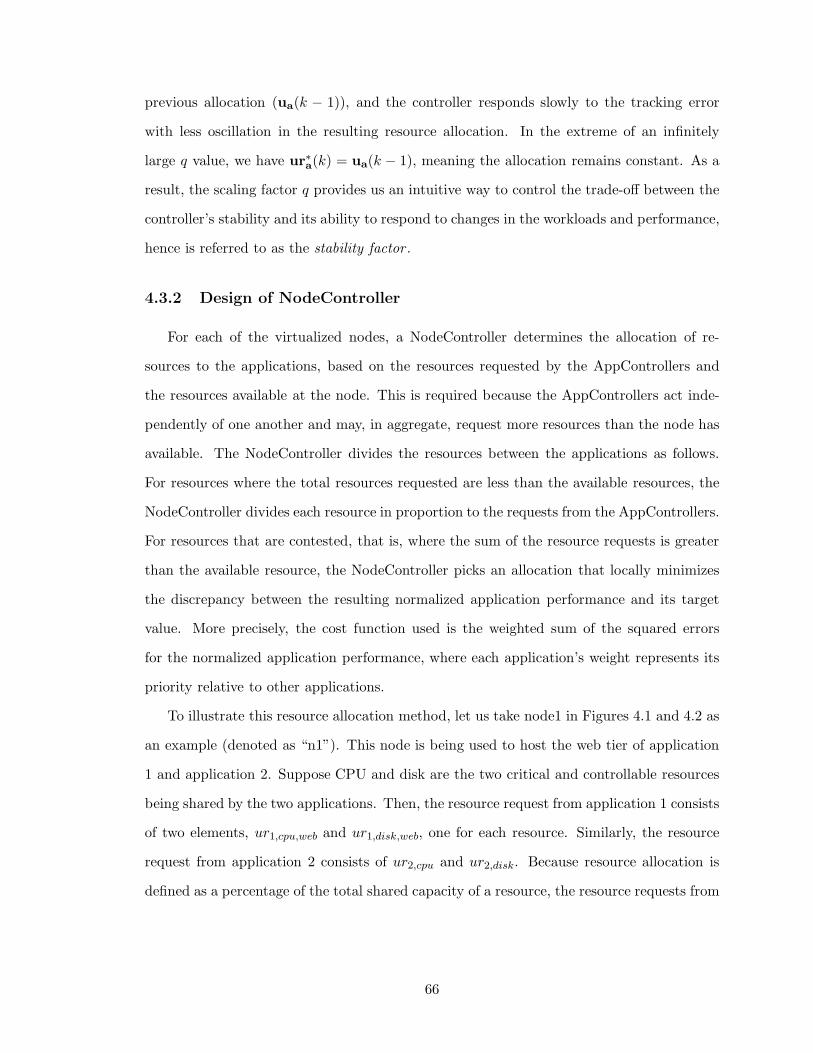
previous allocation (ua(k − 1)), and the controller responds slowly to the tracking error
with less oscillation in the resulting resource allocation. In the extreme of an infinitely
large q value, we have ur∗a(k) = ua(k − 1), meaning the allocation remains constant. As a
result, the scaling factor q provides us an intuitive way to control the trade-off between the
controller’s stability and its ability to respond to changes in the workloads and performance,
hence is referred to as the stability factor .
4.3.2 Design of NodeController
For each of the virtualized nodes, a NodeController determines the allocation of re-
sources to the applications, based on the resources requested by the AppControllers and
the resources available at the node. This is required because the AppControllers act inde-
pendently of one another and may, in aggregate, request more resources than the node has
available. The NodeController divides the resources between the applications as follows.
For resources where the total resources requested are less than the available resources, the
NodeController divides each resource in proportion to the requests from the AppControllers.
For resources that are contested, that is, where the sum of the resource requests is greater
than the available resource, the NodeController picks an allocation that locally minimizes
the discrepancy between the resulting normalized application performance and its target
value. More precisely, the cost function used is the weighted sum of the squared errors
for the normalized application performance, where each application’s weight represents its
priority relative to other applications.
To illustrate this resource allocation method, let us take node1 in Figures 4.1 and 4.2 as
an example (denoted as “n1”). This node is being used to host the web tier of application
1 and application 2. Suppose CPU and disk are the two critical and controllable resources
being shared by the two applications. Then, the resource request from application 1 consists
of two elements, ur1,cpu,web and ur1,disk,web, one for each resource. Similarly, the resource
request from application 2 consists of ur2,cpu and ur2,disk. Because resource allocation is
defined as a percentage of the total shared capacity of a resource, the resource requests from
66
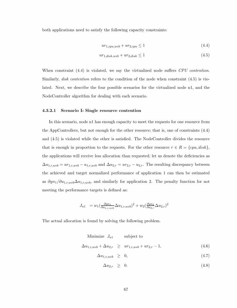
both applications need to satisfy the following capacity constraints:
ur1,cpu,web + ur2,cpu ≤ 1 (4.4)
ur1,disk,web + ur2,disk ≤ 1 (4.5)
When constraint (4.4) is violated, we say the virtualized node suffers CPU contention.
Similarly, disk contention refers to the condition of the node when constraint (4.5) is vio-
lated. Next, we describe the four possible scenarios for the virtualized node n1, and the
NodeController algorithm for dealing with each scenario.
4.3.2.1 Scenario I: Single resource contention
In this scenario, node n1 has enough capacity to meet the requests for one resource from
the AppControllers, but not enough for the other resource; that is, one of constraints (4.4)
and (4.5) is violated while the other is satisfied. The NodeController divides the resource
that is enough in proportion to the requests. For the other resource r ∈ R = {cpu, disk},
the applications will receive less allocation than requested; let us denote the deficiencies as
∆u1,r,web = ur1,r,web − u1,r,web and ∆u2,r = ur2,r − u2,r. The resulting discrepancy between
the achieved and target normalized performance of application 1 can then be estimated
as ∂yn1/∂u1,r,web∆u1,r,web, and similarly for application 2. The penalty function for not
meeting the performance targets is defined as:
Jn1 = w1(∂yn1
∂u1,r,web∆u1,r,web)
2 + w2(∂yn2
∂u2,r∆u2,r)
2
The actual allocation is found by solving the following problem.
Minimize Jn1 subject to
∆u1,r,web + ∆u2,r ≥ ur1,r,web + ur2,r − 1, (4.6)
∆u1,r,web ≥ 0, (4.7)
∆u2,r ≥ 0. (4.8)
67
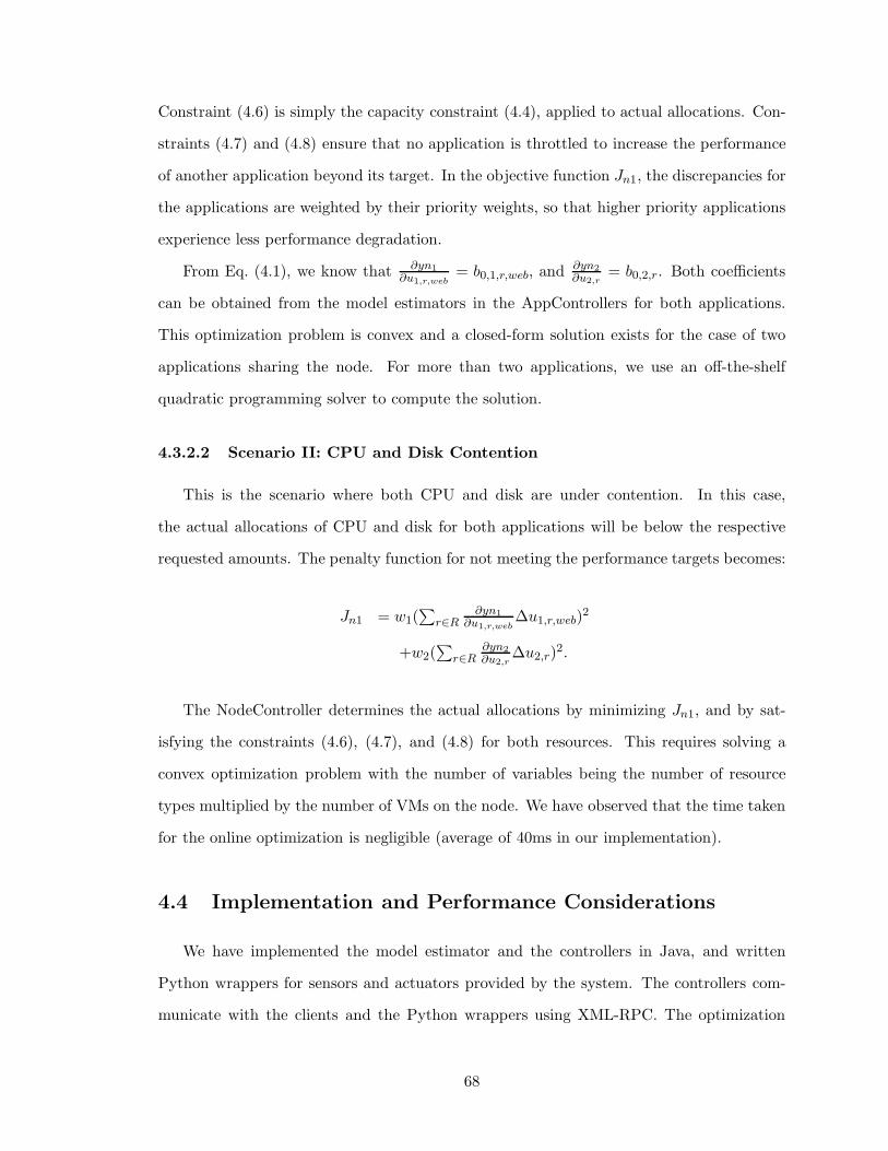
Constraint (4.6) is simply the capacity constraint (4.4), applied to actual allocations. Con-
straints (4.7) and (4.8) ensure that no application is throttled to increase the performance
of another application beyond its target. In the objective function Jn1, the discrepancies for
the applications are weighted by their priority weights, so that higher priority applications
experience less performance degradation.
From Eq. (4.1), we know that ∂yn1
∂u1,r,web= b0,1,r,web, and ∂yn2
∂u2,r= b0,2,r. Both coefficients
can be obtained from the model estimators in the AppControllers for both applications.
This optimization problem is convex and a closed-form solution exists for the case of two
applications sharing the node. For more than two applications, we use an off-the-shelf
quadratic programming solver to compute the solution.
4.3.2.2 Scenario II: CPU and Disk Contention
This is the scenario where both CPU and disk are under contention. In this case,
the actual allocations of CPU and disk for both applications will be below the respective
requested amounts. The penalty function for not meeting the performance targets becomes:
Jn1 = w1(∑
r∈R∂yn1
∂u1,r,web∆u1,r,web)
2
+w2(∑
r∈R∂yn2
∂u2,r∆u2,r)
2.
The NodeController determines the actual allocations by minimizing Jn1, and by sat-
isfying the constraints (4.6), (4.7), and (4.8) for both resources. This requires solving a
convex optimization problem with the number of variables being the number of resource
types multiplied by the number of VMs on the node. We have observed that the time taken
for the online optimization is negligible (average of 40ms in our implementation).
4.4 Implementation and Performance Considerations
We have implemented the model estimator and the controllers in Java, and written
Python wrappers for sensors and actuators provided by the system. The controllers com-
municate with the clients and the Python wrappers using XML-RPC. The optimization
68
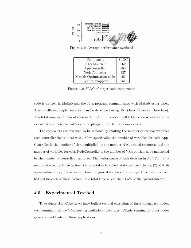
0
0.2
0.4
0.6
Tim
e (s
ec)
Perf stats sensingOptimization
CPU ActuationDisk Actuation
Total
Figure 4.4: Average performance overhead
Component SLOC
RLS Modeler 262AppController 280NodeController 327
Matlab Optimization code 35Python wrappers 251
Figure 4.5: SLOC of major code components
code is written in Matlab and the Java program communicates with Matlab using pipes.
A more efficient implementation can be developed using JNI (Java Native call Interface).
The total number of lines of code in AutoControl is about 3000. Our code is written to be
extensible and new controllers can be plugged into the framework easily.
The controllers are designed to be scalable by limiting the number of control variables
each controller has to deal with. More specifically, the number of variables for each App-
Controller is the number of tiers multiplied by the number of controlled resources, and the
number of variables for each NodeController is the number of VMs on that node multiplied
by the number of controlled resources. The performance of each decision in AutoControl is
mainly affected by three factors: (1) time taken to collect statistics from clients, (2) Matlab
optimization time, (3) actuation time. Figure 4.4 shows the average time taken on our
testbed for each of these factors. The total time is less than 1.5% of the control interval.
4.5 Experimental Testbed
To evaluate AutoControl, we have built a testbed consisting of three virtualized nodes,
each running multiple VMs hosting multiple applications. Clients running on other nodes
generate workloads for these applications.
69
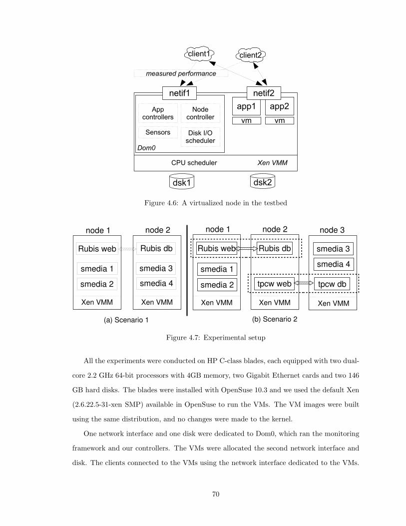
Figure 4.6: A virtualized node in the testbed
Figure 4.7: Experimental setup
All the experiments were conducted on HP C-class blades, each equipped with two dual-
core 2.2 GHz 64-bit processors with 4GB memory, two Gigabit Ethernet cards and two 146
GB hard disks. The blades were installed with OpenSuse 10.3 and we used the default Xen
(2.6.22.5-31-xen SMP) available in OpenSuse to run the VMs. The VM images were built
using the same distribution, and no changes were made to the kernel.
One network interface and one disk were dedicated to Dom0, which ran the monitoring
framework and our controllers. The VMs were allocated the second network interface and
disk. The clients connected to the VMs using the network interface dedicated to the VMs.
70

The controller used its own network interface to poll application performance statistics from
the clients. In order to demonstrate CPU bottlenecks more easily, we allocated one CPU
to the VMs, and used the remaining CPUs for Dom0. Our controller is fully extensible to
VMs sharing multiple processors as long as the CPU scheduler allows arbitrary slicing of
CPU allocation. Figure 4.6 shows all the components in our experiments.
Our experiments were designed to answer the following questions:
1. Can the controller detect resource bottlenecks across time and application tiers?
2. Can the controller adjust resource allocations to overcome these bottlenecks?
3. Can the controller handle different application workloads?
4. Can the controller enforce performance targets for metrics including average through-
put and response time?
5. Can the controller prioritize among applications when resources are scarce?
We used three different applications in our experiments: RUBiS [25], an online auction
site benchmark, a Java implementation of the TPC-W benchmark [34], and a custom-built
secure media server.
RUBiS and TPC-W use a multi-tier setup consisting of web and database tiers. They
both provide workloads of different mixes and time-varying intensity. For RUBiS, we used
a workload mix called the browsing mix that simulates a user browsing through an auction
site. For TPC-W, we used the shopping mix, which simulates a user browsing through a
shopping site. The browsing mix stresses the web tier, while the shopping mix exerts more
demand on the database tier.
The custom-built secure media (smedia) server is a representation of a media server that
can serve encrypted media streams. The smedia server runs a certain number of concurrent
threads, each serving a client that continuously requests media files from the server. A
media client can request an encrypted or unencrypted stream. Upon receiving the request,
the server reads the particular media file from the disk (or from memory if it is cached),
optionally encrypts it, and sends it to the client. A closed-loop client model is used where
a new file is only requested after the previous request is complete. Reading a file from
71

the disk consumes disk I/O resource, and encryption requires CPU resource. For a given
number of threads, by changing the fraction of the client requests for encrypted media, we
can vary the amount of CPU or disk I/O resource used. This flexibility allowed us to study
our controller’s behavior for CPU and disk I/O bottlenecks.
4.5.1 Simulating Production Traces
To test our controller under real workloads, we created workloads that simulate pro-
duction traces. These traces were obtained from an SAP application server running in a
production environment. We simulated the production traces using RUBiS and TPC-W by
carefully selecting the number of concurrent threads at a particular time. For example, to
create 40% average CPU utilization over a 5 minute period, we used 500 threads simulating
500 concurrent users. Note that we only simulated the CPU utilization of the production
trace. We did not attempt to recreate the disk utilization, because the traces did not contain
the needed metadata.
We also used traces generated from a media workload generator called MediSyn [88].
MediSyn generates traces that are based on analytical models drawn from real-world traces
collected at an HP Labs production media server. It captures important properties of
streaming media workloads, including file duration, popularity, encoding bit rate, and
streaming session time. We re-created the access pattern of the trace by closely follow-
ing the start times, end times, and bitrates of the sessions. Note that this is a re-creation
of the stochastics rather than replaying an original trace. We did not attempt to re-create
the disk access pattern, because of the lack of metadata.
4.5.2 Sensors
Our sensors periodically collect two types of statistics: real-time resource utilizations
and performance of applications. CPU utilization statistics are collected using Xen’s xm
command. Disk utilization statistics are collected using the iostat command, which is part
of the sysstat package. In our testbed, we measured both the application throughput and
the server-side response time directly from the application, where throughput is defined as
72
the total number of client requests serviced, and for each client request, response time is
defined as the amount of time taken to service the request. In a real data center, application-
level performance may be obtained from application logs or from tools like HP Openview.
4.5.3 Actuators
Our actuators included Xen’s credit-based CPU scheduler and a custom-built propor-
tional disk I/O scheduler. The credit scheduler provided by Xen allows each domain (or
VM) to be assigned a cap. We used the cap to specify a CPU share for each VM. This
non-work-conserving mode of CPU scheduling provided better performance isolation among
applications running in different VMs. The proportional share scheduler for disk I/O was
designed to maximize the efficiency of the disk access [48]. The scheduler is logically inter-
posed between the virtual machines and the physical disks: we implemented it as a driver
in the Dom0. The controller interacts with the disk I/O scheduler by assigning a share to
each VM in every control interval.
The controller interacts with the CPU scheduler by specifying a non-zero cap for each
VM in each control interval. Although the scheduler itself works in the non-work-conserving
mode, there is minimum waste of CPU cycles because the controller always allocates 100%
of the shared capacity to all the guest VMs, and because the controller automatically shifts
idle capacity from one VM to another by dynamically adapting the individual caps in
response to the changing needs of the individual applications.
4.6 Evaluation Results
We evaluated AutoControl in a number of experimental scenarios to answer the questions
posed in Section 4.5. In all of the experiments, a control interval of 20 seconds was used1. In
this section, we present the performance results from these experiments that demonstrate
the effectiveness of the AutoControl design.
1A higher interval may cause the controller to miss some dynamic changes, while a smaller interval maycause oscillations.
73

0
50
100
150
200
250
0 15 30 45 60 75 90
Thr
ough
put (
Req
uest
s/se
c)
Time intervals (every 20 secs)
CB DB CB
AutoControlwork-conserving
statictarget
(a) RUBiS throughput
0
100
200
300
400
500
600
700
800
0 15 30 45 60 75 90
Thr
ough
put (
Req
uest
s/se
c)
Time intervals (every 20 secs)
CB
DB
AutoControlwork-conserving
statictarget
(b) Smedia1 throughput
0
100
200
300
400
500
600
700
800
0 15 30 45 60 75 90
Thr
ough
put (
Req
uest
s/se
c)
Time intervals (every 20 secs)
CB
DB
AutoControlwork-conserving
statictarget
(c) Smedia2 throughput
0
100
200
300
400
500
600
700
800
0 15 30 45 60 75 90
Thr
ough
put (
Req
uest
s/se
c)
Time intervals (every 20 secs)
DB
CB
AutoControlwork-conserving
statictarget
(d) Smedia3 throughput
0
100
200
300
400
500
600
700
800
0 15 30 45 60 75 90
Thr
ough
put (
Req
uest
s/se
c)
Time intervals (every 20 secs)
DB
CB
AutoControlwork-conserving
statictarget
(e) Smedia4 throughput
Figure 4.8: Application throughput with bottlenecks in CPU or disk I/O and across multiplenodes
4.6.1 Scenario 1: Detecting and Mitigating Resource Bottlenecks in Mul-
tiple Resources and across Multiple Application Tiers
This scenario was designed to validate the following claims about AutoControl :
74
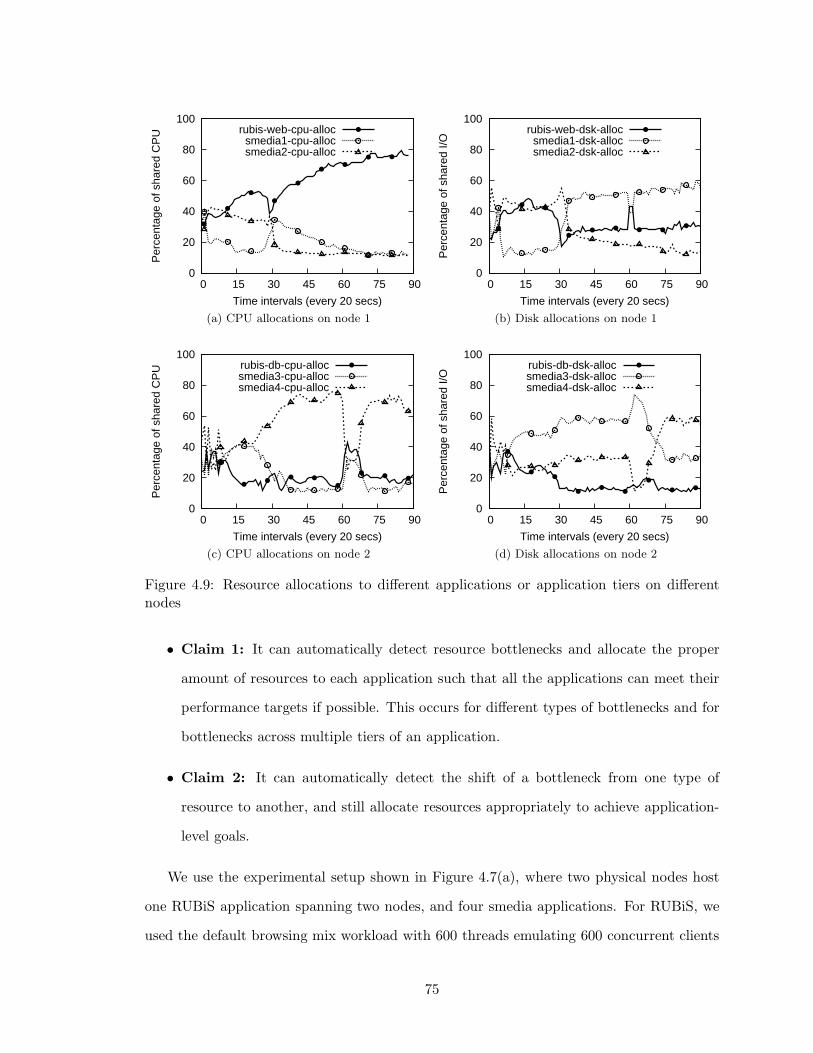
0
20
40
60
80
100
0 15 30 45 60 75 90
Per
cent
age
of s
hare
d C
PU
Time intervals (every 20 secs)
rubis-web-cpu-allocsmedia1-cpu-allocsmedia2-cpu-alloc
(a) CPU allocations on node 1
0
20
40
60
80
100
0 15 30 45 60 75 90
Per
cent
age
of s
hare
d I/O
Time intervals (every 20 secs)
rubis-web-dsk-allocsmedia1-dsk-allocsmedia2-dsk-alloc
(b) Disk allocations on node 1
0
20
40
60
80
100
0 15 30 45 60 75 90
Per
cent
age
of s
hare
d C
PU
Time intervals (every 20 secs)
rubis-db-cpu-allocsmedia3-cpu-allocsmedia4-cpu-alloc
(c) CPU allocations on node 2
0
20
40
60
80
100
0 15 30 45 60 75 90
Per
cent
age
of s
hare
d I/O
Time intervals (every 20 secs)
rubis-db-dsk-allocsmedia3-dsk-allocsmedia4-dsk-alloc
(d) Disk allocations on node 2
Figure 4.9: Resource allocations to different applications or application tiers on differentnodes
• Claim 1: It can automatically detect resource bottlenecks and allocate the proper
amount of resources to each application such that all the applications can meet their
performance targets if possible. This occurs for different types of bottlenecks and for
bottlenecks across multiple tiers of an application.
• Claim 2: It can automatically detect the shift of a bottleneck from one type of
resource to another, and still allocate resources appropriately to achieve application-
level goals.
We use the experimental setup shown in Figure 4.7(a), where two physical nodes host
one RUBiS application spanning two nodes, and four smedia applications. For RUBiS, we
used the default browsing mix workload with 600 threads emulating 600 concurrent clients
75
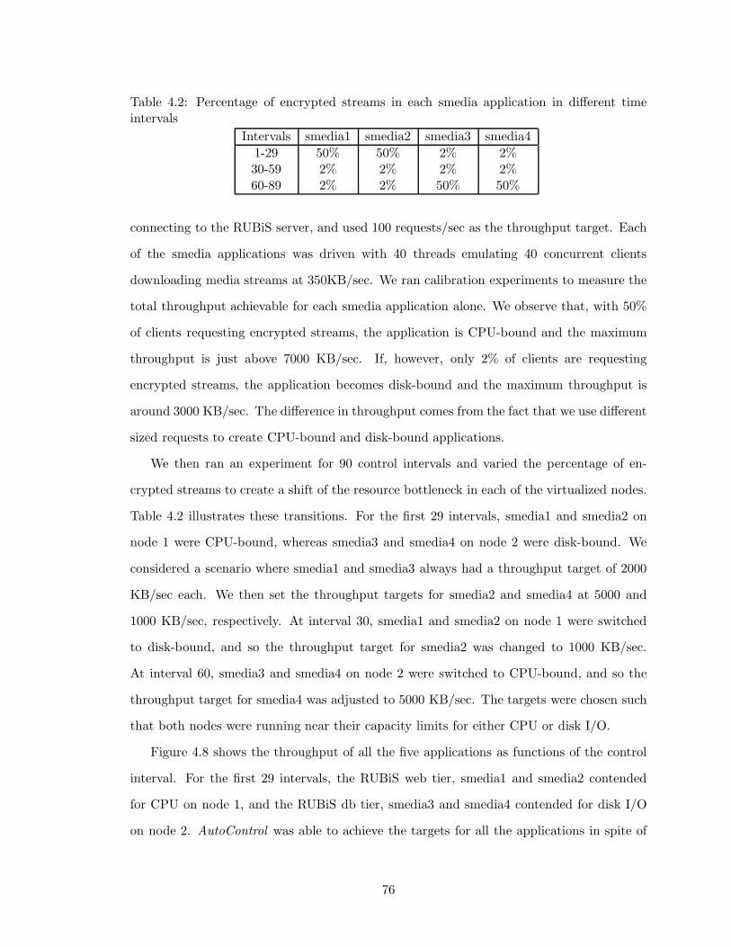
Table 4.2: Percentage of encrypted streams in each smedia application in different timeintervals
Intervals smedia1 smedia2 smedia3 smedia4
1-29 50% 50% 2% 2%30-59 2% 2% 2% 2%60-89 2% 2% 50% 50%
connecting to the RUBiS server, and used 100 requests/sec as the throughput target. Each
of the smedia applications was driven with 40 threads emulating 40 concurrent clients
downloading media streams at 350KB/sec. We ran calibration experiments to measure the
total throughput achievable for each smedia application alone. We observe that, with 50%
of clients requesting encrypted streams, the application is CPU-bound and the maximum
throughput is just above 7000 KB/sec. If, however, only 2% of clients are requesting
encrypted streams, the application becomes disk-bound and the maximum throughput is
around 3000 KB/sec. The difference in throughput comes from the fact that we use different
sized requests to create CPU-bound and disk-bound applications.
We then ran an experiment for 90 control intervals and varied the percentage of en-
crypted streams to create a shift of the resource bottleneck in each of the virtualized nodes.
Table 4.2 illustrates these transitions. For the first 29 intervals, smedia1 and smedia2 on
node 1 were CPU-bound, whereas smedia3 and smedia4 on node 2 were disk-bound. We
considered a scenario where smedia1 and smedia3 always had a throughput target of 2000
KB/sec each. We then set the throughput targets for smedia2 and smedia4 at 5000 and
1000 KB/sec, respectively. At interval 30, smedia1 and smedia2 on node 1 were switched
to disk-bound, and so the throughput target for smedia2 was changed to 1000 KB/sec.
At interval 60, smedia3 and smedia4 on node 2 were switched to CPU-bound, and so the
throughput target for smedia4 was adjusted to 5000 KB/sec. The targets were chosen such
that both nodes were running near their capacity limits for either CPU or disk I/O.
Figure 4.8 shows the throughput of all the five applications as functions of the control
interval. For the first 29 intervals, the RUBiS web tier, smedia1 and smedia2 contended
for CPU on node 1, and the RUBiS db tier, smedia3 and smedia4 contended for disk I/O
on node 2. AutoControl was able to achieve the targets for all the applications in spite of
76

the fact that (i) the resource bottleneck occurs either in the CPU or in the disk; (ii) both
tiers of the RUBiS application distributed across two physical nodes experienced resource
contention.
To help understand how the targets were achieved, Figures 4.9a and 4.9b show the CPU
and disk I/O allocations to the RUBiS web tier, smedia1 and smedia2 on node 1. For the
first 29 intervals, these three VMs were contending for CPU. The controller gave different
portions of both CPU and disk resources to the three VMs such that all of their targets
could be met. In the same time period (first 29 intervals), on node 2, the RUBiS database
tier, smedia3 and smedia4 were contending for the disk I/O. Figures 4.9c and 4.9d show
the CPU and disk I/O allocations for all the three VMs on this node. The controller not
only allocated the right proportion of disk I/O to smedia3 and smedia4 for them to achieve
their throughput targets, it also allocated the right amount of CPU to the RUBiS database
tier so that the two-tier application could meet its target.
At interval 30, the workloads for the smedia applications on node 1 were switched to be
disk-heavy. As a result, smedia1 and smedia2 were contending for disk I/O, since RUBiS
web tier uses minimal disk resource. The controller recognized this change in resource
bottleneck automatically and ensured that both smedia1 and smedia2 could meet their
new throughput targets by allocating the right amount of disk resources to both smedia
applications (see Figure 4.9b).
At interval 60, the workloads for the smedia applications on node 2 were switched to
be CPU-heavy. Because the RUBiS db tier also requires a non-negligible amount of CPU
(around 20%), smedia3 and smedia4 started contending for CPU with the RUBiS db tier
on node 2. Again, the controller was able to automatically translate the application-level
goals into appropriate resource allocations to the three VMs (see Figure 4.9c).
For comparison, we repeated the same experiment using two other resource allocation
methods that are commonly used on consolidated infrastructure, a work-conserving mode
and a static mode. In the work-conserving mode, the applications run in the default Xen
settings, where a cap of zero is specified for the shared CPU on a node, indicating that
the applications can use any amount of CPU resources. In this mode, our proportional
share disk scheduler was unloaded to allow unhindered disk access. In the static mode,
77
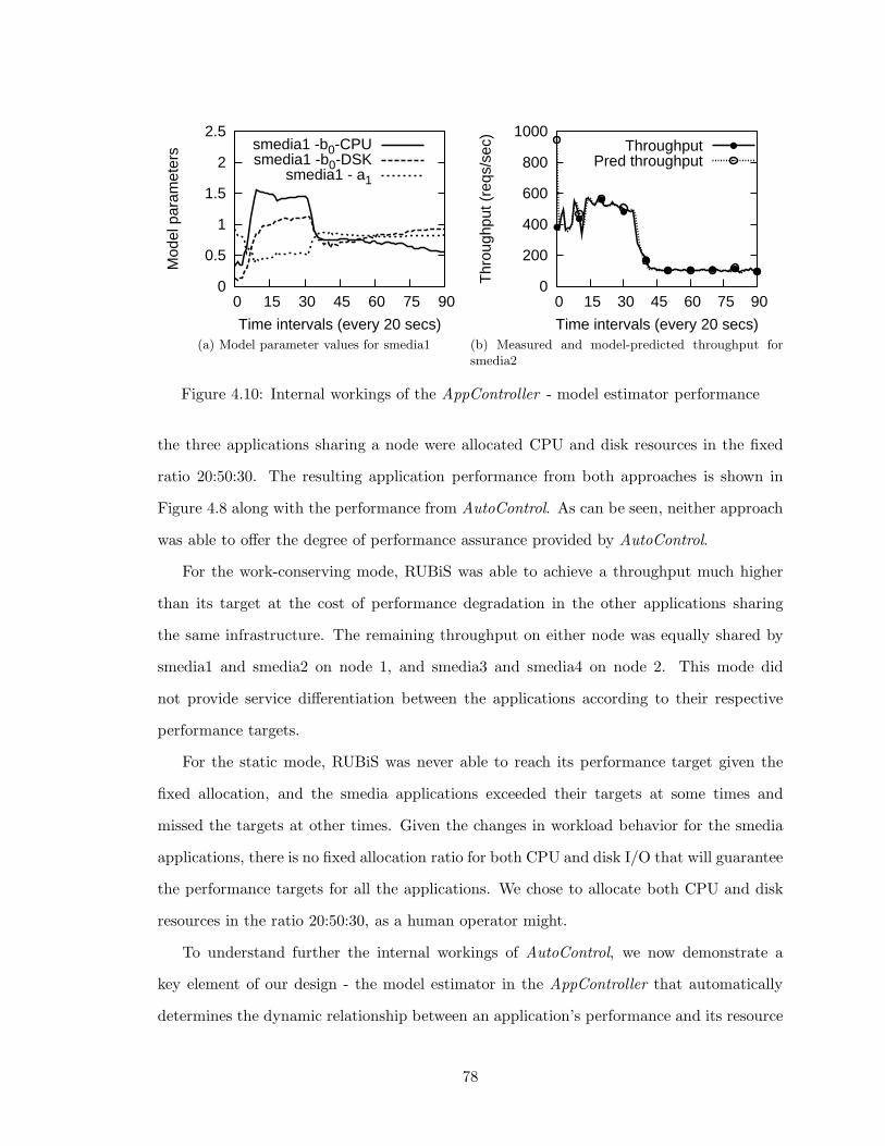
0
0.5
1
1.5
2
2.5
0 15 30 45 60 75 90
Mod
el p
aram
eter
s
Time intervals (every 20 secs)
smedia1 -b0-CPUsmedia1 -b0-DSK
smedia1 - a1
(a) Model parameter values for smedia1
0
200
400
600
800
1000
0 15 30 45 60 75 90
Thr
ough
put (
reqs
/sec
)
Time intervals (every 20 secs)
ThroughputPred throughput
(b) Measured and model-predicted throughput forsmedia2
Figure 4.10: Internal workings of the AppController - model estimator performance
the three applications sharing a node were allocated CPU and disk resources in the fixed
ratio 20:50:30. The resulting application performance from both approaches is shown in
Figure 4.8 along with the performance from AutoControl. As can be seen, neither approach
was able to offer the degree of performance assurance provided by AutoControl.
For the work-conserving mode, RUBiS was able to achieve a throughput much higher
than its target at the cost of performance degradation in the other applications sharing
the same infrastructure. The remaining throughput on either node was equally shared by
smedia1 and smedia2 on node 1, and smedia3 and smedia4 on node 2. This mode did
not provide service differentiation between the applications according to their respective
performance targets.
For the static mode, RUBiS was never able to reach its performance target given the
fixed allocation, and the smedia applications exceeded their targets at some times and
missed the targets at other times. Given the changes in workload behavior for the smedia
applications, there is no fixed allocation ratio for both CPU and disk I/O that will guarantee
the performance targets for all the applications. We chose to allocate both CPU and disk
resources in the ratio 20:50:30, as a human operator might.
To understand further the internal workings of AutoControl, we now demonstrate a
key element of our design - the model estimator in the AppController that automatically
determines the dynamic relationship between an application’s performance and its resource
78
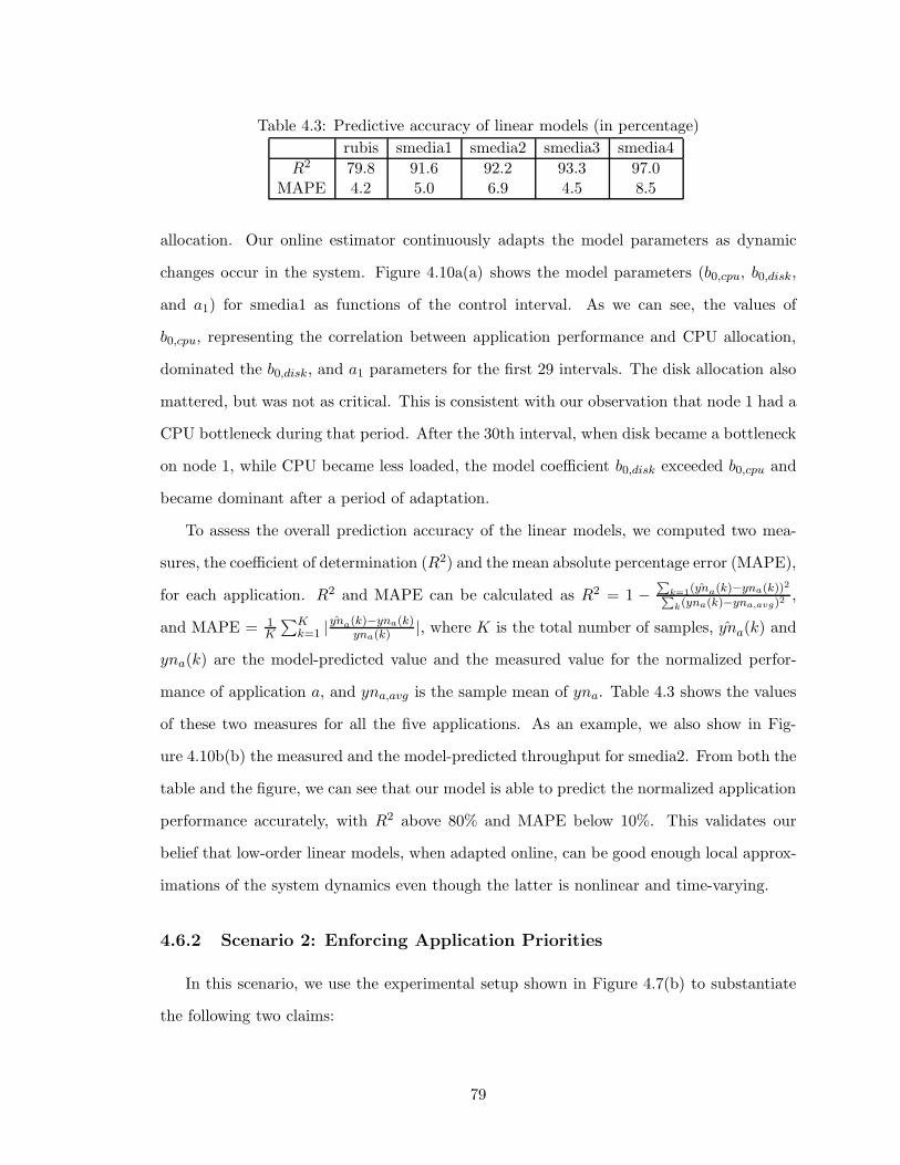
Table 4.3: Predictive accuracy of linear models (in percentage)
rubis smedia1 smedia2 smedia3 smedia4
R2 79.8 91.6 92.2 93.3 97.0MAPE 4.2 5.0 6.9 4.5 8.5
allocation. Our online estimator continuously adapts the model parameters as dynamic
changes occur in the system. Figure 4.10a(a) shows the model parameters (b0,cpu, b0,disk,
and a1) for smedia1 as functions of the control interval. As we can see, the values of
b0,cpu, representing the correlation between application performance and CPU allocation,
dominated the b0,disk, and a1 parameters for the first 29 intervals. The disk allocation also
mattered, but was not as critical. This is consistent with our observation that node 1 had a
CPU bottleneck during that period. After the 30th interval, when disk became a bottleneck
on node 1, while CPU became less loaded, the model coefficient b0,disk exceeded b0,cpu and
became dominant after a period of adaptation.
To assess the overall prediction accuracy of the linear models, we computed two mea-
sures, the coefficient of determination (R2) and the mean absolute percentage error (MAPE),
for each application. R2 and MAPE can be calculated as R2 = 1 −P
k=1(yna(k)−yna(k))2P
k(yna(k)−yna,avg)2,
and MAPE = 1K
∑Kk=1 |
yna(k)−yna(k)yna(k) |, where K is the total number of samples, yna(k) and
yna(k) are the model-predicted value and the measured value for the normalized perfor-
mance of application a, and yna,avg is the sample mean of yna. Table 4.3 shows the values
of these two measures for all the five applications. As an example, we also show in Fig-
ure 4.10b(b) the measured and the model-predicted throughput for smedia2. From both the
table and the figure, we can see that our model is able to predict the normalized application
performance accurately, with R2 above 80% and MAPE below 10%. This validates our
belief that low-order linear models, when adapted online, can be good enough local approx-
imations of the system dynamics even though the latter is nonlinear and time-varying.
4.6.2 Scenario 2: Enforcing Application Priorities
In this scenario, we use the experimental setup shown in Figure 4.7(b) to substantiate
the following two claims:
79
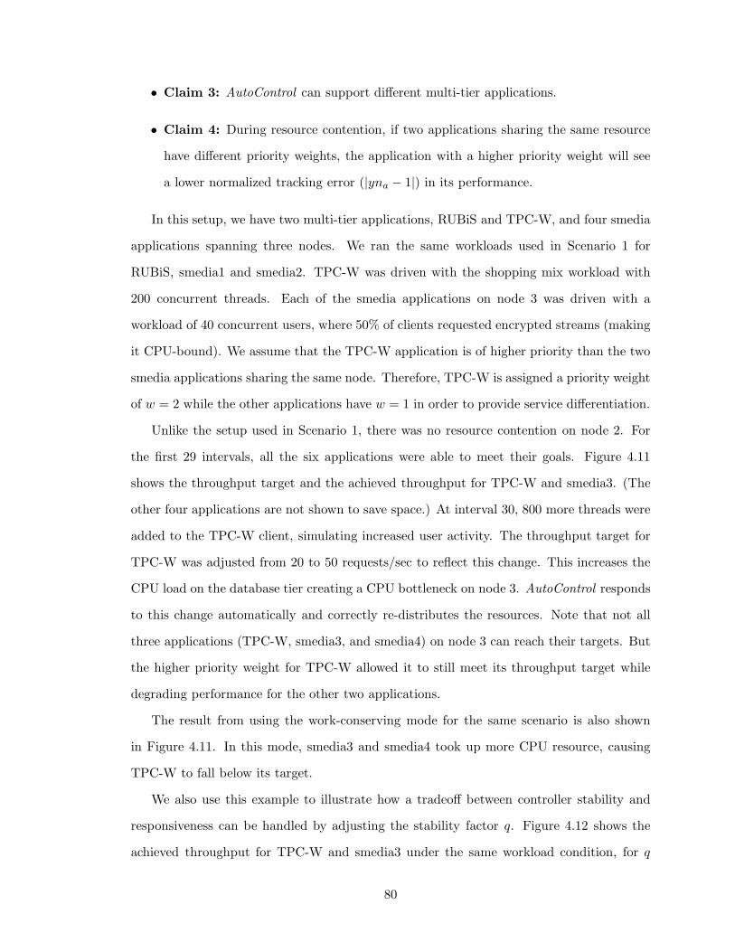
• Claim 3: AutoControl can support different multi-tier applications.
• Claim 4: During resource contention, if two applications sharing the same resource
have different priority weights, the application with a higher priority weight will see
a lower normalized tracking error (|yna − 1|) in its performance.
In this setup, we have two multi-tier applications, RUBiS and TPC-W, and four smedia
applications spanning three nodes. We ran the same workloads used in Scenario 1 for
RUBiS, smedia1 and smedia2. TPC-W was driven with the shopping mix workload with
200 concurrent threads. Each of the smedia applications on node 3 was driven with a
workload of 40 concurrent users, where 50% of clients requested encrypted streams (making
it CPU-bound). We assume that the TPC-W application is of higher priority than the two
smedia applications sharing the same node. Therefore, TPC-W is assigned a priority weight
of w = 2 while the other applications have w = 1 in order to provide service differentiation.
Unlike the setup used in Scenario 1, there was no resource contention on node 2. For
the first 29 intervals, all the six applications were able to meet their goals. Figure 4.11
shows the throughput target and the achieved throughput for TPC-W and smedia3. (The
other four applications are not shown to save space.) At interval 30, 800 more threads were
added to the TPC-W client, simulating increased user activity. The throughput target for
TPC-W was adjusted from 20 to 50 requests/sec to reflect this change. This increases the
CPU load on the database tier creating a CPU bottleneck on node 3. AutoControl responds
to this change automatically and correctly re-distributes the resources. Note that not all
three applications (TPC-W, smedia3, and smedia4) on node 3 can reach their targets. But
the higher priority weight for TPC-W allowed it to still meet its throughput target while
degrading performance for the other two applications.
The result from using the work-conserving mode for the same scenario is also shown
in Figure 4.11. In this mode, smedia3 and smedia4 took up more CPU resource, causing
TPC-W to fall below its target.
We also use this example to illustrate how a tradeoff between controller stability and
responsiveness can be handled by adjusting the stability factor q. Figure 4.12 shows the
achieved throughput for TPC-W and smedia3 under the same workload condition, for q
80
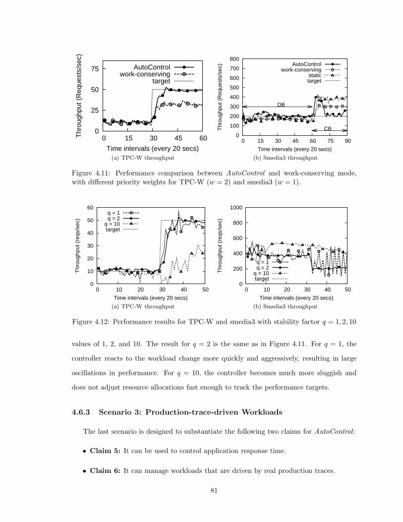
0
25
50
75
0 15 30 45 60Thr
ough
put (
Req
uest
s/se
c)
Time intervals (every 20 secs)
AutoControlwork-conserving
target
(a) TPC-W throughput
0
100
200
300
400
500
600
700
800
0 15 30 45 60 75 90
Thr
ough
put (
Req
uest
s/se
c)
Time intervals (every 20 secs)
DB
CB
AutoControlwork-conserving
statictarget
(b) Smedia3 throughput
Figure 4.11: Performance comparison between AutoControl and work-conserving mode,with different priority weights for TPC-W (w = 2) and smedia3 (w = 1).
0
10
20
30
40
50
60
0 10 20 30 40 50
Thr
ough
put (
reqs
/sec
)
Time intervals (every 20 secs)
q = 1q = 2
q = 10target
(a) TPC-W throughput
0
200
400
600
800
1000
0 10 20 30 40 50
Thr
ough
put (
reqs
/sec
)
Time intervals (every 20 secs)
q = 1q = 2
q = 10target
(b) Smedia3 throughput
Figure 4.12: Performance results for TPC-W and smedia3 with stability factor q = 1, 2, 10
values of 1, 2, and 10. The result for q = 2 is the same as in Figure 4.11. For q = 1, the
controller reacts to the workload change more quickly and aggressively, resulting in large
oscillations in performance. For q = 10, the controller becomes much more sluggish and
does not adjust resource allocations fast enough to track the performance targets.
4.6.3 Scenario 3: Production-trace-driven Workloads
The last scenario is designed to substantiate the following two claims for AutoControl :
• Claim 5: It can be used to control application response time.
• Claim 6: It can manage workloads that are driven by real production traces.
81

0 1 2 3 4 5 6 7 8
0 10 20 30 40 50 60 70 80
Res
pons
e tim
e (in
sec
s)
Time intervals (every 20 secs)
RUBiSsmedia1smedia2
target
(a) AutoControl
0 1 2 3 4 5 6 7 8
0 10 20 30 40 50 60 70 80
Res
pons
e tim
e (in
sec
s)
Time intervals (every 20 secs)
RUBiSsmedia1smedia2
target
(b) Work-conserving mode
0 1 2 3 4 5 6 7 8
0 10 20 30 40 50 60 70 80
Res
pons
e tim
e (in
sec
s)
Time intervals (every 20 secs)
RUBiSsmedia1smedia2
target
(c) Static allocation mode
Figure 4.13: Performance comparison of AutoControl, work-conserving mode and staticallocation mode, while running RUBiS, smedia1 and smedia2 with production-trace-drivenworkloads.
In this scenario, we use the same setup as in Scenario 1, shown in Figure 4.7(a). We
simulated the production workloads using the trace-driven approach as described in Sec-
tion 4.5. Each of the RUBiS, smedia1 and smedia2 applications was driven by a production
trace, while both smedia3 and smedia4 run a workload with 40 threads with a 2% chance
of requesting an encrypted stream (making it disk-bound).
In this experiment, we use response time as the performance metric for two reasons.
1. Response time behaves quite nonlinearly with respect to the resource allocation and
can be used to evaluate how AutoControl copes with nonlinearity in the system.
2. It is possible to specify the same response time target for all applications even if they
are different, whereas specifying throughput targets are harder since they may depend
82

on the offered load.
For brevity, we only show the results for the three applications running on node 1.
Figures 4.13a, 4.13b and 4.13c show the measured average response time of RUBiS, smedia1
and smedia2 as functions of the control interval, using AutoControl, work-conserving mode,
and static allocation mode, respectively. We use a response time target of 1.5 second for all
the three applications, and set the CPU allocation at a fixed 33% for each application in
the static mode. The dark-shaded regions show the time intervals when a CPU bottleneck
occurred.
In the first region, for the work-conserving mode, both smedia1 and smedia2 had high
CPU demands, causing not only response time target violations for themselves, but also a
large spike of 6 second in the response time for RUBiS at the 15th interval. In comparison,
AutoControl allocated to both smedia1 and smedia2 higher shares of the CPU without overly
penalizing RUBiS. As a result, all the three applications were able to meet the response
time target most of the time, except for the small spike in RUBiS.
In the second shaded region, the RUBiS application became more CPU intensive. Be-
cause there is no performance assurance in the work-conserving mode, the response time of
RUBiS surged and resulted in a period of target violations, while both smedia1 and smedia2
had response times well below the target. In contrast, AutoControl allocated more CPU
capacity to RUBiS when needed by carefully reducing the resource allocation to smedia2.
The result was that there were almost no target violations for any of the three applications.
The performance result from the static allocation mode was similar to that from the
work-conserving mode, except that the RUBiS response time was even worse in the second
region.
Despite the fact that response time is a nonlinear function of resource allocation, and
that the real traces used here were much more dynamic than the static workloads with step
changes tested in Scenario 1 and 2, AutoControl was still able to balance the resources and
minimize the response time violations for all three applications.
83
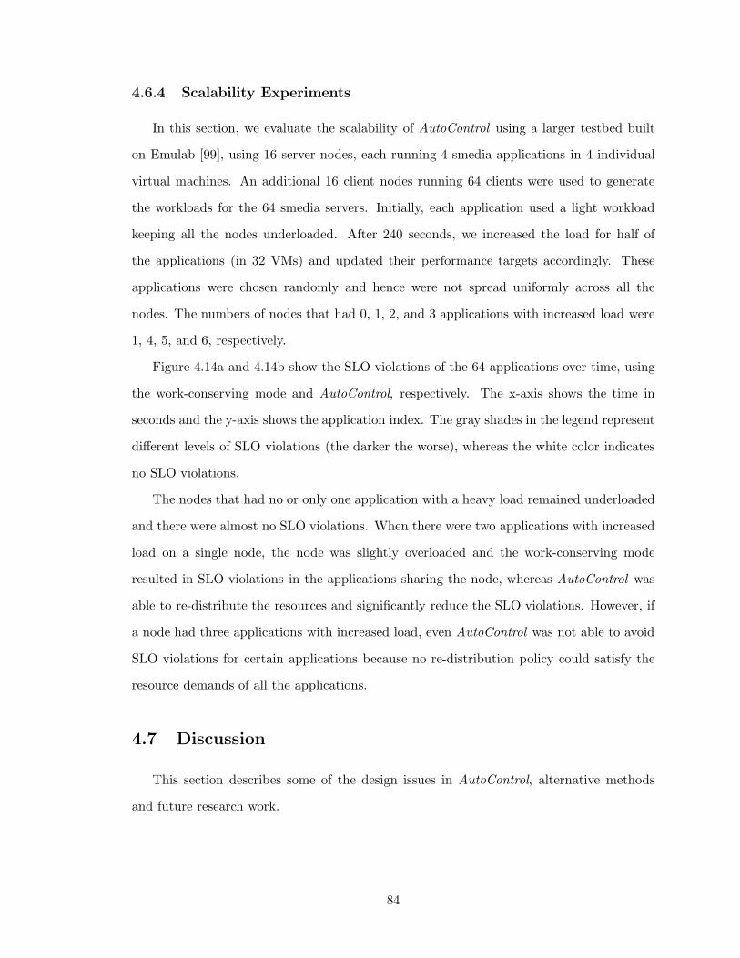
4.6.4 Scalability Experiments
In this section, we evaluate the scalability of AutoControl using a larger testbed built
on Emulab [99], using 16 server nodes, each running 4 smedia applications in 4 individual
virtual machines. An additional 16 client nodes running 64 clients were used to generate
the workloads for the 64 smedia servers. Initially, each application used a light workload
keeping all the nodes underloaded. After 240 seconds, we increased the load for half of
the applications (in 32 VMs) and updated their performance targets accordingly. These
applications were chosen randomly and hence were not spread uniformly across all the
nodes. The numbers of nodes that had 0, 1, 2, and 3 applications with increased load were
1, 4, 5, and 6, respectively.
Figure 4.14a and 4.14b show the SLO violations of the 64 applications over time, using
the work-conserving mode and AutoControl, respectively. The x-axis shows the time in
seconds and the y-axis shows the application index. The gray shades in the legend represent
different levels of SLO violations (the darker the worse), whereas the white color indicates
no SLO violations.
The nodes that had no or only one application with a heavy load remained underloaded
and there were almost no SLO violations. When there were two applications with increased
load on a single node, the node was slightly overloaded and the work-conserving mode
resulted in SLO violations in the applications sharing the node, whereas AutoControl was
able to re-distribute the resources and significantly reduce the SLO violations. However, if
a node had three applications with increased load, even AutoControl was not able to avoid
SLO violations for certain applications because no re-distribution policy could satisfy the
resource demands of all the applications.
4.7 Discussion
This section describes some of the design issues in AutoControl, alternative methods
and future research work.
84
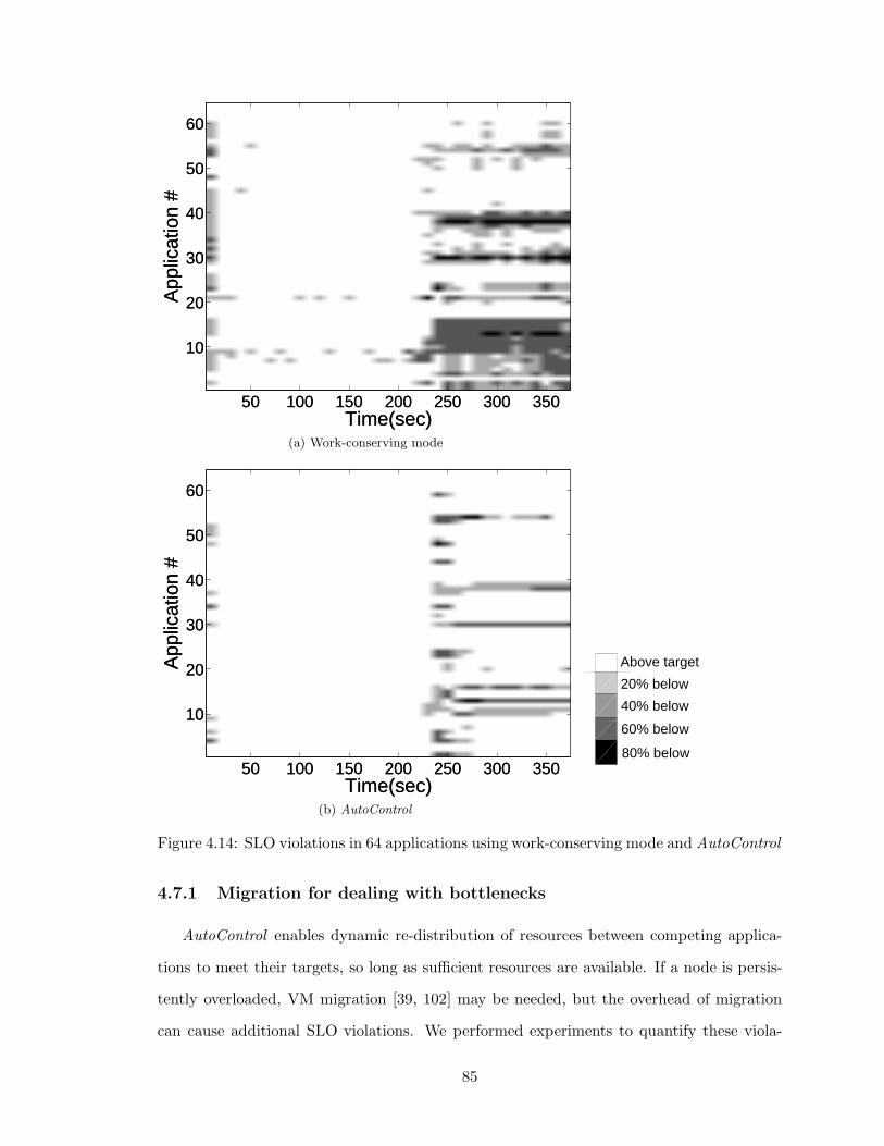
Time(sec)
App
licat
ion
#
50 100 150 200 250 300 350
10
20
30
40
50
60
Time(sec)
App
licat
ion
#
50 100 150 200 250 300 350
10
20
30
40
50
60
(a) Work-conserving mode
Time(sec)
App
licat
ion
#
50 100 150 200 250 300 350
10
20
30
40
50
60
Time(sec)
App
licat
ion
#
50 100 150 200 250 300 350
10
20
30
40
50
60
(b) AutoControl
20% below
Above target
40% below
60% below
80% below
Figure 4.14: SLO violations in 64 applications using work-conserving mode and AutoControl
4.7.1 Migration for dealing with bottlenecks
AutoControl enables dynamic re-distribution of resources between competing applica-
tions to meet their targets, so long as sufficient resources are available. If a node is persis-
tently overloaded, VM migration [39, 102] may be needed, but the overhead of migration
can cause additional SLO violations. We performed experiments to quantify these viola-
85
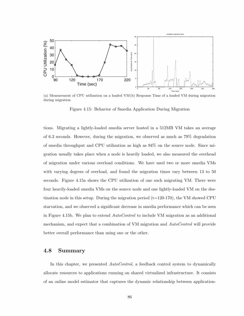
0
10
20
30
40
50
90 120 170 220
CP
U U
tiliz
atio
n (%
)
Time (sec)
(a) Measurement of CPU utilization on a loaded VMduring migration
0
5
10
15
20
25
30
0 40 80 120 160 200 240 280
Avg
Res
pons
e T
ime
(sec
)
Time (sec)
smedia4 response time
(b) Response Time of a loaded VM during migration
Figure 4.15: Behavior of Smedia Application During Migration
tions. Migrating a lightly-loaded smedia server hosted in a 512MB VM takes an average
of 6.3 seconds. However, during the migration, we observed as much as 79% degradation
of smedia throughput and CPU utilization as high as 94% on the source node. Since mi-
gration usually takes place when a node is heavily loaded, we also measured the overhead
of migration under various overload conditions. We have used two or more smedia VMs
with varying degrees of overload, and found the migration times vary between 13 to 50
seconds. Figure 4.15a shows the CPU utilization of one such migrating VM. There were
four heavily-loaded smedia VMs on the source node and one lightly-loaded VM on the des-
tination node in this setup. During the migration period (t=120-170), the VM showed CPU
starvation, and we observed a significant decrease in smedia performance which can be seen
in Figure 4.15b. We plan to extend AutoControl to include VM migration as an additional
mechanism, and expect that a combination of VM migration and AutoControl will provide
better overall performance than using one or the other.
4.8 Summary
In this chapter, we presented AutoControl, a feedback control system to dynamically
allocate resources to applications running on shared virtualized infrastructure. It consists
of an online model estimator that captures the dynamic relationship between application-
86
level performance and resource allocations and a MIMO resource controller that determines
appropriate allocations of multiple resources to achieve application-level SLOs.
We evaluated AutoControl using two testbeds consisting of varying numbers of Xen vir-
tual machines and various single- and multi- tier applications and benchmarks. Our experi-
mental results confirmed that AutoControl can detect dynamically-changing CPU and disk
bottlenecks across multiple nodes and can adjust resource allocations accordingly to achieve
end-to-end application-level SLOs. In addition, AutoControl can cope with dynamically-
shifting resource bottlenecks and provide a level of service differentiation according to the
priorities of individual applications. Finally, we showed that AutoControl can enforce per-
formance targets for different application-level metrics, including throughput and response
time, under dynamically-varying resource demands.
87
CHAPTER 5
Automated Control of Shared Storage Resources
5.1 Introduction
The common mode of running applications in corporate environments is to consolidate
them onto shared hardware in large data centers. This allows benefits such as improved
utilization of the resources, higher performance, and centralized management. However, as
more applications compete for shared resources, the system has to be flexible enough to
enable each application to meet its performance requirements.
Applications running on the shared storage present very different storage loads and have
different performance requirements: for example, Online Transaction Processing (OLTP)
applications might present bursty loads and require bounded IO response time; business
analytics may require high throughput; and back-up applications usually present intense,
highly sequential workloads with high throughput requirements. When the requirements of
all applications cannot be met, the choice of which application requirements to meet and
which ones to abandon may depend upon the priority of the individual applications. For
example, meeting the I/O response time requirement of an interactive system may take
precedence over the throughput requirement of a backup system. A data center operator
needs the flexibility to set the performance metrics and priority levels for the applications,
and to adjust them as necessary.
The proposed solutions to this problem in the literature include using proportional share
I/O schedulers (e.g., SFQ [55]) and admission control (I/O throttling) using feedback con-
88
trollers (e.g., Triage [60]). Proportional share schedulers divide the throughput available
from the storage device between the applications in proportion to the applications’ shares
(a.k.a. weights), which are set statically by an administrator. Such schedulers alone can-
not provide application performance differentiation, for several reasons: 1) the application
performance depends on the proportional share settings and the workload characteristics
in a complex, non-linear, time-dependent manner, and it is difficult for an administrator to
determine in advance the share to assign to each application, and how/when to change it;
2) applications have several kinds of performance targets, such as response time and band-
width requirements, not just throughput; and 3) in overload situations, when the system is
unable to meet all of the application QoS requirements, prioritization is necessary to enable
important applications to meet their performance requirements.
In this chapter, we present an approach that combines an optimization-based feedback
controller with an underlying IO scheduler. Our controller accepts performance metrics
and targets from multiple applications, monitors the performance of each application, and
periodically adjusts the IO resources given to the applications at the disk array to make
sure that each application meets its performance goal. The performance metrics for the
applications can be different: the controller normalizes the application metrics so that
the performance received by different applications can be compared and traded off. Our
controller continually models the performance of each application relative to the resources
it receives, and uses this model to determine the appropriate resource allocation for the
application. If the resources available are inadequate to provide all the applications with
their desired performance, a Linear Programming optimizer is used to compute a resource
allocation that will degrade each application’s performance in inverse proportion to its
priority. Initial evaluations using this controller with a large commercial disk array show
very promising results.
5.2 Storage Controller Design
In this section, we first describe our system model. We then present our design of the
storage controller and describe its components in detail.
89
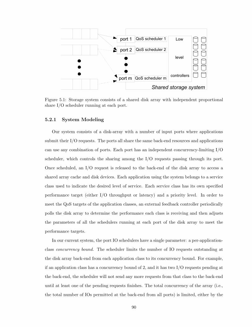
Figure 5.1: Storage system consists of a shared disk array with independent proportionalshare I/O scheduler running at each port.
5.2.1 System Modeling
Our system consists of a disk-array with a number of input ports where applications
submit their I/O requests. The ports all share the same back-end resources and applications
can use any combination of ports. Each port has an independent concurrency-limiting I/O
scheduler, which controls the sharing among the I/O requests passing through its port.
Once scheduled, an I/O request is released to the back-end of the disk array to access a
shared array cache and disk devices. Each application using the system belongs to a service
class used to indicate the desired level of service. Each service class has its own specified
performance target (either I/O throughput or latency) and a priority level. In order to
meet the QoS targets of the application classes, an external feedback controller periodically
polls the disk array to determine the performance each class is receiving and then adjusts
the parameters of all the schedulers running at each port of the disk array to meet the
performance targets.
In our current system, the port IO schedulers have a single parameter: a per-application-
class concurrency bound. The scheduler limits the number of IO requests outstanding at
the disk array back-end from each application class to its concurrency bound. For example,
if an application class has a concurrency bound of 2, and it has two I/O requests pending at
the back-end, the scheduler will not send any more requests from that class to the back-end
until at least one of the pending requests finishes. The total concurrency of the array (i.e.,
the total number of IOs permitted at the back-end from all ports) is limited, either by the
90
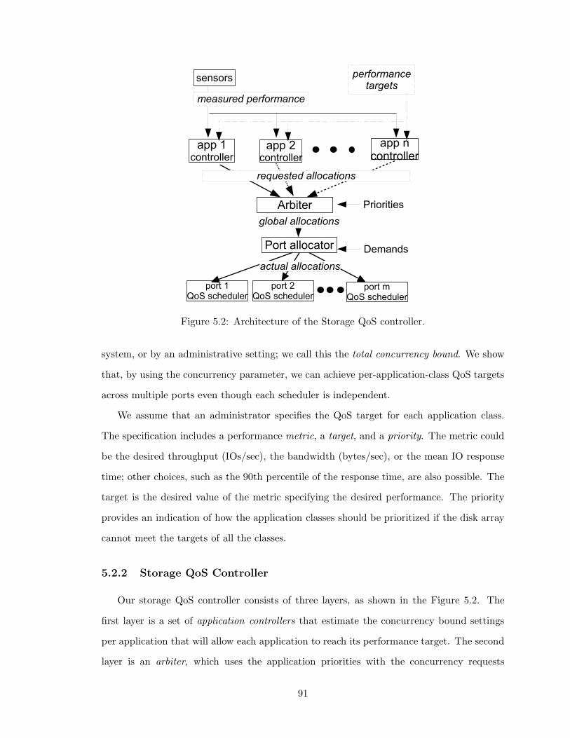
Figure 5.2: Architecture of the Storage QoS controller.
system, or by an administrative setting; we call this the total concurrency bound. We show
that, by using the concurrency parameter, we can achieve per-application-class QoS targets
across multiple ports even though each scheduler is independent.
We assume that an administrator specifies the QoS target for each application class.
The specification includes a performance metric, a target, and a priority. The metric could
be the desired throughput (IOs/sec), the bandwidth (bytes/sec), or the mean IO response
time; other choices, such as the 90th percentile of the response time, are also possible. The
target is the desired value of the metric specifying the desired performance. The priority
provides an indication of how the application classes should be prioritized if the disk array
cannot meet the targets of all the classes.
5.2.2 Storage QoS Controller
Our storage QoS controller consists of three layers, as shown in the Figure 5.2. The
first layer is a set of application controllers that estimate the concurrency bound settings
per application that will allow each application to reach its performance target. The second
layer is an arbiter, which uses the application priorities with the concurrency requests
91
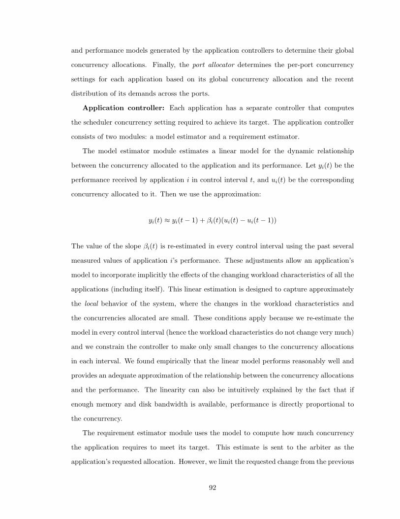
and performance models generated by the application controllers to determine their global
concurrency allocations. Finally, the port allocator determines the per-port concurrency
settings for each application based on its global concurrency allocation and the recent
distribution of its demands across the ports.
Application controller: Each application has a separate controller that computes
the scheduler concurrency setting required to achieve its target. The application controller
consists of two modules: a model estimator and a requirement estimator.
The model estimator module estimates a linear model for the dynamic relationship
between the concurrency allocated to the application and its performance. Let yi(t) be the
performance received by application i in control interval t, and ui(t) be the corresponding
concurrency allocated to it. Then we use the approximation:
yi(t) ≈ yi(t− 1) + βi(t)(ui(t)− ui(t− 1))
The value of the slope βi(t) is re-estimated in every control interval using the past several
measured values of application i’s performance. These adjustments allow an application’s
model to incorporate implicitly the effects of the changing workload characteristics of all the
applications (including itself). This linear estimation is designed to capture approximately
the local behavior of the system, where the changes in the workload characteristics and
the concurrencies allocated are small. These conditions apply because we re-estimate the
model in every control interval (hence the workload characteristics do not change very much)
and we constrain the controller to make only small changes to the concurrency allocations
in each interval. We found empirically that the linear model performs reasonably well and
provides an adequate approximation of the relationship between the concurrency allocations
and the performance. The linearity can also be intuitively explained by the fact that if
enough memory and disk bandwidth is available, performance is directly proportional to
the concurrency.
The requirement estimator module uses the model to compute how much concurrency
the application requires to meet its target. This estimate is sent to the arbiter as the
application’s requested allocation. However, we limit the requested change from the previous
92
allocation (by 5% of the total concurrency bound in our current implementation) to ensure
that the system remains in a local operating region where the estimated linear model still
applies. Also, the data from which the model is estimated is often noisy, and the resulting
models can occasionally be quite inaccurate. Limiting the change in concurrency within a
control cycle also limits the harm caused by an inaccurate model. The cost of this limit is
that convergence to a new operating point is slowed down when application characteristics
change, but we found rate of convergence adequate in empirical tests.
Arbiter: The arbiter computes the applications’ actual global concurrency settings
based on their priorities. In each control cycle, the arbiter receives the concurrency re-
quests and the models used to derive them from each of the application controllers. There
are two cases, the underload case, where the total concurrency bound is large enough to
meet the independent requests submitted by the application controllers, and the overload
case, where the total concurrency bound is smaller than the sum of the requests. In the
case of underload, the scheduler parameters are set based on the application controllers’ re-
quests, and any excess concurrency available is distributed in proportion to the application
priorities. In the overload case, the arbiter uses a linear optimization to find concurrency
settings that will degrade each application’s performance (relative to its target) in inverse
proportion to its priority, as far as possible. As in the application controllers, we limit the
deviation from the previous allocations so that the estimated linear model is applicable.
More precisely, say that there are n applications, pi is the priority of application i, ci its
current allocation, ui the next (future) allocation, and fi is the linear model estimating the
performance of application i in terms of ui. li is the limit on deviation, which we set to 0.05
for all applications. The concurrency allocations ci and ui are normalized to the range [0, 1]
by dividing the actual allocation by the total concurrency bound. The performance values
fi(ui) are normalized to be (performance/target) for throughput and bandwidth metrics
and (target/performance) for latency, in order to make all normalized performance values
better as they increase. In order to compute the future allocations ui, the arbiter solves the
93
following linear program:
Find u1, . . . , un, ǫ to minimize ǫ subject to:
pi(1− fi(ui))−pj(1− fj(uj)) < ǫ
for 1 ≤ i 6= j ≤ n
|ui − ci| ≤ li for 1 ≤ i ≤ n
u1 + · · ·+ un = min(1, c1 + l1 + · · ·+ cn + ln).
Note that the quantity in the right-hand side of the last constraint is a constant for the
linear program, and the constraint is therefore still linear.
In the LP above, pi(1−fi(ui)) is the fractional tracking error for application i, weighted
by its priority. ǫ is the maximum difference between the priority-weighted fractional tracking
errors for different applications, and the objective function tries to minimize this maximum
difference. In the limit, ǫ = 0, and the priority-weighted fractional tracking errors are equal;
for example, in a scenario with two applications, if application 1 has the priority 1 and a
performance value 10% below its target, and application 2 has the priority 2, then each has
a priority-weighted tracking error of 0.1, and the performance value of application 2 should
be 5% below its target.
Port allocator: The arbiter computes the aggregate concurrency setting for each ap-
plication, but this concurrency has to be translated into per-port settings. Since application
workloads may be dynamic and non-uniform across the ports, the port allocator uses the
recently observed demand from each application at the ports to determine how much of the
application’s concurrency should be allocated to a port. We define an application’s demand
at a port as the mean number of IO requests outstanding from the application at the port
during the previous control interval.
More precisely, let di,j denote the the demand of application i through port j, and CGi
its aggregate concurrency as determined by the arbiter. Then the corresponding per-port
94

normalized concurrencies are given by:
Ci,j = CGi
(
di,j∑n
k=1 di,k
)
where n is the number of ports. If di,j is zero, then the corresponding concurrency is set to
zero.
The normalized concurrencies are multiplied by the total concurrency bound and rounded
up to determine the number of application IOs permitted to be scheduled simultaneously
from that port. In addition, we set the concurrency setting to be at least one for all appli-
cations at all ports, in order to avoid blocking an application that begins sending IOs to a
port during the control interval.
5.3 Evaluation Results
In this section, we present our initial results from a set of experiments we conducted
to evaluate our storage controller. We designed our experiments to determine whether
our controller can adjust the low-level scheduler parameters to achieve application targets.
We also evaluated its ability to differentiate between multiple applications based on their
priorities. Finally, we looked at the behavior of our controller when applications have
different target metrics, for example a latency target and a throughput target.
We used two HP BL460c blade servers and a high-end XP-1024 disk array for our
experiments. The blade servers are connected to separate ports of the XP-1024 disk array
via two 4 Gbit/s QLogic Fibre channel adapters. Each of the blade servers had 8GB RAM,
two 3GHz dual core Intel Xeon processors and used the Linux kernel version 2.6.18-8.el5 as
their operating system. We allocated seven 4-disk RAID-1 logical disks for our experiments
on the XP disk array.
Since the XP array did not have an appropriate port scheduler that can limit available
concurrency to specific workloads, we implemented a scheduler in the Linux kernel and ran
it at each of the hosts to emulate independent port schedulers. The scheduler module creates
pseudo devices (entries in /dev), which are then backed up by the logical disks at the XP
95
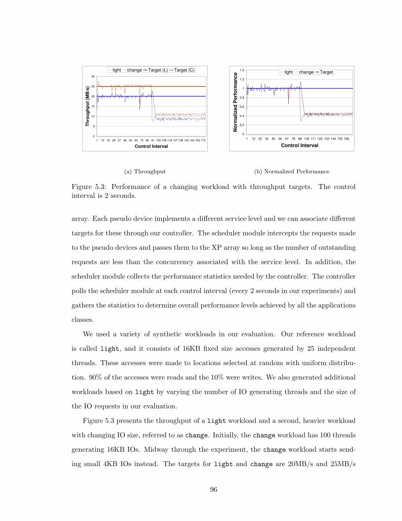
0
5
10
15
20
25
30
1 10 19 28 37 46 55 64 73 82 91 100 109 118 127 136 145 154 163 172
Control Interval
Th
rou
gh
pu
t (M
B/s
)
light change Target (L) Target (C)
(a) Throughput
0
0.2
0.4
0.6
0.8
1
1.2
1.4
1 12 23 34 45 56 67 78 89 100 111 122 133 144 155 166
Control Interval
No
rma
lize
d P
erf
orm
an
ce light change Target
(b) Normalized Performance
Figure 5.3: Performance of a changing workload with throughput targets. The controlinterval is 2 seconds.
array. Each pseudo device implements a different service level and we can associate different
targets for these through our controller. The scheduler module intercepts the requests made
to the pseudo devices and passes them to the XP array so long as the number of outstanding
requests are less than the concurrency associated with the service level. In addition, the
scheduler module collects the performance statistics needed by the controller. The controller
polls the scheduler module at each control interval (every 2 seconds in our experiments) and
gathers the statistics to determine overall performance levels achieved by all the applications
classes.
We used a variety of synthetic workloads in our evaluation. Our reference workload
is called light, and it consists of 16KB fixed size accesses generated by 25 independent
threads. These accesses were made to locations selected at random with uniform distribu-
tion. 90% of the accesses were reads and the 10% were writes. We also generated additional
workloads based on light by varying the number of IO generating threads and the size of
the IO requests in our evaluation.
Figure 5.3 presents the throughput of a light workload and a second, heavier workload
with changing IO size, referred to as change. Initially, the change workload has 100 threads
generating 16KB IOs. Midway through the experiment, the change workload starts send-
ing small 4KB IOs instead. The targets for light and change are 20MB/s and 25MB/s
96
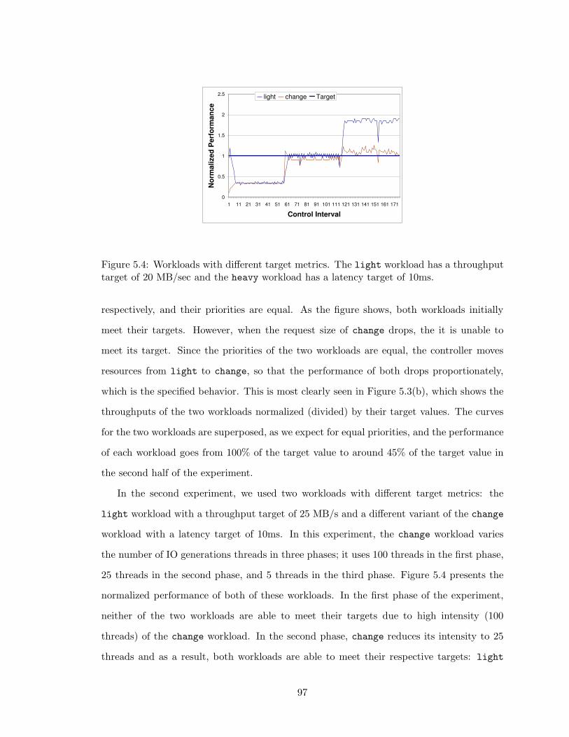
0
0.5
1
1.5
2
2.5
1 11 21 31 41 51 61 71 81 91 101 111 121 131 141 151 161 171
Control IntervalN
orm
ali
ze
d P
erf
orm
an
ce
light change Target
Figure 5.4: Workloads with different target metrics. The light workload has a throughputtarget of 20 MB/sec and the heavy workload has a latency target of 10ms.
respectively, and their priorities are equal. As the figure shows, both workloads initially
meet their targets. However, when the request size of change drops, the it is unable to
meet its target. Since the priorities of the two workloads are equal, the controller moves
resources from light to change, so that the performance of both drops proportionately,
which is the specified behavior. This is most clearly seen in Figure 5.3(b), which shows the
throughputs of the two workloads normalized (divided) by their target values. The curves
for the two workloads are superposed, as we expect for equal priorities, and the performance
of each workload goes from 100% of the target value to around 45% of the target value in
the second half of the experiment.
In the second experiment, we used two workloads with different target metrics: the
light workload with a throughput target of 25 MB/s and a different variant of the change
workload with a latency target of 10ms. In this experiment, the change workload varies
the number of IO generations threads in three phases; it uses 100 threads in the first phase,
25 threads in the second phase, and 5 threads in the third phase. Figure 5.4 presents the
normalized performance of both of these workloads. In the first phase of the experiment,
neither of the two workloads are able to meet their targets due to high intensity (100
threads) of the change workload. In the second phase, change reduces its intensity to 25
threads and as a result, both workloads are able to meet their respective targets: light
97
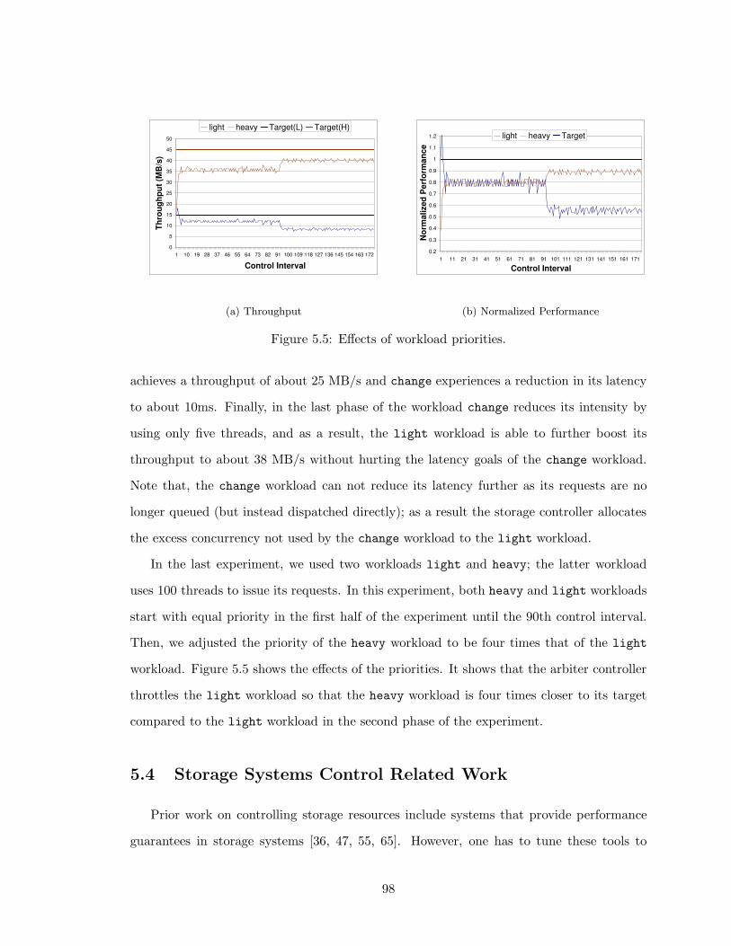
0
5
10
15
20
25
30
35
40
45
50
1 10 19 28 37 46 55 64 73 82 91 100 109 118 127 136 145 154 163 172
Control Interval
Th
rou
gh
pu
t (M
B/s
)
light heavy Target(L) Target(H)
(a) Throughput
0.2
0.3
0.4
0.5
0.6
0.7
0.8
0.9
1
1.1
1.2
1 11 21 31 41 51 61 71 81 91 101 111 121 131 141 151 161 171
Control Interval
No
rma
lize
d P
erf
orm
an
ce
light heavy Target
(b) Normalized Performance
Figure 5.5: Effects of workload priorities.
achieves a throughput of about 25 MB/s and change experiences a reduction in its latency
to about 10ms. Finally, in the last phase of the workload change reduces its intensity by
using only five threads, and as a result, the light workload is able to further boost its
throughput to about 38 MB/s without hurting the latency goals of the change workload.
Note that, the change workload can not reduce its latency further as its requests are no
longer queued (but instead dispatched directly); as a result the storage controller allocates
the excess concurrency not used by the change workload to the light workload.
In the last experiment, we used two workloads light and heavy; the latter workload
uses 100 threads to issue its requests. In this experiment, both heavy and light workloads
start with equal priority in the first half of the experiment until the 90th control interval.
Then, we adjusted the priority of the heavy workload to be four times that of the light
workload. Figure 5.5 shows the effects of the priorities. It shows that the arbiter controller
throttles the light workload so that the heavy workload is four times closer to its target
compared to the light workload in the second phase of the experiment.
5.4 Storage Systems Control Related Work
Prior work on controlling storage resources include systems that provide performance
guarantees in storage systems [36, 47, 55, 65]. However, one has to tune these tools to
98

achieve application-level guarantees. Our work builds on top of our earlier work, where we
developed an adaptive controller [60] to achieve performance differentiation, and efficient
adaptive proportional share scheduler [48] for storage systems.
In prior work, feedback controllers have been proposed [36, 60] to implement application
prioritization requirements by using client throttling. A centralized controller monitors the
state of the storage device and the application clients, and then directs the clients to reduce
or increase their IO request rate so that the requirements of the highest priority (or most
demanding) client can be met. This approach can handle somewhat more complex priori-
tization requirements than a simple proportional share scheduler, but has the disadvantage
that, by the time the clients implement the throttle commands, the state of the storage
device may have changed; as a result, the controller may not be work-conserving, and the
utilization of the storage device may be kept unnecessarily low.
In recent years, control theory has been applied to computer systems for resource man-
agement and performance control [52, 58]. Examples of its application include web server
performance guarantees [22], dynamic adjustment of the cache size for multiple request
classes [64], CPU and memory utilization control in web servers [43], adjustment of re-
source demands of virtual machines based on resource availability [103], and dynamic CPU
allocations for multi-tier applications [63, 76]. In our prior work [75], we have developed
a MIMO controller that can adjust the resource shares for multiple virtual machines to
achieve application targets. In contrast, this work focuses on building a control system for
a shared disk array with multiple ports. We also introduce the notion of resource control
using dynamic concurrency bounds to provide performance differentiation across multiple
ports.
5.5 Summary
In this chapter, we presented a storage controller that dynamically allocates storage
resources to multiple competing applications accessing data on a multi-port shared disk
array. The controller consists of three layers, a set of application controllers, an arbiter
and a port allocator. The application controllers determine the required I/O resources to
99
meet application performance goals, and the arbiter uses application priorities to arbitrate
in the case of overload. The port allocator uses each application’s demands through a
particular port to determine the per-port concurrency. Our preliminary experiments show
that our controller can achieve application targets by automatically adjusting the scheduler
parameters. The controller can also enforce different application priorities and different
targets for multiple applications.
100
CHAPTER 6
Automated Mechanisms for Saving Desktop Energy using
Virtualization
6.1 Introduction
The energy consumed by the burgeoning computing infrastructure worldwide has re-
cently drawn significant attention. While the focus of energy management has been on
the data-center setting [37, 69, 73], attention has also been directed recently to the signifi-
cant amounts of energy consumed by desktop computers in homes and enterprises [23, 71].
A recent study [74] estimates that PCs and their monitors consume about 100 TWh/year,
constituting 3% of the annual electricity consumed in the U.S. Of this, 65 TWh/year is con-
sumed by PCs in enterprises, which constitutes 5% of the commercial building electricity
consumption.
The common approach to reducing PC energy wastage is to put a computer to sleep
or turn it off when it is idle. However, the presence of the user makes this particularly
challenging in a desktop computing environment. Users care about preserving long-running
network connections (e.g., login sessions, IM presence, file sharing), background computa-
tion (e.g., syncing and automatic filing of new emails), and keeping their machine reachable
even while it is idle. Putting a desktop PC to sleep is likely to cause disruption (e.g., bro-
ken connections), thereby having a negative impact on the user, who might then choose to
disable the energy savings mechanism altogether.
To reduce user disruption while still allowing machines to sleep, the typical approach
101

has been to have a proxy on the network for a machine that is asleep [74]. However, this
approach suffers from an inherent tradeoff between functionality and complexity in terms
of application-specific customization.
In this chapter, we present LiteGreen, a system to save desktop energy by employing a
novel approach to avoiding user disruption as well as the complexity of application-specific
customization. The basic idea is to virtualize the user’s desktop computing environment as a
virtual machine (VM) and then migrate it between the user’s physical desktop machine and
a VM server, depending on whether the desktop computing environment is being actively
used or is idle. When the desktop becomes idle, say when the user steps away for several
minutes (e.g., for a coffee break), the desktop VM is migrated away to the VM server and
the physical desktop machine is put to standby sleep mode. When the desktop becomes
active again (e.g., when the user returns), the desktop VM is migrated back to the physical
desktop machine. Thus, even when it has been migrated to the VM server, the user’s desktop
environment remains alive (i.e., it is “always on”), so ongoing network connections and
other activities (e.g., background downloads) are not disturbed, regardless of the application
involved. A fundamental assumption is LiteGreen is that the current systems are not energy
proportional.
The “always on” feature of LiteGreen allows energy savings whenever the opportunity
arises, without having to worry about disrupting the user. Besides long idle periods (e.g.,
nights and weekends), energy can also be saved by putting the physical desktop computer
to sleep even during short idle periods, such as when a user goes to a meeting or steps
out for coffee. Indeed, our measurements indicate that the potential energy savings from
exploiting short idle periods are significant (Section 6.3).
While virtualization is a useful primitive for continuously maintaining the desktop envi-
ronment, the following two key challenges need to be addressed for virtualization to be useful
for saving energy on desktop computers. First, how do we provide a normal (undisrupted)
desktop experience to users, masking the effect of VMs and their migration? Second, how
do we decide when and which VMs to migrate to/from the server in order to maximize
energy savings while minimizing disruption to users?
To address the first challenge, LiteGreen uses the live migration feature supported by
102
modern hypervisors [39] coupled with the idea of always presenting the desktop environment
through a level of indirection (Section 6.4). Thus, whether the VM is at the server or
desktop, users always access their desktop VM through a remote desktop (RD) session. So,
in a typical scenario, when a user returns to their machine that has been put to sleep, the
machine is woken up from sleep and the user is able to immediately access their desktop
environment (whose state is fully up-to-date, because it has been “always on”) through an
RD connection to the desktop VM running on the VM server. Subsequently, the desktop
VM is migrated back to the user’s physical desktop machine without the user even noticing.
To address the second challenge, LiteGreen uses an energy-saving algorithm that runs
on the server and carefully balances migrations based on two continuously-updated lists: 1)
VMs in mandatory to push list need to be migrated to the desktop to minimize user disrup-
tion and 2) VMs in eligible to pull list may be migrated to server for energy savings, subject
to server capacity constraints (Section 5.2). Based on an analysis of an aggregate of over
65,000 hours of data we have gathered from 120 desktop computers at Microsoft Research
India (MSRI), we estimate that LiteGreen saves 72-86% of desktop energy, compared to
35% savings achieved by either users manually or automatically putting their machines to
sleep through Windows power management.
We have prototyped LiteGreen on the Microsoft Hyper-V hypervisor (Section 6.7). We
have a small-scale deployment running on the desktop machines of five users. Separately,
we have conducted laboratory experiments using both the Hyper-V and Xen hypervisors to
evaluate various aspects of LiteGreen. A simulator is also developed to analyze the gathered
data and understand the finer aspects of our algorithms.
The main contributions of this work are the following:
1. A novel system that leverages virtualization to consolidate idle desktops on a VM
server, thereby saving energy while avoiding user disruption.
2. Automated mechanisms to drive the migration of the desktop computing environment
between the physical desktop machines and the VM server.
3. A prototype implementation and the evaluation of LiteGreen through a small-scale
deployment.
103

4. Trace-driven analysis based on an aggregate of over 65,000 hours of desktop resource
usage data gathered from 120 desktops, demonstrating total energy savings of 72-86%
with short idle periods (< 3 hours) contributing 20% or more.
6.2 Background
In this section, we provide some background on the problem setting and and discuss
related work.
6.2.1 PC Energy Consumption
Researchers have measured and characterized the energy consumed by desktop comput-
ers [23]. The typical desktop PC consumes 80-110 W when active and 60-80 W when idle,
excluding the monitor, which adds another 35-80 W. The relatively small difference between
active and idle modes is significant and arises because the processor itself only accounts for
a small portion of the total energy. So saving energy using the multiple P (“processor”)
states, effected through dynamic voltage and frequency scaling (DVFS) [97], has limited
effectiveness.
In view of the above, multiple S (“sleep”) states have been defined as part of the ACPI
standard [17]. In particular, the S3 state (“standby”) suspends the machine’s state to RAM,
thereby cutting energy consumption to 2-3 W. S3 has the advantage of being much quicker
to transition in and out of than S4 (“hibernate”), which involves suspending the machine’s
state to disk.
6.2.2 Proxy-Based Approach
As discussed above, the only way of cutting down the energy consumed by a PC is to put
it to sleep. However, when a PC it put to sleep, it loses its network presence, resulting in
ongoing connections breaking (e.g., remote login or file download sessions) and the machine
even becoming inaccessible over the network. The resulting disruption has been recognized
as a key reason why users are often reluctant to put their machines to sleep [23].
The general approach to allowing a PC to sleep while maintaining some network presence
104
is to have a network proxy operate on its behalf while it is asleep [74]. The functionality of
the proxy could span a wide range as follows.
• WoL Proxy: The simplest proxy allows the machine to be woken up using the Wake-
on-LAN (WoL) mechanism [16] supported by the vast majority of Ethernet NICs in
deployment. To be able to send the “magic” WoL packet, the proxy must be on the
same subnet as the target machine and, moreover, needs to know the MAC address
of the machine. Typically, machine wakeup is initiated manually.
• Protocol Proxy: A more sophisticated proxy performs automatic wakeup, triggered
by a filtered subset of the incoming traffic [71]. The filters could be configured based
on user input and also the list of network ports that the target machine was listening
on before it went to sleep. Other traffic is either responded to by the proxy itself
without waking up the target machine (e.g., ARP for the target machine) or ignored
(e.g., ARP for other hosts).
• Application Proxy: An even more sophisticated proxy incorporates application-
specific stubs that allow it to engage in network communication on behalf of appli-
cations running on the machine that is now asleep [71]. Such a proxy could even be
integrated into a NIC augmented with processing and storage [23].
The greater functionality of a proxy comes at the cost of greater complexity, for instance,
the need to create stubs for each application that the user wishes to keep alive. LiteGreen
sidesteps this complexity by keeping the entire desktop computing environment alive, by
consolidating it on the server along with other idle desktops.
6.2.3 Saving Energy through Consolidation
Consolidation to save energy has been employed in other computing settings—data
centers and thin clients.
In the data center setting, server consolidation is used to approximate energy propor-
tionality, wherein the overall energy consumption is roughly proportional to the workload.
Since the individual computing nodes are far from being energy-proportional, the approach
105
taken is to migrate computation, typically using virtualization, from several lightly-loaded
servers onto fewer servers and then turn off the servers that are freed up [37, 86, 90]. Do-
ing so saves not only the energy consumed directly by the servers but also the significant
amount of energy consumed indirectly for cooling. For instance, there has been work on
workload placement based on the spatial temperature profile within the data center [69]
and coordinated power management in such settings [70].
Thin client based computing, an idea that is making a reappearance [41, 15] despite
failures in the past, represents an extreme form of consolidation, with all of the computing
resources being centralized. While the cost, management, and energy savings might make
the model attractive in some environments, it may not be suitable in settings where power
users want the flexibility of a PC or insulation from even transient dips in performance
due to consolidation. Indeed, market projections suggest that PCs will continue to be the
dominant desktop computing platform, with over 125 million units shipping each year from
2009 through 2013 [21], and with thin clients replacing only 15% of PCs by 2014 [19]. Thus,
there will continue to be a sizeable and growing installed base of PCs for the foreseeable
future, so addressing the problem of energy consumed by desktop PCs remains important.
While LiteGreen’s use of consolidation is inspired by the above work, a key difference
arises from the presence of users in a desktop computing environment. Unlike in a data
center setting, where machines tend to run server workloads and hence substitutable to a
large extent, a desktop machine is a user’s personal computer. Users expect to have access
to their computing environment. Furthermore, unlike in a thin client setting, users expect
to have good interactive performance and the flexibility of attaching specialized hardware
and peripherals (e.g., a high-end graphics card).
Central to the design of LiteGreen is preserving this PC model and minimizing user
disruption by consolidating only idle desktops.
6.2.4 Virtualization in LiteGreen Prototype
For our LiteGreen prototype, we use the Microsoft Hyper-V hypervisor. While this is
a server hypervisor, the five users in our deployment were able to use it without difficulty
in their desktop computing environment. Since, Hyper-V currently does not support page
106
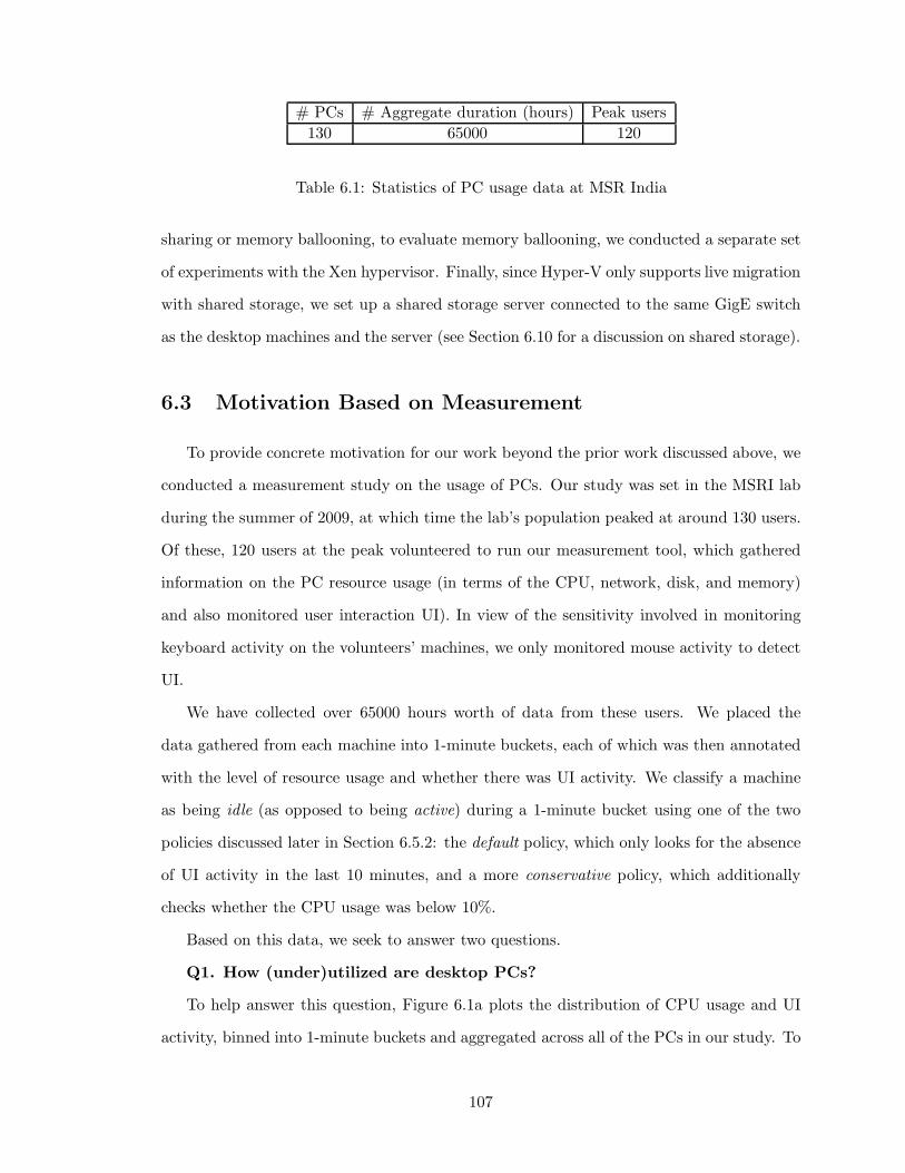
# PCs # Aggregate duration (hours) Peak users
130 65000 120
Table 6.1: Statistics of PC usage data at MSR India
sharing or memory ballooning, to evaluate memory ballooning, we conducted a separate set
of experiments with the Xen hypervisor. Finally, since Hyper-V only supports live migration
with shared storage, we set up a shared storage server connected to the same GigE switch
as the desktop machines and the server (see Section 6.10 for a discussion on shared storage).
6.3 Motivation Based on Measurement
To provide concrete motivation for our work beyond the prior work discussed above, we
conducted a measurement study on the usage of PCs. Our study was set in the MSRI lab
during the summer of 2009, at which time the lab’s population peaked at around 130 users.
Of these, 120 users at the peak volunteered to run our measurement tool, which gathered
information on the PC resource usage (in terms of the CPU, network, disk, and memory)
and also monitored user interaction UI). In view of the sensitivity involved in monitoring
keyboard activity on the volunteers’ machines, we only monitored mouse activity to detect
UI.
We have collected over 65000 hours worth of data from these users. We placed the
data gathered from each machine into 1-minute buckets, each of which was then annotated
with the level of resource usage and whether there was UI activity. We classify a machine
as being idle (as opposed to being active) during a 1-minute bucket using one of the two
policies discussed later in Section 6.5.2: the default policy, which only looks for the absence
of UI activity in the last 10 minutes, and a more conservative policy, which additionally
checks whether the CPU usage was below 10%.
Based on this data, we seek to answer two questions.
Q1. How (under)utilized are desktop PCs?
To help answer this question, Figure 6.1a plots the distribution of CPU usage and UI
activity, binned into 1-minute buckets and aggregated across all of the PCs in our study. To
107

0
10
20
30
40
50
60
70
80
90
100
0 10 20 30 40 50 60 70 80 90 100
CD
F
CPU utilization
CPU with UICPU only
(a) Distribution of CPU utilization
0
20
40
60
80
100
120
140
160
180
200
07/1323:0007/1323:00
07/1400:0007/1400:0007/1400:00
07/1401:0007/1401:00
07/1402:0007/1402:0007/1402:00
07/1403:0007/1403:00
07/1404:0007/1404:0007/1404:00
07/1405:0007/1405:00
07/1406:0007/1406:0007/1406:00
07/1407:0007/1407:00
07/1408:0007/1408:0007/1408:00
07/1409:0007/1409:00
07/1410:0007/1410:0007/1410:00
07/1411:0007/1411:00
07/1412:00
Net
wor
k th
roug
hput
(K
Byt
es/s
ec)
Time
(b) Network activity during the night on one idle desk-top machine
1
10
100
1000
0 10 20 30 40 50 60 70
Tot
al ti
me
(in h
ours
, log
scal
e)
Idle bins (hours)
DefaultConservative
(c) Distribution of idle periods
��������
��������
ConservativeDefault
��������
��������
��������������������������������
��������������������������������
������������������
������������������
����������
����������
0
15,000 20,000 25,000 30,000 35,000 40,000 45,000
<= 3 hrs > 3 hrs
Tot
al T
ime
(in h
ours
)
5,000 10,000
(d) Comparison of aggregate duration of short andlong idle periods
Figure 6.1: Analysis of PC usage data at MSR India
allow plotting both CPU usage and UI activity in the same graph, we adopt the convention
of treating the presence of UI activity in a bucket as 100% CPU usage. The “CPU only”
curve in the figure shows that CPU usage is low, remaining under 10% for about 90% of
the time. The “CPU with UI” curve shows that UI activity is present, on average, only in
10% of the 1-minute buckets, or about 2.4 hours in a day. However, since even an active
user might have 1-minute buckets with no UI activity (e.g., they might just be reading from
the screen), the total UI activity is very likely larger than 10%.1 For multi-core CPUs, we
could use the total amount of CPU utilization as a guiding metric.
1It is possible that we may have missed periods when there was keyboard activity but no mouse activity.However, we ran a test with a small set of 3 volunteers, for whom we monitored keyboard activity as wellmouse activity, and found it rare to have instances, where there was keyboard activity but no mouse activityin the following 10 minutes.
108
While both CPU usage and UI activity are low, it still does not mean that the PC can
be simply put to sleep. The reason is that there is network activity even when the machine
is idle, as depicted in Figure 6.1b. Hence, as observed in prior work [23, 71], it is important
to preserve the network presence of a machine, even while it is idle, to avoid user disruption.
Q2. How are the idle periods distributed?
Given that there is much idleness in PCs, the next question is how the idle periods are
distributed. We define an idle period as a contiguous sequence of 1-minute buckets, each of
which is classified as being idle. The conventional wisdom is that idle periods are long, e.g.,
overnight periods and weekends. Figures 6.1c shows the distribution of idle periods based
on the default (UI only) and conservative (UI and CPU usage) definitions of idleness noted
above. Each data point shows the aggregate idle time (shown on the y axis on a log scale)
spent in idle periods of the corresponding length (shown on the x axis). The x axis extends
to 72 hours, or 3 days, which encompasses idle periods stretching over an entire weekend.
The default curve shows distinctive peaks at around 15 hours (overnight periods) and
63 hours (weekends). It also shows a peak for short idle periods, under about 3 hours in
length. In the conservative curve, the peak at the short idle periods dominates by far.
The overnight and weekend peaks are no longer distinctive since, based on the conservative
definition of idleness, these long periods tend to be interrupted, and hence broken up, by
intervening bursts of background CPU activity.
Figure 6.1d shows that with the default definition of idleness, idle periods shorter than 3
hours add up to about 20% of the total duration of idle periods longer than 3 hours. With
the conservative policy, the short idle periods add up to over 80% of the total duration
of the long idle periods. Thus, the short idle periods, which correspond to lunch breaks,
meetings, etc., during a work day, represent a significant opportunity for energy savings
over and above the savings from the long idle periods considered in prior work.
In summary, we to make two primary observations from our analysis. First, desktop PCs
are often idle, and there is significant opportunity to exploit short idle periods. Second,
it is important to maintain network presence even during the idle periods to avoid user
disruption when the user comes back later.
109
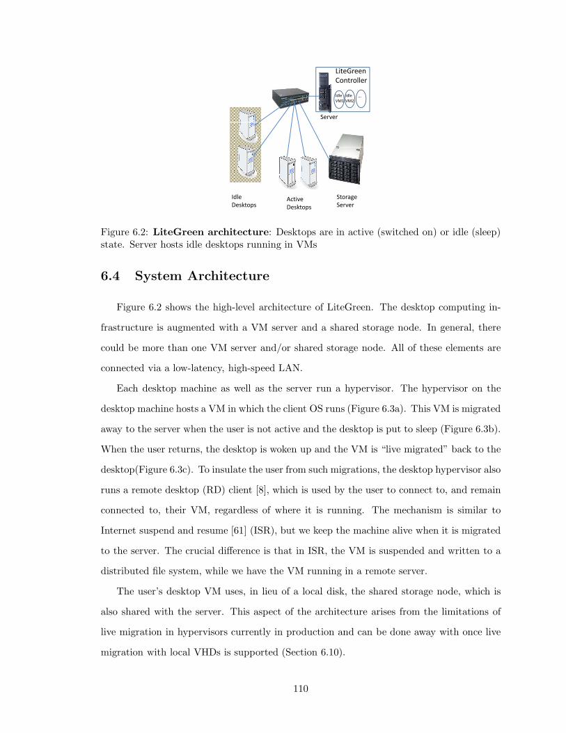
LiteGreen
CC
LiteGreen
Controller
Idle Idle … Idle
VM1
Idle
VM2
…
Server
Idle Active StorageIdle
DesktopsActive
Desktops
Storage
Server
Figure 6.2: LiteGreen architecture: Desktops are in active (switched on) or idle (sleep)state. Server hosts idle desktops running in VMs
6.4 System Architecture
Figure 6.2 shows the high-level architecture of LiteGreen. The desktop computing in-
frastructure is augmented with a VM server and a shared storage node. In general, there
could be more than one VM server and/or shared storage node. All of these elements are
connected via a low-latency, high-speed LAN.
Each desktop machine as well as the server run a hypervisor. The hypervisor on the
desktop machine hosts a VM in which the client OS runs (Figure 6.3a). This VM is migrated
away to the server when the user is not active and the desktop is put to sleep (Figure 6.3b).
When the user returns, the desktop is woken up and the VM is “live migrated” back to the
desktop(Figure 6.3c). To insulate the user from such migrations, the desktop hypervisor also
runs a remote desktop (RD) client [8], which is used by the user to connect to, and remain
connected to, their VM, regardless of where it is running. The mechanism is similar to
Internet suspend and resume [61] (ISR), but we keep the machine alive when it is migrated
to the server. The crucial difference is that in ISR, the VM is suspended and written to a
distributed file system, while we have the VM running in a remote server.
The user’s desktop VM uses, in lieu of a local disk, the shared storage node, which is
also shared with the server. This aspect of the architecture arises from the limitations of
live migration in hypervisors currently in production and can be done away with once live
migration with local VHDs is supported (Section 6.10).
110

(a) Virtualized
desktop: OS incurrent desktops isrun in a VM
(b) Idle VM on the server: Afterthe VM is migrated, desktop is put tosleep
(c) Migrating VM: While the VM isbeing migrated, RD client allows ac-cess to graphical desktop
Figure 6.3: Desktop states
The hypervisor on the server hosts the guest VMs that have been migrated to it from
(idle) desktop machines. The server also includes a controller, which is the brain of Lite-
Green. The controller receives periodic updates from stubs on the desktop hypervisors on
the level of user and computing activity on the desktops. The controller also tracks resource
usage on the server. Using all of this information, the controller orchestrates the migration
of VMs to the server and back to the desktop machines, and manages the allocation of
resources on the server.
6.5 Design
Having provided an overview of the architecture, we now detail the design of LiteGreen.
The design of LiteGreen has to deal with two somewhat conflicting goals: maximizing energy
savings from putting machines to sleep while minimizing disruption to users. When faced
with a choice, LiteGreen errs on the side of being conservative, i.e., avoiding user disruption
even if it means reduced energy savings.
The operation of LiteGreen can be described in terms of a control loop effected by the
controller based on local information at the server as well as information reported by the
desktop stubs. We discuss the individual elements before putting together the whole control
loop.
111
6.5.1 Which VMs to Migrate?
The controller maintains two lists of VMs:
• Eligible for Pull: list of (idle) VMs that currently reside on the desktop machines but
could be migrated (i.e., “pulled”) to the server, thereby saving energy without user
disruption.
• Mandatory to Push: list of (now active) VMs that had previously been migrated to
the server but must now be migrated (i.e., “pushed”) back to the desktop machines
at the earliest to minimize user disruption.
In general, the determination of whether a VM is active or idle is made based on both
UI activity initiated by the user and computing activity, as discussed next.
6.5.2 Determining If Idle or Active
The presence of any UI activity initiated by the user, through the mouse or the keyboard
(e.g., mouse movement, mouse clicks, key presses), in the recent past (actvityWindow, set to
10 minutes by default) is interpreted as an indicator that the machine is active. Even though
the load imposed on the machine might be rather minimal, we make this conservative choice
to reflect our emphasis on minimizing the impact on the interactive performance perceived
by the user.
In the default policy, the presence of UI activity is taken as the only indicator of whether
the machine is active. So, the absence of recent UI activity is taken as the machine is idle.
A more conservative policy, however, also considers the actual computational load on
the machine. Specifically, if the CPU usage is above a threshold, the machine is deemed to
be active. So, for the machine to be deemed idle, both the absence of recent UI activity and
CPU usage being below the threshold are necessary conditions. To avoid too much bouncing
between the active and idle states, we introduce hysteresis in the process by (a) measuring
the CPU usage as the average over an interval (e.g., 1 minute) rather than instantaneously,
and (b) having a higher threshold, cpush, for the push list (i.e., idle→active transition of
a VM currently on the server) than the threshold, cpull, for the pull list (i.e., for a VM
112
currently on a desktop machine).
6.5.3 Server Capacity Constraint
A second factor that the controller considers while making migration decisions is the
availability of resources on the server. If the server’s resources are saturated or close to
it, the controller migrates some VMs back to the desktop machines to relieve the pressure.
Thus, an idle VM is merely eligible for being consolidated on the server and, in fact, might
not be if the server does not have the capacity. On the other hand, an active VM must
be migrated back to the desktop machine even if the server has the capacity. This design
reflects the choice to err on the side of being conservative, as noted above.
There are two server resource constraints that we focus on. The first is memory avail-
ability. Given a total server memory, M , and the allocation, m, made to each VM, the
number of VMs that can be hosted on the server is bounded by nRAM = Mm
. Note that
m is the memory allocated to a VM after ballooning and would typically be some minimal
value such as 384 MB that allows an idle VM to still function (Section 6.8.4).
The second resource constraint arises from CPU usage. Basically, the aggregate CPU
usage of all the VMs on the server should be below a threshold. As with the conservative
client-side policy discussed in Section 6.5.2, we introduce hysteresis by (a) measuring the
CPU usage as the average over a time interval (e.g., 1 minute), and (b) having a higher
threshold, spush, for pushing out VMs, than the threshold, spull, for pulling in VMs. The
server tries to pull in VMs (assuming the pull list is non-empty) so long as the aggregate
CPU usage is under spull. Then, if the CPU usage rises above spush, the server pushes back
VMs. Thus, there is a bound, nCPU , on the number of VMs that can be accommodated
such that∑i=nCPU
i=1 xi ≤ spush, where xi is the CPU usage of the ith VM. Adding system
overhead to get a more accurate assessment of amount of CPU and memory required is left
as future work.
The total number of VMs that can be consolidated on the server is bounded by min(nRAM , nCPU).
While one could extend this mechanism to other resources such as network and disk, our
evaluation in Section 6.9 indicates that enforcing CPU constraints also ends up limiting the
usage of other resources.
113
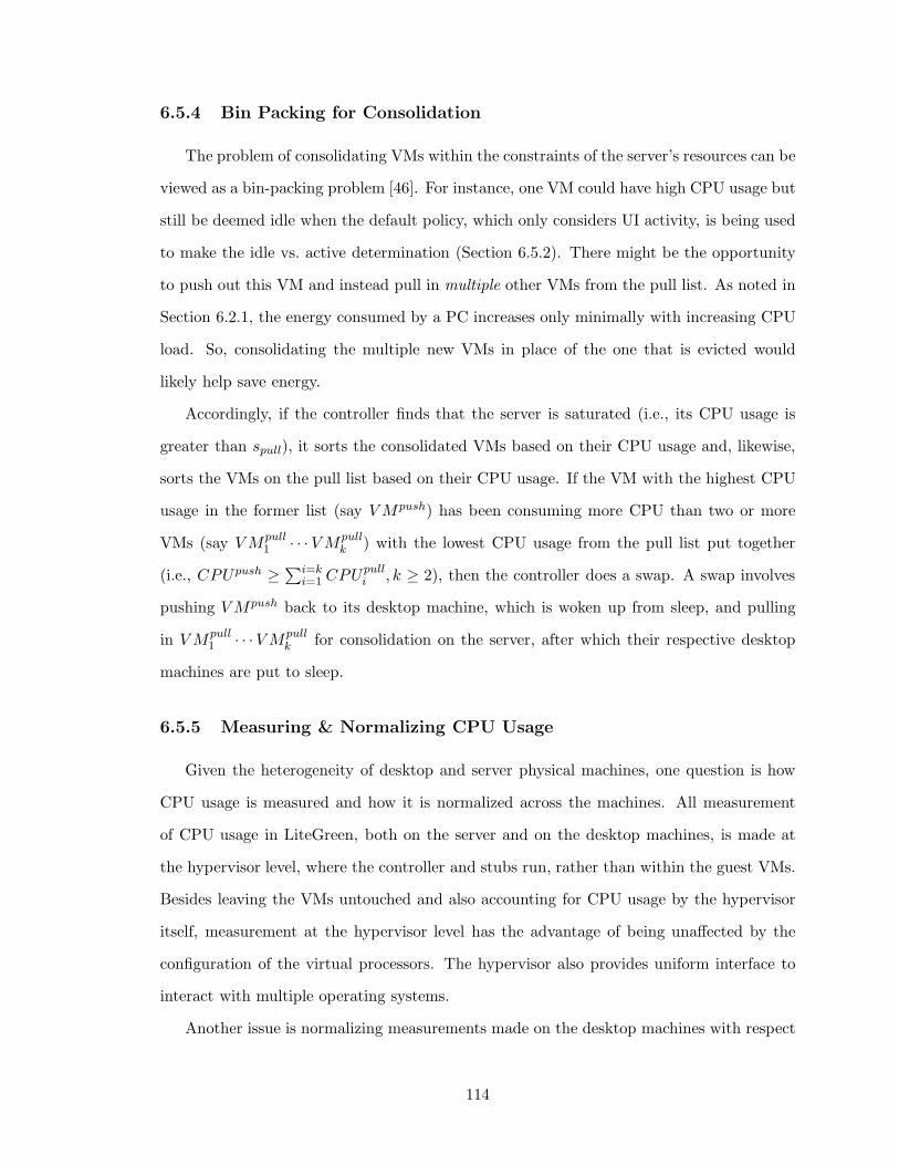
6.5.4 Bin Packing for Consolidation
The problem of consolidating VMs within the constraints of the server’s resources can be
viewed as a bin-packing problem [46]. For instance, one VM could have high CPU usage but
still be deemed idle when the default policy, which only considers UI activity, is being used
to make the idle vs. active determination (Section 6.5.2). There might be the opportunity
to push out this VM and instead pull in multiple other VMs from the pull list. As noted in
Section 6.2.1, the energy consumed by a PC increases only minimally with increasing CPU
load. So, consolidating the multiple new VMs in place of the one that is evicted would
likely help save energy.
Accordingly, if the controller finds that the server is saturated (i.e., its CPU usage is
greater than spull), it sorts the consolidated VMs based on their CPU usage and, likewise,
sorts the VMs on the pull list based on their CPU usage. If the VM with the highest CPU
usage in the former list (say V Mpush) has been consuming more CPU than two or more
VMs (say V Mpull1 · · · V Mpull
k ) with the lowest CPU usage from the pull list put together
(i.e., CPUpush ≥∑i=k
i=1 CPUpulli , k ≥ 2), then the controller does a swap. A swap involves
pushing V Mpush back to its desktop machine, which is woken up from sleep, and pulling
in V Mpull1 · · ·V Mpull
k for consolidation on the server, after which their respective desktop
machines are put to sleep.
6.5.5 Measuring & Normalizing CPU Usage
Given the heterogeneity of desktop and server physical machines, one question is how
CPU usage is measured and how it is normalized across the machines. All measurement
of CPU usage in LiteGreen, both on the server and on the desktop machines, is made at
the hypervisor level, where the controller and stubs run, rather than within the guest VMs.
Besides leaving the VMs untouched and also accounting for CPU usage by the hypervisor
itself, measurement at the hypervisor level has the advantage of being unaffected by the
configuration of the virtual processors. The hypervisor also provides uniform interface to
interact with multiple operating systems.
Another issue is normalizing measurements made on the desktop machines with respect
114
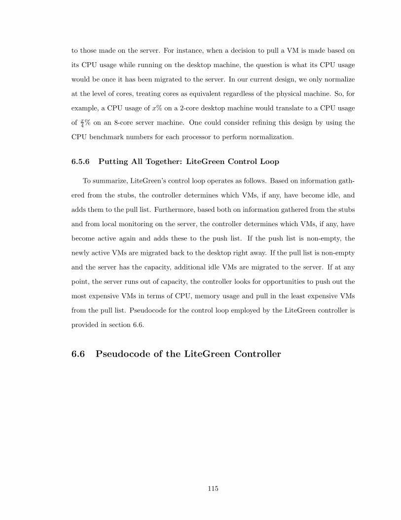
to those made on the server. For instance, when a decision to pull a VM is made based on
its CPU usage while running on the desktop machine, the question is what its CPU usage
would be once it has been migrated to the server. In our current design, we only normalize
at the level of cores, treating cores as equivalent regardless of the physical machine. So, for
example, a CPU usage of x% on a 2-core desktop machine would translate to a CPU usage
of x4% on an 8-core server machine. One could consider refining this design by using the
CPU benchmark numbers for each processor to perform normalization.
6.5.6 Putting All Together: LiteGreen Control Loop
To summarize, LiteGreen’s control loop operates as follows. Based on information gath-
ered from the stubs, the controller determines which VMs, if any, have become idle, and
adds them to the pull list. Furthermore, based both on information gathered from the stubs
and from local monitoring on the server, the controller determines which VMs, if any, have
become active again and adds these to the push list. If the push list is non-empty, the
newly active VMs are migrated back to the desktop right away. If the pull list is non-empty
and the server has the capacity, additional idle VMs are migrated to the server. If at any
point, the server runs out of capacity, the controller looks for opportunities to push out the
most expensive VMs in terms of CPU, memory usage and pull in the least expensive VMs
from the pull list. Pseudocode for the control loop employed by the LiteGreen controller is
provided in section 6.6.
6.6 Pseudocode of the LiteGreen Controller
115
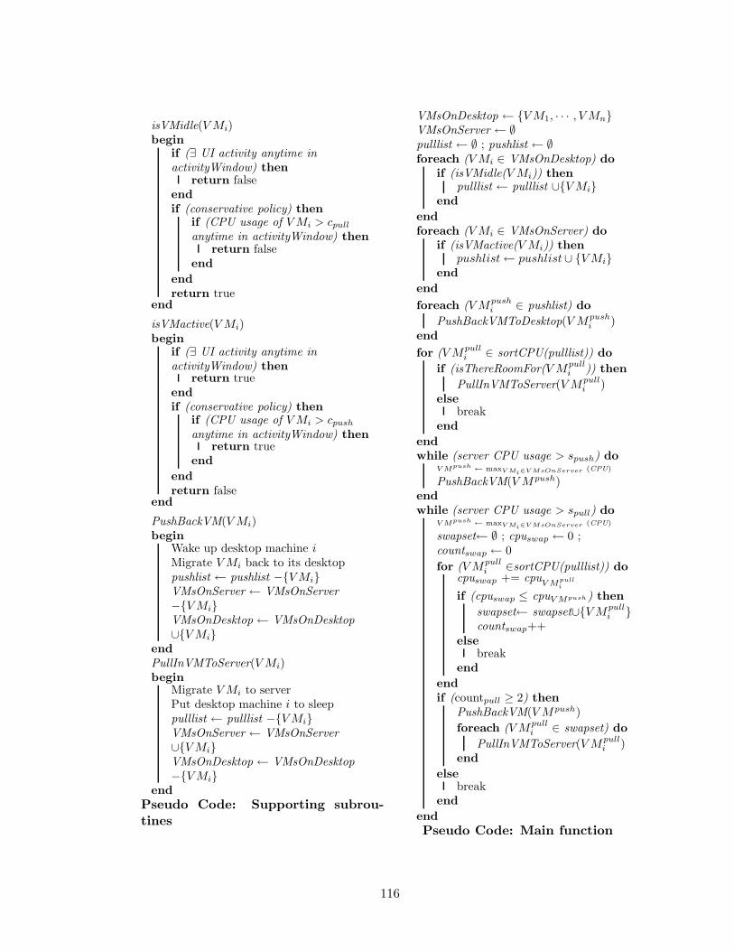
isVMidle(V Mi)begin
if (∃ UI activity anytime inactivityWindow) then
return falseendif (conservative policy) then
if (CPU usage of V Mi > cpull
anytime in activityWindow) thenreturn false
end
endreturn true
end
isVMactive(V Mi)begin
if (∃ UI activity anytime inactivityWindow) then
return trueendif (conservative policy) then
if (CPU usage of V Mi > cpush
anytime in activityWindow) thenreturn true
end
endreturn false
end
PushBackVM(V Mi)begin
Wake up desktop machine iMigrate V Mi back to its desktoppushlist ← pushlist −{V Mi}VMsOnServer ← VMsOnServer−{V Mi}VMsOnDesktop ← VMsOnDesktop∪{V Mi}
endPullInVMToServer(V Mi)begin
Migrate V Mi to serverPut desktop machine i to sleeppulllist ← pulllist −{V Mi}VMsOnServer ← VMsOnServer∪{V Mi}VMsOnDesktop ← VMsOnDesktop−{V Mi}
endPseudo Code: Supporting subrou-tines
VMsOnDesktop ← {V M1, · · · , V Mn}VMsOnServer ← ∅pulllist ← ∅ ; pushlist ← ∅foreach (V Mi ∈ VMsOnDesktop) do
if (isVMidle(V Mi)) thenpulllist ← pulllist ∪{V Mi}
end
endforeach (V Mi ∈ VMsOnServer) do
if (isVMactive(V Mi)) thenpushlist← pushlist∪ {V Mi}
end
end
foreach (V Mpushi ∈ pushlist) do
PushBackVMToDesktop(V Mpushi )
end
for (V Mpulli ∈ sortCPU(pulllist)) do
if (isThereRoomFor(V Mpulli )) then
PullInVMToServer(V Mpulli )
elsebreak
end
endwhile (server CPU usage > spush) do
V Mpush← maxV Mi∈V MsOnServer (CPU)
PushBackVM(V Mpush)endwhile (server CPU usage > spull) do
V Mpush← maxV Mi∈V MsOnServer (CPU)
swapset← ∅ ; cpuswap ← 0 ;countswap ← 0
for (V Mpulli ∈sortCPU(pulllist)) do
cpuswap += cpuV M
pull
i
if (cpuswap ≤ cpuV Mpush) then
swapset← swapset∪{V Mpulli }
countswap++else
breakend
endif (countpull ≥ 2) then
PushBackVM(V Mpush)
foreach (V Mpulli ∈ swapset) do
PullInVMToServer(V Mpulli )
end
elsebreak
end
endPseudo Code: Main function
116

6.7 Implementation and Deployment
We have built a prototype of LiteGreen based on the Hyper-V hypervisor, which is
available as part of the Microsoft Hyper-V Server 2008 R2 [4]. The Hyper-V server can
host Windows, Linux, and other guest OSes and also supports live migration.
Our implementation comprises the controller, which runs on the server, and the stubs,
which run on the individual desktop machines. The controller and stubs are written in
C# and add up to 1600 and 600 lines of code, respectively. The stubs use WMI (Windows
Management Instrumentation)[13] and Powershell to perform the monitoring and migration.
The controller also includes a GUI, which shows the state of all of the VMs in the system.
In our implementation, we ran into issues arising from the limitations of Hyper-V and
had to work around them. Here we discuss a couple of these.
Lack of support for sleep: Since Hyper-V is intended for use on servers, it does not
support sleep once the hypervisor service has been started. Also, once started, the hypervi-
sor service cannot be turned off without a reboot. We worked around this as follows: when
the desktop VM has been migrated away to the server and the desktop machine is to be
put to sleep, we set a registry key to disable the hypervisor and then reboot the machine.
When the machine boots up again, the hypervisor is no longer running, so the desktop
machine can be put to sleep. Later, when the user returns and the machine is woken up,
the hypervisor service is restarted, without requiring a reboot. Note that since a reboot is
needed only when the machine is put to sleep but not when it is woken up, the user does
not perceive any delay or disruption due to the reboot.
Surge in CPU usage right after live migration: We have found that for a period
of 2-3 minutes after the completion of live migration, there is a surge in the CPU usage
of the VM, with the VM saturating its virtual processor. This surge might be due to the
final copying phase of live migration, though no official documentation is available in this
regard. Nevertheless, the surge could potentially confuse the controller. In particular, if the
conservative policy is being used to determine whether a VM is active or idle (Section 6.5.2)
and if the VM has just been pulled into the server, the surge in CPU usage could trigger the
117

controller to incorrectly conclude that the VM is active again and push it back immediately.
We work around this in our implementation by adding a few minutes’ of hysteresis in the
controller’s control loop, thereby allowing time for the surge to subside.
6.7.1 Deployment
We have deployed LiteGreen to 5 users at MSR India. Each user has LiteGreen installed
on a second desktop machine, which is in addition to their existing desktop machine that
is left untouched.
Different users use their LiteGreen desktop machine in different ways. Some use it only
for specific tasks, such as browsing or checking email, so that the LiteGreen desktop only
sees a subset of their activity. Others use it for all of their computing activity, including
connecting to their existing desktop machine through their LiteGreen desktop. Our findings
are reported in Section 6.8.3. While our deployment is very small in size and moreover, has
not entirely replaced the users’ existing desktop machines, we believe it is a valuable first
step that we plan to build on in future.
6.8 Evaluation Results
We begin by presenting experimental results based on our prototype. These results are
drawn both from controlled experiments in the lab and from our deployment. The results
are, however, limited by the small scale of our testbed and deployment, so in Section 6.9
we present a larger scale trace-driven evaluation using the traces gathered from the 120
machines at our lab.
6.8.1 Testbed
Our testbed mirrors the architecture depicted in Figure 6.2. It comprises 5 desktop
machines, a server, and a storage node, all connected to a GigE switch. The hardware and
software details are listed in Table 6.2.
We first used the testbed for controlled experiments in the lab (Section 6.8.2). We
then used the same setup but with the desktop machines installed in the offices of the
118
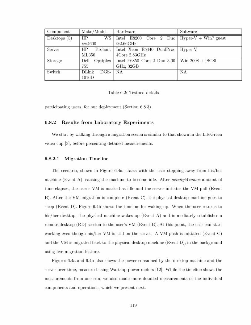
Component Make/Model Hardware Software
Desktops (5) HP WSxw4600
Intel E8200 Core 2 [email protected]
Hyper-V + Win7 guest
Server HP ProliantML350
Intel Xeon E5440 DualProc4Core 2.83GHz
Hyper-V
Storage Dell Optiplex755
Intel E6850 Core 2 Duo 3.00GHz, 32GB
Win 2008 + iSCSI
Switch DLink DGS-1016D
NA NA
Table 6.2: Testbed details
participating users, for our deployment (Section 6.8.3).
6.8.2 Results from Laboratory Experiments
We start by walking through a migration scenario similar to that shown in the LiteGreen
video clip [3], before presenting detailed measurements.
6.8.2.1 Migration Timeline
The scenario, shown in Figure 6.4a, starts with the user stepping away from his/her
machine (Event A), causing the machine to become idle. After actvityWindow amount of
time elapses, the user’s VM is marked as idle and the server initiates the VM pull (Event
B). After the VM migration is complete (Event C), the physical desktop machine goes to
sleep (Event D). Figure 6.4b shows the timeline for waking up. When the user returns to
his/her desktop, the physical machine wakes up (Event A) and immediately establishes a
remote desktop (RD) session to the user’s VM (Event B). At this point, the user can start
working even though his/her VM is still on the server. A VM push is initiated (Event C)
and the VM is migrated back to the physical desktop machine (Event D), in the background
using live migration feature.
Figures 6.4a and 6.4b also shows the power consumed by the desktop machine and the
server over time, measured using Wattsup power meters [12]. While the timeline shows the
measurements from one run, we also made more detailed measurements of the individual
components and operations, which we present next.
119
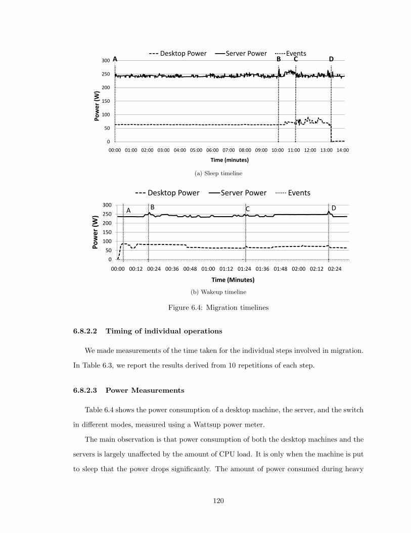
A B C D
250
300
Desktop Power Server Power EventsA B C D
50
100
150
200
250
300
Po
we
r (W
)
Desktop Power Server Power EventsA B C D
0
50
100
150
200
250
300
00:00 01:00 02:00 03:00 04:00 05:00 06:00 07:00 08:00 09:00 10:00 11:00 12:00 13:00 14:00
Po
we
r (W
)
Time (minutes)
Desktop Power Server Power EventsA B C D
0
50
100
150
200
250
300
00:00 01:00 02:00 03:00 04:00 05:00 06:00 07:00 08:00 09:00 10:00 11:00 12:00 13:00 14:00
Po
we
r (W
)
Time (minutes)
Desktop Power Server Power EventsA B C D
0
50
100
150
200
250
300
00:00 01:00 02:00 03:00 04:00 05:00 06:00 07:00 08:00 09:00 10:00 11:00 12:00 13:00 14:00
Po
we
r (W
)
Time (minutes)
Desktop Power Server Power EventsA B C D
0
50
100
150
200
250
300
00:00 01:00 02:00 03:00 04:00 05:00 06:00 07:00 08:00 09:00 10:00 11:00 12:00 13:00 14:00
Po
we
r (W
)
Time (minutes)
Desktop Power Server Power Events
(a) Sleep timeline
300
Desktop Power Server Power Events
AB C D
50
100
150
200
250
300
Po
we
r (W
)
Desktop Power Server Power Events
AB C D
0
50
100
150
200
250
300
00:00 00:12 00:24 00:36 00:48 01:00 01:12 01:24 01:36 01:48 02:00 02:12 02:24
Po
we
r (W
)
Time (Minutes)
Desktop Power Server Power Events
AB C D
0
50
100
150
200
250
300
00:00 00:12 00:24 00:36 00:48 01:00 01:12 01:24 01:36 01:48 02:00 02:12 02:24
Po
we
r (W
)
Time (Minutes)
Desktop Power Server Power Events
AB C D
0
50
100
150
200
250
300
00:00 00:12 00:24 00:36 00:48 01:00 01:12 01:24 01:36 01:48 02:00 02:12 02:24
Po
we
r (W
)
Time (Minutes)
Desktop Power Server Power Events
AB C D
0
50
100
150
200
250
300
00:00 00:12 00:24 00:36 00:48 01:00 01:12 01:24 01:36 01:48 02:00 02:12 02:24
Po
we
r (W
)
Time (Minutes)
Desktop Power Server Power Events
AB C D
(b) Wakeup timeline
Figure 6.4: Migration timelines
6.8.2.2 Timing of individual operations
We made measurements of the time taken for the individual steps involved in migration.
In Table 6.3, we report the results derived from 10 repetitions of each step.
6.8.2.3 Power Measurements
Table 6.4 shows the power consumption of a desktop machine, the server, and the switch
in different modes, measured using a Wattsup power meter.
The main observation is that power consumption of both the desktop machines and the
servers is largely unaffected by the amount of CPU load. It is only when the machine is put
to sleep that the power drops significantly. The amount of power consumed during heavy
120
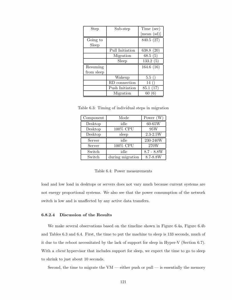
Step Sub-step Time (sec)[mean (sd)]
Going to 840.5 (27)Sleep
Pull Initiation 638.8 (20)
Migration 68.5 (5)
Sleep 133.2 (5)
Resuming 164.6 (16)from sleep
Wakeup 5.5 ()
RD connection 14 ()
Push Initiation 85.1 (17)
Migration 60 (6)
Table 6.3: Timing of individual steps in migration
Component Mode Power (W)
Desktop idle 60-65W
Desktop 100% CPU 95W
Desktop sleep 2.3-2.5W
Server idle 230-240W
Server 100% CPU 270W
Switch idle 8.7 - 8.8W
Switch during migration 8.7-8.8W
Table 6.4: Power measurements
load and low load in desktops or servers does not vary much because current systems are
not energy proportional systems. We also see that the power consumption of the network
switch is low and is unaffected by any active data transfers.
6.8.2.4 Discussion of the Results
We make several observations based on the timeline shown in Figure 6.4a, Figure 6.4b
and Tables 6.3 and 6.4. First, the time to put the machine to sleep is 133 seconds, much of
it due to the reboot necessitated by the lack of support for sleep in Hyper-V (Section 6.7).
With a client hypervisor that includes support for sleep, we expect the time to go to sleep
to shrink to just about 10 seconds.
Second, the time to migrate the VM — either push or pull — is essentially the memory
121
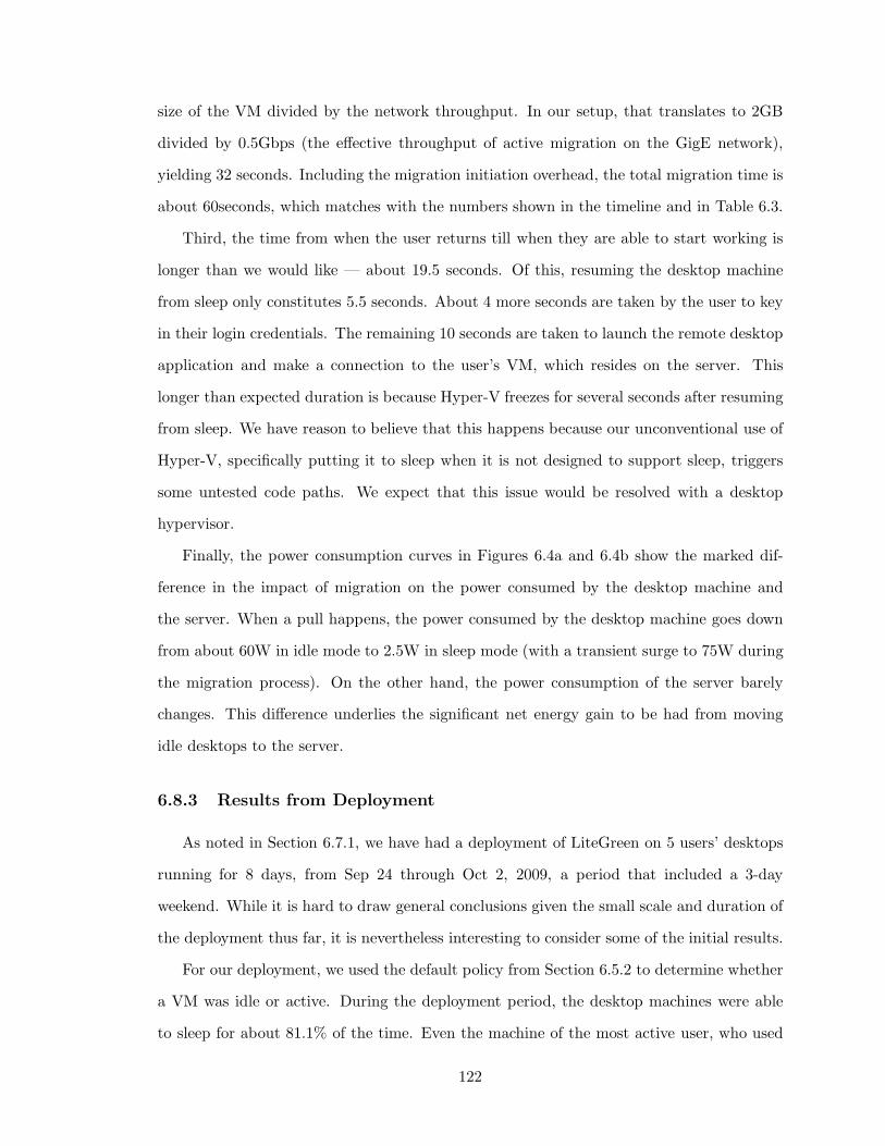
size of the VM divided by the network throughput. In our setup, that translates to 2GB
divided by 0.5Gbps (the effective throughput of active migration on the GigE network),
yielding 32 seconds. Including the migration initiation overhead, the total migration time is
about 60seconds, which matches with the numbers shown in the timeline and in Table 6.3.
Third, the time from when the user returns till when they are able to start working is
longer than we would like — about 19.5 seconds. Of this, resuming the desktop machine
from sleep only constitutes 5.5 seconds. About 4 more seconds are taken by the user to key
in their login credentials. The remaining 10 seconds are taken to launch the remote desktop
application and make a connection to the user’s VM, which resides on the server. This
longer than expected duration is because Hyper-V freezes for several seconds after resuming
from sleep. We have reason to believe that this happens because our unconventional use of
Hyper-V, specifically putting it to sleep when it is not designed to support sleep, triggers
some untested code paths. We expect that this issue would be resolved with a desktop
hypervisor.
Finally, the power consumption curves in Figures 6.4a and 6.4b show the marked dif-
ference in the impact of migration on the power consumed by the desktop machine and
the server. When a pull happens, the power consumed by the desktop machine goes down
from about 60W in idle mode to 2.5W in sleep mode (with a transient surge to 75W during
the migration process). On the other hand, the power consumption of the server barely
changes. This difference underlies the significant net energy gain to be had from moving
idle desktops to the server.
6.8.3 Results from Deployment
As noted in Section 6.7.1, we have had a deployment of LiteGreen on 5 users’ desktops
running for 8 days, from Sep 24 through Oct 2, 2009, a period that included a 3-day
weekend. While it is hard to draw general conclusions given the small scale and duration of
the deployment thus far, it is nevertheless interesting to consider some of the initial results.
For our deployment, we used the default policy from Section 6.5.2 to determine whether
a VM was idle or active. During the deployment period, the desktop machines were able
to sleep for about 81.1% of the time. Even the machine of the most active user, who used
122
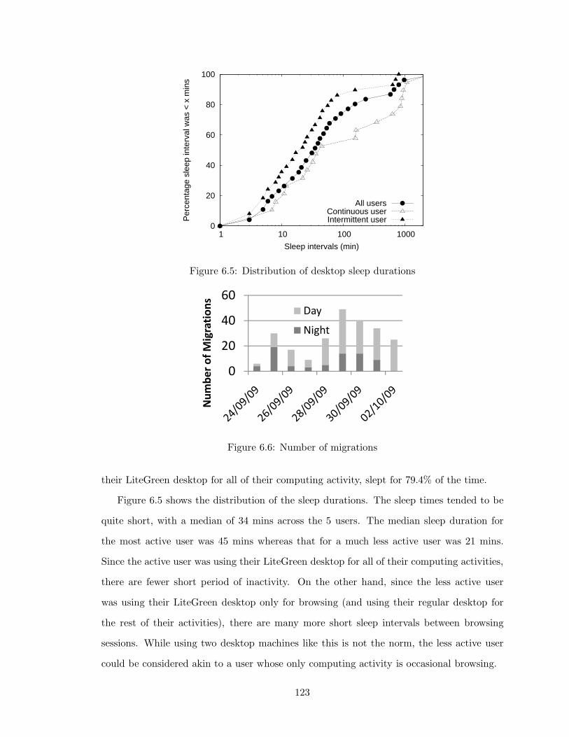
0
20
40
60
80
100
1 10 100 1000
Per
cent
age
slee
p in
terv
al w
as <
x m
ins
Sleep intervals (min)
All usersContinuous userIntermittent user
Figure 6.5: Distribution of desktop sleep durations
40
60
Nu
mb
er
of
Mig
rati
on
s
Day
Night
0
20
40
60
Nu
mb
er
of
Mig
rati
on
s
Day
Night
0
20
40
60
Nu
mb
er
of
Mig
rati
on
s
Day
Night
0
20
40
60
Nu
mb
er
of
Mig
rati
on
s
Day
Night
0
20
40
60
Nu
mb
er
of
Mig
rati
on
s
Day
Night
0
20
40
60
Nu
mb
er
of
Mig
rati
on
s
Day
Night
Figure 6.6: Number of migrations
their LiteGreen desktop for all of their computing activity, slept for 79.4% of the time.
Figure 6.5 shows the distribution of the sleep durations. The sleep times tended to be
quite short, with a median of 34 mins across the 5 users. The median sleep duration for
the most active user was 45 mins whereas that for a much less active user was 21 mins.
Since the active user was using their LiteGreen desktop for all of their computing activities,
there are fewer short period of inactivity. On the other hand, since the less active user
was using their LiteGreen desktop only for browsing (and using their regular desktop for
the rest of their activities), there are many more short sleep intervals between browsing
sessions. While using two desktop machines like this is not the norm, the less active user
could be considered akin to a user whose only computing activity is occasional browsing.
123
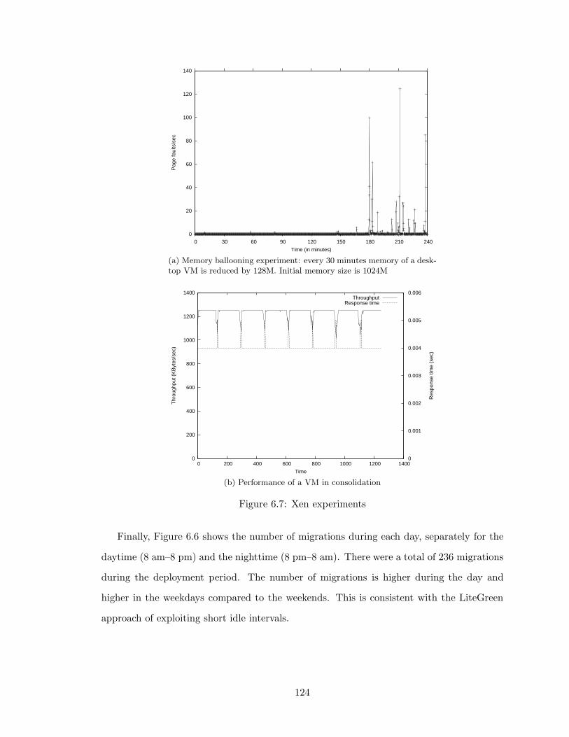
0
20
40
60
80
100
120
140
0 30 60 90 120 150 180 210 240
Pag
e fa
ults
/sec
Time (in minutes)
(a) Memory ballooning experiment: every 30 minutes memory of a desk-top VM is reduced by 128M. Initial memory size is 1024M
0
200
400
600
800
1000
1200
1400
0 200 400 600 800 1000 1200 1400 0
0.001
0.002
0.003
0.004
0.005
0.006
Thr
ough
put (
KB
ytes
/sec
)
Res
pons
e tim
e (s
ec)
Time
ThroughputResponse time
(b) Performance of a VM in consolidation
Figure 6.7: Xen experiments
Finally, Figure 6.6 shows the number of migrations during each day, separately for the
daytime (8 am–8 pm) and the nighttime (8 pm–8 am). There were a total of 236 migrations
during the deployment period. The number of migrations is higher during the day and
higher in the weekdays compared to the weekends. This is consistent with the LiteGreen
approach of exploiting short idle intervals.
124
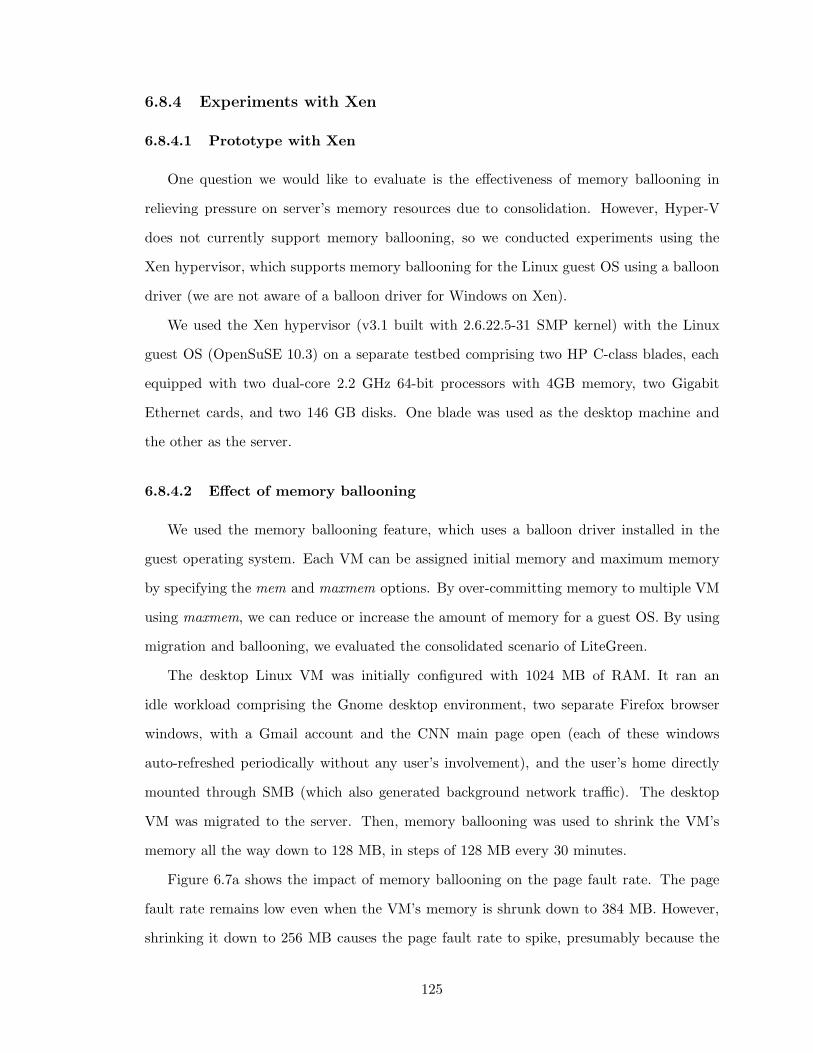
6.8.4 Experiments with Xen
6.8.4.1 Prototype with Xen
One question we would like to evaluate is the effectiveness of memory ballooning in
relieving pressure on server’s memory resources due to consolidation. However, Hyper-V
does not currently support memory ballooning, so we conducted experiments using the
Xen hypervisor, which supports memory ballooning for the Linux guest OS using a balloon
driver (we are not aware of a balloon driver for Windows on Xen).
We used the Xen hypervisor (v3.1 built with 2.6.22.5-31 SMP kernel) with the Linux
guest OS (OpenSuSE 10.3) on a separate testbed comprising two HP C-class blades, each
equipped with two dual-core 2.2 GHz 64-bit processors with 4GB memory, two Gigabit
Ethernet cards, and two 146 GB disks. One blade was used as the desktop machine and
the other as the server.
6.8.4.2 Effect of memory ballooning
We used the memory ballooning feature, which uses a balloon driver installed in the
guest operating system. Each VM can be assigned initial memory and maximum memory
by specifying the mem and maxmem options. By over-committing memory to multiple VM
using maxmem, we can reduce or increase the amount of memory for a guest OS. By using
migration and ballooning, we evaluated the consolidated scenario of LiteGreen.
The desktop Linux VM was initially configured with 1024 MB of RAM. It ran an
idle workload comprising the Gnome desktop environment, two separate Firefox browser
windows, with a Gmail account and the CNN main page open (each of these windows
auto-refreshed periodically without any user’s involvement), and the user’s home directly
mounted through SMB (which also generated background network traffic). The desktop
VM was migrated to the server. Then, memory ballooning was used to shrink the VM’s
memory all the way down to 128 MB, in steps of 128 MB every 30 minutes.
Figure 6.7a shows the impact of memory ballooning on the page fault rate. The page
fault rate remains low even when the VM’s memory is shrunk down to 384 MB. However,
shrinking it down to 256 MB causes the page fault rate to spike, presumably because the
125

working set no longer fits within memory.
It is interesting, though, that beyond the initial spike, the page fault rate remains low
during the rest of the 30-minute period even with the memory set to 256 MB.
We conclude that in our setup with the idle workload that we used, memory ballooning
could be used to shrink the memory of an idle VM by almost a factor of 3 (1024 MB
down to 384 MB), without causing thrashing. Further savings in memory could be achieved
through memory sharing. While we were not able to evaluate this in our testbed since
neither Hyper-V nor Xen supports it, the findings from prior work [51] are encouraging, as
discussed in Section 6.10.
6.8.4.3 Consolidation of multiple VMs
To evaluate the consolidation of VMs, we again used two blades. A desktop Linux
VM is started on one of the blades, migrated and ballooned. A workload representing idle
desktop workload is run in the VM. This workload is generated using a micro benchmark
that follows an idle desktop trace from our data collection. The micro benchmark runs a
set of operations based on amount of resource to be consumed. For example, to consume
50% CPU, it would run 5000 operations and so on.
After 200 seconds, a second desktop running another idle workload is migrated and
ballooned into the server. We continue to migrate the idle desktops until no memory is left.
Figure 6.7b shows the performance of the first desktop VM. You can see that there are
a few blips in performance whenever a new desktop is migrated.
6.9 Simulation
To evaluate our algorithms further, we have built a discrete event simulator written
in Python using the SimPy package. The simulator runs through the desktop traces, and
simulates the default and conservative policies based on various parameters including cpull,
cpush, spull, spush and ServerCapacity. In the rest of the section, we will report on energy
savings achieved by LiteGreen and utilization of various resources (CPU, network, disk) at
the server as a result of consolidation of the idle desktop VMs.
126

90
100
Weekend Night
21.374.48
5.72
5.32
6.79
60
70
80
90
100
Weekend Night
Weekend Day
WeekNight
WeekDay
11.9817.91
15.65
21.374.48
5.72
7.23
5.32
6.79
30
40
50
60
70
80
90
100
Savings
Weekend Night
Weekend Day
WeekNight
WeekDay
6.63
11.9817.91
17.38
15.65
21.37
4.66
4.48
5.72
7.23
5.32
6.79
10
20
30
40
50
60
70
80
90
100
Savings
Weekend Night
Weekend Day
WeekNight
WeekDay
6.63
11.9817.91
17.38
15.65
21.37
4.66
4.48
5.72
7.23
5.32
6.79
0
10
20
30
40
50
60
70
80
90
100
Existing LiteGreen
Conservative
LiteGreen
Default
Savings
Weekend Night
Weekend Day
WeekNight
WeekDay
6.63
11.9817.91
17.38
15.65
21.37
4.66
4.48
5.72
7.23
5.32
6.79
0
10
20
30
40
50
60
70
80
90
100
Existing LiteGreen
Conservative
LiteGreen
Default
Savings
Weekend Night
Weekend Day
WeekNight
WeekDay
6.63
11.9817.91
17.38
15.65
21.37
4.66
4.48
5.72
7.23
5.32
6.79
0
10
20
30
40
50
60
70
80
90
100
Existing LiteGreen
Conservative
LiteGreen
Default
Savings
Weekend Night
Weekend Day
WeekNight
WeekDay
(a) Energy savings
80
90
100
Weekend Night
Weekend Day
1.864.3
0.1
3.34
0
4.52
60
70
80
90
100
Weekend Night
Weekend Day
WeekNight
WeekDay2.05 4.731.86
4.3
5.12
0.1
3.34
7.23
0
4.52
30
40
50
60
70
80
90
100
Savings
Weekend Night
Weekend Day
WeekNight
WeekDay2.05 4.73
34.18
1.864.3
5.12
0.1
3.34
7.23
0
4.52
10
20
30
40
50
60
70
80
90
100
Savings
Weekend Night
Weekend Day
WeekNight
WeekDay
6.19
2.05 4.73
34.18
1.864.3
5.12
0.1
3.34
7.23
0
4.52
0
10
20
30
40
50
60
70
80
90
100
Existing LiteGreen
Conservative
LiteGreen
Default
Savings
Weekend Night
Weekend Day
WeekNight
WeekDay
6.19
2.05 4.73
34.18
1.864.3
5.12
0.1
3.34
7.23
0
4.52
0
10
20
30
40
50
60
70
80
90
100
Existing LiteGreen
Conservative
LiteGreen
Default
Savings
Weekend Night
Weekend Day
WeekNight
WeekDay
6.19
2.05 4.73
34.18
1.864.3
5.12
0.1
3.34
7.23
0
4.52
0
10
20
30
40
50
60
70
80
90
100
Existing LiteGreen
Conservative
LiteGreen
Default
Savings
Weekend Night
Weekend Day
WeekNight
WeekDay
(b) Energy savings for user1
100
Weekend Night
11.8112.48
60
70
80
90
100
Weekend Night
Weekend Day
WeekNight
29.81
9.3310.07
9.3310.07
11.8112.48
30
40
50
60
70
80
90
100
Savings
Weekend Night
Weekend Day
WeekNight
WeekDay
1.8
26.37 29.81
2.36
9.3310.07
2.36
9.3310.07
7.23
11.8112.48
0
10
20
30
40
50
60
70
80
90
100
Savings
Weekend Night
Weekend Day
WeekNight
WeekDay
1.8
26.37 29.81
2.36
9.3310.07
2.36
9.3310.07
7.23
11.8112.48
0
10
20
30
40
50
60
70
80
90
100
Existing LiteGreen Conservative LiteGreen Default
Savings
Weekend Night
Weekend Day
WeekNight
WeekDay
1.8
26.37 29.81
2.36
9.3310.07
2.36
9.3310.07
7.23
11.8112.48
0
10
20
30
40
50
60
70
80
90
100
Existing LiteGreen Conservative LiteGreen Default
Savings
Weekend Night
Weekend Day
WeekNight
WeekDay
1.8
26.37 29.81
2.36
9.3310.07
2.36
9.3310.07
7.23
11.8112.48
0
10
20
30
40
50
60
70
80
90
100
Existing LiteGreen Conservative LiteGreen Default
Savings
Weekend Night
Weekend Day
WeekNight
WeekDay
(c) Energy savings for user2
Figure 6.8: Energy savings from existing power management and LiteGreen’s default andconservative policies
127
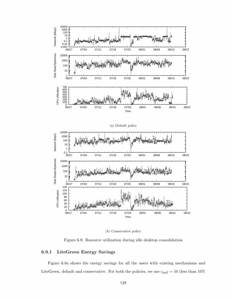
0 100 200 300 400 500 600 700
06/27 07/04 07/11 07/18 07/25 08/01 08/08 08/15 08/22
CP
U U
tiliz
atio
n
Time
1
10
100
1000
10000
06/27 07/04 07/11 07/18 07/25 08/01 08/08 08/15 08/22Dis
k R
ead
Byt
es/s
ec
0.001 0.01 0.1
1 10
100 1000
10000
06/27 07/04 07/11 07/18 07/25 08/01 08/08 08/15 08/22
Net
wor
k (M
bps)
(a) Default policy
0 20 40 60 80
100 120 140
06/27 07/04 07/11 07/18 07/25 08/01 08/08 08/15 08/22
CP
U U
tiliz
atio
n
Time
1
10
100
1000
10000
06/27 07/04 07/11 07/18 07/25 08/01 08/08 08/15 08/22Dis
k R
eads
Byt
es/s
ec
0.1
1
10
100
1000
10000
06/27 07/04 07/11 07/18 07/25 08/01 08/08 08/15 08/22
Net
wor
k (k
bps)
(b) Conservative policy
Figure 6.9: Resource utilization during idle desktop consolidation
6.9.1 LiteGreen Energy Savings
Figure 6.8a shows the energy savings for all the users with existing mechanisms and
LiteGreen, default and conservative. For both the policies, we use cpull = 10 (less than 10%
128
desktop usage classified as idle), cpush = 20, spull = 600, spush = 700 and ServerCapacity =
800 intended to represent a Server with 8 CPU cores.
As mentioned earlier, our desktop trace gathering tool records a number of parameters,
including CPU, memory, UI activity, disk, network, etc. every minute after its installation.
In order to estimate energy savings using existing mechanisms (either automatic windows
power management or manual desktop sleep by the user), we attribute any unrecorded
interval or “gaps” in our desktop trace to energy savings via existing mechanisms. Using
this technique, we estimate that existing mechanisms would have saved 35.2% of desktop
energy.
We then simulate the migrations of desktop VMs to/from the server depending on the
desktop trace events and the above mentioned thresholds for the conservative and default
policy. Using the conservative policy, we find that LiteGreen saves 37.3% of desktop energy.
This is in addition to the existing savings, for a total savings of 72%. If we use the more
aggressive default policy, where the desktop VM is migrated to the server unless there is
UI activity, we find that LiteGreen saves 51.3% on top of the existing 35.2% of savings
for a total savings of 86%. In the savings masurement, we assume that the desktop power
consumption is the same irrespective of the load on the machine. Power measurements done
by using tools like WattsUpMeter [12] can be used to more accurately measure the savings
for certain load.
The savings of the different approaches are also classified by day (8AM-8PM) and night
(8PM-8AM) and also whether it was a weekday or a weekend. We note that substantial
portion of LiteGreen savings comes from weekdays, thereby highlighting the importance of
exploiting short idle intervals in desktop energy savings.
6.9.2 Resource Utilization During Consolidation
While the default policy provides higher savings than the conservative policy, it is clear
that the default policy would stress the resources on the server more, due to hosting of a
higher number of desktop VMs, than the conservative policy. We examine this issue next.
Figures 6.9a and 6.9b show the resource utilization due to idle desktop consolidation at
the server for the default and conservative policies, respectively. The resources shown are
129

CPU usage, Bytes read/second from the disk, and network usage in Mbps.
First consider CPU. Notice that the CPU usage at the server in the default policy
spikes up to between spull = 600 an spush = 700 but, as intended, never goes above spush.
In contrast, since the conservative policy pushes the VM back to the desktop as soon as
cpush = 20 is exceeded, the CPU usage at the server hardly exceeds a utilization value of 100.
Next consider Disk Reads. It varies between 10B-10KB/s for the default policy (average
of 205 B/s ) while it varies between 10B-1KB/s for the conservative policy (average of 41
B/s). While these numbers can be quite easily managed by the server, note that these are
disk reads of idle, and not active, desktop VMs. Finally, let us consider network activity of
the consolidated idle desktop VMs. For the default policy, the network traffic mostly varies
between 0.01 to 10Mbps, but with occasional spikes all the way up to 10Gbps. In the case
of conservative policy, the network traffic does not exceed 10Mbps and rarely goes above
1Mbps. While these network traffic numbers are manageable by a server, scaling the server
for consolidation of active desktop VMs, as in the thin client model, will likely be expensive.
6.9.3 Energy Savings for Selected Users
Figure 6.10a and 6.10b depict the CPU utilization for two specific users. It appears
user1 has bursts of significant activity separated by periods of no activity, likely because
he/she manually switches off his/her machine when not in use as can be seen by the large
gaps in Figure 6.10a. For this particular case, LiteGreen is unable to significantly improve
the savings of existing mechanisms (including savings due to manual power management).
This is reflected in the energy savings for user1 in Figure 6.8b. In contrast, we see that
user2’s desktop has activity almost continuously, with only short gaps of inactivity. The
small CPU utilization spikes appears to have prevented Windows power management from
putting the desktop to sleep, thereby wasting a lot of energy. However, LiteGreen is able
to exploit this situation effectively, and saves a significant amount of energy as shown in
Figure 6.8c.
130
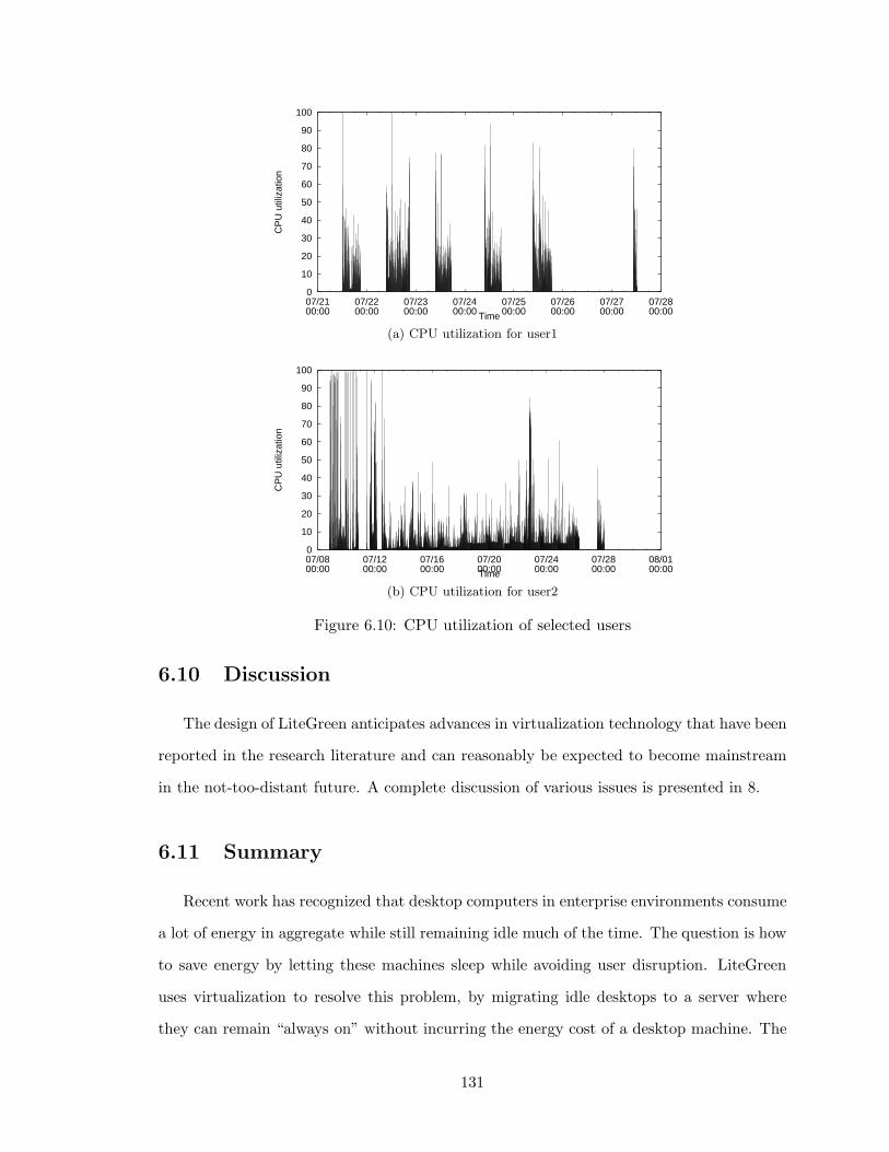
0
10
20
30
40
50
60
70
80
90
100
07/2100:00
07/2200:00
07/2300:00
07/2400:00
07/2500:00
07/2600:00
07/2700:00
07/2800:00
CP
U u
tiliz
atio
n
Time
(a) CPU utilization for user1
0
10
20
30
40
50
60
70
80
90
100
07/0800:00
07/1200:00
07/1600:00
07/2000:00
07/2400:00
07/2800:00
08/0100:00
CP
U u
tiliz
atio
n
Time
(b) CPU utilization for user2
Figure 6.10: CPU utilization of selected users
6.10 Discussion
The design of LiteGreen anticipates advances in virtualization technology that have been
reported in the research literature and can reasonably be expected to become mainstream
in the not-too-distant future. A complete discussion of various issues is presented in 8.
6.11 Summary
Recent work has recognized that desktop computers in enterprise environments consume
a lot of energy in aggregate while still remaining idle much of the time. The question is how
to save energy by letting these machines sleep while avoiding user disruption. LiteGreen
uses virtualization to resolve this problem, by migrating idle desktops to a server where
they can remain “always on” without incurring the energy cost of a desktop machine. The
131
seamlessness offered by LiteGreen allows us to aggressively exploit short idle periods as well
as long periods. Data-driven analysis of more than 65000 hours of desktop usage traces
from 120 users shows that LiteGreen can help desktops sleep for 72-86% of the time and
also scales well. The experience from our small-scale deployment of LiteGreen has also been
encouraging.
As the next step, we plan to expand our deployment. In future work, we plan to study
local disk migration, memory optimizations and extending it to multiple VM servers.
132
CHAPTER 7
Performance Evaluation of Server Consolidation in Xen and
OpenVZ
7.1 Introduction
There has been a rapid growth in servers within data centers driven by growth of enter-
prises since the late nineties. The servers are commonly used for running business-critical
applications such as enterprise resource planning, database, customer relationship manage-
ment, and e-commerce applications. Because these servers and applications involve high
labor cost in maintenance, upgrades, and operation, there is a significant interest in reduc-
ing the number of servers necessary for the applications. This strategy is supported by the
fact that many servers in enterprise data centers are under-utilized most of the time, with
a typical average utilization below 30%. On the other hand, some servers in a data center
may also become overloaded under peak demands, resulting in lower application throughput
and longer latency.
Server consolidation has become a common practice in enterprise data centers because
of the need to cut cost and increase return on IT investment. Many enterprise applications
that traditionally ran on dedicated servers are consolidated onto a smaller and shared pool of
servers. Although server consolidation offers great potential to increase resource utilization
and improve application performance, it may also introduce new complexity in managing the
consolidated servers. This has given rise to a re-surging interest in virtualization technology.
There are two main types of virtualization technologies today — hypervisor-based technology
133
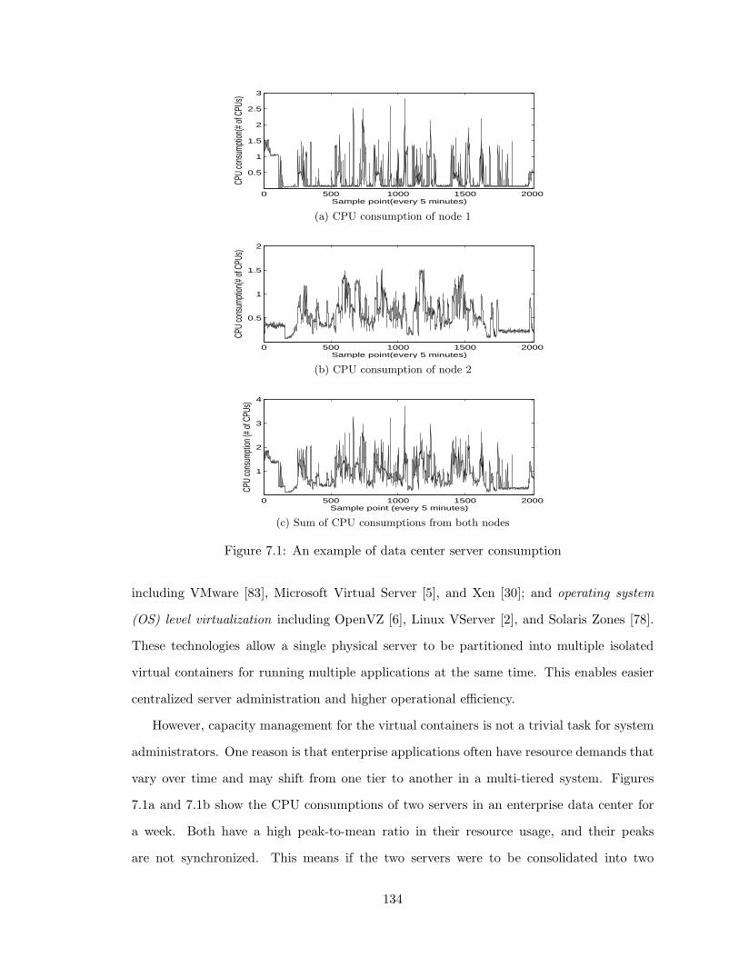
0 500 1000 1500 2000
0.5
1
1.5
2
2.5
3
Sample point(every 5 minutes)
CPU
cons
umpti
on(#
of C
PUs)
(a) CPU consumption of node 1
0 500 1000 1500 2000
0.5
1
1.5
2
Sample point(every 5 minutes)
CPU
cons
umpti
on(#
of C
PUs)
(b) CPU consumption of node 2
0 500 1000 1500 2000
1
2
3
4
Sample point (every 5 minutes)
CPU
cons
umpti
on (#
of C
PUs)
(c) Sum of CPU consumptions from both nodes
Figure 7.1: An example of data center server consumption
including VMware [83], Microsoft Virtual Server [5], and Xen [30]; and operating system
(OS) level virtualization including OpenVZ [6], Linux VServer [2], and Solaris Zones [78].
These technologies allow a single physical server to be partitioned into multiple isolated
virtual containers for running multiple applications at the same time. This enables easier
centralized server administration and higher operational efficiency.
However, capacity management for the virtual containers is not a trivial task for system
administrators. One reason is that enterprise applications often have resource demands that
vary over time and may shift from one tier to another in a multi-tiered system. Figures
7.1a and 7.1b show the CPU consumptions of two servers in an enterprise data center for
a week. Both have a high peak-to-mean ratio in their resource usage, and their peaks
are not synchronized. This means if the two servers were to be consolidated into two
134
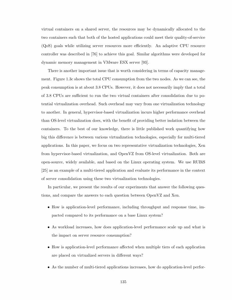
virtual containers on a shared server, the resources may be dynamically allocated to the
two containers such that both of the hosted applications could meet their quality-of-service
(QoS) goals while utilizing server resources more efficiently. An adaptive CPU resource
controller was described in [76] to achieve this goal. Similar algorithms were developed for
dynamic memory management in VMware ESX server [93].
There is another important issue that is worth considering in terms of capacity manage-
ment. Figure 1.3c shows the total CPU consumption from the two nodes. As we can see, the
peak consumption is at about 3.8 CPUs. However, it does not necessarily imply that a total
of 3.8 CPUs are sufficient to run the two virtual containers after consolidation due to po-
tential virtualization overhead. Such overhead may vary from one virtualization technology
to another. In general, hypervisor-based virtualization incurs higher performance overhead
than OS-level virtualization does, with the benefit of providing better isolation between the
containers. To the best of our knowledge, there is little published work quantifying how
big this difference is between various virtualization technologies, especially for multi-tiered
applications. In this paper, we focus on two representative virtualization technologies, Xen
from hypervisor-based virtualization, and OpenVZ from OS-level virtualization. Both are
open-source, widely available, and based on the Linux operating system. We use RUBiS
[25] as an example of a multi-tiered application and evaluate its performance in the context
of server consolidation using these two virtualization technologies.
In particular, we present the results of our experiments that answer the following ques-
tions, and compare the answers to each question between OpenVZ and Xen.
• How is application-level performance, including throughput and response time, im-
pacted compared to its performance on a base Linux system?
• As workload increases, how does application-level performance scale up and what is
the impact on server resource consumption?
• How is application-level performance affected when multiple tiers of each application
are placed on virtualized servers in different ways?
• As the number of multi-tiered applications increases, how do application-level perfor-
135
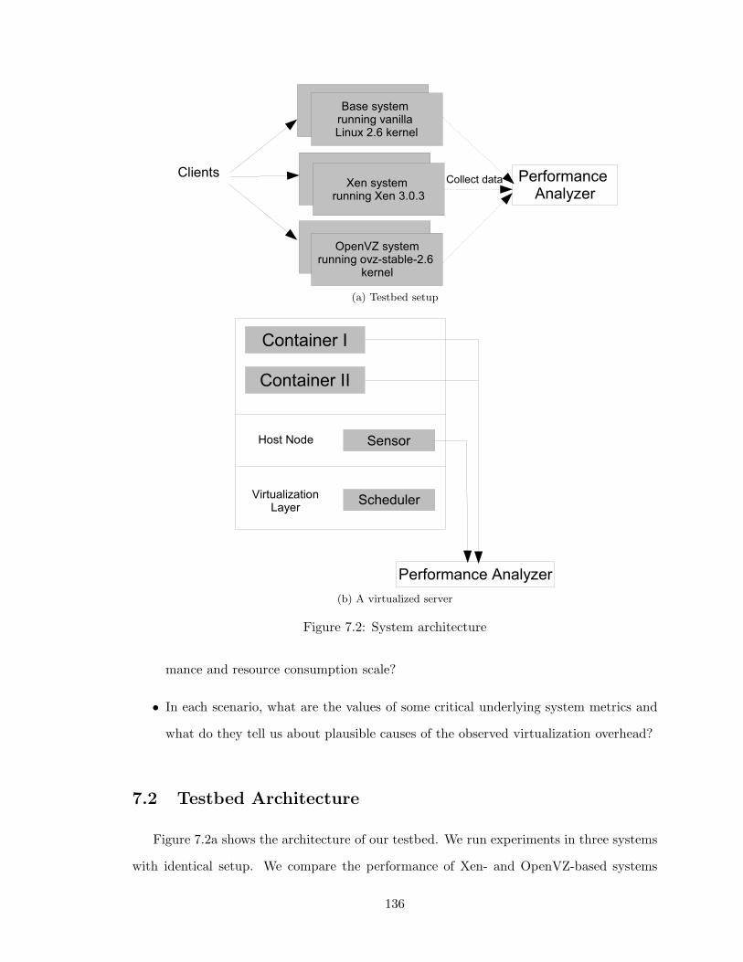
(a) Testbed setup
(b) A virtualized server
Figure 7.2: System architecture
mance and resource consumption scale?
• In each scenario, what are the values of some critical underlying system metrics and
what do they tell us about plausible causes of the observed virtualization overhead?
7.2 Testbed Architecture
Figure 7.2a shows the architecture of our testbed. We run experiments in three systems
with identical setup. We compare the performance of Xen- and OpenVZ-based systems
136
with that of a vanilla Linux system (referred to as base system here after). In a virtualized
configuration, each physical node may host one or more virtual containers supported by Xen
or OpenVZ as shown in Figure 7.2b. Because we are interested in multi-tiered applications,
two separate nodes may be used for the Web and the database tiers. Each node is equipped
with a sensor collecting various performance metrics including CPU consumption, memory
consumption and other performance events collected by Oprofile [7]. This data is collected
on a separate machine and analyzed later.
We use HP Proliant DL385 G1 for all our servers and client machines. Every server
has two 2.6 GHz processors, each with 1MB of L2 cache, 8 GB of RAM, and two Gigabit
network interfaces.
7.2.1 System Configurations
We conduct our experiments on three different systems as explained below. All systems
are carefully set up to be as similar as possible with the same amount of resources (memory
and CPU) allocated to a particular virtual container.
7.2.1.1 Base system
We use a plain vanilla 2.6 Linux kernel that comes with the Fedora Core 5 standard
distribution as our base system. Standard packages available from Fedora repository are
used to set up various applications.
7.2.1.2 Xen system
Xen is a paravirtualization [98] technology that allows multiple guest operating systems
to be run in virtual containers (called domains). The Xen hypervisor provides a thin
software virtualization layer between the guest OS and the underlying hardware. Each guest
OS is a modified version of the base Linux (XenLinux) because the hardware abstraction
presented by the hypervisor is similar but not identical to the raw hardware. The hypervisor
contains a CPU scheduler that implements various scheduling policies including proportional
fair-share, along with other modules such as the memory management unit.
137
We use the Xen 3.0.3 unstable branch [14] for our experiments as it provides a credit-
based CPU scheduler (in short, credit scheduler), which, in our experiments, provides better
performance than the earlier SEDF scheduler. The credit scheduler allows each domain to
be assigned a cap and a weight. A non-zero cap implements a non-work-conserving policy
for the CPU by specifying the maximum share of CPU time a domain can consume, even
if there exist idle CPU cycles. When the cap is zero, the scheduler switches to a work-
conserving mode, where weights for multiple domains determine their relative shares of
CPU time when the CPU is under contention. At the same time, a domain can use extra
CPU time beyond its share if other domains do not need it. In all our experiments, we
use the non-capped mode of the credit scheduler, and the system is compiled using the uni-
processor architecture. In this case, Dom0 and all the guest domains share the full capacity
of a single processor.
7.2.1.3 OpenVZ system
OpenVZ [6] is a Linux-based OS-level server virtualization technology. It allows creation
of secure, isolated virtual environments (VEs) on a single node enabling server consolidation.
Each VE performs and behaves exactly like a stand-alone server. They can be rebooted
independently and a different distribution with separate root directory can be set up. One
distinction between OpenVZ and Xen is that the former uses a single kernel shared by all
VEs. Therefore, it does not provide the same level of fault isolation as in the case of Xen.
In our experiments, we use the uni-processor version of OpenVZ stable 2.6 kernel that
provides a FSS scheduler, which also allows the CPU share of each VE to be either capped
or not capped. Similar to the Xen system, the non-capped option is used in the OpenVZ
system.
In the remainder of this paper, we use the term virtual container to refer to either a
domain in Xen or a VE in OpenVZ.
138

7.2.2 Instrumentation
To measure the CPU consumption accurately, we wrote scripts that use existing tools
to gather data. In the base system, the output from command top -b is gathered and then
analyzed later. Similarly, xentop -b is used in the Xen case, which provides information
on the CPU consumptions of individual domains. For OpenVZ, there is no existing tool to
directly measure the CPU consumption by a particular container. We use the data provided
from /proc/vz/vestat to measure the amount of CPU time spent by a particular VE.
7.2.2.1 Oprofile
Oprofile [7] is a tool for measuring certain hardware events using hardware performance
counters. For example, one can measure the number of cache misses that happen in a
particular application. The profiles generated by Oprofile are very detailed and can provide
a wealth of information. Menon et al. [67] have modified Oprofile to support Xen. The
resulting tool, Xenoprof, allows one to profile multiple domains in a Xen system. For each
set of experiments, we analyze the data generated by Oprofile and provide our insights on
the performance overheads.
We concentrate on two aspects when analyzing the data generated by Oprofile:
• Comparing hardware performance counters for various configurations;
• Understanding differences in overheads experienced within specific kernels. We want
to identify particular kernel sub-systems where most of the overhead occurs and quan-
tify it.
We monitor three hardware counters for our analysis:
• CPU_CLK_UNHALT: The number of cycles outside of halt state. It provides a rough
estimate of the CPU time used by a particular binary or a symbol.
• RETIRED_INSTRUCTIONS: The number of instructions that are retired. It is a rough
estimate of the number of instructions executed by a binary or a symbol.
• L2_CACHE_MISS: The number of L2 cache misses. It measures the number of times
the memory references in an instruction miss the L2 cache and access main memory.
139

DB
Web
Server
(a) Single-node
Server 1 Server 2
Web DB
(b) Two-node, one-instance
Server 1 Server 2
Web II
Web I DB I
DB II
(c) Two-node, two-instance
Server 1 Server 2
Web I DB I....
.
.
..
Web IV DB IV
(d) Two-node, four-instance
Figure 7.3: Various configurations for consolidation
We thoroughly analyze differences in these counter values in various configurations, and
infer sources of overhead in respective virtualization technologies.
7.3 Design of Experiments
The experiments are designed with the goal of quantitatively evaluating the impact of
virtualization on server consolidation. Specifically, we are not interested in performing mi-
cro benchmarks that compare the performance of system calls, page miss penalties, etc.
Instead, we focus more on how application-level performance, including throughput and re-
sponse time, are affected when using different virtualization technologies as well as different
configurations for consolidation.
Today’s enterprise applications typically employ a multi-tiered architecture, where the
Web and the application tiers serve static files and implement business logic, and the
database (DB) tier executes data queries and interacts with the storage devices. Dur-
ing server consolidation, the various tiers of an application that are traditionally hosted on
140
dedicated servers are moved onto shared servers. Moreover, when virtualization is involved,
each of these tiers is hosted in a virtual container, which can have performance implications
for the application.
We have chosen RUBiS [25], an online auction site benchmark, as an example of a multi-
tiered application. We use a version of the application that has a two-tier structure: the
Web tier contains an Apache Web server with PHP, and the DB tier uses a MySQL database
server. RUBiS clients connect to the Web tier and perform various operations simulating
auctions. Each client starts a session in which the client browses through items, looks at
prices, and buys or sells items. In each session, the client waits for a request to complete
before sending out the next request. If the request fails due to timed-outs, the session
is aborted and a new session is started. This gives rise to a closed-loop behavior where
the clients wait for the server when it is overloaded. Although RUBiS provides different
workload mixes, we use the browsing mix in our experiments, which introduces higher load
on the Web tier than on the DB tier.
We consider running RUBiS on consolidated servers. In addition to the comparison
between OpenVZ and Xen, we also need to understand how application performance is
impacted by different placement of application tiers on the consolidated servers. We evaluate
the following two configurations for consolidation.
• Single-node: Both the Web and the DB tiers of a single RUBiS application are
hosted on a single physical node (Figure 7.3a).
• Two-node: The Web and the DB tiers of a single RUBiS application are distributed
on two separate nodes (Figure 7.3b).
There are additional reasons why one configuration may be chosen over the other in
a practical scenario. For example, the single-node configuration may be chosen since it
reduces network traffic by hosting multiple tiers of the same application on a single server,
whereas the two-node option may be preferable in a case where it can reduce software
licensing cost. In this work, we only focus on application performance differences in the two
configurations and how performance scales as the workload increases.
141

80
90
100
110
120
130
140
500 550 600 650 700 750 800
Thr
ough
put (
reqs
/sec
)
Number of Threads
BaseXen
OpenVZ
(a) Throughput
0
20
40
60
80
100
120
140
500 550 600 650 700 750 800
Res
pons
e T
ime
(ms)
Number of Threads
BaseXen
OpenVZ
(b) Average response time
Figure 7.4: Single-node - application performance
In addition, we are also interested in scalability of the virtualized systems when the
number of applications hosted increases in the two-node case. Each node may host multiples
of the Web or the DB tier as shown in Figures 7.3c and 7.3d. In our experiments, we increase
the number of RUBiS instances from one to two and then to four, and compare OpenVZ
with Xen in application-level performance and system resource consumption. For each
scenario, we provide a detailed analysis of the corresponding Oprofile statistics and point
to plausible causes for the observed virtualization overheads.
7.4 Evaluation Results
This section reports the results of our experimental evaluation using the RUBiS bench-
mark. In particular, we compare two different configuration options, single-node vs. two-
node, for placing the two tiers of a single RUBiS application on physical servers. All
experiments are done on the base, OpenVZ, and Xen systems, and a three-way comparison
of the results is presented.
7.4.1 Single-node
In this configuration, both the Web and the DB tiers are hosted on a single node, as
shown in Figure 7.3a. In both the Xen and the OpenVZ systems, the two tiers run in two
separate virtual containers. To evaluate the performance of each system, we scale up the
142
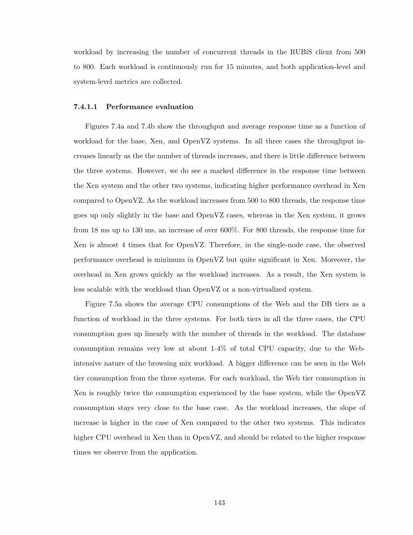
workload by increasing the number of concurrent threads in the RUBiS client from 500
to 800. Each workload is continuously run for 15 minutes, and both application-level and
system-level metrics are collected.
7.4.1.1 Performance evaluation
Figures 7.4a and 7.4b show the throughput and average response time as a function of
workload for the base, Xen, and OpenVZ systems. In all three cases the throughput in-
creases linearly as the the number of threads increases, and there is little difference between
the three systems. However, we do see a marked difference in the response time between
the Xen system and the other two systems, indicating higher performance overhead in Xen
compared to OpenVZ. As the workload increases from 500 to 800 threads, the response time
goes up only slightly in the base and OpenVZ cases, whereas in the Xen system, it grows
from 18 ms up to 130 ms, an increase of over 600%. For 800 threads, the response time for
Xen is almost 4 times that for OpenVZ. Therefore, in the single-node case, the observed
performance overhead is minimum in OpenVZ but quite significant in Xen. Moreover, the
overhead in Xen grows quickly as the workload increases. As a result, the Xen system is
less scalable with the workload than OpenVZ or a non-virtualized system.
Figure 7.5a shows the average CPU consumptions of the Web and the DB tiers as a
function of workload in the three systems. For both tiers in all the three cases, the CPU
consumption goes up linearly with the number of threads in the workload. The database
consumption remains very low at about 1-4% of total CPU capacity, due to the Web-
intensive nature of the browsing mix workload. A bigger difference can be seen in the Web
tier consumption from the three systems. For each workload, the Web tier consumption in
Xen is roughly twice the consumption experienced by the base system, while the OpenVZ
consumption stays very close to the base case. As the workload increases, the slope of
increase is higher in the case of Xen compared to the other two systems. This indicates
higher CPU overhead in Xen than in OpenVZ, and should be related to the higher response
times we observe from the application.
143
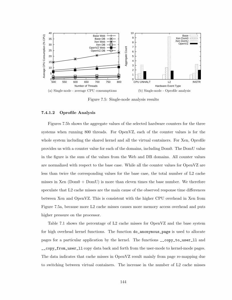
0
5
10
15
20
25
30
35
40
500 550 600 650 700 750 800
Ave
rage
CP
U C
onsu
mpt
ion
(% C
PU
)
Number of Threads
Base WebBase DBXen Web
Xen DBOpenVZ Web
OpenVZ DB
(a) Single-node - average CPU consumptions
0
1
2
3
4
5
6
7
8
9
10
INSTRL2CPU UNHALT
Agg
rega
te C
ount
Hardware Event Type
BaseXen Dom0Xen DomU
OpenVZ
(b) Single-node - Oprofile analysis
Figure 7.5: Single-node analysis results
7.4.1.2 Oprofile Analysis
Figures 7.5b shows the aggregate values of the selected hardware counters for the three
systems when running 800 threads. For OpenVZ, each of the counter values is for the
whole system including the shared kernel and all the virtual containers. For Xen, Oprofile
provides us with a counter value for each of the domains, including Dom0. The DomU value
in the figure is the sum of the values from the Web and DB domains. All counter values
are normalized with respect to the base case. While all the counter values for OpenVZ are
less than twice the corresponding values for the base case, the total number of L2 cache
misses in Xen (Dom0 + DomU) is more than eleven times the base number. We therefore
speculate that L2 cache misses are the main cause of the observed response time differences
between Xen and OpenVZ. This is consistent with the higher CPU overhead in Xen from
Figure 7.5a, because more L2 cache misses causes more memory access overhead and puts
higher pressure on the processor.
Table 7.1 shows the percentage of L2 cache misses for OpenVZ and the base system
for high overhead kernel functions. The function do_anonymous_page is used to allocate
pages for a particular application by the kernel. The functions __copy_to_user_ll and
__copy_from_user_ll copy data back and forth from the user-mode to kernel-mode pages.
The data indicates that cache misses in OpenVZ result mainly from page re-mapping due
to switching between virtual containers. The increase in the number of L2 cache misses
144

Symbol Name OpenVZ Base
do_anonymous_page 31.84 25.24__copy_to_user_ll 11.77 9.67__copy_from_user_ll 7.23 0.73
Table 7.1: Base vs OpenVZ - % of L2 cache misses
Symbol name L2 cache misses (%)
hypervisor_callback 32.00evtchn_do_upcall 44.54__copy_to_user_ll 3.57__do_IRQ 2.45
Table 7.2: Xen Web tier - % of L2 cache misses
causes the instructions to stall and reduces the total number of instructions executed.
Because Xen uses a modified kernel, it is not possible to directly compare calls within it
with the numbers obtained from the base system and OpenVZ. Table 7.2 shows the highest
cache miss functions identified using Oprofile for the Web domain in the Xen system.
The function hypervisor_callback is called when an event occurs that needs hyper-
visor attention. These events include various activities including cache misses, page faults,
and interrupt handling that usually happen in privileged mode in a normal kernel. After
some preliminary processing of stack frames, the function evtchn_do_upcall is called to
process the event and to set up the domain to continue normally. These functions are the
main source of overhead in Xen and reflect the cost of hypervisor-based virtualization.
Looking at the number of retired instructions for the Xen kernel (Table 7.3) for different
functions, we see that in addition to overheads in hypervisor callback and upcall event
handling, 10% of the instructions are executed to handle interrupts, which also is a major
source of overhead. The higher percentage is due to increase in the interrupts caused by
switching between the two domains.
We also looked at the hardware counters for a particular binary (like httpd, mysqld).
Symbol name Number of ret instr(%)
hypervisor_callback 39.61evtchn_do_upcall 7.53__do_IRQ 10.9l
Table 7.3: Xen kernel - % of retired instructions
145
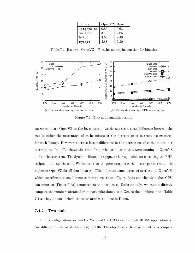
Binary OpenVZ Base
libphp5.so 0.85 0.63vmlinux 3.13 2.85httpd 4.56 2.40mysqld 4.88 2.30
Table 7.4: Base vs. OpenVZ - % cache misses/instruction for binaries
0
5
10
15
20
25
30
500 550 600 650 700 750 800
Res
pons
e T
ime
(ms)
Number of Threads
BaseXen
OpenVZ
(a) Two-node - average response time
0
5
10
15
20
25
30
35
40
500 550 600 650 700 750 800A
vera
ge C
PU
Con
sum
ptio
n (%
CP
U)
Number of Threads
Base WebBase DBXen Web
Xen DBOpenVZ Web
OpenVZ DB
(b) Two-node - average CPU consumption
Figure 7.6: Two-node analysis results
As we compare OpenVZ to the base system, we do not see a clear difference between the
two in either the percentage of cache misses or the percentage of instructions executed
for each binary. However, there is larger difference in the percentage of cache misses per
instruction. Table 7.4 shows this ratio for particular binaries that were running in OpenVZ
and the base system. The dynamic library libphp5.so is responsible for executing the PHP
scripts on the apache side. We can see that the percentage of cache misses per instruction is
higher in OpenVZ for all four binaries. This indicates some degree of overhead in OpenVZ,
which contributes to small increase in response times (Figure 7.4b) and slightly higher CPU
consumption (Figure 7.5a) compared to the base case. Unfortunately, we cannot directly
compare the numbers obtained from particular domains in Xen to the numbers in the Table
7.4 as they do not include the associated work done in Dom0.
7.4.2 Two-node
In this configuration, we run the Web and the DB tiers of a single RUBiS application on
two different nodes, as shown in Figure 7.3b. The objective of the experiment is to compare
146
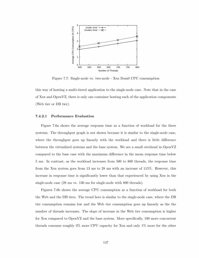
0
1
2
3
4
5
500 550 600 650 700 750 800
Ave
rage
CP
U C
onsu
mpt
ion
(% C
PU
)Number of Threads
1node 1inst2nodes 1inst
Figure 7.7: Single-node vs. two-node - Xen Dom0 CPU consumption
this way of hosting a multi-tiered application to the single-node case. Note that in the case
of Xen and OpenVZ, there is only one container hosting each of the application components
(Web tier or DB tier).
7.4.2.1 Performance Evaluation
Figure 7.6a shows the average response time as a function of workload for the three
systems. The throughput graph is not shown because it is similar to the single-node case,
where the throughput goes up linearly with the workload and there is little difference
between the virtualized systems and the base system. We see a small overhead in OpenVZ
compared to the base case with the maximum difference in the mean response time below
5 ms. In contrast, as the workload increases from 500 to 800 threads, the response time
from the Xen system goes from 13 ms to 28 ms with an increase of 115%. However, this
increase in response time is significantly lower than that experienced by using Xen in the
single-node case (28 ms vs. 130 ms for single-node with 800 threads).
Figures 7.6b shows the average CPU consumption as a function of workload for both
the Web and the DB tiers. The trend here is similar to the single-node case, where the DB
tier consumption remains low and the Web tier consumption goes up linearly as the the
number of threads increases. The slope of increase in the Web tier consumption is higher
for Xen compared to OpenVZ and the base system. More specifically, 100 more concurrent
threads consume roughly 3% more CPU capacity for Xen and only 1% more for the other
147
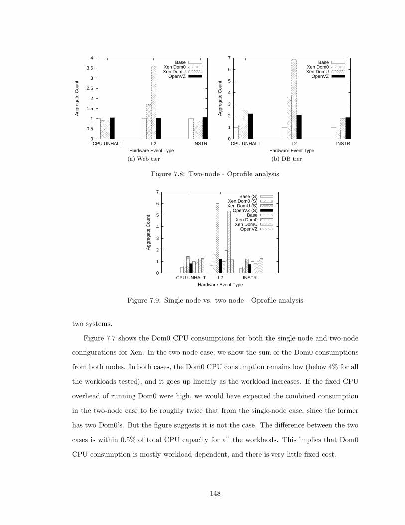
0
0.5
1
1.5
2
2.5
3
3.5
4
INSTRL2CPU UNHALT
Agg
rega
te C
ount
Hardware Event Type
BaseXen Dom0Xen DomU
OpenVZ
(a) Web tier
0
1
2
3
4
5
6
7
INSTRL2CPU UNHALT
Agg
rega
te C
ount
Hardware Event Type
BaseXen Dom0Xen DomU
OpenVZ
(b) DB tier
Figure 7.8: Two-node - Oprofile analysis
0
1
2
3
4
5
6
7
INSTRL2CPU UNHALT
Agg
rega
te C
ount
Hardware Event Type
Base (S)Xen Dom0 (S)Xen DomU (S)
OpenVZ (S)Base
Xen Dom0Xen DomU
OpenVZ
Figure 7.9: Single-node vs. two-node - Oprofile analysis
two systems.
Figure 7.7 shows the Dom0 CPU consumptions for both the single-node and two-node
configurations for Xen. In the two-node case, we show the sum of the Dom0 consumptions
from both nodes. In both cases, the Dom0 CPU consumption remains low (below 4% for all
the workloads tested), and it goes up linearly as the workload increases. If the fixed CPU
overhead of running Dom0 were high, we would have expected the combined consumption
in the two-node case to be roughly twice that from the single-node case, since the former
has two Dom0’s. But the figure suggests it is not the case. The difference between the two
cases is within 0.5% of total CPU capacity for all the worklaods. This implies that Dom0
CPU consumption is mostly workload dependent, and there is very little fixed cost.
148
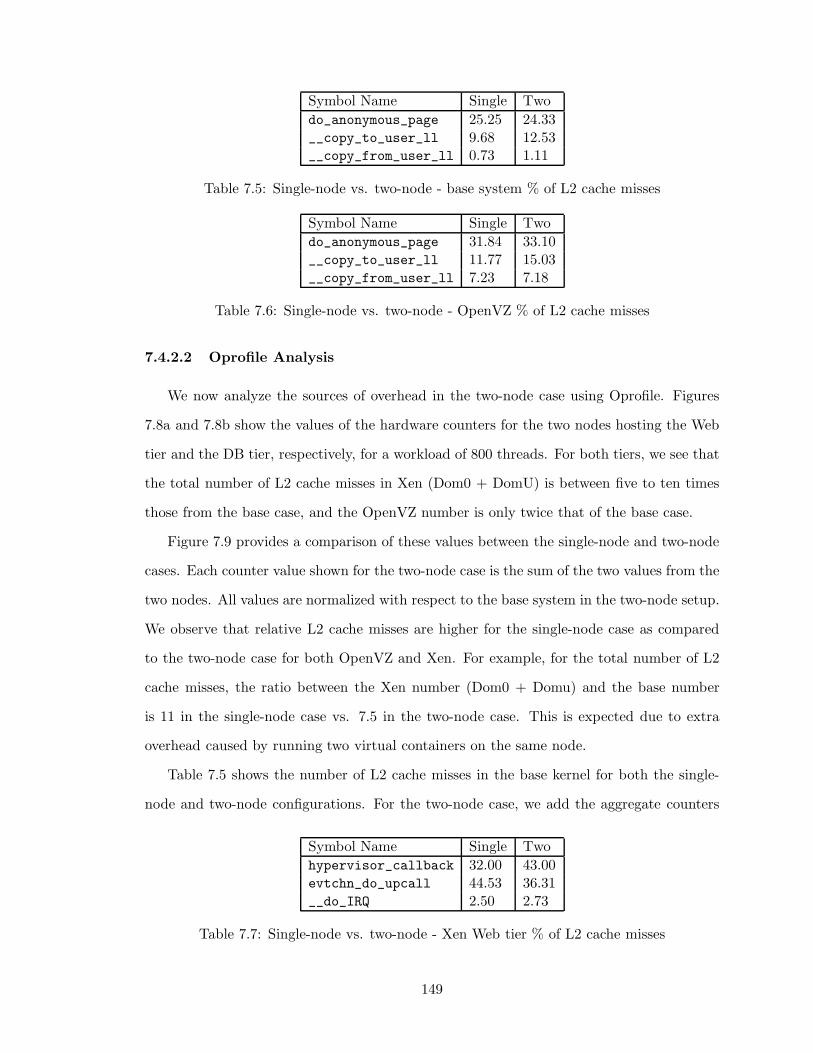
Symbol Name Single Two
do_anonymous_page 25.25 24.33__copy_to_user_ll 9.68 12.53__copy_from_user_ll 0.73 1.11
Table 7.5: Single-node vs. two-node - base system % of L2 cache misses
Symbol Name Single Two
do_anonymous_page 31.84 33.10__copy_to_user_ll 11.77 15.03__copy_from_user_ll 7.23 7.18
Table 7.6: Single-node vs. two-node - OpenVZ % of L2 cache misses
7.4.2.2 Oprofile Analysis
We now analyze the sources of overhead in the two-node case using Oprofile. Figures
7.8a and 7.8b show the values of the hardware counters for the two nodes hosting the Web
tier and the DB tier, respectively, for a workload of 800 threads. For both tiers, we see that
the total number of L2 cache misses in Xen (Dom0 + DomU) is between five to ten times
those from the base case, and the OpenVZ number is only twice that of the base case.
Figure 7.9 provides a comparison of these values between the single-node and two-node
cases. Each counter value shown for the two-node case is the sum of the two values from the
two nodes. All values are normalized with respect to the base system in the two-node setup.
We observe that relative L2 cache misses are higher for the single-node case as compared
to the two-node case for both OpenVZ and Xen. For example, for the total number of L2
cache misses, the ratio between the Xen number (Dom0 + Domu) and the base number
is 11 in the single-node case vs. 7.5 in the two-node case. This is expected due to extra
overhead caused by running two virtual containers on the same node.
Table 7.5 shows the number of L2 cache misses in the base kernel for both the single-
node and two-node configurations. For the two-node case, we add the aggregate counters
Symbol Name Single Two
hypervisor_callback 32.00 43.00evtchn_do_upcall 44.53 36.31__do_IRQ 2.50 2.73
Table 7.7: Single-node vs. two-node - Xen Web tier % of L2 cache misses
149

Symbol Name Single Two
hypervisor_callback 6.10 4.15evtchn_do_upcall 44.21 42.42__do_IRQ 1.73 1.21
Table 7.8: Single-node vs. two-node - Xen Web tier % of L2 cache misses/instruction
for each kernel function in both nodes and normalize them with respect to the total number
of cache misses from the two nodes. The same comparison is shown in Table 7.6 for the
OpenVZ system. The percentage of L2 cache misses for different kernel functions stay
almost the same between the single-node and two-node cases (within 4% of each other),
except for the __copy_to_user_ll function where we see the two-node value being 28%
higher. Comparing Table 7.6 to Table 7.5, we see that all the values are higher in OpenVZ
than in the base case indicating higher page re-mapping overhead in the OpenVZ system.
Table 7.7 shows a similar comparison for Xen-specific kernel calls in the Xen system
Web tier. If we add the first two rows, we see that the total number of cache misses for the
functions hypervisor_call_back and evtchn_do_upcall is very similar in the single-node
and two-node cases. The values for the _do_IRQ call are similar too. However, the difference
is larger in the number of cache misses per instruction, which is shown in Table 7.8. We see
the sum of the first two rows being 10% higher in the single-node case, and the percentage
of L2 cache misses/instruction for interrupt handling being 43% higher. The reason is that
more instructions are executed in the two-node case because of less stalling due to cache
misses.
7.5 Scalability Evaluation
In this section, we investigate the scale of consolidation that can be achieved by different
virtualization technologies. We increase the number of RUBiS instances from one to two
then to four in the two-node configuration, and compare the scalability of Xen and OpenVZ
with respect to application performance and resource consumption.
150
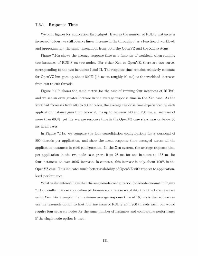
7.5.1 Response Time
We omit figures for application throughput. Even as the number of RUBiS instances is
increased to four, we still observe linear increase in the throughput as a function of workload,
and approximately the same throughput from both the OpenVZ and the Xen systems.
Figure 7.10a shows the average response time as a function of workload when running
two instances of RUBiS on two nodes. For either Xen or OpenVZ, there are two curves
corresponding to the two instances I and II. The response time remains relatively constant
for OpenVZ but goes up about 500% (15 ms to roughly 90 ms) as the workload increases
from 500 to 800 threads.
Figure 7.10b shows the same metric for the case of running four instances of RUBiS,
and we see an even greater increase in the average response time in the Xen case. As the
workload increases from 500 to 800 threads, the average response time experienced by each
application instance goes from below 20 ms up to between 140 and 200 ms, an increase of
more than 600%, yet the average response time in the OpenVZ case stays near or below 30
ms in all cases.
In Figure 7.11a, we compare the four consolidation configurations for a workload of
800 threads per application, and show the mean response time averaged across all the
application instances in each configuration. In the Xen system, the average response time
per application in the two-node case grows from 28 ms for one instance to 158 ms for
four instances, an over 400% increase. In contrast, this increase is only about 100% in the
OpenVZ case. This indicates much better scalability of OpenVZ with respect to application-
level performance.
What is also interesting is that the single-node configuration (one-node one-inst in Figure
7.11a) results in worse application performance and worse scalability than the two-node case
using Xen. For example, if a maximum average response time of 160 ms is desired, we can
use the two-node option to host four instances of RUBiS with 800 threads each, but would
require four separate nodes for the same number of instances and comparable performance
if the single-node option is used.
151

0
10
20
30
40
50
60
70
80
90
100
400 500 600 700 800 900 1000 1100
Ave
rage
Res
pons
e T
ime
(ms)
Number of Threads
Xen IXen II
OpenVZ IOpenVZ II
(a) Two instances
0
20
40
60
80
100
120
140
160
180
200
400 500 600 700 800 900 1000 1100
Ave
rage
Res
pons
e T
ime
(ms)
Number of Threads
Xen IXen IIXen IIIXen IV
OpenVZ IOpenVZ IIOpenVZ IIIOpenVZ IV
(b) Four instances
Figure 7.10: two-node multiple instances - average response time
0
20
40
60
80
100
120
140
160
OpenVZXen
Res
pons
e tim
e (m
s)
System type
1node 1inst2node 1inst2node 2inst2node 4inst
(a) Average response time
0
5
10
15
20
25
30
OpenVZXen
Ave
rage
CP
U c
onsu
mpt
ion
(% C
PU
)
System type
1node 1inst2node 1inst2node 2inst2node 4inst
(b) Web tier CPU consumptions
Figure 7.11: Comparison of all configurations (800 threads)
0
2
4
6
8
10
12
500 550 600 650 700 750 800
Ave
rage
CP
U C
onsu
mpt
ion
(% C
PU
)
Number of Threads
2node 1inst 2node 2inst2node 4inst
Figure 7.12: two-node multiple instances - Xen Dom0 CPU consumption
152
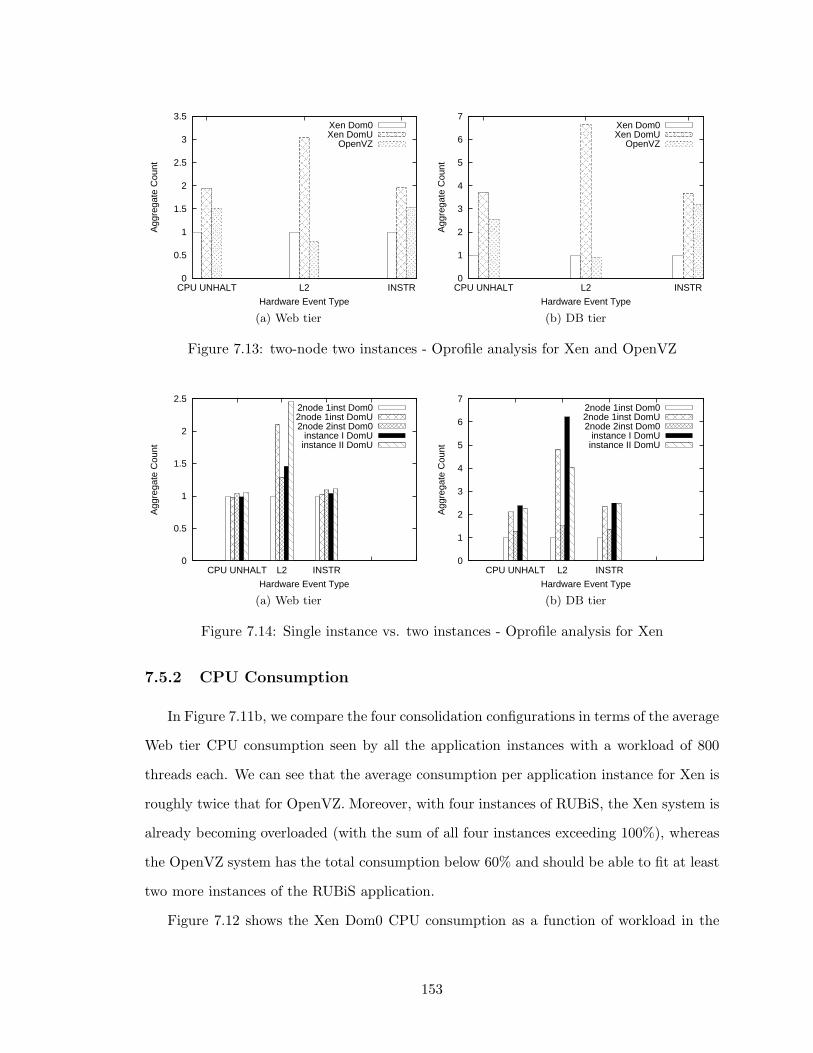
0
0.5
1
1.5
2
2.5
3
3.5
INSTRL2CPU UNHALT
Agg
rega
te C
ount
Hardware Event Type
Xen Dom0Xen DomU
OpenVZ
(a) Web tier
0
1
2
3
4
5
6
7
INSTRL2CPU UNHALT
Agg
rega
te C
ount
Hardware Event Type
Xen Dom0Xen DomU
OpenVZ
(b) DB tier
Figure 7.13: two-node two instances - Oprofile analysis for Xen and OpenVZ
0
0.5
1
1.5
2
2.5
INSTRL2CPU UNHALT
Agg
rega
te C
ount
Hardware Event Type
2node 1inst Dom02node 1inst DomU2node 2inst Dom0
instance I DomUinstance II DomU
(a) Web tier
0
1
2
3
4
5
6
7
INSTRL2CPU UNHALT
Agg
rega
te C
ount
Hardware Event Type
2node 1inst Dom02node 1inst DomU2node 2inst Dom0
instance I DomUinstance II DomU
(b) DB tier
Figure 7.14: Single instance vs. two instances - Oprofile analysis for Xen
7.5.2 CPU Consumption
In Figure 7.11b, we compare the four consolidation configurations in terms of the average
Web tier CPU consumption seen by all the application instances with a workload of 800
threads each. We can see that the average consumption per application instance for Xen is
roughly twice that for OpenVZ. Moreover, with four instances of RUBiS, the Xen system is
already becoming overloaded (with the sum of all four instances exceeding 100%), whereas
the OpenVZ system has the total consumption below 60% and should be able to fit at least
two more instances of the RUBiS application.
Figure 7.12 shows the Xen Dom0 CPU consumption as a function of workload in the
153
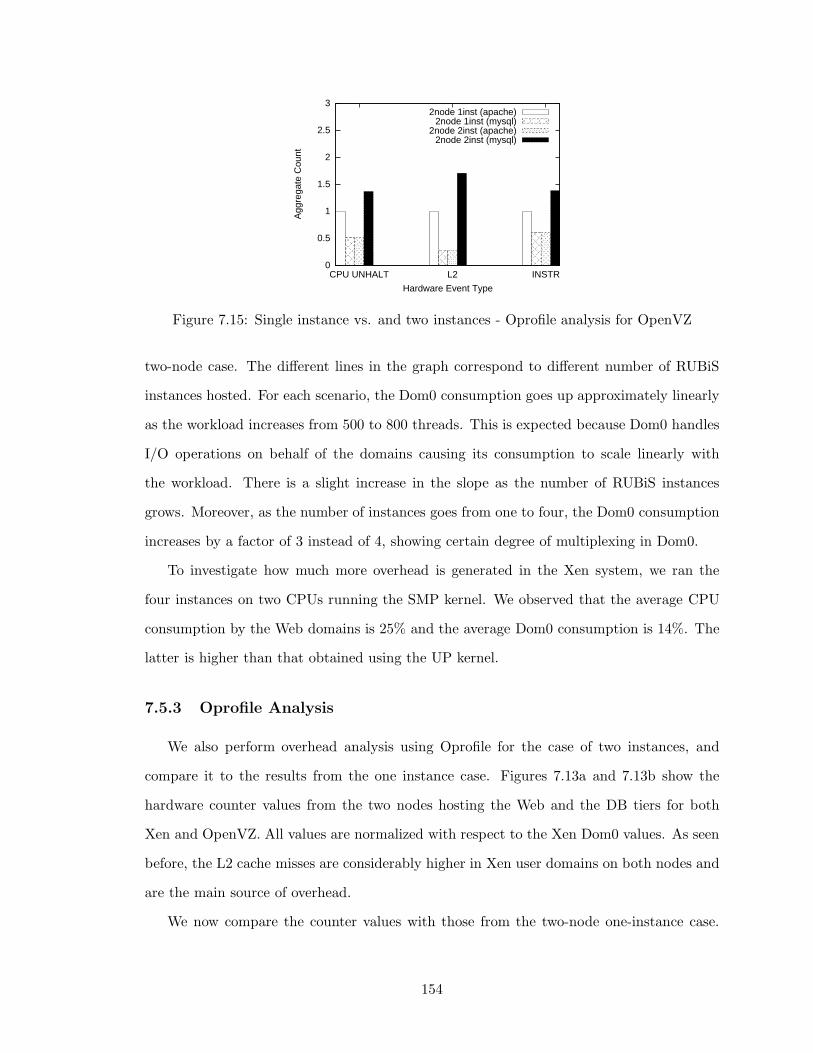
0
0.5
1
1.5
2
2.5
3
INSTRL2CPU UNHALT
Agg
rega
te C
ount
Hardware Event Type
2node 1inst (apache)2node 1inst (mysql)
2node 2inst (apache)2node 2inst (mysql)
Figure 7.15: Single instance vs. and two instances - Oprofile analysis for OpenVZ
two-node case. The different lines in the graph correspond to different number of RUBiS
instances hosted. For each scenario, the Dom0 consumption goes up approximately linearly
as the workload increases from 500 to 800 threads. This is expected because Dom0 handles
I/O operations on behalf of the domains causing its consumption to scale linearly with
the workload. There is a slight increase in the slope as the number of RUBiS instances
grows. Moreover, as the number of instances goes from one to four, the Dom0 consumption
increases by a factor of 3 instead of 4, showing certain degree of multiplexing in Dom0.
To investigate how much more overhead is generated in the Xen system, we ran the
four instances on two CPUs running the SMP kernel. We observed that the average CPU
consumption by the Web domains is 25% and the average Dom0 consumption is 14%. The
latter is higher than that obtained using the UP kernel.
7.5.3 Oprofile Analysis
We also perform overhead analysis using Oprofile for the case of two instances, and
compare it to the results from the one instance case. Figures 7.13a and 7.13b show the
hardware counter values from the two nodes hosting the Web and the DB tiers for both
Xen and OpenVZ. All values are normalized with respect to the Xen Dom0 values. As seen
before, the L2 cache misses are considerably higher in Xen user domains on both nodes and
are the main source of overhead.
We now compare the counter values with those from the two-node one-instance case.
154
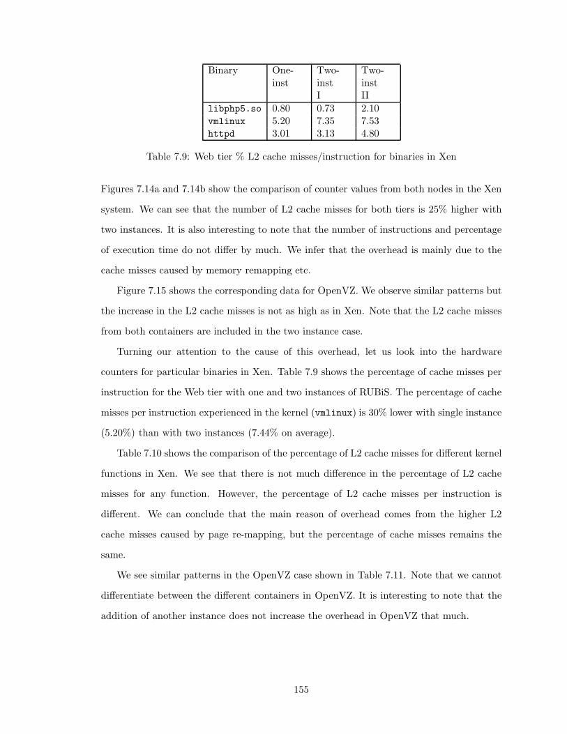
Binary One-inst
Two-instI
Two-instII
libphp5.so 0.80 0.73 2.10vmlinux 5.20 7.35 7.53httpd 3.01 3.13 4.80
Table 7.9: Web tier % L2 cache misses/instruction for binaries in Xen
Figures 7.14a and 7.14b show the comparison of counter values from both nodes in the Xen
system. We can see that the number of L2 cache misses for both tiers is 25% higher with
two instances. It is also interesting to note that the number of instructions and percentage
of execution time do not differ by much. We infer that the overhead is mainly due to the
cache misses caused by memory remapping etc.
Figure 7.15 shows the corresponding data for OpenVZ. We observe similar patterns but
the increase in the L2 cache misses is not as high as in Xen. Note that the L2 cache misses
from both containers are included in the two instance case.
Turning our attention to the cause of this overhead, let us look into the hardware
counters for particular binaries in Xen. Table 7.9 shows the percentage of cache misses per
instruction for the Web tier with one and two instances of RUBiS. The percentage of cache
misses per instruction experienced in the kernel (vmlinux) is 30% lower with single instance
(5.20%) than with two instances (7.44% on average).
Table 7.10 shows the comparison of the percentage of L2 cache misses for different kernel
functions in Xen. We see that there is not much difference in the percentage of L2 cache
misses for any function. However, the percentage of L2 cache misses per instruction is
different. We can conclude that the main reason of overhead comes from the higher L2
cache misses caused by page re-mapping, but the percentage of cache misses remains the
same.
We see similar patterns in the OpenVZ case shown in Table 7.11. Note that we cannot
differentiate between the different containers in OpenVZ. It is interesting to note that the
addition of another instance does not increase the overhead in OpenVZ that much.
155
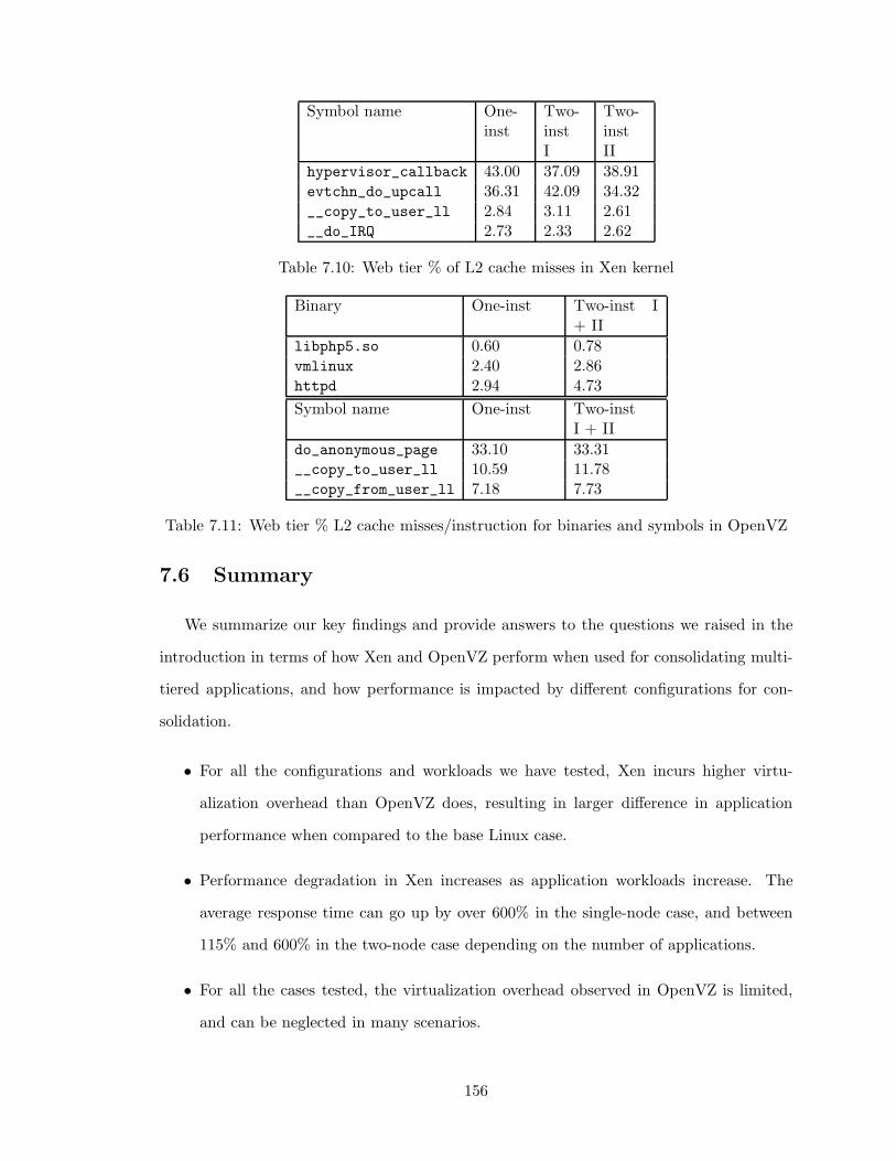
Symbol name One-inst
Two-instI
Two-instII
hypervisor_callback 43.00 37.09 38.91evtchn_do_upcall 36.31 42.09 34.32__copy_to_user_ll 2.84 3.11 2.61__do_IRQ 2.73 2.33 2.62
Table 7.10: Web tier % of L2 cache misses in Xen kernel
Binary One-inst Two-inst I+ II
libphp5.so 0.60 0.78vmlinux 2.40 2.86httpd 2.94 4.73
Symbol name One-inst Two-instI + II
do_anonymous_page 33.10 33.31__copy_to_user_ll 10.59 11.78__copy_from_user_ll 7.18 7.73
Table 7.11: Web tier % L2 cache misses/instruction for binaries and symbols in OpenVZ
7.6 Summary
We summarize our key findings and provide answers to the questions we raised in the
introduction in terms of how Xen and OpenVZ perform when used for consolidating multi-
tiered applications, and how performance is impacted by different configurations for con-
solidation.
• For all the configurations and workloads we have tested, Xen incurs higher virtu-
alization overhead than OpenVZ does, resulting in larger difference in application
performance when compared to the base Linux case.
• Performance degradation in Xen increases as application workloads increase. The
average response time can go up by over 600% in the single-node case, and between
115% and 600% in the two-node case depending on the number of applications.
• For all the cases tested, the virtualization overhead observed in OpenVZ is limited,
and can be neglected in many scenarios.
156

• For all configurations, the Web tier CPU consumption for Xen is roughly twice that
of the base system or OpenVZ. CPU consumption of all systems and all containers
goes up linearly as the workload increases. The slope of increase in the case of Xen is
higher than in OpenVZ and the base cases.
• The main cause of performance overhead in Xen is the number of L2 cache misses.
• In the Xen system, relative L2 cache misses are higher in the single-node case compared
to the sum of cache misses in the two-node case. Between the base and OpenVZ
systems, the difference is minor.
• In the Xen system, the percentage of L2 cache misses for a particular function in the
kernel is similar in the single-node and two-node cases. But the percentage of misses
per instruction is higher in the single-node case.
• The percentage increase in the number of L2 cache misses for single and multiple
instances of RUBiS is higher in Xen than in OpenVZ. In other words, as the number
of applications increases, OpenVZ scales with less overhead.
• In the Xen system in a two-node setup, the percentage increase in response time
from single application instance to multiple instances is significant (over 400% for 800
threads per application) while in OpenVZ this increase is much smaller (100%). With
our system setup in the two-node case, the Xen system becomes overloaded when
hosting four instances of RUBiS, while the OpenVZ system should be able to host at
least six without being overloaded.
• Hosting multiple tiers of a single application on the same node is not an efficient
solution compared to the case of hosting them on different nodes as far as response
time and CPU consumption are concerned.
In summary, there are many complex issues involved in consolidating servers running
enterprise applications using virtual containers. In this paper, we evaluated different ways
of consolidating multi-tiered systems using Xen and OpenVZ as virtualization technologies
and provided quantitative analysis to understand the differences in performance overheads.
157

More work can be done in extending this evaluation for various other complex enterprise
applications, including applications with higher memory requirements or database-intensive
applications. We hope that systems researchers can use these findings to develop opti-
mizations in virtualization technologies in the future to make them more suited for server
consolidation.
158
CHAPTER 8
Conclusions and Future Work
Virtualized data centers have seen explosive growth in recent years, but managing them
is still a hard problem. The main objective of this thesis is to automate the management
of a virtualized data center to achieve SLOs.
To that end, we have designed and implemented a set of tools that allow dynamic
allocation of resources to meet application SLOs.
We presented AutoControl, a feedback control system to dynamically allocate resources
to applications running on shared virtualized infrastructure. It consists of an online model
estimator that captures the dynamic relationship between application-level performance and
resource allocations and a MIMO resource controller that determines appropriate allocations
of multiple resources to achieve application-level SLOs.
We evaluated AutoControl using two testbeds consisting of varying numbers of Xen vir-
tual machines and various single- and multi-tier applications and benchmarks. Our experi-
mental results confirmed that AutoControl can detect dynamically-changing CPU and disk
bottlenecks across multiple nodes and can adjust resource allocations accordingly to achieve
end-to-end application-level SLOs. In addition, AutoControl can cope with dynamically-
shifting resource bottlenecks and provide service differentiation according to the priorities of
individual applications. Finally, we showed that AutoControl can enforce performance tar-
gets for different application-level metrics, including throughput and response time, under
dynamically-varying resource demands.
We have also built LiteGreen, an automated tool for saving desktop energy through
159

server consolidation. LiteGreen uses virtualization to resolve the problem of wasting energy,
by migrating idle desktops to a server where they can remain “always on” without incurring
the energy cost of a desktop machine. The seamlessness offered by LiteGreen allows us to
aggressively exploit short idle periods as well as long periods. Data-driven analysis of more
than 65000 hours of desktop usage traces from 120 users shows that LiteGreen can help
desktops sleep for 72-86% of the time and also scales well. The experience from our small-
scale deployment of LiteGreen has also been encouraging.
8.1 Limitations and Discussion
8.1.1 AutoControl
8.1.1.1 Limitations of control theory
Control theory provides a rich body of theory for building sound feedback systems.
However, applying control theory to computing systems is neither easy nor perfect.
1. Inherent non-linearity: Computer systems are inherently non-linear, making mod-
eling difficult. Unlike the classical linear control theory that is more intuitive and
accessible to people outside the field of control, nonlinear control theory and adaptive
control theory are much harder to understand and to apply in practice. Adaptive
control also imposes limitation on how fast workloads or system behavior can change.
2. Lack of first-principle models: Computer systems lack first-principle models, mak-
ing it necessary to build black box models. However, this approach requires controlled
experiments. Existing data collected from production systems are hard to use for
modeling purposes because it often lacks sufficient excitation to identify all relevant
correlations. It is difficult to design a set of controlled experiments to build a model
offline. An adaptive model may solve the problem, but will be more difficult to reason
about.
3. Tracking vs. Optimization: Most classical control problems are formulated as
tracking problems, i.e., the controller maintains the outputs at certain reference values.
160
However, this may not be appropriate for all design problems in systems. For example,
a meaningful design objective for a Web server may be to minimize the mean or
percentage response time instead of keeping it at a certain value. For such problems,
design methodologies that provide stability guarantees are not generally available.
4. Dealing with discrete inputs: Classical control theory only deals with continuous
inputs. Many computing systems have input variables that only take on discrete
values that have boundaries. For the systems where input values are discrete and
numerical (e.g., number of servers allocated or P-states in a processor with dynamic
voltage scaling enabled), it is possible to design controllers assuming continuous input
variables. This approach may suffer from instability or inefficiency due to quantization
errors. For systems with input values that are logical (e.g., Linux kernel version),
discrete-event control theory [35] can be explored.
8.1.1.2 Actuator & sensor behavior
The behavior of sensors and actuators affects our control. In existing systems, most
sensors return accurate information, but many actuators are poorly designed. We observed
various inaccuracies with Xen’s earlier SEDF scheduler and credit scheduler that are iden-
tified by other researchers [49] as well. These inaccuracies cause VMs to gain more or less
CPU than set by the controller. Empirical evidence shows that our controller is robust to
CPU scheduler’s inaccuracies.
8.1.1.3 Open Loop vs. Closed Loop Workloads
We have used closed loop workloads in our evaluation of AutoControl, but the Auto-
Control framework can work with open loop workloads as well without any modifications.
We treat the workload as a disturbance in the system that is external to the system, as a
result it does not matter how the workload behaves. As long as we can measure application
performance, the controller can use the adaptive online model to allocate the resources.
161

8.1.2 LiteGreen
The design of LiteGreen anticipates advances in virtualization technology that have
been reported in the literature and can reasonably be expected to become mainstream in
the not-too-distant future.
8.1.2.1 Memory ballooning and sharing challenges
Consolidation of multiple VMs on the same physical server can put pressure on the the
server’s memory resources. Page sharing is a technique to decrease the memory footprint
of VMs by sharing pages that are in common across multiple VMs [93]. Recent work [51]
has advanced the state-of-the-art to also include sub-page level sharing, yielding memory
savings of up to 90% with homogeneous VMs and up to 65% otherwise.
Even with page sharing, memory can become a bottleneck depending on the number of
VMs that are consolidated on the server. Memory ballooning is a technique to dynamically
shrink or grow the memory available to a VM with minimal overhead relative to stati-
cally provisioning the VM with the desired amount of memory [93]. Advances in memory
ballooning will help in LiteGreen consolidation.
8.1.2.2 Shared storage in live migration
Live migration assumes that the disk is shared between the source and destination
machines, say, in the form of network attached storage (NAS) on the LAN. This avoids
the considerable cost of migrating disk content. However, recent work has demonstrated
the migration of VMs with local virtual hard disks (VHDs) by using techniques such as
pre-copying and mirroring of disk content [32] to keep the downtime to under 3 seconds in
a LAN setting.
8.1.2.3 Desktop hypervisors
While much attention has been focused on server hypervisors, there has recently been
significant interest in client hypervisors, introducing challenges such as compatibility with
a diversity of devices and ensuring good graphics performance. In early 2009, both Citrix
162
and VMWare announced plans to build type-1 client hypervisors in collaboration with
Intel [18, 20].
While our prototype is constrained by the virtualization technology available to us today,
we believe that LiteGreen makes a contribution that is orthogonal to the advances noted
above.
8.1.3 Energy Proportional Systems
A fundamental assumption in LiteGreen is that the current desktop systems are not
energy proportional, as a result wasting great amount of energy, even when the system is
largely idle. There have been research advances in building energy proportional systems
[79, 80], and achieving energy proportionality with existing systems [89]. But, there is still
a long way to go before energy proportionality can be achieved. When energy proportional
systems are available, there is no need for LiteGreen.
8.1.4 Idleness Indicactors
In this thesis, we have used UI activity and CPU resource utiliaztion as an indicator for
measuring the idleness. However, these are only proxies for real user interactivity. Other
measures like network, disk activity, video display activity can be used to more accurately
determine the idleness. Other sensing based on location can be used to determine user’s
interactivity. Applying LiteGreen to use other indicators is left to future work.
8.2 Future Work
8.2.1 Network and Memory control
Our initial efforts in adding network resource control have failed, because of inaccuracies
in network actuators. Since Xen’s native network control is not fully implemented, we tried
to use Linux’s existing traffic controller (tc) to allocate network resources to VMs. We
found that the network bandwidth setting in (tc) is not enforced correctly when heavy
network workloads are run. We plan to fix these problems and add network control as well.
The MIMO resource controller, we developed in this thesis is directly applicable to any
163
number of resources.
The memory ballooning supported in VMware [93] provides a way of controlling the
memory required by a VM. However, the ballooning algorithm does not know about appli-
cation goals or multiple tiers, and only uses the memory pressure as seen by the operating
system. We have done preliminary work [54] in controlling CPU and memory together and
plan to integrate it with AutoControl.
8.2.2 Handling a Combination of Multiple Targets
AutoControl is shown to be able to handle different metrics, including throughput and
response time as performance metrics. How do we handle applications that require specifying
a combination of metrics for performance? For example, a web application might want to
specify certain maximum response time and minimum throughput goal. We have developed
a preliminary utility-based framework, where we introduce the concept of utility that is
a representative “value” of an application. For example, a utility function like U(y) =
max[α(1 − ey−yref , 0)] represents higher utility for an application as it reaches its target
metric yref . Continuing this, we can create a utility function using two or more metrics
that are of interest to the application. An example utility function using both response
time and throughput is: U(thr, rt) = g(rt − rtref + f(thrref − thr)), where g(x) = (1 +
erf(α ∗ x))/2 f(x) = β ∗ g(x).
A 3-D visualization of the function is shown in Figure 8.1.
8.2.3 Extending AutoControl to other applications
AutoControl is designed with allocating resources to single and multi-tier applications.
However, the modeling framework can be extended to other applications where individual
components can be modeled. This requires more support from the applicaiton, as Auto-
Control requires knobs to adjust resources for each of the components.
In this thesis, we have also assumed that we can identify the dependencies that can be
modeled explicitly. We assumed that in a 3-tier application, the dependency chain goes
from web server to application server to database server. However, this may not always
164
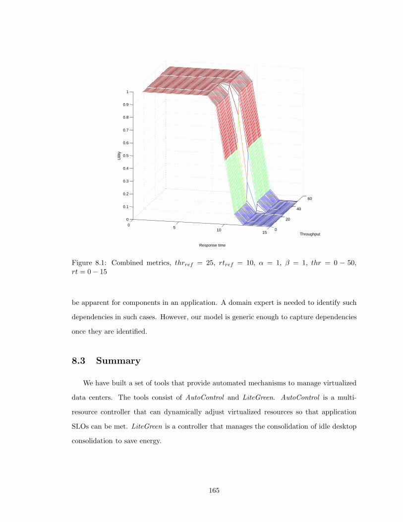
05
1015
0
20
40
60
0
0.1
0.2
0.3
0.4
0.5
0.6
0.7
0.8
0.9
1
Throughput
Response time
Uili
ty
Figure 8.1: Combined metrics, thrref = 25, rtref = 10, α = 1, β = 1, thr = 0 − 50,rt = 0− 15
be apparent for components in an application. A domain expert is needed to identify such
dependencies in such cases. However, our model is generic enough to capture dependencies
once they are identified.
8.3 Summary
We have built a set of tools that provide automated mechanisms to manage virtualized
data centers. The tools consist of AutoControl and LiteGreen. AutoControl is a multi-
resource controller that can dynamically adjust virtualized resources so that application
SLOs can be met. LiteGreen is a controller that manages the consolidation of idle desktop
consolidation to save energy.
165

BIBLIOGRAPHY
166

BIBLIOGRAPHY
[1] Amazon EC2: http://www.amazon.com/gp/browse.html ?node=201590011. http:
//www.amazon.com/gp/browse.html?node=201590011.
[2] Linux VServer, http://linux-vserver.org/. http://linux-vserver.org/.
[3] LiteGreen demo video. http://research.microsoft.com/en-us/projects/
litegreen/default.aspx.
[4] Microsoft Hyper-V. http://www.microsoft.com/windowsserver2008/en/us/
hyperv-main.aspx.
[5] Microsoft Virtual Server, http://www.microsoft. com/windowsserversystem/virtualserver/.http://www.microsoft.com/windowsserversystem/virtualserver/.
[6] OpenVZ: http://en.wikipedia.org/wiki/OpenVZ. http://en.wikipedia.org/wiki/OpenVZ.
[7] Oprofile: A system profiler for Linux, http://oprofile.sourceforge.net/. http://
oprofile.sourceforge.net/.
[8] Remote Desktop Protocol. http://msdn.microsoft.com/en-us/library/
aa383015(VS.85).aspx.
[9] Virtual Box. http://www.virtualbox.org/.
[10] Virtuozzo. http://www.parallels.com/products/virtuozzo/.
[11] VMWare ESX Server. http://www.vmware.com/products/esx/.
[12] Wattsup Meter. http://www.wattsupmeters.com.
[13] Windows Management Instrumentation. http://msdn.microsoft.com/en-us/
library/aa394582(VS.85).aspx.
[14] XenSource, http://www.xensource.com/. http://www.xensource.com/.
[15] White Paper: Benefits and Savings of Using Thin Clients, 2X Software Ltd., 2005.http://www.2x.com/whitepapers/WPthinclient.pdf.
[16] White Paper: Wake on LAN Technology, June 2006. http://www.liebsoft.com/
pdfs/Wake_On_LAN.pdf.
[17] Advanced Configuration and Power Interface (ACPI) Specification, June 2009. http://www.acpi.info/DOWNLOADS/ACPIspec40.pdf.
167
[18] Citrix XenClient Announcement, Jan. 2009. http://www.citrix.com/site/
resources/dynamic/partnerDocs/CitrixXenClient_SolutionBrief_Sept09.pdf.
[19] Emerging Technology Analysis: Hosted Virtual Desktops, Gartner, Feb. 2009. http://www.gartner.com/DisplayDocument?id=887912.
[20] VMWare Client Virtualization Platform (CVP) Announcement, Feb. 2009. http:
//www.vmware.com/company/news/releases/cvp-intel-vmworld.html.
[21] Worldwide PC 20092013 Forecast, IDC, Mar. 2009. http://idc.com/getdoc.jsp?
containerId=217360.
[22] Abdelzaher, T., Shin, K., and Bhatti, N. Performance guarantees for Webserver end-systems: A control-theoretical approach. IEEE Transactions on Paralleland Distributed Systems 13, 1 (2002).
[23] Agarwal, Y., Hodges, S., Chandra, R., Scott, J., Bahl, P., and Gupta, R.
Somniloquy: Augmenting Network Interfaces to Reduce PC Energy Usage. In NSDI(Apr. 2009).
[24] Agency, U. E. P. Report to Congress on Server and Data Center Energy EfficiencyPublic Law 109-431, Aug. 2007. \url{http://www.energystar.gov/ia/partners/
prod_development/downloads/EPA_Datacenter_Report_Congress_Final1.pdf}.
[25] Amza, C., Chanda, A., Cox, A., Elnikety, S., Gil, R., Rajamani, K., Cec-
chet, E., and Marguerite, J. Specification and implementation of dynamic Website benchmarks. In Proceedings of the 5th IEEE Annual Workshop on WorkloadCharacterization (Oct. 2002).
[26] Andrzejak, A., Arlitt, M., and Rolia, J. Bounding the resource sav-ings of utility computing models. Tech. Rep. HPL-2002-339, HP Labs, Dec.2002. http://www.hpl.hp.com/techreports/2002/HPL-2002-339.html;http://
www.hpl.hp.com/techreports/2002/HPL-2002-339.pdf.
[27] Aron, M., Druschel, P., and Zwaenepoel, W. Cluster reserves: A mechanismfor resource management in cluster-based network servers. In Proceedings of ACMSIGMETRICS (2000), pp. 90–101.
[28] Astrom, K., and Wittenmark, B. Adaptive Control. Addition-Wesley, 1995.
[29] Banga, G., Druschel, P., and Mogul, J. Resource containers: A new facilityfor resource management in server systems. In Proceedings of the 3rd Symposium onOperating Systems Design and Implementation (OSDI) (1999), pp. 45–58.
[30] Barham, P., Dragovic, B., Fraser, K., Hand, S., Harris, T., Ho, A.,
Neugebauer, R., Pratt, I., and Warfield, A. Xen and the art of virtualiza-tion. In Proceedings of the 19th symposium on Operating systems principles (SOSP)(New York, Oct. 19–22 2003), vol. 37, 5 of Operating Systems Review, ACM Press,pp. 164–177.
[31] Bellard, F. QEMU, a fast and portable dynamic translator. In USENIX AnnualTechnical Conference, FREENIX Track (2005), USENIX, pp. 41–46. http://www.
usenix.org/events/usenix05/tech/freenix/bellard.html.
168

[32] Bradford, R., Kotsovinos, E., Feldmann, A., and Schioeberg, H. LiveWide-Area Migration of Virtual Machines Including Local Persistent State. In ACMVEE (June 2007).
[33] Bugnion, E., Devine, S., and Rosenblum, M. Disco: Running CommodityOperating Systems on Scalable Multiprocessors. In SOSP (Oct. 1997).
[34] Cain, H., Rajwar, R., Marden, M., and Lipasti, M. H. An architecturalevaluation of Java TPC-W. In Proceedings of the 7th International Symposium onHigh Performance Computer Architecture (HPCA) (2001).
[35] Cassandras, C. G., and Lafortune, S. Introduction to Discrete Event Systems.Springer-Verlag New York, Inc., 2006.
[36] Chambliss, D., Alvarez, G., Pandey, P., Jadav, D., Xu, J., Menon, R., and
Lee, T. Performance virtualization for large-scale storage systems. In Proceedings ofthe 22nd Symposium on Reliable Distributed Systems (SRDS) (Oct. 2003).
[37] Chase, J., Anderson, D., Thakar, P., Vahdat, A., and Doyle, R. Managingenergy and server resources in hosting centers. In SOSP (October 2001).
[38] Clark, B., Deshane, T., Dow, E., Evanchik, S., Finlayson, M., Herne, J.,
and Matthews, J. Xen and the art of repeated research. In USENIX AnnualTechnical Conference, FREENIX Track (2004), pp. 135–144.
[39] Clark, C., Fraser, K., Hand, S., Hansen, J. G., Jul, E., Limpach, C.,
Pratt, I., and Warfield, A. Live migration of virtual machines. In Proceedingsof the 2nd Symposium on Networked Systems Design and Implementation (NSDI)(2005), USENIX.
[40] Creasy, R. J. The origin of the VM/370 time-sharing system. IBM Journal ofResearch and Development 25, 5 (1981), 483–490.
[41] David, B. White Paper: Thin Client Benefits, Newburn Consulting, Mar. 2002.http://www.thinclient.net/technology/Thin_Client_Benefits_Paper.pdf.
[42] DeCandia, G., Hastorun, D., Jampani, M., Kakulapati, G., Lakshman, A.,
Pilchin, A., Sivasubramanian, S., Vosshall, P., and Vogels, W. Dynamo:amazon’s highly available key-value store. In SOSP (2007), T. C. Bressoud andM. F. Kaashoek, Eds., ACM, pp. 205–220. http://doi.acm.org/10.1145/1294261.1294281.
[43] Diao, Y., Gandhi, N., Hellerstein, J., Parekh, S., and Tilbury, D. MIMOcontrol of an Apache Web server: Modeling and controller design. In Proceedings ofAmerican Control Conference (ACC) (2002).
[44] Elnikety, S., Nahum, E., Tracey, J., and Zwaenepoel, W. A method fortransparent admission control and request scheduling in e-commerce web sites. InProceedings of the Int. Conf. on WWW (2004).
[45] Galley, S. W. Pdp-10 virtual machines. In Proceedings of the workshop on virtualcomputer systems (New York, NY, USA, 1973), ACM, pp. 30–34.
169

[46] Garey, M. R., and Johnson, D. S. Computers and intractability; a guide to thetheory of NP-completeness. W.H. Freeman, 1979.
[47] Goyal, P., Modha, D., and Tewari, R. CacheCOW: Providing QoS for storagesystem caches. In Proceedings of ACM SIGMETRICS (2003), pp. 306–307.
[48] Gulati, A., Merchant, A., Uysal, M., and Varman, P. Efficient and adaptiveproportional share I/O scheduling. Tech. Rep. HPL-2007-186, HP Labs, Nov. 2007.
[49] Gupta, D., Cherkasova, L., Gardner, R., and Vahdat, A. Enforcing per-formance isolation across virtual machines in Xen. In Proceedings of InternationalMiddleware Conference (2006), vol. 4290, pp. 342–362.
[50] Gupta, D., Gardner, R., and Cherkasova, L. XenMon: QoS monitoring andperformance profiling tool. In HP Labs Technical Report HPL-2005-187 (October2005).
[51] Gupta, D., Lee, S., Vrable, M., Savage, S., Snoeren, A. C., Varghese,
G., Voelker, G. M., and Vahdat, A. Difference Engine: Harnessing MemoryRedundancy in Virtual Machines. In OSDI (Dec. 2008).
[52] Hellerstein, J. L. Designing in control engineering of computing systems. InProceedings of American Control Conference (ACC) (2004).
[53] Hellerstein, J. L., Diao, Y., Parekh, S., and Tilbury, D. M. Feedback Controlof Computing Systems. Wiley Interscience, 2004.
[54] Heo, J., Zhu, X., Padala, P., and Wang, Z. Memory overbooking and dy-namic control of Xen virtual machines in consolidated environments. In Proceedingsof IFIP/IEEE Symposium on Integrated Management (IM’09) mini-conference (June2009).
[55] Jin, W., Chase, J., and Kaur, J. Interposed proportional sharing for a storageservice utility. In Proceedings of ACM SIGMETRICS (2004).
[56] Jones, M. B., Rosu, D., and Rosu, M.-C. CPU reservations and time constraints:Efficient, predictable scheduling of independent activities. In Proceedings of the 16thSymposium on Operating System Principles (SOSP) (October 1997).
[57] Kamra, A., Misra, V., and Nahum, E. Yaksha: A self-tuning controller formanaging the performance of 3-tiered Web sites. In Proceedings of InternationalWorkshop on Quality of Service (IWQoS) (June 2004).
[58] Karamanolis, C., Karlsson, M., and Zhu, X. Designing controllable computersystems. In Proceedings of HotOS (June 2005).
[59] Karlsson, M., Karamanolis, C., and Zhu, X. Triage: Performance isolationand differentiation for storage systems. In Proceedings of the 12th IEEE InternationalWorkshop on Quality of Service (IWQoS) (2004).
[60] Karlsson, M., Karamanolis, C., and Zhu, X. Triage: Performance differentia-tion for storage systems using adaptive control. IEEE Transactions on Storage 1, 4(Nov. 2005), 457–480.
170
[61] Kozuch, M., and Satyanarayanan, M. Internet suspend/resume. In WM-CSA (2002), IEEE Computer Society, p. 40. http://csdl.computer.org/comp/
proceedings/wmcsa/2002/1647/00/16470040abs.htm.
[62] Lawton, K. Running multiple operating systems concurrently on an IA32 PC usingvirtualization techniques. http://www.plex86.org/research/paper.txt.
[63] Liu, X., Zhu, X., Padala, P., Wang, Z., and Singhal, S. Optimal multivariatecontrol for differentiated services on a shared hosting platform. In Proceedings ofIEEE Conference on Decision and Control (CDC) (2007).
[64] Lu, Y., Abdelzaher, T., and Saxena, A. Design, implementation, and evalua-tion of differentiated caching serives. IEEE Transactions on Parallel and DistributedSystems 15, 5 (May 2004).
[65] Lumb, C., Merchant, A., and Alvarez, G. Facade: Virtual storage devices withperformance guarantees. In Proceedings of File and Storage Technologies (FAST)(2003), USENIX.
[66] Menon, A., Cox, A., and Zwaenepoel, W. Optimizing network virtualization inXen. In Proceedings of the 2006 USENIX Annual Technical Conference (June 2006),pp. 15–28.
[67] Menon, A., Santos, J. R., Turner, Y., Janakiraman, G. J., and
Zwaenepoel, W. Diagnosing performance overheads in the Xen virtual machineenvironment. In Proceedings of International Conference on Virtual Execution Envi-ronments (VEE) (June 2005), pp. 13–23.
[68] Meyer, R. A., and Seawright, L. H. A virtual machine time-sharing system.IBM Systems Journal 9, 3 (1970), 199–218.
[69] Moore, J., Chase, J., Ranganathan, P., and Sharma, R. Making SchedulingCool: Temperature-aware Workload Placement in Data Centers. In Usenix ATC(June 2005).
[70] Nathuji, R., and Schwan, K. VirtualPower: Coordinated Power Management inVirtualized Enterprise Systems. In SOSP (Oct. 2007).
[71] Nedevschi, S., Chandrashekar, J., Liu, J., Nordman, B., Ratnasamy, S.,
and Taft, N. Skilled in the Art of Being Idle: Reducing Energy Waste in NetworkedSystems. In NSDI (Apr. 2009).
[72] Nieh, J., and Lam, M. The design, implementation, and evaluation of smart:A scheduler for multimedia applications. In Proceedings of the 16th Symposium onOperating System Principles (SOSP) (October 1997).
[73] Nordman, B. Networks, Energy, and Energy Efficiency. In Cisco Green ResearchSymposium (2008).
[74] Nordman, B., and Christensen, K. Greener PCs for the Enterprise. In IEEE ITProfessional (2009), vol. 11, pp. 28–37.
171
[75] Padala, P., Hou, K., Zhu, X., Uysal, M., Wang, Z., Singhal, S., Merchant,
A., and Shin, K. G. Automated control of multiple virtualized resources. In ACMProc. of the EuroSys (Mar. 2009).
[76] Padala, P., Zhu, X., Uysal, M., Wang, Z., Singhal, S., Merchant, A.,
Salem, K., and Shin, K. G. Adaptive control of virutalized resources in utilitycomputing environments. In Proceedings of EuroSys (2007).
[77] Popek, G. J., and Goldberg, R. P. Formal requirements for virtualizable thirdgeneration architectures. Commun. ACM 17, 7 (1974), 412–421.
[78] Price, D., and Tucker, A. Solaris Zones: Operating system support for consol-idating commercial workloads. In Proceedings of the 18th Large Installation SystemAdministration Conference (LISA) (Nov. 2004), USENIX, pp. 241–254.
[79] Ranganathan, P. A recipe for efficiency? some principles of power- awarecomputing. Tech. Rep. HPL-2009-294, Hewlett Packard Laboratories, Sep 2009.http://www.hpl.hp.com/techreports/2009/HPL-2009-294.html.
[80] Ranganathan, P., Rivoire, S., and Moore, J. D. Models and metrics forenergy-efficient computing. Advances in Computers 75 (2009), 159–233. http://dx.doi.org/10.1016/S0065-2458(08)00803-6.
[81] Reumann, J., Mehra, A., Shin, K., and Kandlur, D. Virtual services: Anew abstraction for server consolidation. In Proceedings of the 2000 USENIX AnnualTechnical Conference (USENIX-00) (June 2000), pp. 117–130.
[82] Rolia, J., Cherkasova, L., Arlit, M., and Andrzejak, A. A capacity manage-ment service for resource pools. In Proceedings of International Workshop on Softwareand Performance (July 2005).
[83] Rosenblum, M. VMware’s Virtual Platform: A virtual machine monitor for com-modity PCs. In Hot Chips 11 (1999).
[84] Shen, K., Tang, H., Yang, T., and Chu, L. Integrated resource managementfor cluster-based internet services. ACM SIGOPS Operating Systems Review 36, SI(2002), 225 – 238.
[85] Soltesz, S., Potzl, H., Fiuczynski, M., Bavier, A., and Pater-
son, L. Container-based operating system virtualization: A scalable, high-performance alternative to hypervisors. In Proceedings of EuroSys 2007 (to appear),http://www.cs.princeton.edu/ mef/research/vserver/paper.pdf (2007). http://www.cs.princeton.edu/~mef/research/vserver/
paper.pdf.
[86] Srikantaiah, S., Kansal, A., and Zhao, F. Energy Aware Consolidation forCloud Computing. In HotPower (Dec. 2008).
[87] Steere, D., Goel, A., Gruenberg, J., McNamee, D., Pu, C., and Walpole,
J. A feedback-driven proportion allocator for real-rate scheduling. In Proceedings ofthe 3rd Symposium on Operating Systems Design and Implementation (OSDI) (Febru-ary 1999).
172
[88] Tang, W., Fu, Y., Cherkasova, L., and Vahdat, A. Long-term streaming mediaserver workload analysis and modeling. Tech. Rep. HPL-2003-23, HP Labs, Feb. 072003.
[89] Tolia, N., Wang, Z., Marwah, M., Bash, C., Ranganathan, P., and Zhu, X.
Delivering energy proportionality with non energy-proportional systems - optimizingthe ensemble. In HotPower (2008), F. Zhao, Ed., USENIX Association. http://www.usenix.org/events/hotpower08/tech/full_papers/tolia/tolia.pdf.
[90] Tolia, N., Wang, Z., Marwah, M., Bash, C., Ranganathan, P., and Zhu,
X. Delivering Energy Proportionality with Non Energy Proportional Systems Opti-mizations at the Ensemble Layer. In HotPower (Dec. 2008).
[91] VMware. ”Understanding Full Virtualization, Paravirtualization, and HardwareAssist. \url{http://www.vmware.com/files/pdf/VMware_paravirtualization.
pdf}.
[92] VMware. VMware Distributed Resource Scheduler (DRS). http://www.vmware.
com/products/drs/.
[93] Waldspurger, C. Memory resource management in VMware ESX server. In Proc.of Symposium on Operating Systems Design and Implementation (OSDI) (Dec. 2002).
[94] Waldspurger, C. A., and Weihl, W. Lottery scheduling: Flexible proprotional-share aresource management. In Proceedings of the 1st Symposium on OperatingSystems Design and Implementation (OSDI) (Nov. 1994).
[95] Wang, X., and Chen, M. Cluster-level feedback power control for performanceoptimization. In HPCA (2008), IEEE Computer Society, pp. 101–110. http://dx.
doi.org/10.1109/HPCA.2008.4658631.
[96] Wang, Z., Zhu, X., and Singhal, S. Utilization and slo-based control for dynamicsizing of resource partitions. Tech. Rep. HPL-2005-126R1, Hewlett Packard Lab-oratories, Feb 2005. http://www.hpl.hp.com/techreports/2003/HPL-2003-53.
html;http://www.hpl.hp.com/techreports/2003/HPL-2003-53.pdf.
[97] Weiser, M., Welch, B., Demers, A., and Shenker, S. Scheduling for ReducedCPU Energy. In OSDI (Nov. 1994).
[98] Whitaker, A., Shaw, M., and Gribble, S. Scale and performance in the Denaliisolation kernel. In Proceedings of the 5th Symposium on Operating Systems Designand Implementation (OSDI) (December 2002).
[99] White, B., Lepreau, J., Stoller, L., Ricci, R., Guruprasad, S., Newbold,
M., Hibler, M., Barb, C., and Joglekar, A. An integrated experimental envi-ronment for distributed systems and networks. In Proceedings of the 5th Symposiumon Operating Systems Design and Implementation (OSDI) (Dec. 2002), USENIX.
[100] Wikipedia. Virtualization. http://en.wikipedia.org/wiki/Virtualization.
[101] Wood, T., Shenoy, P. J., Venkataramani, A., and Yousif, M. S. Black-boxand gray-box strategies for virtual machine migration. In NSDI (2007), USENIX.http://www.usenix.org/events/nsdi07/tech/wood.html.
173

[102] Wood, T., Shenoy, P. J., Venkataramani, A., and Yousif, M. S. Black-boxand Gray-box Strategies for Virtual Machine Migration. In NSDI (Apr. 2007).
[103] Zhang, Y., Bestavros, A., Guirguis, M., Matta, I., and West, R. Friendlyvirtual machines: Leveraging a feedback-control model for application adaptation. InProceedings of the Virtual Execution Environments (VEE) (2005).
174