automated recognition of handwritten mathematics€¦ · automated recognition of handwritten...
TRANSCRIPT

Automated recognition ofhandwritten mathematics
by
Scott MacLean
A thesispresented to the University of Waterloo
in fulfillment of thethesis requirement for the degree of
Doctor of Philosophyin
Computer Science
Waterloo, Ontario, Canada, 2014
c© Scott MacLean 2014

I hereby declare that I am the sole author of this thesis. This is a true copy of the thesis,including any required final revisions, as accepted by my examiners.
I understand that my thesis may be made electronically available to the public.
ii

Abstract
Most software programs that deal with mathematical objects require input expressionsto be linearized using somewhat awkward and unfamiliar string-based syntax. It is naturalto desire a method for inputting mathematics using the same two-dimensional syntaxemployed with pen and paper, and the increasing prevalence of pen- and touch-basedinterfaces causes this topic to be of practical as well as theoretical interest. Accuratelyrecognizing two-dimensional mathematical notation is a difficult problem that requiresnot only theoretical advancement over the traditional theories of string-based languages,but also careful consideration of runtime efficiency, data organization, and other practicalconcerns that arise during system construction.
This thesis describes the math recognizer used in the MathBrush pen-math system.At a high level, the two-dimensional syntax of mathematical writing is formalized usinga relational grammar. Rather than reporting a single recognition result, all recognizableinterpretations of the input are simultaneously represented in a data structure called aparse forest. Individual interpretations may be extracted from the forest and reportedone by one as the user requests them. These parsing techniques necessitate robust treescoring functions, which themselves rely on several lower-level recognition processes forstroke grouping, symbol recognition, and spatial relation classification.
The thesis covers the recognition, parsing, and scoring aspects of the MathBrush rec-ognizer, as well as the algorithms and assumptions necessary to combine those systemsand formalisms together into a useful and efficient software system. The effectiveness ofthe resulting system is measured through two accuracy evaluations. One evaluation usesa novel metric based on user effort, while the other replicates the evaluation process of aninternational accuracy competition. The evaluations show that not only is the performanceof the MathBrush recognizer improving over time, but it is also significantly more accuratethan other academic recognition systems.
iii

Acknowledgements
Thanks first of all to my supervisor George for the years of useful advice and guidance.It has been a privilege to work with you over the course of three degrees, and to learnfrom and take advantage of your professional experience has been a great help to me atmany points along the way. Your ability to crash and confuse the recognizer never fails toimpress (and, sometimes, depress) me.
I have enjoyed my years in the SCG lab, and I thank all of the students and professorsfor making my time as a student pleasant and productive. Special thanks to the folksinvolved with MathBrush: David, Mark, Ed, and especially Mirette for her collaborationand extensive help with debugging and testing the recognizer.
Thanks also to my parents for their constant encouragement. You taught me earlyon about the importance of persistence and hard work, without which I could not havefinished this thesis. Knowing that you would fully support any decision I make has been asource of comfort and inspiration for many years.
Nobody can work all of the time, and I’m grateful to have such great friends, especiallyNathan, Kim, Colin, Amy, and Karl. We are lucky to have all stayed in the same place forso long, though we become more geezerly each year we remain.
Finally, thanks to Jennifer for keeping me happy, reminding me that there is alwaysmuch more to a person than their work, and making sure I still make dinner.
iv

Dedication
For Sarah, who still laughs at my jokes.
v

Table of Contents
List of Figures ix
List of Tables xi
1 Introduction 1
1.1 MathBrush recognizer overview . . . . . . . . . . . . . . . . . . . . . . . . 2
1.2 Two viewpoints on math recognition . . . . . . . . . . . . . . . . . . . . . 3
1.2.1 The abstract view . . . . . . . . . . . . . . . . . . . . . . . . . . . . 3
1.2.2 The system-oriented view . . . . . . . . . . . . . . . . . . . . . . . 4
1.3 Ambiguity and interpretation . . . . . . . . . . . . . . . . . . . . . . . . . 4
1.4 Contributions and thesis organization . . . . . . . . . . . . . . . . . . . . . 6
2 Related work 8
2.1 Anderson . . . . . . . . . . . . . . . . . . . . . . . . . . . . . . . . . . . . 8
2.2 Zanibbi . . . . . . . . . . . . . . . . . . . . . . . . . . . . . . . . . . . . . 9
2.3 Winkler, Farhner, and Lang . . . . . . . . . . . . . . . . . . . . . . . . . . 10
2.4 Miller and Viola . . . . . . . . . . . . . . . . . . . . . . . . . . . . . . . . . 10
2.5 Garain and Chaudhuri . . . . . . . . . . . . . . . . . . . . . . . . . . . . . 11
2.6 Laviola, Zeleznik et al. . . . . . . . . . . . . . . . . . . . . . . . . . . . . . 12
2.7 Alvaro et al. . . . . . . . . . . . . . . . . . . . . . . . . . . . . . . . . . . . 13
2.8 Awal et al. . . . . . . . . . . . . . . . . . . . . . . . . . . . . . . . . . . . . 13
2.9 Shi, Li, and Soong . . . . . . . . . . . . . . . . . . . . . . . . . . . . . . . 14
3 Stroke grouping 15
3.1 Relevant input characteristics . . . . . . . . . . . . . . . . . . . . . . . . . 16
3.2 Grouping algorithm . . . . . . . . . . . . . . . . . . . . . . . . . . . . . . . 18
3.3 Evaluation . . . . . . . . . . . . . . . . . . . . . . . . . . . . . . . . . . . . 20
vi

4 Symbol recognition 22
4.1 Recognition algorithms . . . . . . . . . . . . . . . . . . . . . . . . . . . . . 22
4.1.1 Feature vector norm . . . . . . . . . . . . . . . . . . . . . . . . . . 23
4.1.2 Greedy elastic matching . . . . . . . . . . . . . . . . . . . . . . . . 23
4.1.3 Functional curve approximation . . . . . . . . . . . . . . . . . . . . 27
4.1.4 Hausdorff measure . . . . . . . . . . . . . . . . . . . . . . . . . . . 28
4.2 Combining recognizers . . . . . . . . . . . . . . . . . . . . . . . . . . . . . 29
4.3 Evaluation . . . . . . . . . . . . . . . . . . . . . . . . . . . . . . . . . . . . 31
5 Relation classification 33
5.1 Rule-based approach . . . . . . . . . . . . . . . . . . . . . . . . . . . . . . 34
5.1.1 Fuzzy sets review . . . . . . . . . . . . . . . . . . . . . . . . . . . . 35
5.1.2 Relation membership functions . . . . . . . . . . . . . . . . . . . . 35
5.2 Naive Bayesian model . . . . . . . . . . . . . . . . . . . . . . . . . . . . . 36
5.3 Discriminative model . . . . . . . . . . . . . . . . . . . . . . . . . . . . . . 37
5.3.1 Discretization grid . . . . . . . . . . . . . . . . . . . . . . . . . . . 38
5.3.2 Margin trees . . . . . . . . . . . . . . . . . . . . . . . . . . . . . . . 38
5.4 Evaluation . . . . . . . . . . . . . . . . . . . . . . . . . . . . . . . . . . . . 43
6 Relational grammars 46
6.1 Preliminary grammar definition . . . . . . . . . . . . . . . . . . . . . . . . 46
6.1.1 Observables and partitions . . . . . . . . . . . . . . . . . . . . . . . 47
6.1.2 Relations . . . . . . . . . . . . . . . . . . . . . . . . . . . . . . . . 47
6.1.3 Set of interpretations . . . . . . . . . . . . . . . . . . . . . . . . . . 48
6.1.4 Productions . . . . . . . . . . . . . . . . . . . . . . . . . . . . . . . 48
6.2 Examples . . . . . . . . . . . . . . . . . . . . . . . . . . . . . . . . . . . . 49
6.3 Linkage parameters . . . . . . . . . . . . . . . . . . . . . . . . . . . . . . . 49
6.3.1 Examples . . . . . . . . . . . . . . . . . . . . . . . . . . . . . . . . 51
6.4 Set of interpretations as a directed set . . . . . . . . . . . . . . . . . . . . 52
6.5 Semantic expression trees and textual output . . . . . . . . . . . . . . . . . 53
vii

7 Two-dimensional parsing 54
7.1 Shared parse forests . . . . . . . . . . . . . . . . . . . . . . . . . . . . . . . 54
7.2 Shared parse forest construction . . . . . . . . . . . . . . . . . . . . . . . . 57
7.2.1 The ordering assumption and rectangular sets . . . . . . . . . . . . 57
7.2.2 Parsing algorithms . . . . . . . . . . . . . . . . . . . . . . . . . . . 59
7.3 Extracting interpretations . . . . . . . . . . . . . . . . . . . . . . . . . . . 64
7.3.1 The monotone assumption . . . . . . . . . . . . . . . . . . . . . . . 65
7.3.2 Extracting elements of ISo . . . . . . . . . . . . . . . . . . . . . . . 66
7.3.3 Handling user corrections . . . . . . . . . . . . . . . . . . . . . . . 71
8 Scoring interpretations 73
8.1 Fuzzy logic-based scoring . . . . . . . . . . . . . . . . . . . . . . . . . . . . 73
8.2 Probabilistic scoring . . . . . . . . . . . . . . . . . . . . . . . . . . . . . . 74
8.2.1 Model structure . . . . . . . . . . . . . . . . . . . . . . . . . . . . . 74
8.2.2 Expression variables . . . . . . . . . . . . . . . . . . . . . . . . . . 76
8.2.3 Symbol variables . . . . . . . . . . . . . . . . . . . . . . . . . . . . 76
8.2.4 Relation variables . . . . . . . . . . . . . . . . . . . . . . . . . . . . 77
8.2.5 Symbol-bag variables . . . . . . . . . . . . . . . . . . . . . . . . . . 77
8.2.6 Calculating the joint probability . . . . . . . . . . . . . . . . . . . . 78
9 System evaluation 80
9.1 Evaluation on Waterloo corpus . . . . . . . . . . . . . . . . . . . . . . . . 80
9.1.1 Correction count metric . . . . . . . . . . . . . . . . . . . . . . . . 80
9.1.2 Methodology and results . . . . . . . . . . . . . . . . . . . . . . . . 82
9.2 Evaluation on the CROHME corpora . . . . . . . . . . . . . . . . . . . . . 85
10 Conclusion 88
10.1 MathBrush requirements . . . . . . . . . . . . . . . . . . . . . . . . . . . . 88
10.2 Low-level classifiers . . . . . . . . . . . . . . . . . . . . . . . . . . . . . . . 89
10.3 Grammars and parsing . . . . . . . . . . . . . . . . . . . . . . . . . . . . . 90
10.4 Scoring methods . . . . . . . . . . . . . . . . . . . . . . . . . . . . . . . . 91
References 92
viii

List of Figures
1.1 Syntactic ambiguity in simple expressions. . . . . . . . . . . . . . . . . . . 5
3.1 A simple input for the stroke grouper. . . . . . . . . . . . . . . . . . . . . 15
3.2 A more difficult input for the stroke grouper. . . . . . . . . . . . . . . . . . 15
3.3 Distance between strokes is not an infallible grouping criterion. . . . . . . . 16
3.4 Bounding box overlap is another good indicator of stroke groups. . . . . . 17
3.5 Bounding box overlap is not always a reason to group strokes into symbols. 17
4.1 Many unmatched model points remain after matching every input point. . 25
4.2 No more model points are available, but several input points remain to bematched. . . . . . . . . . . . . . . . . . . . . . . . . . . . . . . . . . . . . . 25
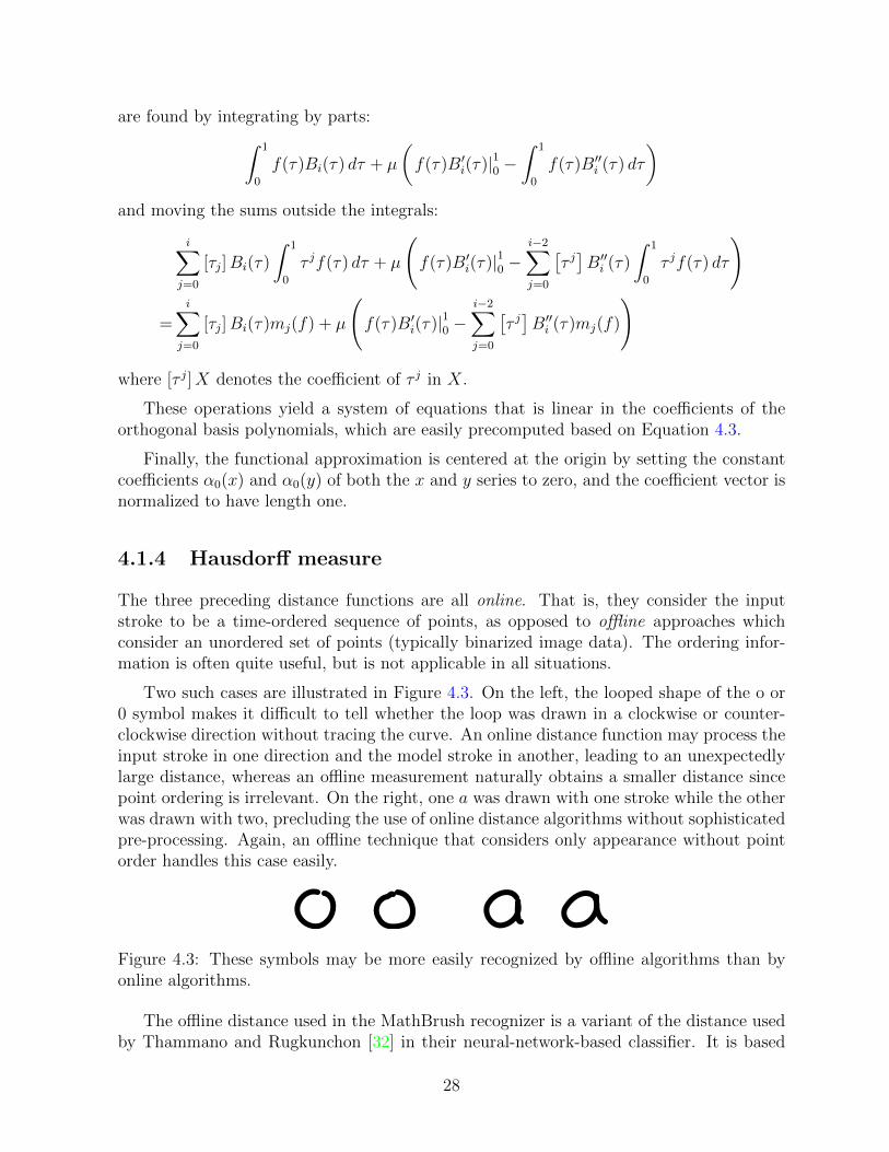
4.3 These symbols may be more easily recognized by offline algorithms than byonline algorithms. . . . . . . . . . . . . . . . . . . . . . . . . . . . . . . . . 28
4.4 Voting cannot choose between alternative groupings. . . . . . . . . . . . . 29
4.5 Distributions of the four distance measures. . . . . . . . . . . . . . . . . . 30
4.6 Symbol recognition accuracy. . . . . . . . . . . . . . . . . . . . . . . . . . . 32
5.1 The correct choice of relation depends on symbol identity. . . . . . . . . . 33
5.2 Hierarchical organization of semantic labels. . . . . . . . . . . . . . . . . . 34
5.3 θ function component of relation membership grade. . . . . . . . . . . . . . 36
5.4 Data clusters and splitting possibilities. . . . . . . . . . . . . . . . . . . . . 40
5.5 Relation classifier accuracy on 2009 data set. . . . . . . . . . . . . . . . . . 44
5.6 Relation classifier accuracy on 2011 data set. . . . . . . . . . . . . . . . . . 44
6.1 An expression in which the optimal relation depends on symbol identity. . 48
6.2 An expression demonstrating a variety of subexpression linkages. . . . . . . 52
7.1 An ambiguous mathematical expression. . . . . . . . . . . . . . . . . . . . 55
ix

7.2 Shared parse forest for Figure 7.1. . . . . . . . . . . . . . . . . . . . . . . . 56
7.3 Expressions with overlapping symbol bounding boxes. . . . . . . . . . . . . 59
7.4 Recursive rectangular partitions in an expression. . . . . . . . . . . . . . . 60
7.5 Illustration of expression extraction for a two-token production. . . . . . . 68
7.6 Interface for displaying and selecting alternative interpretations. . . . . . . 72
9.1 Default scenario results. . . . . . . . . . . . . . . . . . . . . . . . . . . . . 84
9.2 Perfect scenario results. . . . . . . . . . . . . . . . . . . . . . . . . . . . . . 84
x

List of Tables
3.1 Variables names for grouping concepts. . . . . . . . . . . . . . . . . . . . . 17
3.2 Grouping evaluation results. . . . . . . . . . . . . . . . . . . . . . . . . . . 21
5.1 Relational class labels. . . . . . . . . . . . . . . . . . . . . . . . . . . . . . 34
5.2 Angle thresholds for geometric relation membership functions. . . . . . . . 36
9.1 Evaluation on CROHME 2011 corpus. . . . . . . . . . . . . . . . . . . . . 86
9.2 Evaluation on CROHME 2012 corpus. . . . . . . . . . . . . . . . . . . . . 87
xi

Chapter 1
Introduction
Many software packages exist which operate on mathematical expressions. Such softwareis generally produced for one of two purposes: either to create two-dimensional renderingsof mathematical expressions for printing or on-screen display (e.g., LATEX, MathML), or toperform mathematical operations on the expressions (e.g., Maple, Mathematica, Sage, andvarious numeric and symbolic calculators). In both cases, the mathematical expressionsthemselves must be entered by the user in a linearized, textual format specific to eachsoftware package.
This method of inputting math expressions is unsatisfactory for two main reasons.First, it requires users to learn a different syntax for each software package they use.Second, the linearized text formats obscure the two-dimensional structure that is presentin the typical way users draw math expressions on paper. This is demonstrated with someabsurdity by software designed to render math expressions, for which one must linearize atwo-dimensional expression and input it as a text string, only to have the software re-createand display the expression’s original two-dimensional structure.
Mathematical software is typically used as a means to accomplish a particular goalthat the user has in mind, whether it is creating a web site with mathematical content,calculating a sum, or integrating a complex expression. The requirement to input math ex-pressions in a unique, unnatural format is therefore an obstacle that must be overcome, notsomething learned for its own sake. As such, it is desirable for users to input mathematicsby drawing expressions in two dimensions as they do with pen and paper.
Academic interest in the problem of recognizing hand-drawn math expressions orig-inated with Anderson’s doctoral research in the late 1960’s [2]. Interest has waxed andwaned in the intervening decades, and recent years have witnessed renewed attention to thetopic, potentially spurred on by the nascent Competition on Recognition of HandwrittenMathematical Expressions (CROHME) [25]. We will explore several recent contributionsto the field in the next chapter.
Math expressions have proved difficult to recognize effectively. Even the best state ofthe art systems (as measured by CROHME) are not sufficiently accurate for everyday useby non-specialists. The recognition problem is complex as it requires not only symbols
1

to be recognized, but also arrangements of symbols, and the semantic content that thosearrangements represent. Matters are further complicated by the large symbol set and theambiguous nature of both handwritten input and mathematical syntax.
My doctoral research has focused on this problem of recognizing handwritten mathe-matics in the context of the MathBrush project [13]. This thesis summarizes the theoryand implementation techniques developed to produce the recognition components of Math-Brush.
1.1 MathBrush recognizer overview
Before diving into technical details, it is worthwhile to explain the context of our mathrecognition system, as it grounds this research in a concrete, real-world application andplaces many useful and important constraints on the recognizer.
The math recognizer was developed for use in the MathBrush pen-math system, whichallows users to input mathematical expressions by drawing them on a Tablet PC or iPadtablet screen. Following the input step, the expression is embedded in a worksheet interfacein which the user may interact with it further by invoking computer algebra system (CAS)commands through context-sensitive menus, examining the results, and so on. As such, itis necessary for the recognizer to construct a semantic interpretation of the input so thatit may communicate effectively with the CAS; a syntactic representation of the input isinsufficient for this purpose.
The design goals of MathBrush emerged from earlier experiments [14] which discovered,unsurprisingly, that users became frustrated when incorrect recognition forced them toerase and re-write their input. This problem was exacerbated by a lack of feedback fromthe recognizer to indicate what had gone wrong, and by a disconnected recognition processin which symbols were recognized and then passed to a separate expression recognitionsystem, which could fail even if all the symbols were recognized correctly. As a result ofthese early experiments, the two primary goals of the current MathBrush system became:
1. To present the user with constant feedback about the state of the recognizer duringthe input process. In particular, the recognizer’s current “best guess” is updatedafter each new stroke is drawn.
2. To allow the user to easily correct any recognition errors without erasing and re-writing their input. This is accomplished by selecting alternative recognition resultsfrom drop-down menus.
The goals of MathBrush as a whole place three requirements on the recognizer. Thefirst is that, since recognition results are reported in real-time as the user writes, therecognizer should be fast enough to avoid an unreasonable delay between writing andviewing recognition results. This is the primary motivation for many of the simplifyingassumptions that will appear later in the thesis (see Chapter 7).
2

The second requirement is that users are able to train the recognizer to match theirhandwriting style. This is most important for symbol shapes (e.g., American vs. Europeanhandwriting styles). It must therefore be straightforward to adapt the recognizer to aparticular writing style. We comment on how such adaptation is possible in the MathBrushrecognizer in Section 4.1.
The final requirement is that users must be able to correct erroneous recognition results.This implies that, rather than recognizing ink input as a single, definite math expression,the recognizer should have the following capabilities:
1. to obtain and present multiple interpretations of a given input,
2. to correct a particular subexpression of an interpretation, and
3. to maintain that correction as writing continues.
These requirements significantly complicate the recognition problem, and motivate ourdevelopment of algorithms and data representations throughout the thesis, but particularlyin Chapters 6 and 7.
1.2 Two viewpoints on math recognition
Given a sequence of hand-drawn input strokes, each of which is itself an ordered sequenceof points in the plane, the math recognition problem is to represent the mathematicalexpression depicted by the strokes as a mathematical expression tree. From such a tree, thelinearized text formats described above may easily be obtained. Of course, one may allowfor more extensive input data – timings, pen pressure, tilt, and so on – but the structure ofthe problem remains the same, and most authors do not consider these additional sourcesof information because they are not reliably available on current hardware (touchscreendevices in particular).
Because of its complexity, it is worthwhile to break down the math recognition probleminto smaller subproblems which may be more easily analyzed. We adopt two distinctviewpoints for this purpose: an abstract, theoretical view, and a practical, system-builder’sview.
1.2.1 The abstract view
On a large scale, the math recognition problem can be divided in three: 1) to determinewhat mathematical content a group of the input strokes represents; 2) to decide whichof several interpretations of a group of strokes is the most plausible; and 3) to identifywhich groups of input strokes possess interpretations important to the structure of theexpression as a whole, and how those groups combine together. These three problems maybe conveniently called recognition, scoring, and searching. Together, they form a rubric
3

which serves to organize and focus discussion of the various inter-related parts of the mathrecognition problem.
These three subproblems are mutually dependent. To recognize a math expressionrequires an understanding of its constituent parts. To find those parts necessitates a searchthrough alternatives. To compare alternatives requires some means of scoring them. Tocombine parts into larger expressions requires an understanding of whether and how theparts fit together. Despite their dependence, though, each subproblem has a quite distinctstructure, and may be solved by distinct, independent strategies. Chapter 2 surveys severalexisting approaches to math recognition in terms of how researchers have addressed thesethree aspects of the problem.
1.2.2 The system-oriented view
Practical math recognition systems typically include a number of subsystems which arecombined through some unifying formalism. Symbol recognizers, relation classifiers, grammar-based parsers, and other components may each be a part of a larger math recognitionpackage. Each of these components may be implemented in many ways, and may have adifferent theoretical basis. For example, symbol recognition may be done via neural net-works, Markov models, similarity metrics, etc., whereas a stroke grouping system may usetiming information, convex hulls, and other geometric computations.
From the systems view, there are three high-level steps to solving the math recogni-tion problem: 1) identifying how to organize the math recognition system into smallersubsystems; 2) building and optimizing the accuracy and performance of each individualsubsystem; and 3) deciding how to combine the results of the subsystems into meaningfulmathematical output.
The first two of these points are fairly straightforward. The next section outlines thehigh-level system organization of the MathBrush recognizer, and the bulk of this thesis(Chapters 3 to 7) covers the implementation of recognition subsystems in detail. The thirdpoint on combining subsystems is more subtle. It is a significant practical challenge tocombine various subsystems in a way that both produces consistently meaningful results,and is theoretically sound. There is no a priori guarantee that the results produced byone subsystem are compatible with those produced by another, so effort is required whenintegrating recognition subsystems with one another. Chapter 8 examines our solution tothis issue of subsystem output compatibility through the MathBrush recognizer’s scoringframework.
1.3 Ambiguity and interpretation
Mathematical writing is inherently ambiguous at both the syntactic and semantic levels.Semantically, math is a relatively formal natural language [4] in which one statement oftenaffords multiple interpretations, depending on context. For example, the notation u(x+ y)could be either a function application or a multiplication (at least). Similarly, f ′ might
4

imply differentiation of a function, or it could simply be a variable related in some way toanother variable f .
These semantic ambiguities are impossible to resolve without contextual knowledge,and they are not addressed in this thesis. Rather, we assume a fixed set of supportedmathematical semantics, and report all recognized interpretations of the user’s writing sothat they may select the semantic interpretation they meant.
Syntactic ambiguity, though, is an unavoidable and interesting problem addressedthroughout this work. For example, the expressions shown in Figure 1.1 might be rea-sonably interpreted as Ax+ b, Axtb, Ax+ 6, and P x, pX.
Figure 1.1: Syntactic ambiguity in simple expressions.
In such cases, contextual knowledge is extremely helpful and is used by people whenreading mathematics. The answers to questions such as “which of P, p and t are knownto be variables?” and “is A a matrix and x a vector?” help to disambiguate the writing.Unfortunately, this contextual knowledge is not currently captured by MathBrush (or anyother math recognition software that we are aware of).
Informed by the interactive nature of MathBrush, we adopt a user-centric viewpointthat cuts across both the abstract and practical perspectives described above. When theuser writes an expression, they have a particular interpretation of their writing in mind.Rather than discarding the ambiguity present in the user’s writing and selecting a singleinterpretation of the input, we opt to capture that ambiguity as completely as is practical,and organize a variety of intepretations in such a way that it is easy for the user to selecttheir intended interpretation.
This decision influences the abstract subdivision of the math recognition problem intorecognition, searching, and scoring. Recognition maps syntax onto semantics, searching or-ganizes semantic interpretations into hierarchically-meaningful interpretation, and scoringorders those interpretations according to plausibility. Ideally, the highest-scoring interpre-tation of the input matches the user’s interpretation. But, because of imperfect recognitionalgorithms and the ambiguities just described, it is not possible for this to be the case allof the time.
In such cases, our goal is to make it as easy as possible for the user to obtain theirinterpretation from the recognizer. This is important in an interactive math system likeMathBrush because recognition itself is not the goal, but computation. The system mustunderstand the user’s interpretation for the subsequent mathematical operations to haveany meaning. The recognition process thus resembles a preliminary conversation ensuringthat the user and the system are on the same page, much as a student might ask a professorfor clarification on what an equation or variable represents before the professor goes througha proof during a lecture.
5

The requirement to capture and organize ambiguity in the input also poses significanttechnical challenges in terms of software construction. Much more data must be organizedthan if only a single interpretation was to be reported, which in turn makes it more difficultto attain real-time execution. The user-oriented viewpoint informs the design of recognitionalgorithms throughout our software, and much of the novel work in this thesis originatedfrom efforts to satisfy user-oriented requirements.
1.4 Contributions and thesis organization
In this thesis, we attempt to balance the abstract and system-oriented views describedearlier. My focus has been mainly on the system-building viewpoint, and the theory we havedeveloped plays largely a supporting role, explaining how to interpret the results of concretesystems, and how to combine those systems together. As such, this thesis documents theparticular recognition system we have constructed, developing and explaining what theoryis necessary as it progresses.
The recognizer consists of several primary subsystems:
• The stroke grouping system examines the input and identifies groups of strokes whichmay correspond to distinct symbols.
• The central parsing system searches for meaningful subdivisions and re-combinationsof the input according to a grammar which specifies valid mathematical syntax.
• The parsing system interacts with symbol and relation classification systems:
– The symbol classifier prepares a scored list of symbol identities that a particulargroup of input strokes is likely to represent.
– The relation classifier prepares a scored list of spatial relationships which a pairof input subsets are likely to satisfy (superscript, horizontally adjacent, etc.)
• The symbol classifier makes use of a symbol database which organizes and controlsaccess to a library of symbol examples written in various styles.
The rest of this thesis is organized as follows:
• The next chapter surveys related work in math recognition through the three-partrubric of recognition, searching, and scoring.
• Chapter 3 begins a sequence of three chapters on lower-level classification systemswith a look at the stroke grouping algorithms used in the math recognition system.This topic is rarely discussed in academic literature, but as the first and most low-level point of contact between MathBrush and the recognizer, its design has importantramifications throughout the recognition process.
6

• Chapter 4 covers symbol recognition, considering several individual classificationtechniques including a novel variant of the traditional elastic matching algorithm.This chapter also discusses the hybrid classification system developed for the Math-Brush recognizer.
• Chapter 5 discusses geometric relationship classification and completes our look atisolated classification problems. Several methods are explored and compared includ-ing rule-based and probabilistic approaches. A new data structure called the margintree is described and evaluated for the purpose of relation classification.
• Chapters 6 and 7 explore the theory and algorithms behind relational grammarsand two-dimensional parsing. We first develop a sophisticated extension of existingrelational grammar formalisms in Chapter 6, then describe in Chapter 7 some prac-tical constraints affording efficient parsing algorithms. We give both bottom-up andtop-down algorithms, describe how to simultaneously capture and represent multipleparse trees, and how to efficiently report those trees in decreasing score order.
• Chapter 8 develops fuzzy-set and probabilistic models of the recognition problemand applies them to the software systems described in earlier chapters. Each can beseen as a particular strategy for solving the abstract scoring problem, overlaid on thelower-level software systems. In the probabilistic case, an algebraic technique permitsefficient calculation of probabilities despite the large number of variables present inthe formal model.
• Chapter 9 wraps up the technical content of the thesis with two accuracy evaluationsof the recognition system. A novel user-based accuracy metric is employed, as wellas the detailed subsystem-oriented metrics from the Competition on Recognition OfHandwritten Mathematical Expressions (CROHME).
• Finally, Chapter 10 concludes the thesis with a summary of the research presentedand a look at promising areas for future research.
7

Chapter 2
Related work
Over the last four and a half decades, many researchers have examined the problem ofrecognizing hand-drawn math input. In this chapter, I will use the three-pronged rubric ofrecognition, searching, and scoring developed in Chapter 1 to review the math recognitiontechniques developed by several of these researchers, focusing on more recent work.
2.1 Anderson
Anderson developed a grammar model in which each rule was associated with one or morepredicates [2]. The predicates constrain the positions and sizes of the bounding boxes ofthe grammar rule’s right-hand side elements. For example, the grammar rule for a fractionmight include constraints specifying that the bottom of the bounding box of the numeratormust lie above the middle of the bounding box of the fraction bar, which must in turn lieabove the top of the bounding box of the denominator.
Anderson assumes that the symbols comprising the math expression have already beenrecognized with no errors or ambiguity. His input consists of bounding boxes labeledwith symbol names. To obtain the math expression represented by a particular symbolarrangement, a depth-first search (DFS) is performed. Starting with the first grammar rule,each symbol is assigned to a RHS element such that the rule’s constraints are satisfied, andthen the algorithm recurses on each RHS element. If no assignment exists which satisfiesany relevant rule’s constraints, the algorithm backtracks. When a complete expressiontree is detected, it is reported and the algorithm terminates. The grammar rules musttherefore be carefully ordered so that the “correct” expression is selected before an incorrectexpression is detected. (E.g., the rule for sin must appear before the multiplication rule toprevent sin being recognized as a multiplication.)
Anderson thus solves the recognition problem by assigning meaning to symbols throughthe semantic interpretation of his grammar rules, and he solves the searching problem quiteliterally through a depth-first search of the possible subdivisions of the input into smallersemantic units. His system does not compare alternative interpretations of the input,but merely reports the first valid interpretation it discovers, so he does not address the
8

scoring problem. While the system is impressive for its generality (Anderson also givesgrammars for recognizing matrices and labeled graphs), it is ultimately inefficient (becauseof the DFS) and brittle (because of hard-coded grammar predicates and the dependenceon grammar order).
2.2 Zanibbi
Some decades after Anderson’s seminal work, Zanibbi proposed a three-pass math recog-nizer based on the notion of baseline structure trees (BST) [38]. The first pass – the layoutpass – is the most important. In it, baselines in the input are identified and structured in atree that represents their hierarchical relationship with one another. For example, the frac-tion expression a
bwould be represented by a tree with the fraction bar as the root node, and
two children, labeled “above” and “below” representing the numerator and denominator.
These baseline trees are obtained by determining which symbols represent mathematicaloperators which “dominate” other symbols. (E.g., the fraction bar dominates the a andb symbols, as they are arguments to its operation.) Dominated symbols are assigned tospatial regions afforded by the dominating operators by means of thresholds on boundingbox position. (E.g., the fraction bar affords “above” and “below” regions, and symbolsdominated by the fraction bar are assigned to one of those regions by comparing thesymbols’ vertical centroids with the fraction bar’s bounding box.) This process of assigningsymbols to baseline tree nodes is somewhat less flexible than Anderson’s predicate-basedapproach, but it is also much faster. BST construction is Zanibbi’s solution to the searchingproblem.
The lexical pass transforms the BST created by the layout pass by grouping togetherover-segmented symbols (e.g., two horizontal lines might be combined into =) and group-ing related symbols (e.g., the individual numbers 2 and 2 might be combined to form 22).Finally, the expression pass applies tree transformations to convert the BST into a mathexpression tree. One could say that Zanibbi solves the recognition problem by associatingparticular BST tree patterns with math semantics. However, in this case, the recognitionprocess appears to an extent in all three passes. The first pass is largely devoid of recogni-tion, being concerned solely with syntactic features, yet the rules used to generate baselinetrees assume that mathematical semantics will be applied. So recognition is taking placeto some extent when, for example, the algorithm searches for symbols above and below afraction bar. The second pass also performs recognition, as it groups related syntactic unitstogether into larger semantic groups such as function names and floating-point numbers.
Like Anderson, Zanibbi assumes that the input strokes have already been grouped intodistinct symbols and recognized with no errors. Ambiguity in his system is only possiblewhen the spatial regions of two or more operators overlap. In such cases, hard-coded rulesare used to assign symbols in ambiguous regions to one region or another. Scoring is thusobviated in Zanibbi’s work as any ambiguity is eliminated a priori.
9

2.3 Winkler, Farhner, and Lang
Winkler, Farhner, and Lang also assume that symbols have already been recognized per-fectly [35]. They solve the searching problem similarly to Zanibbi, by identifying symbolsthat represent math operators and assigning dominated symbols to spatial regions aroundthe math operator. (In fact, the work of Winkler et al. predates that of Zanibbi.) Unlikeboth works discussed above, though, Winkler et al. address the scoring problem and hencepermit their system to choose between multiple interpretations of the same input.
They do this by taking the reciprocals of the distances that a dominated symbol wouldneed to be shifted in order for its bounding box to lie completely within each of thedominating symbol’s pre-defined spatial regions. These reciprocals are then normalizedand treated as probabilities. Using our example a
b, the fraction bar possesses three regions:
“above” and “below” as in Zanibbi’s work, and also “out”, which links to the next symbolin the same baseline.
In the case of fractions, only the most probable result is used. This is, in effect,identical to not using scoring at all. Although multiple candidates are considered, onlyone is used, and it is determined a priori by the distance calculations used to generate theprobabilities. More interestingly, Winkler et al. permit symbols to participate ambiguouslyin superscripts, subscripts, and in-line relations. Each possibility is assigned a probablity,as with the above and below relations just discussed. But rather than discarding everythingbut the most probable option, each possible relation leads to a different parse, and all parsesare reported to the user. Winkler et al. apply thresholds to the probabilities in order tolimit the number of parses reported, which is naively exponential in the number of inputsymbols.
The searching procedure of Winkler et al. thus has the same basis as that of Zanibbi,but is made more sophisticated through its allowance for ambiguous relations. It can beviewed as searching through the space of directed acyclic graphs (DAGs) with the symbolsas nodes, and edges labeled with the relations linking the symbols.
Like Zanibbi, Winkler et al. only assign semantic meaning to symbols and relationsas a final step, when the DAG generated by their algorithm may be converted into anexpression tree. But, as we saw with Zanibbi’s work, recognition is implied in the earlierstages of the algorithm, which organize the symbols and relations based on the assumptionthat they possess mathematical significance.
2.4 Miller and Viola
Miller and Viola expanded upon the ambiguity permitted by Winkler et al. [24]. In theirsystem, symbol recognition was not assumed to be complete and perfect. In fact, as wellas permitting ambiguous relations between symbols, Miller and Viola permit the symbolsthemselves to be ambiguous. They introduced the notion of a syntactic class which capturesthe expected position of a symbol with respect to its baseline. For example, the number 9extends from the baseline to the “top line”, the letter c from the baseline to the “mid line”,
10

and the letter q from below the baseline to the mid line. Miller and Viola use syntacticclasses to manage ambiguity in symbol identity by seeding their parsing algorithm withthe top-ranked alternative from each class for each symbol. They do not describe how thesymbol recognition itself is performed, nor how the input strokes are grouped into distinctsymbols.
The parsing algorithm itself proceeds in a bottom-up fashion. Beginning with theseeded symbols, it combines recognized subsets of the input to form larger recognized setsby applying grammar rules, similarly to the CYK algorithm for parsing CFGs. Ratherthan exhausting all possible subsets combinations, Miller and Viola introduce two keyideas to limit the search space. The first is a hard constraint that requires any set ofstokes considered by the algorithm to have no other stroke intersecting its convex hull.This constraint was later expanded upon by Liang et al. who used rectangular hulls andpartial-ordered sets for a similar purpose [18].
The second idea of Miller and Viola is to use the A-star search algorithm to guide theparser’s choice of subset combinations. They use the negative log likelihood as the under-estimate of the “distance” to the search goal. Assuming independence of all symbols andrelations, they treat the symbol recognition results probabilistically, and model relationsbetween symbols as two-dimensional Gaussians. This approach builds on earlier work ofHull [12].
The parsing algorithm therefore performs a best-first search as it combines subsetswhich satisfy the convex hull criterion. In this way, scoring is integrated into the searchprocess as a guiding factor, and recognition is a by-product of applying grammar rulesduring subset combination. Compared with previous work, the search process has againbecome more sophisticated, and the scoring more comprehensive and systematic.
2.5 Garain and Chaudhuri
In 2004, Garain and Chaudhuri proposed another system incorporating both symbol andexpression recognition [7]. In it, symbols are recognized by measuring the distance andangle between consecutive points in each input stroke. These features are compared againsttemplate strokes by two classifiers (a feature vector classifier, and a hidden Markov model(HMM) classifier), the results of which are combined to obtain final recognition results.Symbols are recognized immediately as they are drawn, but Garain and Chaudhuri do notdescribe how the system determines that a symbol is complete. For example, after threestrokes, an E may look exactly like an F, and it is not clear whether the system is able torevise its previous recognition results to account for this.
In any case, after a symbol is drawn and recognized, it is assigned to a particular “level”of the expression. The expression’s main baseline, to which the first symbol is assumedto belong, is level 0, and higher or lower levels represent writing lines above and belowthe main baseline. Levels are not directly analogous to baselines. For example, in theexpression 2nex, the symbols n and x are distinct baselines, but are both on level 1 usingGarain and Chaudhuri’s terminology.
11

By ordering symbols horizontally, spatial relations such as superscripts, subscripts, andhorizontal alignment are determined by the level assignments. Mathematical semanticsare directly associated with these relationships. More complex relationships like limits ofintegration are found by segmenting the input strokes into vertical and horizontal “stripes”,or contiguous regions, and then using a grammar to guide stripe recombination. Somespecialized rules are invoked for vertical structures such as summations with limits. ThusGarain and Chaudhuri use a combination of baseline analysis and rectangular regions tosolve the searching problem.
The system uses scoring to an extent when ranking symbol recognition results. But itdoes not discriminate between alternatives so much as reject invalid choices. After recog-nizing the input using the top-ranked symbol recognition results, the LATEX representationof the recognized expression is compared against a validation grammar. If validation fails,alternative character recognition results are explored, though it is not entirely clear howthis search through alternatives proceeds.
2.6 Laviola, Zeleznik et al.
The MathPad project at Brown University ([17, 40]) was a long-running research pro-gramme for creating math sketching systems. Its high-level goals differ from those ofMathBrush in that the Brown project aims to facilitate learning and problem-solvingthrough interactive sketches controlled by mathematical formulae, while MathBrush in-tends to be a research tool for mathematicians and students. However, many softwarefeatures required to attain each of these goals are similar, and so MathPad includes amath recognition system.
MathPad’s recognition system may be viewed as an informal application of grammar-based parsing. Rules governing how symbols are arranged into math expressions are ex-plicitly coded into the program. Input is processed in a way analagous to how a particularorganization of grammar productions could be naively parsed. The recognition system in-cludes sophisticated heuristics specialized to particular mathematical structures (fractions,integrals, etc.). While this approach is highly tunable, it is less flexible than other, lessexplicitly-specified approaches.
A study of the recognition accuracy of MathPad was presented by LaViola [16]. In thestudy, 11 subjects individually provided the system’s symbol recognizer with 20 samplesof their handwriting for each supported symbol. Each subject then provided 12 additionalsamples of each symbol as well as drawings of 36 particular math expressions as testdata. The expressions were partly taken from Chan and Yeung’s collection [6] and partlydesigned by the author. This data was used to test MathPad’s symbol recognizer and mathexpression parser, respectively. Laviola measured the proportion of symbols recognizedcorrectly and the proportion of parsing decisions which were correct. A parsing decisionarises in LaViola’s system whenever symbols must be grouped together (or not) into asubexpression (e.g., tan as multiplication versus the function name tan) or a choice mustbe made about the type of a subexpression (e.g., superscript vs. inline)
12

2.7 Alvaro et al.
The system developed by Alvaro et al. [1] placed first in the CROHME 2011 recognitioncontest [25]. It is based on earlier work of Yamamoto et al. [36]. A grammar modelsthe formal structure of math expressions. Symbols and the relations between them aremodeled stochastically using manually-defined probability functions. The symbol recogni-tion probabilities are used to seed a parsing table on which a CYK-style parsing algorithmproceeds to obtain an expression tree representing the entire input.
In this scheme, writing is considered to be a generative stochastic process governed bythe grammar rules and probability distributions. That is, one stochastically generates abounding box for the entire expression, chooses a grammar rule to apply, and stochasticallygenerates bounding boxes for each of the rule’s RHS elements according to the relationdistribution. This process continues recursively until a grammar rule producing a terminalsymbol is selected, at which point a stroke (or, more properly, a collection of stroke features)is stochastically generated.
Given a particular set of input strokes, Alvaro et al. find the sequence of stochas-tic choices most likely to have generated the input. However, stochastic grammars areknown to biased toward short parse trees (those containing few derivation steps) [23]. Inour own experiments with such approaches, we encountered difficulties in particular withrecognizing multi-stroke symbols in the context of full expressions. The model has no in-trinsic notion of symbol segmentation, and the bias toward short parse trees caused therecognizer to consistently report symbols with many strokes even when they had poorrecognition scores. Yet to introduce symbol segmentation scores in a straightforward waycauses probability distributions to no longer sum to one. Alvaro et al. allude to similar dif-ficulties when they mention that their symbol recognition probabilities had to be rescaledto account for multi-stroke symbols.
2.8 Awal et al.
While the system described by Awal et al. [3] was included in the CROHME 2011 contest,its developers were directly associated with the contest and were thus not official partici-pants. However, their system scored higher than the winning system of Alvaro et al., so itis worthwhile to examine its construction.
A dynamic programming algorithm first proposes likely groupings of strokes into sym-bols, although it is not clear what cost function the dynamic program is minimizing. Eachof the symbol groups is recognized using neural networks whose outputs are converted intoa probability distribution over symbol classes.
Math expression structure is modeled by a context-free grammar in which each rule islinear in either the horizontal of vertical direction, simplifying the search problem. Spa-tial relationships between symbols and subexpressions are modeled as two independentGaussians on position and size difference between subexpression bounding boxes. These
13

probabilities along with those from symbol recognition are treated as independent variables,and the parse tree with maximal likelihood is reported as the final parse.
This method as a whole is not probabilistic as the variables are not combined in acoherent model. Instead, probability distributions are used as components of a scoringfunction. This pattern is common in the math recognition literature: distribution functionsare used when they are useful, but the overall strategy remains ad hoc.
2.9 Shi, Li, and Soong
Working with Microsoft Research Asia, Shi, Li, and Soong proposed a unified HMM-basedmethod for recognizing math expressions [29]. Treating the input strokes as a temporally-ordered sequence, they use dynamic programming to determine the most likely points atwhich to split the sequence into distinct symbol groups, the most likely symbols each ofthose groups represent, and the most likely spatial relation between temporally-adjacentsymbols. Some local context is taken into account by treating symbol and relation se-quences as Markov chains. This process results in a DAG similar to one obtained byWinkler et al., which may be easily converted to an expression tree.
To compute symbol likelihoods, a grid-based method measuring point density and strokedirection is used to obtain a feature vector. These vectors are assumed to be generated bya mixture of Gaussians with one component for each known symbol type. Relation like-lihoods are also treated as Gaussian mixtures of extracted bounding-box features. Grouplikelihoods are computed by manually-defined probability functions.
This approach is elegant in its unity of symbol, relation, and expression recognition.The reduction of the input to a linear sequence of strokes drastically simplifies the searchproblem, while probabilistic rules and the probabilistic models selected by the authorsconstitute a scoring mechanism. The interpretations associated with particular assignmentsof the model’s variables provide recognition, in combination with the features selected forextraction.
But this assumption of linearity comes at the expense of generality. The HMM structurestrictly requires strokes to be drawn in a pre-determined linear sequence. That is, the modelaccounts for ambiguity in symbol and relation identities, but not for the two-dimensionalstructure of mathematics.
14

Chapter 3
Stroke grouping
The role of the stroke grouping system is to determine, given a set of ink strokes, whichsubsets of those strokes correspond to distinct symbols. For example, numbering the strokesin Figure 3.1 1,2,3,4,5 from left to right, the stroke grouper should report {1} , {2, 3} , {4, 5}as likely symbols. This task, though necessary for any handwriting recognition system, isgenerally neglected in most publications. Note that the identities of those symbols (i.e., a,+, and b) is irrelevant here. We are concerned only with proposing reasonable subsets ofthe ink as candidates for symbol recognition.
Figure 3.1: A simple input for the stroke grouper.
Figure 3.1 might suggest that this task is straightforward, so consider the input shownin Figure 3.2. It is difficult to determine whether this input is supposed to represent aoHor ad − 1, even for a mathematically-literate human. But the user who drew this inputpresumably knew what they intended it to represent. We will rely in such cases on ourstrategy of presenting the user with several reasonable interpretations of their input so thatthey can select the one they intended.
Figure 3.2: A more difficult input for the stroke grouper.
It is vitally important for the grouper to avoid false negatives. If an ink subset thatcorresponds to a symbol in the user’s interpretation of the ink is not reported by the strokegrouping system, then that subset will not be subject to symbol recognition, and will not beincluded in any recognition results. Therefore, false negatives preclude correct recognitionof the input and should be avoided at all costs.
15
The example in Figure 3.2 indicates that the grouper need not limit itself to a singlepartitioning of the ink into symbol groups. Rather, any subset of the input that couldreasonably be considered a distinct symbol should be reported, so as to maximize thelikelihood of identifying the user’s preferred interpretation of their writing.
These two observations imply that false positives are acceptable. That is, it is accept-able for the grouper to identify as a potential symbol a subset of the input which does notactually correspond to a symbol in the user’s interpretation. We may reasonably assumethat many false positives will be filtered out by later stages of recognition. As an extremeexample, suppose the stroke grouping system identifies the a+ portion of Figure 3.1 as apotential symbol. These strokes are unlikely to be recognized with high confidence as asingle symbol. So long as the grouper also proposes the a and + subsets individually aspotential symbols, overall recognition should still give the result the user expects.
To summarize, the role of the stroke grouper is to select subsets of the input for symbolrecognition such that all subsets corresponding to symbols in the user’s interpretation ofthe input are included. The rest of this chapter describes and evaluates our techniques foraccomplishing this goal.
3.1 Relevant input characteristics
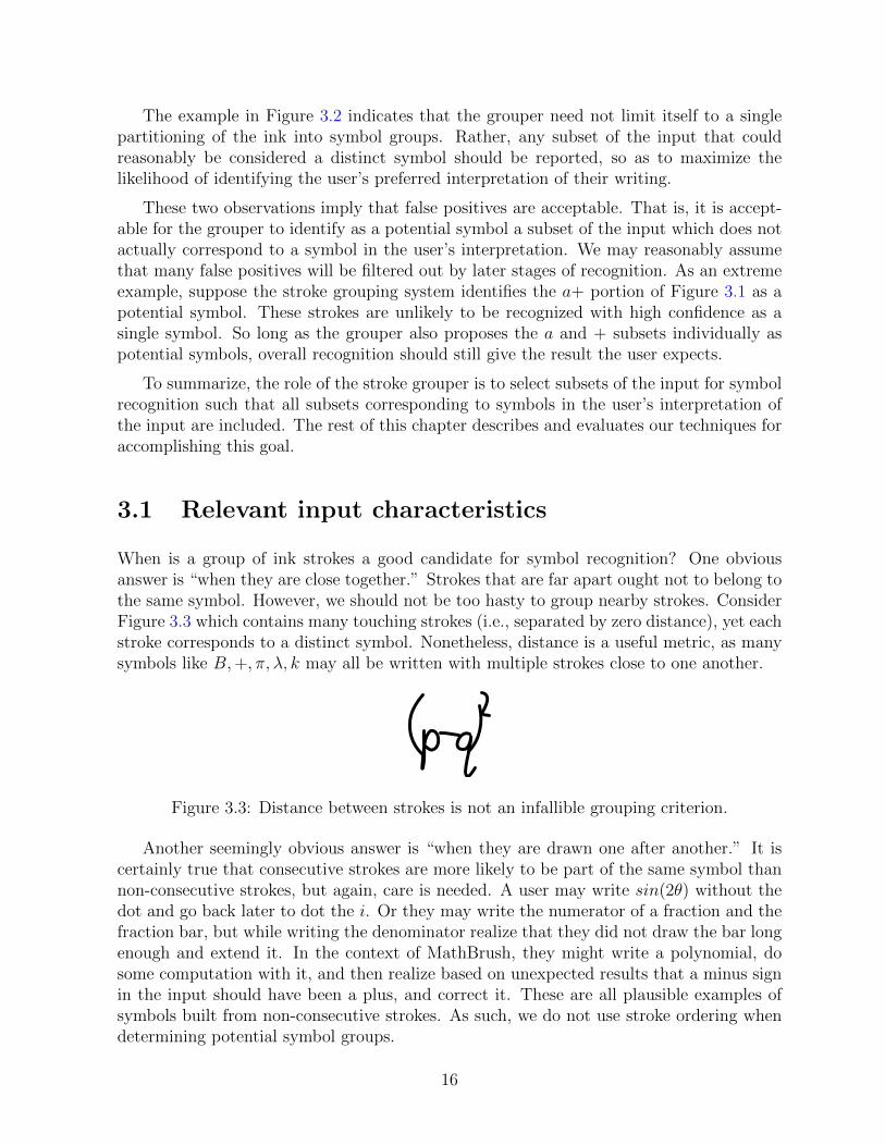
When is a group of ink strokes a good candidate for symbol recognition? One obviousanswer is “when they are close together.” Strokes that are far apart ought not to belong tothe same symbol. However, we should not be too hasty to group nearby strokes. ConsiderFigure 3.3 which contains many touching strokes (i.e., separated by zero distance), yet eachstroke corresponds to a distinct symbol. Nonetheless, distance is a useful metric, as manysymbols like B,+, π, λ, k may all be written with multiple strokes close to one another.
Figure 3.3: Distance between strokes is not an infallible grouping criterion.
Another seemingly obvious answer is “when they are drawn one after another.” It iscertainly true that consecutive strokes are more likely to be part of the same symbol thannon-consecutive strokes, but again, care is needed. A user may write sin(2θ) without thedot and go back later to dot the i. Or they may write the numerator of a fraction and thefraction bar, but while writing the denominator realize that they did not draw the bar longenough and extend it. In the context of MathBrush, they might write a polynomial, dosome computation with it, and then realize based on unexpected results that a minus signin the input should have been a plus, and correct it. These are all plausible examples ofsymbols built from non-consecutive strokes. As such, we do not use stroke ordering whendetermining potential symbol groups.
16

Note that all of the cases just described follow a pattern in which some strokes fora symbol are drawn, then some unrelated strokes are drawn, then some strokes for thatsymbol are added and are nearby the original strokes. So stroke proximity alone is able tocapture these patterns.
In some cases, such as in the π and F symbols shown in Figure 3.4, not all of the strokesmaking up a symbol will be near to one another. Or at least, the distance between thestrokes will be large enough that it is quite ambiguous whether the strokes belong to thesame symbol, or whether the writing is just closely spaced, as in Figure 3.3. In these cases,though, it is often the case that the bounding box of each stroke has a large intersectionwith the bounding box of the other strokes.
Figure 3.4: Bounding box overlap is another good indicator of stroke groups.
Bounding box overlap is thus another useful feature to consider when grouping strokes.But here too care is needed. Some symbol arrangements, in particular the syntax forsquare roots, cause large bounding box intersections but ought not to be grouped together,as shown in Figure 3.5. So large bounding box intersections should suggest symbol groupingunless a square root or other containment notation is involved. Conversely, a group shouldnot have a large overlap with strokes outside of the group, unless a containment notationis involved.
Figure 3.5: Bounding box overlap is not always a reason to group strokes into symbols.
Labeling the concepts in this discussion as shown in Table 3.1, the following logicalequation summarizes the characteristics of a “good” group identified above:
G = (Din ∨ (Lin ∧ ¬Cin)) ∧ (¬Lout ∨ Cout) (3.1)
Name MeaningG A group existsDin Small distance between strokes within groupLin Significant bounding box overlap of strokes within groupCin Containment notation used within groupLout Significant bounding box overlap of group and non-group strokesCout Containment notation used in group or overlapping non-group strokes
Table 3.1: Variables names for grouping concepts.
Because of the ambiguity of handwritten input and the requirement of avoiding falsenegatives, it is unreasonable to assign binary values to the variables in 3.1. Instead, we
17

assign quantitative scores to the variables in a probabilistic evaluation scheme. This processis described below.
3.2 Grouping algorithm
Because the MathBrush recognizer receives input strokes one-by-one from the interface,we formulate the grouping problem as follows. Given a set of existing stroke groupingcandidates (not necessarily a partition of the input; i.e., the groups may overlap) and anew input stroke, find a new set of grouping candidates incorporating the new stroke. Thisamounts to identifying the existing groups to which the new stroke may be reasonablyadded, and potentially augmenting those new groups with existing strokes. This secondaugmentation step is necessary because of cases like the π shown in Figure 3.4. If thetwo vertical strokes of π are first drawn fairly far apart, it is unlikely that they will beidentified as being part of the same symbol. Only after the third stroke is drawn can theentire symbol be reliably identified.
At a high level, group identification proceeds according to Algorithm 1.
Algorithm 1 High-level stroke grouping algorithm.
Require: A set S = {s1, . . . , sn} of input strokes and a set G = {g1, . . . , gN} of subsets ofS \ {sn}Initialize G′ ← {}(add sn to existing groups)for each group g ∈ G do
if score(g, sn) > 0 thenadd g ∪ {sn} to G′
(augment new groups with existing strokes)while G′ 6= {} doG← G ∪G′;G′′ ← {}for each group g ∈ G′ and each stroke s ∈ S such that s 6∈ g do
if score(g, s) > 0 thenadd g ∪ {s} to G′′
G′ ← G′′
The interesting portion is, of course, the score function referenced by the algorithm.The value of score(g, s) corresponds to augmenting a group g with a stroke s. To computeit, we take several measurements of the inputs:
• d = min {dist(s′, s) : s′ ∈ g}, where dist(s1, s2) is the minimal distance between thecurves traced by s1 and s2;
• `in = overlap(g, s), where overlap(g, s) is the area of the intersection of the boundingboxes of g and s divided by the area of the smaller of the two boxes;
18

• cin = max (C(s),max {C (s′) : s′ ∈ g}), where C (s) returns the extent to which thestroke s resembles a containment notation, as described below;
• `out = max {overlap(g ∪ {s}, s′) : s′ ∈ S \ (g ∪ {s})};
• cout = max (cin, C (s′)), where s′ is the maximizer for `out.
To account for containment notations in the calculation of cin and cout, we annotateeach symbol supported by the symbol recognizer with a flag indicating whether it is usedto contain other symbols. (Currently only the
√symbol has this flag set.) Then the
symbol recognizer is invoked to measure how closely a stroke or group of strokes resemblesa container symbol. The details of how this is done will be discussed in the next chapterwhich covers symbol recognition. For now, we simply model the symbol recognizer as afunction C(T ) of a set T of strokes that returns a value in [0, 1] indicating the degree towhich T resembles a container, with 0 being not at all and 1 being a very close resemblance.
Using DeMorgan’s law, the logical predicate in Equation 3.1 can be rewritten as
G = ¬ (¬Din ∧ ¬ (Lin ∧ ¬Cin)) ∧ ¬ (Lout ∧ ¬Cout)= ¬ (¬Din ∧ ¬Xin) ∧ ¬Xout,
where X∗ = L∗ ∧ ¬C∗.This predicate may be transformed into a probability calculation by defining conditional
distributions. We set
score(g, s) = P (G | d, `in, cin, `out, cout)= (1− P (¬Din | d)P (¬Xin | `in, cin))β P (¬Xout | `out, cin, cout)1−β (3.2)
where
P (¬Din | d) =(1− e−d/λ
)αP (¬Xin | `in, cin) = (1− `in (1− cin))(1−α)
P (¬Xout | `out, cout, cin) = 1− `out (1−max (cin, cout)) .
This definition is loosely based on treating the boolean variables from our logical pred-icate as random and independent. λ is estimated from training data, with α, β both setbased on experiments to 9/10.
Notice that each of the measurement variables is only defined for multiple strokes. Itremains to handle single-stroke groups so that one-stroke symbols will be recognized. Todo so, denote the score of a multi-stroke group g by
score (g) = max {score (g′, si) : g′ ∪ {si} = g} .
Often this score will coincide with the value score (g′, sn) computed in the first half ofAlgorithm 1 (where g = g′ ∪ {sn}). But because of the augmentation step in the second
19
half of the algorithm, it is possible for the same group to be obtained through differentsequences of stroke addition, so the maximization is necessary.
Now for each individual stroke s, we simply create a default group gs with score
score(gs) = 1−max {score(g) : g ∩ gs 6= {}} .
As each input stroke is received by the MathBrush recognizer, Algorithm 1 is used toaugment the existing set of candidate symbols by incorporating the new stroke. All of theresulting groups, along with their scores, are forwarded to the symbol recognition systemfor subsequent processing and scoring.
3.3 Evaluation
The grouping algorithm is somewhat difficult to evaluate in isolation because it is designedto be used in conjunction with higher-level recognition systems like symbol recognizers. Ihave employed two correctness metrics:
1. Basic: a symbol is grouped correctly if its group score is non-zero.
2. Strict: a symbol is grouped correctly if its group score is higher than all other groupssharing strokes with the symbol.
These metrics respectively represent upper and lower bounds on the real-world per-formance one can expect from the grouping algorithm. The basic metric overestimatesthe algorithm’s performance because some groups with non-zero scores will be scored toolow for higher-level recognizers to recover from; those groups will not be reported as sym-bols during regular use. But the strict metric underestimates the algorithm’s performancebecause of our expectation of false positives: if the correct group has a score close toan intersecting but incorrect group’s score, the symbol recognizer will very often preferthe lower-scoring group because the incorrect group has no reasonable symbol recognitionresults.
The grouping algorithm and score functions defined above were evaluated on a dataset collected in 2009 [20] consisting primarily of randomly-generated math expressionstranscribed by twenty undergraduate students. The data was randomly divided roughlyin half, with one half used for training and the other for testing. The stroke groupscorresponding to symbols in the training data were extracted and used to obtain thescoring function parameter λ, then the grouping algorithm was applied to the test files andthe two metrics above were measured. This experiment was replicated five times with fivedifferent splits of the data. The evaluation results are shown in Table 3.2.
These results indicate that the grouping algorithm reports over 99% of symbols, andscores roughly 90% of actual groups higher than all false positives. We will see in Chapter9 that, in the context of full math expression recognition, the grouping algorithm’s outputresults in about 97% of symbols being grouped correctly.
20
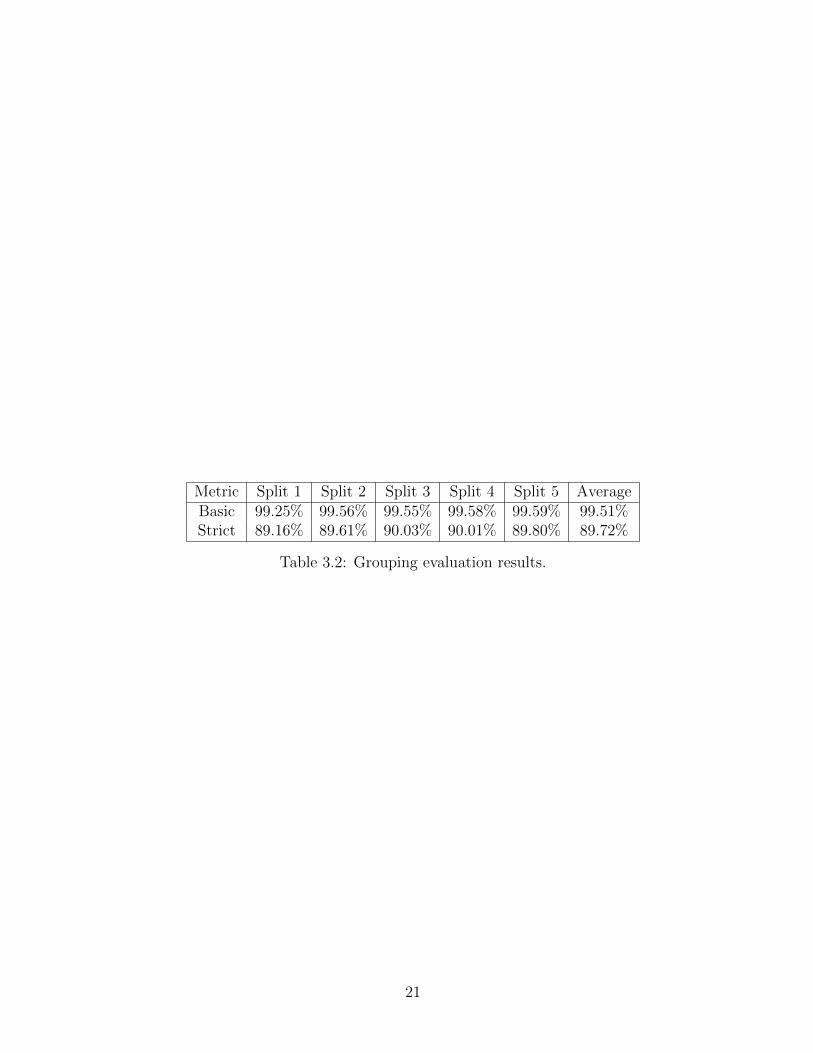
Metric Split 1 Split 2 Split 3 Split 4 Split 5 AverageBasic 99.25% 99.56% 99.55% 99.58% 99.59% 99.51%Strict 89.16% 89.61% 90.03% 90.01% 89.80% 89.72%
Table 3.2: Grouping evaluation results.
21

Chapter 4
Symbol recognition
The role of the symbol recognition system is to examine the input subsets identified bythe grouping system as potential symbols, and to determine which symbols, if any, thosegroups represent. These results are, in turn, incorporated into higher-level systems whichidentify mathematical expressions in the input.
4.1 Recognition algorithms
All of the symbol recognition algorithms discussed in this chapter follow the same distance-based classification paradigm. In this scheme, one uses a distance function d(I,M) to mea-sure the difference between a set I of input strokes and each set M of model strokes takenfrom a library L of labeled symbol models. Then I is recognized by d as the label attachedto argmin {d (I, g) : g ∈ L}. This approach is easily extended to report ordered lists of thek best recognition candidates. It also easily handles writer-dependent training, as symbolsdrawn by a particular user may simply be added to the library to adapt recognition to theuser’s writing style.
For the first three (online) algorithms below, we define the set-wise distance functionabove in terms of an algorithm-specific stroke-wise distance function:
d(I,M) =
{∞ if |I| 6= |M |∑
s∈I d(s,fI,M (s))|I| otherwise
(4.1)
where fI,M is a function mapping each input stroke in I to the corresponding model strokein M . This mapping is necessary to handle situations in which the strokes comprisingthe input symbol are drawn in a different order than those comprising the model symbol.Its construction will be discussed in Section 4.1.1. For the final (offline) algorithm, thenumber of input strokes need not match the number of model strokes, so the case yieldingan infinite distance is unnecessary.
In cases where the stroke-wise distance function is not symmetric (d(s1, s2) 6= d(s2, s1)),we average the results of both match directions so that the second case of Equation 4.1
22

becomes1
2
(∑s∈I d (s, fI,M (s))
|I|+
∑s∈M d (s, fM,I (s))
|M |
)(4.2)
Prior to invoking the distance function, both I and M are normalized such that thelargest side of their bounding box has length 1. Next we will describe each of the fourdistance functions used by the recognizer.
4.1.1 Feature vector norm
The first distance function is the simplest. We define several functions f1(s), f2(s), . . . , fn(s),each measuring some feature of a stroke as a real number, and take
d (a, b) =
√√√√ n∑i=1
(fi(a)− fi(b))2,
that is, the 2-norm of the vector of feature differences. We employ two sets of features:one for use with small punctuation marks, and the other for the general case.
• Small symbol features: aspect ratio; distance between stroke endpoints.
• Standard features: bounding box position and size; first and last point; lengthalong stroke.
The function fI,M matching up strokes between the input and model stroke sets isdefined greedily using this feature vector distance function, as follows:
1. Pick a stroke a ∈ I.
2. Find the stroke b ∈ M minimizing d(a, b), where d is the feature vector distancefunction. Set fI,M(a) = b and remove a and b from consideration in future processing.
3. Repeat until no unmatched input strokes remain.
4.1.2 Greedy elastic matching
The use of elastic matching goes back to Tappert [31], who developed it as a technique forrecognizing cursive writing. In the standard formulation, each point in the input strokeis matched with a point in the model stroke and a pointwise distance measure is appliedto each matched pair. The stroke-wise distance function is then the sum of pointwisedistances between matched pairs. Tappert’s algorithm finds the minimal such distance,subject to the three following constraints:
1. The first input point is matched to the first model point;
23

2. The last input point is matched to the last model point; and
3. If the ith input point is matched to the jth model point, then the i+ 1st input pointis matched to the jth, j + 1st, or j + 2nd model point.
Let the input stroke be the sequence of points {(xi, yi) : i = 1, . . . , n} and the modelstroke be the sequence {(xi, yi) : i = 1, . . . ,m}. Given a distance function g(i, j) betweenthe points (xi, yi) and (xj, yj), the above constraints induce the dynamic program D[i, j],representing the minimal distance between model points 1 through i and input points 1through j, as follows:
D[1, j] = g(1, j) +D[1, j − 1]
D[2, j] = g(2, j) + min {D[2, j − 1], D[1, j − 1]}D[i, j] = g(i, j) + min {D[i− k, j − 1] : k = 0, 1, 2}
Note that many distance functions g are possible. For cursive writing, Tappert uses
g(i, j) = min{∣∣∣θi − θj∣∣∣ , ∣∣∣360−
(θi − θj
)∣∣∣}+ α |yi − yj| ,
where θi is the tangent angle at (xi, yi) and α is chosen so that the angular and y-coordinatecomponents of the sum have equal weight.
Tappert gave a quadratic-time dynamic programming algorithm to find the elasticmatching distance between two strokes. Each dynamic programming table cell requiresonly constant time to compute, but there are O(nm) ≈ O(n2) table cells to be computedand stored. In the context of math recognition, the symbol library is quite large because ofthe presence of Greek letters and mathematical symbols, and symbol recognition processesmay be invoked several times if there are several ways to partition a large input into distinctsymbols. We found that the quadratic matching time per stroke consumed a significantproportion of total processing time in MathBrush, prompting our development of a fastervariant.
Greedy elastic matching
We motivate our algorithm by some straightforward observations about Tappert’s con-straints. Let I1, I2, . . . , In be the points comprising the input stroke, and M1,M2, . . . ,Mm
be similar for the model stroke. According to constraints 1 and 2, I1 must be matchedto M1 and In must be matched to Mm. By constraint 3, I2 must be matched to one ofM1,M2,M3, and In−1 must be matched to one of Mm,Mm−1,Mm−2. Similarly, supposingIi is matched to Mf(i), Ii+1 must be matched to one of Mf(i),Mf(i)+1,Mf(i)+2, and Ii−1
must be matched to one of Mf(i),Mf(i)−1,Mf(i)−2.
Tappert’s dynamic program finds a globally-optimal matching satisfying these con-straints. Our approximate version is to simply match endpoints to endpoints, then togreedily choose the locally-optimal matching from the available options for each intermedi-ate point along the input stroke. To ensure endpoints are matched together, we perform a
24

Input:
Model:
Figure 4.1: Many unmatched model points remain after matching every input point.
Input:
Model:
Figure 4.2: No more model points are available, but several input points remain to bematched.
two-sided match beginning at the start and end of the strokes and working simultaneouslytoward the middle.
There are two potential problems we must be aware of in this scheme, particularlyif the number of points differs significantly between the input and model strokes. Aftermatching all the input points to model points, there may be a large number of points inthe middle of the model stroke which were never considered by the algorithm. Conversely,the algorithm may run out of model points available for matching before all of the inputpoints have been considered. These situations are exemplified schematically by Figures 4.1and 4.2, respectively. In the figures, dashed lines indicate pairs of matched points, andgrey points are unmatched and problematic.
To account for these cases, we include the following two rules in our procedure:
1. After matching each input point to a model point, implicitly match the center-mostinput point to every second model point not yet considered for matching. (Thisprocess simulates skipping over model points, as permitted by Tappert’s constraints.)
2. If there are no available model points to consider for matching, match all remaininginput points to the center-most model point.
These rules immediately give an algorithm for approximate dynamic time warping,listed in Algorithm 2.
Regardless of the length of the strokes, the algorithm uses a fixed number of variablesto track point indices, local and global match costs, and which local match choice wasoptimal. In each iteration of the main while loop (line 7), fI is incremented and bI isdecremented, so only n/2 iterations are possible. Notice that the loop body requires onlyconstant time, assuming g requires constant time. If the else clause at line 24 is invoked,then the loop at line 30 will not be entered; otherwise that loop will run at most m/2times. The algorithm’s runtime is thus linear in the number of input and model points.
25

Algorithm 2 Greedy approximate dynamic time warping.
Require: Input and model strokes of n,m points respectively; distance function g(i, j) asin the previous section.(Initialize indices to the start and end of strokes)fI ← 1; bI ← n; fM ← 1; bM ← m(Match endpoints)cf0 ← g(fM , fI); cb0 ← g(bM , bI)
5: c← cf0 + cb0fI ← fI + 1; bI ← bI − 1while fI < bI do
(Measure relevant local match costs)r ← bM − fM
10: if r > 0 thencf0 ← g(fM , fI); cb0 ← g(bM , bI)cf1 ← g(fM + 1, fI); cb1 ← g(bM − 1, bI)if r > 1 thencf2 ← g(fM + 2, fI); cb2 ← g(bM − 2, bI)
15: elsecf2 ←∞; cb2 ←∞
(Choose minimum-cost match locally)i← argmin {cfk : k = 0, 1, 2}j ← argmin {cbk : k = 0, 1, 2}
20: c← c+ cfi + cbj(Advance to the next points under consideration)fM ← fM + i; bM ← bM − jfI ← fI + 1; bI ← bI − 1
else25: (Model exhausted; match remaining input points to last matched point)
while fI < bI doc← c+ g(fM , fI)fI ← fI + 1
(Input exhausted; match remaining model points to last matched point)30: while fM < bM do
c← c+ g(fM , fI)fM ← fM + 2
return c
26

4.1.3 Functional curve approximation
Another approach, described by Golubitsky and Watt [9], is to approximate the model andinput strokes by parametric functions and compute some norm on the difference betweenthose approximations. They interpret a stroke s = {(xi, yi) : i = 1, . . . , n} as a pair offunctions x, y : [0, 1] → R parameterizing the stroke by proportion of arclength. Each ofthese functions is approximated by a truncated series expansion of the form
k∑i=0
αiBi(λ),
where the Bi are the orthogonal basis functions for the Legendre-Sobolev inner product;i.e., they satisfy
〈Bi, Bj〉 =
∫ 1
0
Bi(λ)Bj(λ) dλ+ µ
∫ 1
0
B′i(λ)B′j(λ) dλ = δ(i− j), (4.3)
where δ is the Kronecker delta function.
Finally, the distance function measuring the difference between input and model strokesis given by √√√√ k∑
i=0
(α
(x)i − β
(x)i
)2
+(α
(y)i − β
(y)i
)2
,
where the α(x)i and α
(y)i are the series coefficients for the x- and y-coordinate functions of
the input stroke, respective, and the β(x)i and β
(y)i are similar for the model stroke. That
is, the stroke-wise distance is the two norm of the difference between the concatenatedcoefficient vectors.
The computation of the coefficients is interesting because it is designed for use in astreaming setting, requiring only O(k) operations per point plus O(k2) for normalization(we use k = 12). It proceeds as follows.
First, approximate the moment integrals
mi =
∫ L
0
λif(λ) dλ,
for f = x, y, where i = 0, . . . , k, and L is the total arclength of the stroke. These arecomputed piecewise, extending the range of the integral by adding a new term∫ `j
`j−1
λif(λ) dλ ≈`i+1j − `i+1
j−1
i+ 1× f(`j) + f(`j−1)
2
for each point (xj, yj) in the stroke (`j denotes the stroke arclength up to point j).
After all points are processed, the moments are normalized to have domain [0, 1] (so
mi(f) =∫ 1
0τ if(τ) dτ , where τ = λ/L), and the coefficients
αi(f) = 〈f (τ) , Bi(τ)〉 =
∫ 1
0
f(τ)Bi(τ) dτ + µ
∫ 1
0
f ′(τ)B′i(τ) dτ
27
are found by integrating by parts:∫ 1
0
f(τ)Bi(τ) dτ + µ
(f(τ)B′i(τ)|10 −
∫ 1
0
f(τ)B′′i (τ) dτ
)and moving the sums outside the integrals:
i∑j=0
[τj]Bi(τ)
∫ 1
0
τ jf(τ) dτ + µ
(f(τ)B′i(τ)|10 −
i−2∑j=0
[τ j]B′′i (τ)
∫ 1
0
τ jf(τ) dτ
)
=i∑
j=0
[τj]Bi(τ)mj(f) + µ
(f(τ)B′i(τ)|10 −
i−2∑j=0
[τ j]B′′i (τ)mj(f)
)
where [τ j]X denotes the coefficient of τ j in X.
These operations yield a system of equations that is linear in the coefficients of theorthogonal basis polynomials, which are easily precomputed based on Equation 4.3.
Finally, the functional approximation is centered at the origin by setting the constantcoefficients α0(x) and α0(y) of both the x and y series to zero, and the coefficient vector isnormalized to have length one.
4.1.4 Hausdorff measure
The three preceding distance functions are all online. That is, they consider the inputstroke to be a time-ordered sequence of points, as opposed to offline approaches whichconsider an unordered set of points (typically binarized image data). The ordering infor-mation is often quite useful, but is not applicable in all situations.
Two such cases are illustrated in Figure 4.3. On the left, the looped shape of the o or0 symbol makes it difficult to tell whether the loop was drawn in a clockwise or counter-clockwise direction without tracing the curve. An online distance function may process theinput stroke in one direction and the model stroke in another, leading to an unexpectedlylarge distance, whereas an offline measurement naturally obtains a smaller distance sincepoint ordering is irrelevant. On the right, one a was drawn with one stroke while the otherwas drawn with two, precluding the use of online distance algorithms without sophisticatedpre-processing. Again, an offline technique that considers only appearance without pointorder handles this case easily.
Figure 4.3: These symbols may be more easily recognized by offline algorithms than byonline algorithms.
The offline distance used in the MathBrush recognizer is a variant of the distance usedby Thammano and Rugkunchon [32] in their neural-network-based classifier. It is based
28

on the Hausdorff distance
dH (X, Y ) = max
{supx∈X
infy∈Y
d(x, y), supy∈Y
infx∈X
d(y, x)
}(4.4)
between two subsets X and Y of a metric space (M,d).
In particular, the input and model strokes are first rasterized onto grids having thesame aspect ratio as the model stroke and 16 cells along their longest side. Each grid isthen treated as a set of points {(x, y) : cell (x, y) of the grid is filled}, and the Hausdorffdistance can be taken using Euclidean distance as the pointwise distance function d.
We have found that summing, rather than maximizing, the distance over the filled gridcells gives better results in practice, so that Equation 4.4 becomes
dS (X, Y ) = max
{1
|X|∑x∈X
miny∈Y
d(x, y),1
|Y |∑y∈Y
minx∈X
d(y, x)
}. (4.5)
4.2 Combining recognizers
It is often the case that, when one of the above techniques mis-classifies a symbol, anotherof them will classify the same symbol correctly (see the experiments below in Section 4.3).It is therefore worthwhile to consider combining all four techniques into a hybrid classifier.
Such combinations are often made by the so-called voting method or the related butmore sophisticated Borda Count [34]. In this method, the model symbols are sorted intok lists (one for each classifier); each list is ordered by increasing distance from the input.Then each model symbol S is assigned
∑ki=1 posi(S) votes, where posi(S) is the position at
which S appears in the ordered list for classifier i. The final ranked list of classifier resultsis sorted in increasing order of votes.
The voting method works well when the set of input strokes is known to correspond toan actual symbol. But because it discards the underlying distance measurements, it cannotbe used to compare recognition results amongst several alternative sets of input strokes.Such a situation is illustrated by the three leftmost strokes in Figure 4.4. Numberingthe strokes from left to right as 1,2, and 3, suppose the grouping system proposes all of{1}, {2, 3}, and {1, 2, 3} as potential symbols. Then the rest of the recognition systemmust choose whether to interpret the input as one or two symbols.
Figure 4.4: Voting cannot choose between alternative groupings.
29

In this situation, the voting method may easily fail. It is likely that most of theclassifiers will rank H very highly for the potential symbol {1, 2, 3}, giving it a high finalvoting rank even though the distance function may have reported relatively large distancesbetween the stroke sets. There is more ambiguity between competing symbols for the twosmaller groups (1 vs. l and t vs. +, for example). It is therefore less likely for reasonableinterpretations of those groups to be as highly ranked as H by the voting method, eventhough the underlying distance measurements may have been much smaller.
That is to say, we would like the hybrid classifier’s numeric output to reflect the un-derlying distance measurements faithfully so that we can compare alternative subdivisionsof the input and choose amongst them at higher levels of recognition. This suggests thatsome form of averaging of the results would be useful, leading to a second problem, namelythat the results of each of the distance functions are incomparable with one another.
Each of the distance functions returns a single real number representing the differencebetween the input and model symbols. But the distribution of values returned is differentfor each function, as demonstrated in Figure 4.5 which shows histograms of the values ob-tained from each distance function when comparing the default MathBrush symbol libraryagainst itself. The various difference values therefore cannot be meaningfully combinedarithmetically, as the resulting value would make no sense.
0
5000
10000
15000
20000
25000
30000
35000
40000
0 0.5 1 1.5 2
Functional approximation Elastic matching
Feature vector ʺHausdorffʺ measure
0
5000
10000
15000
20000
25000
30000
35000
0 2 4 6 8 10 120
5000
10000
15000
20000
25000
0 0.1 0.2 0.3 0.4 0.5 0.6 0.7
0
10000
20000
30000
40000
50000
60000
70000
0 0.5 1 1.5 2 2.5 3 3.5
Figure 4.5: Distributions of the four distance measures.
We approximate these distributions in order to obtain comparable values from the four
30

distance metrics. Given distance functions d1, . . . , dn, we empirically model the quantilefunction Qi of the distribution of outputs from di as a piecewise linear function. Then thedistances between input set I and model set M are combined by the weighted sum
D (I,M) =n∑i=1
wiQi (di (I,M)) . (4.6)
Let L(α) be the set of model symbols for a particular symbol α. Then the overallhybrid distance measurement for an input group I to be recognized as α is given by
Dα(I) = min {D (I,M) : M ∈ L(α)} . (4.7)
The quantile functions normalize the distances onto [0, 1] in a way that accuratelyreflects the behaviour of the underlying distance functions. The weights wi were found asthe least-square error solution to an overdetermined system of equations, each of the form
n∑i=1
wiQi (di (ap, aq)) = m(ap, aq).
In these equations, each ai variable indicates a single-stroke symbol from the trainingset. Each pair of such strokes yields an equation of this form. We set m(ap, aq) = 0 if apand aq have the same label, otherwise m(ap, aq) = 1.
4.3 Evaluation
The symbol classifier was evaluated using the same data set as the grouping system (seeSection 3.3) using the same five divisions of the data into training and testing halves. Eachof the training sets were further augmented with a smaller collection of training samplesdrawn from the MathBrush symbol library. During testing, each annotated symbol ineach testing file was extracted and passed to the classifier, so no grouping ambiguity waspossible.
After classification, each symbol in the testing data falls into one of three categories:
1. Correct: the symbol is classified correctly,
2. Ranked: it is classified incorrectly, but the correct symbol is in the three mosthighly-ranked results, or
3. Incorrect: the correct result is not included in the top three results.
As well as reporting results for each of the four distance-based classifiers and the hybridclassifier, we also measured the proportion of symbols for which all four distance-basedclassifiers were correct (“All”), and for which at least one of those classifiers was correct
31

55%
60%
65%
70%
75%
80%
85%
90%
95%
100%
Average Accuracy
Incorrect
Ranked
Correct
50%
55%
60%
65%
70%
75%
80%
85%
90%
95%
100%
Average Accuracy
Incorrect
Ranked
Correct
Figure 4.6: Symbol recognition accuracy.
(“Any”). These measurements roughly correspond to lower and upper bounds on theperformance of the hybrid classifier. Figure 4.6 summarizes these results.
The elastic and functional approximation matchers are clearly the most accurate of theindividual recognizers, obtaining average correctness rates of 85.3% and 83.8%, respectively,while the other two matchers only correctly recognized about 75% of the test symbols.Despite this gap, we found that removing either of the two weaker distance functions fromthe hybrid recognizer led to less accurate classification. While the elastic matcher attaineda higher correctness rate, the functional approximation matcher’s ranked accuracy of 97%was slightly higher than that of the elastic matcher.
The hybrid recognizer is an effective combination of the individual classifiers. In thesetests, it had a correctness rate of 87.8% (a 16% reduction in errors over the elastic matcher)and a ranked rate of 97.7% (a 23% reduction in ranked error over the functional approxi-mation matcher). Yet more improvement is possible: a further 50% reduction in errors isnecessary for the hybrid recognizer to equal the “Any” matcher which counts a classificationas correct if any of the four individual classifiers were correct.
A modification that might further improve the accuracy of the hybrid classifier is tomake the quantile combination weights a function of the symbol being matched against. Forexample, if a particular distance function is known to be especially effective for recognizingthe symbol β, then it could be weighted higher for that particular symbol, but not forothers. We currently lack sufficient data for training the hybrid recognizer to this level ofdetail.
32

Chapter 5
Relation classification
The role of the relation classification system is to determine which spatial relation, if any,joins two subsets of the input strokes. These relations are what connect symbols andsubexpressions together to form larger mathematical structures. We use five relations,which we denote by ↗ ,→ ,↘ , ↓ , and � . The arrows indicate a general direction ofwriting, while � denotes containment. For example, the symbols in the multiplication abare joined by→ , in the exponentiation ex by↗ , in the fraction 1
2by ↓ , and in the square
root√x by � .
Which relation applies to a pair of subexpressions depends primarily on the placementof one relative to the other. As such, many of the features of the input considered inthis section will be based on the geometric bounding boxes of the subexpressions. But aswell as these purely geometric features, our relation classifier takes into consideration themathematical semantics of the subsets. For example, the relation joining the symbols inFigure 5.1 should be ↗ if the p is lower-case, but → if the P is upper-case. We currentlylimit consideration of subset semantics to primarily symbol-level information. The semanticinterpretation of a subset is represented by an element of ΣR = Σ∪C ∪{gen, sym,expr},where Σ is the set of recognizable math symbols (e.g. a, 6, γ,+,
∫), expr indicates a multi-
symbol math expression, sym indicates any single symbol, and gen is a generic label whichmay be applied to any expression. C is a set of class labels, each of which corresponds toa family of symbols that share size and placement characteristics. Table 5.1 summarizesthe current set of class labels, giving examples of each.
Figure 5.1: The correct choice of relation depends on symbol identity.
The semantic labels in ΣR may be organized hierarchically with respect to specificity,as illustrated by Figure 5.2. Any single-symbol subexpression may be described not onlyby its symbol label, but also by any class labels in C that apply to that symbol, as well
33

Class name Example symbolsBaseline a c xAscender 2 A hDescender g yExtender ( )Centered + =
i ij j
Large-Extender∫
Root√
Horizontal -Punctuation . , ’
Table 5.1: Relational class labels.
as sym and gen. Similarly, any multi-symbol subexpression may be described by eitherexpr or gen.
GEN
EXPR SYM
etc.Baseline
a c x etc.
Ascender
2 A h etc.
Figure 5.2: Hierarchical organization of semantic labels.
In general, we wish to classify relations using the most specific information available.But in some cases this may not be possible due to a lack of training data. (E.g., we may nothave enough training examples of the relation ↗ between A and θ to make a meaningfuljudgement about how well a pair of stroke subsets match that relation.) In these cases,we progressively fall back to less and less specific semantic labels until a pair is found forwhich there is sufficient training data. Labeling both subsets as gen (i.e., as anything atall) is always permitted in case no combination of more specific labels has sufficient data.
The rest of this section will describe and evaluate four novel methods for classifyingrelations. Throughout, the pairs I1 = (S1, e1) and I2 = (S2, e2) represent the inputs to therelation classifier, where Si is set of strokes, and ei is the semantic label of Si.
5.1 Rule-based approach
In the rule based approach, we treat the geometric relations as fuzzy relations and definea membership function µr (I1, I2) for each relation r ∈ R.
34

5.1.1 Fuzzy sets review
Recall that a fuzzy set X is a pair (X,µ), where X is some underlying set and µ : X → [0, 1]is a function giving the membership grade in X of each element x ∈ X. A fuzzy relationon X is a fuzzy set (X ×X,µ). The notions of set union, intersection, Cartesian product,etc. can be similarly extended to fuzzy sets. For details, refer to Zadeh [37]. To denotethe grade of membership of a in a fuzzy set X, we will write X(a) rather than referringexplicitly to the name of the membership function, which is typically left unspecified. Byx ∈ X = (X,µ), we mean µ(x) > 0.
5.1.2 Relation membership functions
The membership function for the containment relation only considers the amount of overlapbetween the bounding boxes of S1 and S2:
� ((S1, e1), (S2, e2)) = overlap (S1, S2) ,
where overlap(S1, S2), as in the grouping case, gives the intersection area of the boundingboxes of S1 and S2 divided by the area of the smaller of the two.
The membership functions for the other geometric relations incorporate the distanceand angle between the bounding boxes of the input. They are all of the form
r ((S1, e1), (S2, e2)) = θ ((S1, e1), (S2, e2))× d (S1, S2)×(
1− 1
2overlap (S1, S2)
),
where θ is a scoring function based on angle and d is a distance-based penalty function.
The penalty function d ensures that inputs satisfying the relations are within a reason-able distance of one another. To compute d, the size of each of S1 and S2 is calculated asthe average of bounding box width and height. Next, a distance threshold t is obtainedas half the average of the two sizes, clamped to the range [1/6, 1/3] (measured in inches).If the distance ∆ between the bounding boxes is less than t, then d = 1. Otherwise, ddecreases linearly to zero at ∆ = 3t. Note that this hard limit implies that the rule-basedapproach will not classify two sets of input strokes as related if their bounding box centroidsare more than one inch apart.
To compute the angle-based function θ, we measure the angle ϕ between bounding-boxcentroids of I1 and I2. Then θ is a triangular function with three parameters ϕ0, ϕ1, ϕ2, asfollows:
θ(ϕ) =
0 if ϕ < ϕ0
ϕ−ϕ0
ϕ1−ϕ0if ϕ0 ≤ ϕ ≤ ϕ1
ϕ2−ϕϕ2−ϕ1
if ϕ1 ≤ ϕ ≤ ϕ2
0 if ϕ > ϕ2.
Figure 5.3 schematically illustrates the behaviour of θ. Table 5.2 lists the parametersfor each relation in degrees. These values were selected based on manual examination of asmall dataset. Note that the y-axis increases downward.
35

φ
θ(φ)
0φ 1φ 2φ
1
Figure 5.3: θ function component of relation membership grade.
Relation ϕ0 ϕ1 ϕ2
→ -90 0 90↗ -90 -37.5 0↘ -20 35 160↓ 0 90 180
Table 5.2: Angle thresholds for geometric relation membership functions.
5.2 Naive Bayesian model
Generative probablistic models generally model the relationship between a dependent vari-able X and several observable feature variables F1, . . . , Fn by applying Bayes’ theorem:
P (X | F1, . . . , Fn) = P (F1, . . . , Fn | X)P (X)
P (F1, . . . , Fn).
Naive Bayesian models further assume that the feature variables Fi are independent sothat the RHS above may be factored as
P (X)
P (F1, . . . , Fn)
n∏i=1
P (Fi | X) .
We created a naive Bayesian model for relation classification using the following featurevariables. Let `(S), r(S), t(S), b(S) denote the left-, right-, top-, and bottom-most coor-dinates of a set S of strokes. Then, given our two input subsets S1 and S2, the features
36

are:
f1 =`(S2)− `(S1)
N
f2 =r(S2)− r(S1)
N
f3 =`(S2)− r(S1)
N
f4 =b(S2)− b(S1)
N
f5 =t(S2)− t(S1)
N
f6 =t(S2)− b(S1)
Nf7 = overlap(S1, S2)
where N = aR + (1− a)C is a normalization scale based on the size
R = max {size(S1), size(S2), 1/16}
of the input sets (measured in inches) and a constant C = 1 inch. The size of an input setS is given by
size(S) = max (r(S)− `(S), b(S)− t(S)) ,
and we use a = 1/2.
For each relation r ∈ R and each pair of semantic labels e1, e2,
P (X = r | e1, e2, f1, . . . , f7) ∝ P (X = r | e1, e2)7∏i=1
P (fi | e1, e2, X = r) . (5.1)
We model each conditional distribution fi | e1, e2, X as Gaussian, while the relation classprior X | e1, e2 is categorical. The parameters of these distributions are estimated fromtraining data. Note that the entire model is conditioned on semantic labels, so we have adifferent set of distributions for each combination of labels. The feature variables fi wereelided from the computation since P (F1, . . . , F7 | e1, e2) is constant with respect to therelation variable X.
Given the input (S1, e1), (S2, e2), we need only look up the appropriate set of distribu-tions (based on e1, e2), and compute the product in Equation 5.1. If any of the distributionsreferenced in the product have less than 95% confidence that the true mean was within asmall distance (0.05) from the estimated mean, then the calculation instead returns failure,and a less-specific pair of semantic labels will be used, as described above.
5.3 Discriminative model
Unlike generative models, discriminative models need not appeal to Bayes’ theorem, asthey model the probability P (X | F1, . . . , Fn) directly. We developed two discriminative
37

methods for relation classification, both using the same feature variables f1 through f7 asdescribed in the previous section.
5.3.1 Discretization grid
The first discriminative model is a straightforward grid-based discretization strategy. Themodel was trained using the following process for each pair e1, e2 of semantic labels:
1. Fix a number N of grid cells per dimension. (We used N = 5 based on experiments,giving a total of 57 = 78125 grid cells for our seven-dimensional data points.
2. Divide the training set into outliers and non-outliers. (We used Tukey’s outlier test[11].)
3. Divide the inner N − 2 grid cells in each dimension equally-spaced between the min-imum and maximum values appearing in non-outlier data points in each dimension.Reserve the two outer grid cells in each dimension for outliers.
4. Assign each input point to the grid cell containing it.
Then to determine P (X = r | e1, e2, f1, . . . , fn), we need only find the cell C containingthe point (f1, . . . , fn) in the grid corresponding to (e1, e2), and compute the ratio
number of points in C corresponding to relation r
number of points in C.
This method may be seen as a fast approximation of the k-nearest neighbour distribu-tion. As in the generative case, a provision for insufficient data must be made so that aless-specific query may be made. In this case, the calculation simply returns failure if thegrid cell C contains fewer than two points.
5.3.2 Margin trees
Margin trees are a machine-learning-inspired variant of the k-d tree data structure. Theyare a type of decision tree which partitions the feature space into hypercubes, each of whichoffers an approximation to the distribution X | F1, . . . , Fn. k-d trees themselves are anextension of binary trees to k-dimensional data. Given a set P of points from Rk (witheach p ∈ P indexed by dimention as (p1, p2, . . . , pk)), Algorithm 3 constructs a k-d tree:
Algorithm 3 splits the input points at the median point along the first splitting dimen-sions, then splits each of those halves at their median points along the second splittingdimension, and so on, forming a tree structure of the split points. Algorithm 4 demon-strates how to find the tree node covering a query point q.
To see how this applies to our probability computations, consider each training exampleas a tuple (r, f1, . . . , f7), where r ∈ R is a relation and the fi are the geometric features
38

Algorithm 3 k-d tree construction.
Require: input point set P ={p(1), . . . , p(n)
}as above, current tree depth D, and a set
S ⊆ {1, . . . , k} of splitting dimensionsif n = 1 then
return leaf node with point p(1)
d← D mod |S|s← the dth-smallest element in SM ← median of
{p
(i)s : i = 1, . . . , n
}create an internal node N with split value Mrecurse with P = {p ∈ P : ps ≤M} , D = D + 1 to find left child of Nrecurse on P = {p ∈ P : ps > M} , D = D + 1 to find right child of Nreturn N
Algorithm 4 k-d tree cell search.
Require: k-d tree node N , query point q = (q1, . . . , qk), current tree depth D, and a setS ⊆ {1, . . . , k} of splitting dimensionsif N is a leaf node then
return Nd← D mod |S|s← the dth-smallest element in Sif qs ≤ the split value for N then
recurse on the left child of N with D = D + 1else
recurse on the right child of N with D = D + 1
39

described in Section 5.2. Consider constructing a k-d tree for these tuples, splitting alongthe dimensions corresponding to the geometric features.
After the tree is constructed, the search algorithm (Algorithm 4) may be queried witha point F ∈ R7 containing features extracted from an input. As the search algorithm isrunning, an approximation to P (F ) may be obtained at any tree node N that the algorithmvisits by counting the number of children rooted at N and dividing by the number of nodesin the entire tree. The discretization scale becomes finer and finer as the search proceduredescends into the tree. Similarly, an approximation to P (r | F ) can be obtained at anyvisited node N by counting the number of children rooted at N labeled with relation rin the appropriate tuple dimension, then dividing by the number of nodes in the subtreerooted at N .
Every node in the k-d tree thus approximates the distribution X | F1, . . . , F7 in thehypercube neighbourhood covered by the node. This observation is one of the two keyideas on which the margin tree data structure is based.
The second key idea behind margin trees addresses a potential mismatch between thenature of the data being represented and the data partitioning strategy used in the k-d treealgorithms. By splitting the data at the median point, those algorithms achieve optimalruntime efficiency, and cycling through the splitting dimensions provides a simple defaultbehaviour. However, this strategy is not always best for generating accurate functionapproximations.
Intuitively, we expect each of the tuples in our database to fall into one of severalclusters, each associated with a particular combination of relation and semantic variables.I.e., we expect most of the tuples arising from a→ relation between symbols 2 and a to benear one another, and rather different from those arising from a ↓ relation between symbolsx and —, which form their own cluster. Some of the clusters might overlap significantly; forexample, the expressions bx and px have similar bounding box profiles. But neverthelessmany clusters will be quite distinct.
This distinction is ignored by the standard k-d tree algorithms above, which can leadto clusters being split across different tree nodes. For example, the leftmost illustration ofFigure 5.4 shows two clusters, coloured orange and blue. The standard median-based k-dtree construction algorithm (Alg. 3) would split the blue cluster across both halves of thedata, as shown in the central illustration of the Figure. A more appealing subdivision ofthe data which preserves the structure of its clusters is shown in the right-most illustration.
Figure 5.4: Data clusters and splitting possibilities.
40

Preserving the cluster-based structure of the data segregates distinct clusters into dif-ferent tree nodes. Since the tree node split points determine the neighbourhoods in whichwe compute different approximations of the probability distributions of interest, this seg-regation effectively divides up the search space into neighbourhoods that more accuratelyreflect the natural groupings of data points, rather than the arbitrary neighbourhoodsobtained by splitting the data in half.
To accomplish this cluster separation, we rely on a basic principle from machine learn-ing: margin maximization. Given two sets of data points X and Y , and a curve dividingall the points in X from those in Y , the margin is defined as the minimal distance fromany data point to the curve. Choosing the curve with the largest margin yields the “best”classifier in the sense that the classifier has minimal generalization error: under certaintheoretical conditions, it makes the fewest errors when classifying previously-unseen data.
Therefore, rather than splitting the data at the median point along an alternatingdimension, we shall split the data in such a way that some quantity resembling the marginis maximized at each step in the algorithm. This does not strictly constitute a maximum-margin classifier since we are not explicitly segregating all of the distinctly-labeled data intodistinctly-labeled clusters (this is often impossible with the relation data we are using).However, we are subdividing the data in such a way that a query point is likely to bemapped to a tree node containing data from exactly the clusters to which the query pointis most likely to belong, and not data from some other clusters which were included in thetree node by chance.
Margin tree algorithms
Having described the intuition behind margin trees: hierarchical max-margin-based par-titioning of approximation neighbourhoods, we can now give explicit algorithms for con-structing and querying margin trees. Algorithm 5 describes the construction process, whileAlgorithm 6 shows how to compute a probability of the form P (X | f1, . . . , fn). The no-tation size(N) denotes the number of margin tree nodes rooted at N (including N itself).
The constants C1 and C2 in Algorithm 6 control the granularity of probability approx-imations. If a tree node was built from fewer to C1 training samples, it is deemed toosparsely populated and is not used. Cells constructed from between C1 and C2 samplesare deemed to be sufficiently fine-grained and well-populated, and are used for probabilityestimation. Cells containing more than C2 samples are considered too coarse-grained andare recursively searched for more finely-grained approximation neighbourhoods. In ourexperiments, we used C1 = 16 and C2 = 96.
To put these algorithms to practical use, we create a margin tree for each pair (e1, e2) ofsemantic labels appearing in the training set; each tree is constructed from all the relevanttuples (r, f1, . . . , f7) extracted from the training data, splitting on the feature variables,but not the relation. To compute a probability P (X = r | e1, e2, f1, . . . , f7), Algorithm6 is invoked for the tree corresponding to the semantic labels e1, e2 using query point(r, f1, . . . , f7), with query dimension set to the relation.
41

Algorithm 5 Margin tree construction.
Require: An input point set P ={p(1), . . . , p(n)
}, and a set S ⊆ {1, . . . , k} of splitting
dimensionsif n = 1 then
return leaf node with point p(1)
Choose a splitting dimension d ∈ S and a split point s such that pd,s+1d −pd,sd is maximal,
where pi,j is the jth point in P when ordered along dimension i
M ←(pd,sd + p
d,(s+1)d
)/2
Create an internal node N with split dimension d and point pd,s
Recurse with P = {p ∈ P : pd < M} to construct the left child of NRecurse on P = {p ∈ P : pd > M} to construct the right child of Nreturn N
Algorithm 6 Margin tree query.
Require: A k-d tree node N , query point q = (q1, . . . , qk), a set S ⊆ {1, . . . , k} of splittingdimensions, and a set Q ⊆ {1, . . . , k} \ S of query dimensionsif size(N) < C1 then
return “insufficient data”if size(N) < C2 then
Let m be the number of nodes rooted at N with data points matching q on all querydimensionsreturn m/size(N)
Let d be the splitting dimension for Nif qd ≤ the split value for N then
Recurse on the left child of Nelse
Recurse on the right child of N
42

This query will either return an approximation to P (X = r | e1, e2, f1, . . . , f7) in aneighbourhood of the features judged to be appropriate, or it will fail, in which case thequery may be repeated with a less specific pair of semantic labels.
The problem of outliers
As constructed by Algorithm 5, margin trees do not handle outlier data points appropri-ately. Suppose the set of n input points includes a point p which lies far from the restof the points along dimension d. Then the large gap between p and the other points willcause the algorithm to partition p into its own tree node splitting the data along dimensiond, and will recurse on the remaining n − 1 points. This construction causes a significantslowdown in the query algorithm, which must search through chains of linearly-structurednodes arising from outliers before reaching nodes that correspond to true data clusters.
Unlike the grid-based method, a margin tree has no natural way of accounting foroutliers. So rather than filtering and segregating outliers in their own discretization bin,we adjust the split selection criteria in Algorithm 5 so that it balances between choos-ing the max-margin and median points. In particular, we replace the maximization ofpd,s+1d − pd,sd with the maximization of a weight function w(s/n, pd,s, pd,s+1, d). Based on
experimentation, we chose
w(x, p(1), p(2), d) = ω(p(1), p(2)
) (1− 4(x− 1/2)2
) (p
(2)d − p
(1)d
).
The third factor is the same as in Algorithm 5. The second weights each potential splitpoint based on its position in the sorted point list; the median point is assigned the highestweight, and weights tail off to zero at the list’s extremities. The first factor ω(p(1), p(2)) isanother weight function measuring the difference in the query variables (i.e., the dimensionsnot used for splitting – for our application, the clustering variables r, e1, e2):
ω(p(1), p(2)) =1 +
∑i 6∈S 1− δ
(p
(1)i , p
(2)i
)1 + k − |S|
.
ω assigns higher weights to pairs of points belonging to “more different” clusters, and lowerweights to points belonging to the same cluster.
The weight function w thus prefers to split the data at the maximum margin position,by weighting in favour of large gaps from different data clusters. But it balances thispreference against a second preference to split the data at the median point for runtimeefficiency.
5.4 Evaluation
To evaluate the efficacy of the models proposed above, we trained each of them on one halfof the 2009 data and tested them on the other half, using the same five random splits as in
43

the grouping and symbol recognition evaluations. For each test, the relation maximizingeach model’s scoring function was chosen as the model’s classification result. If any ofthe relation queries for a model reported failure due to insufficient data, the semanticlabels e1 and e2 were degraded to less specific values, and the queries were retried. Eachtest is therefore correct or incorrect based on whether the reported relation matches theground-truth relation, with no partial correctness possible.
Figure 5.5 shows the correctness rates of each classifier on the 2009 data. To accountfor potential overtraining, we also evaluated each classifier on the Tablet PC data collectedin a 2011 study [21], using the same five training sets as in the first experiment. Figure5.6 shows the classifiers’ correctness rates on that data set.
0.9
1
0.7
0.8
0.9
1
Accuracy
0.5
0.6
0.7
0.8
0.9
1
Accuracy
0.4
0.5
0.6
0.7
0.8
0.9
1
‐based
erative
Grid
kd‐tree
in Tree
‐based
erative
Grid
kd‐tree
in Tree
‐based
erative
Grid
kd‐tree
in Tree
‐based
erative
Grid
kd‐tree
in Tree
‐based
erative
Grid
kd‐tree
in Tree
‐based
erative
Grid
kd‐tree
in Tree
Accuracy
0.4
0.5
0.6
0.7
0.8
0.9
1
Rule‐based
Gen
erative
Grid
kd‐tree
Margin Tree
Rule‐based
Gen
erative
Grid
kd‐tree
Margin Tree
Rule‐based
Gen
erative
Grid
kd‐tree
Margin Tree
Rule‐based
Gen
erative
Grid
kd‐tree
Margin Tree
Rule‐based
Gen
erative
Grid
kd‐tree
Margin Tree
Rule‐based
Gen
erative
Grid
kd‐tree
Margin Tree
↗ → ↘ ↓ ʘ Total
Accuracy
Figure 5.5: Relation classifier accuracy on 2009 data set.
0.5
0.6
0.7
0.8
0.9
1
Accuracy
0.4
0.5
0.6
0.7
0.8
0.9
1
Rule‐based
Gen
erative
Grid
kd‐tree
Margin Tree
Rule‐based
Gen
erative
Grid
kd‐tree
Margin Tree
Rule‐based
Gen
erative
Grid
kd‐tree
Margin Tree
Rule‐based
Gen
erative
Grid
kd‐tree
Margin Tree
Rule‐based
Gen
erative
Grid
kd‐tree
Margin Tree
Rule‐based
Gen
erative
Grid
kd‐tree
Margin Tree
↗ → ↘ ↓ ʘ Total
Accuracy
Figure 5.6: Relation classifier accuracy on 2011 data set.
The margin tree and grid-based implementations were the most accurate in both datasets, and neither seemed to suffer from overtraining on the 2009 data set. The generative
44

model was also quite accurate, but had significantly poorer performance for the ↘ and� relations in the 2011 data set, as compared with the 2009 data; however, its overallaccuracy was higher on the 2011 data due to improved accuracy on the more common ↗relation.
Note that, although the discriminative models were most accurate in this isolated test-ing scenario, we use the Naive Bayes classifier in practice in the MathBrush recognizerbecause it performs better under more realistic conditions (see Section 8.2.4).
45

Chapter 6
Relational grammars
The relational grammar formalism described in this chapter is the central component gov-erning how the MathBrush recognizer assigns precise mathematical meaning to its noisy,ambiguous input. The recognition grammar is designed in such a way that particular pro-ductions correspond to particular real-world mathematical semantics. When the recognizerfinds a plausible parse of a given production on an input subset, it tentatively associatesthe production’s semantics with that subset. This tentative process and how the semanticassociations are made specific will be discussed in detail in the next chapter. This chapterdescribes the formal grammar model developed for the MathBrush recognizer.
In previous work, we described a fuzzy relational grammar formalism which explicitlymodeled recognition as a process by which an observed, ambiguous input is interpreted as acertain, structured expression [22]. In this work, because we wish to apply both fuzzy andprobabilistic scoring techniques to the recognition system, the grammar is defined moreabstractly so that it only describes syntactic layout and has no intrinsic support for onescoring technique or another.
6.1 Preliminary grammar definition
We divide our grammar definition into two parts. Definition 1 outlines the primary struc-ture of a relational context-free grammar (RCFG).
Definition 1. A relational context-free grammar G is a tuple (Σ, N, S,O,R, P ), where
• Σ is a set of terminal symbols,
• N is a set of non-terminal symbols,
• S ∈ N is the start symbol,
• O is a set of observables,
• R is a set of relations on I, the set of interpretations of G (defined below),
46
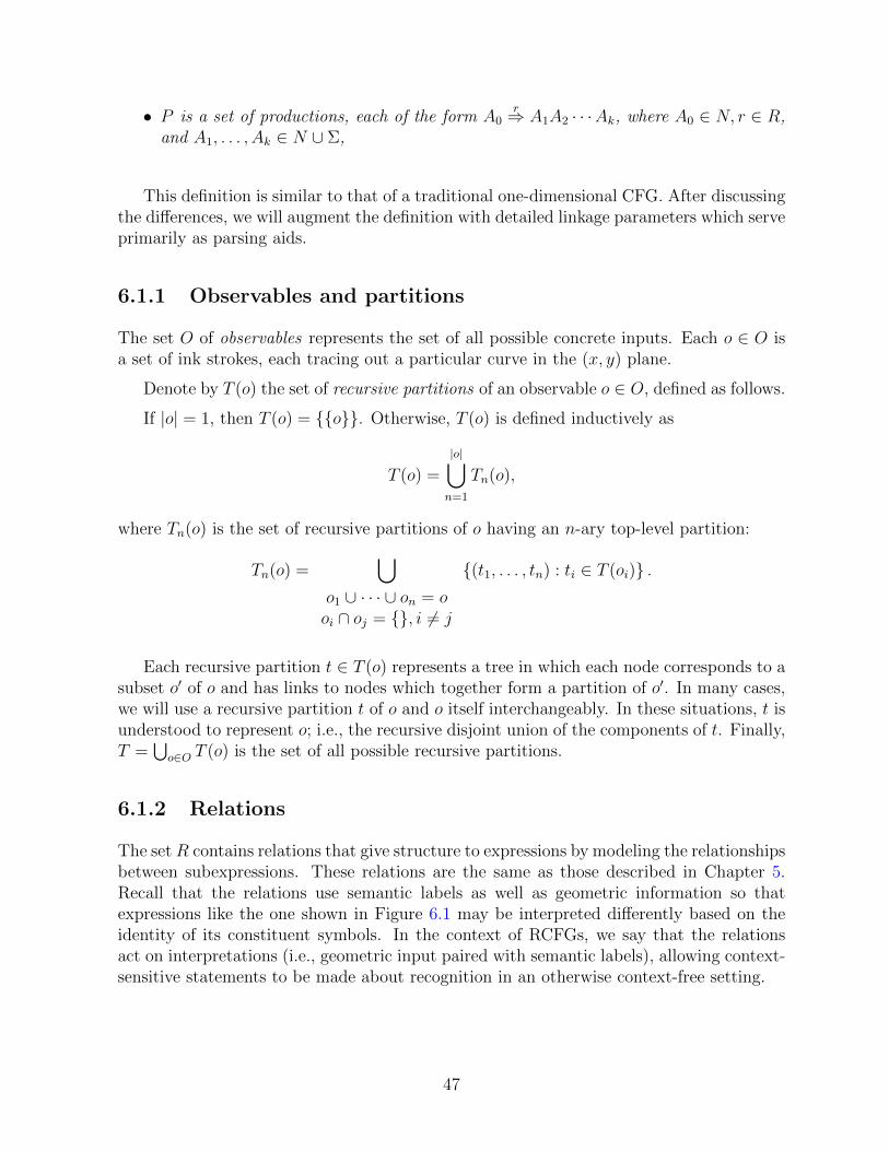
• P is a set of productions, each of the form A0r⇒ A1A2 · · ·Ak, where A0 ∈ N, r ∈ R,
and A1, . . . , Ak ∈ N ∪ Σ,
This definition is similar to that of a traditional one-dimensional CFG. After discussingthe differences, we will augment the definition with detailed linkage parameters which serveprimarily as parsing aids.
6.1.1 Observables and partitions
The set O of observables represents the set of all possible concrete inputs. Each o ∈ O isa set of ink strokes, each tracing out a particular curve in the (x, y) plane.
Denote by T (o) the set of recursive partitions of an observable o ∈ O, defined as follows.
If |o| = 1, then T (o) = {{o}}. Otherwise, T (o) is defined inductively as
T (o) =
|o|⋃n=1
Tn(o),
where Tn(o) is the set of recursive partitions of o having an n-ary top-level partition:
Tn(o) =⋃
o1 ∪ · · · ∪ on = ooi ∩ oj = {}, i 6= j
{(t1, . . . , tn) : ti ∈ T (oi)} .
Each recursive partition t ∈ T (o) represents a tree in which each node corresponds to asubset o′ of o and has links to nodes which together form a partition of o′. In many cases,we will use a recursive partition t of o and o itself interchangeably. In these situations, t isunderstood to represent o; i.e., the recursive disjoint union of the components of t. Finally,T =
⋃o∈O T (o) is the set of all possible recursive partitions.
6.1.2 Relations
The set R contains relations that give structure to expressions by modeling the relationshipsbetween subexpressions. These relations are the same as those described in Chapter 5.Recall that the relations use semantic labels as well as geometric information so thatexpressions like the one shown in Figure 6.1 may be interpreted differently based on theidentity of its constituent symbols. In the context of RCFGs, we say that the relationsact on interpretations (i.e., geometric input paired with semantic labels), allowing context-sensitive statements to be made about recognition in an otherwise context-free setting.
47

Figure 6.1: An expression in which the optimal relation depends on symbol identity.
6.1.3 Set of interpretations
While typical context-free grammars deal with strings, we call the objects derivable fromRCFGs expressions. Any terminal symbol α ∈ Σ is an expression. An expression e mayalso be formed by concatenating a number of expressions e1, . . . , ek by a relation r ∈ R.Such an r-concatenation is written e1re2r · · · rek.
The representable set of G is the set E of all expressions derivable from the nonterminalsin N using productions in P . It may be constructed inductively as follows:
For each terminal α ∈ Σ, Eα = {α}. For each production p of the form A0r⇒ A1 · · ·Ak,
Ep = {e1r · · · rek : ei ∈ EAi} .
For each nonterminal A,
EA =⋃
p∈P having LHS A
Ep.
Finally,
E =⋃A∈N
EA.
An interpretation is a pair (e, t), where e ∈ E is an expression and t is a recursivepartition in T (o) for some observable o ∈ O. An interpretation is essentially a parsetree of o where the structures of e and t encode the hierarchical structure of the parse.The set of interpretations I referenced in the RCFG definition is just the set of all theseinterpretations:
I =⋃o∈O
{(e, t) : e ∈ E, t ∈ T (o)} .
6.1.4 Productions
The productions in P are similar to context-free grammar productions in that the left-hand element derives the sequence of right-hand elements. The relation r appearing abovethe ⇒ production symbol indicates a requirement that r is satisfied by adjacent elementsof the RHS. Formally, given a production A0
r⇒ A1A2 · · ·Ak, if oi denotes an observableinterpretable as an expression ei derivable from Ai (i.e., ei ∈ EAi
and (ti, ei) ∈ I), thenfor
⋃ki=1 ti to be interpretable as (e1 r · · · r ek) requires ((ei, ti) , (ei+1, ti+1)) ∈ r for i =
1, . . . , k − 1.
48

6.2 Examples
The following examples demonstrate how RCFG productions may be used to model thestructure of mathematical writing.
1. Suppose that [ADD] and [EXPR] are nonterminals and + is a terminal. Then theproduction [ADD]
→⇒ [EXPR] + [EXPR] models the syntax for infix addition: twoexpressions joined by the addition symbol, ordered from left to right.
2. Similarly, the production [PAREN]→⇒ ([EXPR]) models the syntax for parenthesized
expressions.
3. The production [FRAC]↓⇒ [EXPR]—[EXPR] models a fraction: a numerator, fraction
bar, and denominator ordered from top to bottom.
4. The production [SUP]↗⇒ [EXPR][EXPR] models superscript syntax. Interpreted as
exponentiation, the first RHS token represents the base of the exponentiation, andthe second represents the exponent. The tokens are connected by the ↗ relation,reflecting the expected spatial relationship between subexpressions.
5. The following pair of productions models the syntax of definite integration:
[ILIMITS]↓⇒ [EXPR]
∫[EXPR]
[INTEGRAL]→⇒ [ILIMITS][EXPR]d[VAR]
Definite integrals are drawn using two writing directions. The limits of integrationand integration sign itself are written in a vertical stack, while the integration sign,integrand, and variable of integration are written from left to right.
6.3 Linkage parameters
It is often convenient to specify what portion of an expression a relation should apply to.For example, in the expression ∫ ∞
0
e−x2
dx,
we may want the → relation between the limits of integration and the integrand to applyto the symbols
∫and e, and the ↗ relation between e and its exponent to apply to e and
−x. Yet in ∫ 1
0
x2 + 1√x2 − 1
dx,
we may want the→ relation between the limits of integration and the integrand to apply tothe
∫symbol and the fraction as a whole, and the ↓ relations linking the numerator to the
49

fraction bar and the fraction bar to the denominator to apply to complete subexpressionsas well.
This flexibility is made possible by augmenting grammar productions with head, tail,and linkage parameters. Define the set S = {sym,grp,def} of linkage specifiers corre-sponding to the notions “symbol”, “group” and “default”, respectively. Then we augmentthe grammar definition by adding the following components to the tuple:
1. H : P → N is a function mapping each production to the RHS element which is itshead,
2. T : P → N is a function mapping each production to the RHS element which is itstail,
3. L : P × N → S2 is a function defining the linkage specifier at each position of eachproduction, and
4. L0 : P → S is a function specifying the parent linkage of each production.
Let p be a production A0r⇒ A1 · · ·Ak. Then p has a tail T (p) which is the RHS com-
ponent from which outgoing relations are tested, and a head H(p) which is the componentto which incoming relations are tested.
For example, in the production for addition above, we might choose the first [EXPR]
on the RHS as the expression’s head, and the second (final) [EXPR] as the expressions tail.But in the production of [ILIMITS], we might choose the integral sign as both the headand tail so that when a parse of [ILIMITS] is included in a parse of [INTEGRAL], the →relation joining the limits of integration to the integrand is tested against the integral signand not against some other part of that subexpression.
The linkage function L(p, i) gives a pair (`i, `i+1) of linkage specifiers controlling how arelation between Ai and Ai+1 should be tested. Consider a relation r ((ei, ti), (ei+1, ti+1))as being from (ei, ti) and to (ei+1, ti+1). The head and tail pointers of the productions usedto obtain those two interpretations may be followed recursively until individual symbolsare reached. These symbols are called the head and tail symbols of the expression.
The from and to components with which the relation r is queried are chosen based onthe linkage specifiers as follows:
1. If `i = sym, then the from component is given by the tail symbol of the interpretation(ei, ti). If `i+1 = sym, then the to component is given by the head symbol of theinterpretation (ei+1, ti+1).
2. If `i = grp, then the from component is the entire interpretation (ei, ti); similarly if`i+1 = grp, then the to component is the entire interpretation (ei+1, ti+1).
3. If `i = def, then the from component is selected based on the parent linkage L0(pi)of the production pi with LHS Ai used to obtain the interpretation (ei, ti). Similarly,if `i+1 = def, then the to component is selected based on the parent linkage L0(pi+1)of the production pi+1 with LHS Ai+1 used to obtain the interpretation (ei+1, ti+1).
50

The parent linkage L0(p) of a production p determines how a relation from or to anexpression derived from p is tested in the case where that expression appears as a subex-pression in some larger expression using the def linkage specifier (i.e., item 3 above). Assuch, at any given point in a parse, the parent linkage of p determines either the from orto component of a relation query, as follows:
1. If L0(p) = sym, then the tail (head) symbol of the interpretation of p is used as thefrom (to) component.
2. If L0(p) = grp, then the entire interpretation of p is used as the from (to) component.
3. If L0(p) = def, then the from (to) component is obtained recursively based on theparent linkage L0(p∗), where p∗ is the production with LHS AT (p) (AH(p)) used toobtain the interpretation of the tail (head) nonterminal of p.
By default, the head of a production A0r⇒ A1 · · ·Ak is 1 (i.e., its first RHS element)
and the tail is k (i.e., its last RHS element). If linkage parameters are not specified by thegrammar, they default to def.
6.3.1 Examples
For example, assume the following parameters for the productions in section 6.2.
• the head and tail of the [ADD] and [ILIMITS] productions are as described above,and the parent linkage of [ILIMITS] is sym;
• the parent linkage of the [FRAC] production is grp, and within the production,the linkage from [EXPR] to — is (grp, sym) and the linkage from — to [EXPR] is(sym,grp); and
• the parent linkage of [SUP] is grp, and the linkage from [EXPR] to [EXPR] withinthe production is (sym,grp).
When deriving the expected parse of the expression in Figure 6.2, relations will betested as follows:
• The ↓ relation will be tested between 1 and∫
and between∫
and 0 when parsing[ILIMITS], as usual.
• When parsing the exponential, the↗ relation will be tested between the right paren-thesis ) and the entire subexpression x2 + 1 because the relevant linkage specifier is(sym,grp), and ) is the tail symbol of the subexpression (ae).
• When parsing the fraction, the ↓ relation will be tested between the entire numerator(ae)x
2+1 and the fraction bar, and between the fraction bar and the denominator x−1because the linkage specifiers are (grp, sym) and (sym,grp), respectively.
51

Figure 6.2: An expression demonstrating a variety of subexpression linkages.
• When parsing the entire expression as [INTEGRAL], the → relation will be testedbetween the integral sign and the entire fraction. Because no explicit linkage was setbetween those two nonterminals in the [INTEGRAL] production, the default specifierwill lookup the parent linkages. For [ILIMITS], the parent linkage is sym, so thetail symbol
∫is used. For the fraction, the parent linkage is grp, so the entire
subexpression is used.
As these examples demonstrate, the linkage parameters permit very flexible yet precisecontrol over which subexpressions are selected for relation queries during parsing.
6.4 Set of interpretations as a directed set
Given a particular input observable o ∈ O, define the set of interpretations of o as thesubset of the grammar’s set of interpretations that concern o:
Io = {(e, t) ∈ I : t = o} .
It is useful to define notation for further subsets of Io matching the structure of therepresentable set of G. For cleaner notation, assume that the grammar productions are ina normal form such that each production is either of the form A0 ⇒ α, where α ∈ Σ isa terminal symbol, or of the form A0
r⇒ A1 · · ·Ak, where all of the Ai are nonterminals.This normal form is easily realized by, for each α ∈ Σ, introducing a new nonterminalXα, replacing all instances of α in existing productions by Xα, and adding the productionXα ⇒ α.
Then, for every observable o, define the following notations.
Definition 2 (Interpretations of o).
1. For every production p of the form A⇒ α, define
Ipo = {(α, t)}
for t the trivial recursive partition {o}.
52

2. For every nonterminal A, define
IAo =⋃
p having LHS A
Ipo .
3. For every production p of the form A0r⇒ A1 · · ·Ak, define
Ipo = {(e1r · · · rek, (t1, . . . , tk)) : (ei, ti) ∈ IAiti , i = 1, . . . , k;
(t1, . . . , tk) ∈ Tk(o);((ei, ti) , (ei+1, ti+1)) ∈ r, i = 1, . . . , k − 1} .
Given a scoring function sc (e, t) : I → [0, 1] on interpretations, we treat these setsof interpretations as directed sets using the preorder (e1, t1) ≤ (e2, t2) ⇐⇒ sc (e1, t1) ≤sc (e2, t2). (Recall that the preorder for a directed set is reflexive and transitive, but notnecessarily antisymmetric; that is (e1, t1) ≤ (e2, t2) and (e2, t2) ≤ (e1, t1) do not togetherimply that the two interpretations are identical.)
Using these definitions, recognizing an input o can be seen as a process which reportselements of ISo (for S the grammar’s start symbol) from greatest to least.
6.5 Semantic expression trees and textual output
RCFG productions model the two-dimensional syntax of mathematical expressions. Torepresent mathematical semantics, each production is also associated with rules for gener-ating textual output and math expression trees with semantic information. For example,consider again the production [ADD]
→⇒ [EXPR] + [EXPR]. A rule to generate a MathMLstring would be written in our grammar format as <mrow>%1<mo>+</mo>%3</mrow>, wherethe “%n” notation indicates that the string representation of the nth RHS element shouldbe inserted at that point. A rule to generate a semantic expression tree would be writtenADD(%1,%3). This rule would generate a tree with the root node labelled with additionsemantics (“ADD”) and two subtrees. Similarly to the string case, the %n notation indicatesthat the tree representation of the nth RHS element should be used as a subtree. Hence,the first child tree corresponds to the left-hand operand of the addition expression, andthe second child tree corresponds to the right-hand operand.
53

Chapter 7
Two-dimensional parsing
There are two particular properties of RCFGs that make parsing difficult. Like otherrelational grammars, the languages they generate are multi-dimensional. This prevents thestraightforward application of common parsing techniques like Earley’s algorithm, whichassume a simply ordered sequence of input tokens. Multi-dimensionality also complicatesthe task of deciding which subsets of the input may contain a valid parse. Furthermore,because our input is ambiguous, we require a parser to report all recognizable parse trees.Since there may be exponentially many trees, some effort is required to ensure a reasonablerunning time.
7.1 Shared parse forests
Each of the three recognition subsystems described in Chapters 3, 4 and 5 may introduceambiguity into parsing, reflecting the ambiguity present in the user’s handwritten input.The ambiguity takes one of three forms based on its origin:
• A particular subset of the input may or may not correspond to a distinct symbol.The output of the grouping system measures the plausibility that a given subset isin fact a symbol.
• The identity of a given symbol candidate is ambiguous. The output of the symbolrecognizer assigns scores to each possible identity.
• The spatial relationship between input subsets, whether symbols or subexpressions,is ambiguous. The output of the relation classifier assigns scores to each possibility.
Because of these ambiguities, the number of potential parses of a given input is, ingeneral, exponential in the number of input strokes. It is therefore infeasible to generateall possible parses and pick one to report to the user. This problem is similar to thatof parsing ambiguous languages, in which the same input may be represented by manyparse trees. (Indeed, the language of math expressions is ambiguous even in the absence
54

of syntactic fuzziness due to the semantic ambiguities identified in Chapter 1). Parsingambiguous languages is a well-studied problem; we adopt the shared parse forest approachof Lang [15], in which all recognizable parses are simultaneously represented by an AND-OR tree.
For example, consider the expression shown in Figure 7.1 along with the following toygrammar:
[ST]⇒ [ADD] | [TRM][ADD]
→⇒ [TRM] + [ST]
[TRM]⇒ [MUL] | [SUP] | [CHR][MUL]
→⇒ [SUP][TRM] | [CHR][TRM]
[SUP]↗⇒ [CHR][ST]
[CHR]⇒ [VAR] | [NUM][VAR]⇒ a | b | · · · | z[NUM]⇒ 0 | 1 | · · · | 9
Figure 7.1: An ambiguous mathematical expression.
Figure 7.2 depicts a shared parse forest representing some possible interpretations ofFigure 7.1. In the figure, the boxed arrows are AND nodes in which the arrows indicate therelation that links derived subexpressions. The ovals are OR nodes representing derivationsof nonterminals on particular subsets of the input. The circles relate subsets of the inputwith terminal symbols from the grammar. Simple productions of the form [CHR]⇒ [VAR],for example, have been omitted for clarity. Any tree rooted at the [ST] node that hasexactly one path to each input element is a valid parse tree. This shared parse forestcaptures, for example, the expressions Ax+ b, AX + 6, Ax + 6, AXtb, etc. If an expressionis incomplete (e.g., (x+ y without the closing parenthesis), then no parse will exist for thecorrect interpretation. However, other parses using different interpretations of the inputmay exist (e.g., lx+ y or Cxty).
Parsing an RCFG may be divided into two steps: forest construction, in which a sharedparse forest is created that represents all recognizable parses of the input, and tree extrac-tion, in which individual parse trees are extracted from the forest in decreasing score order.We describe each of these steps in turn.
55

VAR
A + tX x 6b
VAR VAR VAR NUM
MUL
→
SUP→
TRM
CHR
MUL
→
MUL
→
→MUL
→
ADD
→
ST
Figure 7.2: Shared parse forest for Figure 7.1.
56

7.2 Shared parse forest construction
Because the symbols appearing in a two-dimensional math expression cannot be simplyordered, one would naively have to parse every subset of the input in order to obtain allpossible parses. To develop a practical parsing algorithm, we introduce constraints on howthe input may be subdivided into individual symbols and subexpression so as to limit howmany input subsets must be considered. The constraints are based on the two-dimensionalstructure of mathematical notation.
7.2.1 The ordering assumption and rectangular sets
Define two total orders on observables: <x orders observables by minimum x-coordinatefrom left to right, and <y orders observables by minimum y-coordinate from top to bottom.(We take the y axis to be oriented downward.) Associate each relation r ∈ R with one ofthese orders, denoted ord r. ord r is the dominant writing direction used for a particularrelation. For math recognition, we use ord→ = ord↗ = ord↘ = ord� =<x, andord ↓ =<y.
Informally, we assume that each relation r ∈ R is embedded in either <x or <y. Thus,we may treat any grammar production as generating either horizontal or vertical concate-nations of subexpressions, making the partition-selection problem much simpler.
More formally, denote by mind t the element a ∈ t such that a <d b for all b ∈ t asidefrom a, and define maxd t similarly.
Assumption 1 (Ordering). Let t1, t2 be observables, and let e1, e2 be representable expres-sions. We assume that ((e1, t1), (e2, t2)) 6∈ r whenever maxord r t1 ≥ord r minord r t2.
The ordering assumption says that, for a parse to exist on t1 ∪ t2, the last symbol oft1 must begin before the first symbol of t2 along the dominant writing direction of theexpression being parsed. For example, in Figure 7.1, to parse Ax + b in the obvious wayrequires that the A begins before the x, and the + begins after the x but before the b,when the symbols are considered from left to right (i.e., ordered by <x).
Similarly, we could formulate a production for fractions as [FRAC]↓⇒ [EXPR]—[EXPR].
Then to parse a fraction would require that the bottom symbol of the numerator began be-fore the fraction bar, and the fraction bar began before the top symbol of the denominator,when considered from top to bottom (i.e., ordered by <y).
Liang et al. [18] proposed rectangular hulls as a subset-selection constraint for two-dimensional parsing. A very similar constraint that we call rectangular sets is implied bythe ordering assumption.
Definition 3 (Rectangular set/partition). Call a subset o′ of an observable o rectangularin o if it satisfies
o′ ={a ∈ o : min
xo′ ≤ a ≤ max
xo′}∩{a ∈ o : min
yo′ ≤ a ≤ max
yo′}.
57

Call a recursive partition t of o rectangular if every component in t is rectangular in o.
From the definition of <x and <y, a set o′ that is rectangular in o must include allstrokes from o whose left edge lies between the left-most left edge of an element in o′ andthe right-most left edge and whose top edge lies between the top- and bottom-most topedges of elements of o′.
Proposition 1. Let o ∈ O be an observable, and let p be a production of the formA0
r⇒ A1 · · ·Ak. Under the ordering assumption, if (e1r · · · rek, (t1, . . . , tk)) ∈ Ipo , thenthe recursive partition t = (t1, . . . , tk) of o is rectangular.
Proof. Let d = ord r, and choose any component ti of t. We must show that
ti ={a ∈ o : min
xti ≤x a ≤x max
xti
}∩{a ∈ o : min
yti ≤y a ≤y max
yti
}.
It is clear that ti is a subset of the RHS, so suppose that there is some a′ ∈ o in theRHS put into tj 6= ti by the partition of t. If j < i, then
((tj, ej), (tj+1, ej+1)) , . . . , ((ti−1, ei−1), (ti, ei)) ∈ r.
By the assumption,
maxdtj <d min
dtj+1 ≤ max
dtj+1 <d · · · <d min
dti.
But mind tj ≤d a′ ≤d maxd tj since a′ ∈ tj, and mind ti ≤d a′ ≤d maxd ti since a′ is in theRHS, so mind ti ≤d a′ ≤d maxd tj, a contradiction. A similar contradiction can be obtainedin the case where j > i.
Rectangular sets are the natural two-dimensional generalization of contiguous sub-strings in one-dimensional string parsing. This definition could be generalized to arbitrarydimension, giving “hypercube sets” of input elements.
Following Liang et al., notice that any rectangular set u ⊆ o can be constructed bychoosing any four strokes in o and taking them to be represent the left, right, top, andbottom boundaries of the set. There are therefore O (|o|4) rectangular subsets of o. If weinstead naively parsed every subset of the input, there would of course be 2|o| subsets toprocess. The ordering assumption thus yields a substantial reduction in the number ofsubsets that must be considered for parsing.
Liang et al. define a rectangular hull of a set of input elements to be their geometricbounding box, and they parse only those sets whose rectangular hulls have a null intersec-tion. That is, no bounding box of a subset selected for parsing can intersect that of anyother parsed set. This formulation causes problems for containment notations like squareroots, as well as for somewhat crowded or messy handwriting styles, which our rectangularset formulation avoids. For example, consider the square root expression on the left ofFigure 7.3. The rectangular hulls of the root symbol and its argument are shown as solid
58

Figure 7.3: Expressions with overlapping symbol bounding boxes.
boxes and are the (union of) geometric bounding boxes of the symbols. Note that therectangular hull of the square root symbol intersects (in fact contains) that of its contents.The argument cannot be separated from the operator into non-intersecting hulls.
When considering input subsets as rectangular sets, we do not use the natural geometricbounding box of the strokes, as Liang et al. do. Instead, we take only the minimal x andy coordinates of each stroke, and consider the bounding box (or rectangular hull) of thosepoints. The “boundary” of the root symbol in Figure 7.3 is thus the single point at thetop-left of its bounding box, and the boundary of the rectangular set representing theargument 2π is shown as a dotted box. By using minimal coordinates instead of completebounding boxes, the rectangular set boundaries do not intersect.
Similarly, in the expression on the right of Figure 7.3, the rectangular hull of openingparenthesis intersects the hull of the a symbol, and that of the closing parenthesis inter-sects the hulls of both the 3 and the exponent 2. As before, the expression cannot bepartitioned such that the required subsets’ hulls are non-intersecting. But the boundary ofthe rectangular set representing a− 3 (indicated by a dotted box) extends only to the leftedge of the 3 symbol. The boundaries of the parentheses and the exponent are, as for theroot sign, single points at the top-left corner of their bounding boxes. This small change –taking the left- and top-most coordinates of strokes as their representative points, “spacesout” overlapping writing and facilitates non-intersecting partitions.
Figure 7.4 illustrates schematically the recursive rectangular partitioning of an expres-sion, following the expected parse of
∑n−1i=1
i2
n−i . The whole expression is a rectangular set.The central dotted vertical line indicates a rectangular partition into the sum symbol (withlimits) and the summand. In the summand, for example, the two horizontal dashed linesindicate a rectangular partition into the numerator, fraction bar, and denominator, and thenumerator and denominator are further partitioned into rectangular sets, each containinga single symbol. Note that the resulting boxes in the figure are meant to emphasize thehierarchical structure of the partition. They do not indicate the geometric bounding boxesof the rectangular sets.
7.2.2 Parsing algorithms
Using the restriction to rectangular partitions derived above, we develop bottom-up andtop-down algorithms for constructing the shared parse forest of an input. The output ofeach of those techniques is a table B of parse links indexed by a nonterminal grammarsymbol A ∈ N and a rectangular subset o of the input observable. Table entry B(A, o)represents the set IAo of interpretations of A of the observable o.
59

Figure 7.4: Recursive rectangular partitions in an expression.
Bottom-up parsing
Algorithm 7 generalizes to two dimensions the well-known CYK algorithm for CFG parsing.It uses dynamic programming to parse each rectangular subset of the input from smallestto largest. As in the CYK algorithm, the grammar is assumed to be in Chomsky NormalForm. That is, each production is either of the form A0 ⇒ α for some α ∈ Σ, or of theform A0
r⇒ A1A2, where r ∈ R and B,C ∈ N .
Algorithm 7 Bottom-up RCFG parser.
Require: An input observable o.for every rectangular subset o′ ⊂ o of size |o′| = 1, 2, . . . , |o| do
for each production p of the form A⇒ α doif o′ is recognizable as α by the symbol recognizer thenB(A, o′)← B(A, o′) ∪ {(p; (o′))}
for each production p of the form A0r⇒ A1A2 do
d← ord rfor x ∈ (o′ \ {mind o
′}) doo1 ← {a ∈ o′ : a <d x}o2 ← {a ∈ o′ : a ≥d x}if B(A1, o1) 6= {} and B(A2, o2) 6= {} thenB(A, o′)← B(A, o′) ∪ {(p; (o1, o2))}
Any rectangular subset of an observable o may be constructed by following Algorithm8. We can thus pre-compute all rectangular subsets of o so that they are accessible toAlgorithm 7 in constant time. This precomputation step requires O (|o|5 log |o|) operationsusing standard sorting techniques. The algorithm proper requires O (|P ||o|) operations perrectangular subset, for a total runtime of O (|o|5 (|P |+ log |o|)).
Top-down parsing
The bottom-up parsing algorithm above is straightforward but has two downsides. First,the requirement to re-write the grammar in Chomsky normal form complicates the imple-mentation of linkage parameters in the grammar. By re-organizing the productions, the
60

Algorithm 8 Rectangular subset extraction.
Let d be one of x, y and let d′ be the other.List the elements of o in increasing order under <d.Extract a contiguous subsequence. (We now have a set o′ ⊆ o satisfying o′ ={a ∈ o : mind o
′ ≤d a ≤d maxd o′}.)
Re-order the remaining elements into increasing order under <d′ .Extract a contiguous subsequence. (The subsequence elements comprise a rectangularsubset of o.)
correspondence between non-terminals and input subsets is changed – the group of strokesreferred to by a grp linkage parameter in the CNF grammar may be different from thegroup referred to by the same parameter in the original grammar. Second, experimentswith the CYK approach showed that, while all rectangular sets must be enumerated andparsed, relatively few actually contribute to valid parse trees. A similar observation wasmade by Grune and Jacobs [10] in the case of ambiguous languages. The algorithm’sruntime, while predictable, is always the worst-case time.
Instead of CYK, we therefore adapted to RCFGs a tabular variant of Unger’s methodfor CFG parsing [33]. In this approach, we assume that the grammar is in the normal formdescribed in Section 6.4. At a high level, the algorithm parses a production p on an inputsubset o as follows:
1. If p is a terminal production, A0 ⇒ α, then check if o is recognizable as α accordingto the symbol recognizer. If it is, then add the parse link (p; (o)) to table entryB(A0, o); otherwise parsing fails.
2. Otherwise, p is of the formA0r⇒ A1 · · ·Ak. For every rectangular partition (t1, . . . , tk)
of o, parse each nonterminal Ai on ti. If any of the sub-parses fail, then fail on thecurrent partition. Otherwise, add (p; (t1, . . . , tk)) to table entry B(A0, o). If parsingfails on every partition, then parsing fails on o.
One drawback of this algorithm is that its runtime is exponential in the size of theRHS of a grammar production, since case 2 above iterates over
( |o|k−1
)partitions. This
bound is obtained by sorting the input by <ord r and choosing k−1 split points to induce arectangular partition. In the worst case, then (i.e., when parses exist on every partition),our algorithm must consider every grammar production on every rectangular set, giving acomplexity of O
(n3+kpk log n
), where n is the number of elements in the input observable,
p is the number of grammar productions, and k is the number of RHS tokens in the largestproduction. The extra factor of k arises from writing up to k partition subsets into a parsetable entry in case 2 above. Importantly, k can be controlled by the designer of a grammaras a tradeoff between RHS size and number of grammar productions. For example, if thegrammar is written in Chomsky Normal Form (CNF), then the complexity is O (n5p). Notethat the general bound is asymptotically tight to the worst-case size of the parse forest,since there may be O (n4p) table entries (counting each production as a distinct entry),each of which may link to O
(nk−1k
)other table entries.
61

Instead of writing our grammar in CNF, we allow arbitrary production lengths anduse the following three optimizations to reduce the number of partitions that must beconsidered. The first two are typical when using Unger’s method [10]; the third is specificto fuzzy r-CFG parsing.
1. Terminal symbol milestones. The symbol recognizer may be used to guide parti-tioning. Suppose p is A0
r⇒ A1 · · ·Ai−1αAi+1 · · ·Ak, where α is a terminal symbol.Then for a parse to exist on the partition (t1, . . . , tk), the symbol α must have beenreported as a candidate for the subset ti. In general, given a partition, any subsetcorresponding to a terminal symbol in the grammar production must be recognizableas that terminal symbol. We therefore “seed” the parse table with symbol recogni-tion results, and limit the enumeration of rectangular partitions to those for whichthe appropriate terminal symbols are already present in the parse table. Such seed-ing also facilitates recognition of typeset symbols, which are simply inserted into theparse table with their known identities prior to invocation of the parsing algorithm.
2. Minimum nonterminal length. If there are no empty productions in the grammar,then each nonterminal must expand to at least one terminal symbol. Moreover, givena minimum number of strokes required to recognize a particular symbol (e.g., at leasttwo strokes may be required to form an F ), one can compute the minimal numberof input elements required to parse any sequence of nonterminals A1 · · ·Ak. Thesequantities further constrain which partitions are feasible.
For example, consider the expression in Figure 7.1. Suppose we are parsing theproduction [ADD]
→⇒ [TRM] + [ST] and we know that the + symbol must be drawnwith exactly two strokes. Then [ADD] cannot be parsed on fewer than 4 input strokes,and the input must be partitioned into subsets t1, t2, and t3 such that |t1| ≥ 1, |t2| =2, |t3| ≥ 1. Furthermore, from the previous optimization, t2 must be chosen suchthat it is recognizable as the symbol +. In this particular case, only one partition isfeasible.
3. Spatial relation test. Just because an input subset can be partitioned into rectangularsets does not mean that those sets satisfy the geometric relations specified by agrammar production. Unfortunately, the grammar relations act on expressions aswell as observables, so they cannot be tested during parsing because expressionsare not explictly constructed. As there may be exponentially many expressions,they cannot be constructed, and therefore we cannot evaluate the grammar’s spatialrelations, which vary with expression identity. Still, we can speed up parsing bytesting whether relations are satisfied which approximate the grammar relations.
Namely, we use the rule-based relation classifier described in Section 5.1 with seman-tic labels both set to the generic label gen. If the classifier reports a score of zerowhen tested on adjacent partition subsets ti and ti+1, then the entire partition isdiscarded. The rule-based variant is not as accurate as the other relation classifiers,but it is fast to compute and accepts inputs with a wide variance of features. Forthis filtering stage, it is better to accept false positives than to reject false negatives.
62

In the algorithms below, we denote by r the rule-based relation corresponding togrammar relation r.
Parsing a production A0r⇒ A1 · · ·Ak on an observable o proceeds by two mutually
recursive procedures. The first procedure, Parse-Nt-Seq, parses a sequence A1 · · ·Ak ofnonterminals on an observable o, as follows:
1. If k = 1, then parse the nonterminal A1 on o. Fail if this sub-parse fails.
2. Otherwise, for every rectangular partition of o into two subsets, o1 and o2, such that|o1| ≥ minlen(A1) and |o2| ≥ minlen(A2 · · ·Ak), parse A1 on o1, and recursivelyparse the nonterminal sequence A2 · · ·Ak on o2. Fail if either parse fails.
The second procedure, Parse-Seq, parses a general sequence A1 · · ·Ak of nonterminalsand terminals on o, as follows. Let d = ord r, and let i be minimal such that Ai is a terminalsymbol. Then each rectangular o′ ⊆ o that is recognizable as Ai according to the symbolrecognizer induces a rectangular partition of o into o1, o
′, o2, where maxd o1 <d mind o′ and
maxd o′ <d mind o2. For each of these partitions satisfying |o1| ≥ minlen(A1 · · ·Ai−1) and
|o2| ≥ minlen(Ai+1 · · ·Ak), parse A1 · · ·Ai−1 on o1, and parse Ai+1 · · ·Ak on o2. Fail ifeither sub-parse fails.
So, to parse a production, we just check whether its RHS contains terminals or not,and invoke the appropriate procedure. To clarify the outline of the algorithm, we haveomitted the relational tests described in optimization 3 above. These details are includedin the pseudocode below.
Algorithm 9 Parse-Nt-Seq: Top-down parser for nonterminal sequences.
Require: A sequence A1 · · ·Ak of nonterminal symbols, a set o of input strokes, a grammarrelation r, a leading set oL, and a trailing set oR.B′ ← {}d← ord rif k = 1 then
(Verify that o fits in via r with the leading and trailing sets)if ((oL, o) ∈ r or oL = {}) and ((o, oR) ∈ r or oR = {}) then
return Parse(A1, o)for L = minlen(A1), . . . , |o| −minlen(A2 · · ·Ak) do
Let o1 ⊆ o be the first L elements of o ordered by <d.if (oL, o1) ∈ r or oL = {} thenB1 ← Parse(A1, o1)if B1 6= {} thenB2 ← Parse-Nt-Seq(A2 · · ·Ak, o \ o1, r, o1, oR)B′ ← B′ ∪ {b1, b2 : b1 ∈ B1, b2 ∈ B2}
return B′
These functions comprise the two-dimensional parsing algorithm that we use in practicefor MathBrush. Each production A0
r⇒ A1 · · ·Ak is parsed recursively by parsing A2 · · ·Ak
63

Algorithm 10 Parse-Seq: Top-down parser for general production sequences.
Require: A sequence A1 · · ·Ak of grammar symbols from N ∪Σ, a set o of input strokes,a grammar relation r, and a leading set oL.Let i be minimal such that Ai is a terminal symbolB′ ← {}d← ord rfor every rectangular subset o′ of o recognizable as the terminal symbol Ai doo1 ← {a ∈ o : a <d mind o
′}o2 ← {a ∈ o : maxd o
′ <d a}if minlen(A1 · · ·Ai−1) ≤ |o1| and minlen(Ai+1 · · ·Ak) ≤ |o2| thenB1 ← Parse-Nt-Seq(A1 · · ·Ai−1, o1, r, oL, o
′)if at least one of Ai+1, . . . , Ak is a terminal symbol thenB2 ← Parse-Seq(Ai+1 · · ·Ak, o2, r, o
′)elseB2 ← Parse-Nt-Seq(Ak+1 · · ·Ak, o2, r, o
′, {})B′ ← B′ ∪ {b1, o
′, b2 : b1 ∈ B1, b2 ∈ B2}return B′
Algorithm 11 Parse: Top-down parser entry point.
Require: A nonterminal A0 and a set o of input strokes.if B(A0, o) is not marked “parsed” then
for each production p of the form A0r⇒ A1 · · ·Ak do
if at least one of A1, . . . , Ak is a terminal symbol thenB′ ← Parse-Seq(A1 · · ·Ak, o, r, {})
elseB′ ← Parse-Nt-Seq(A1 · · ·Ak, o, r, {}, {})
Mark B(A0, o) “parsed”B(A0, o)← {(p;x) : x ∈ B′}
return B′
for each valid subset choice for A1, aborting a recursive branch when no valid subset choicesexist. This approach may be seen as a depth-first search in the space of valid partitions.But the optimizations described above constraint the search space and significantly speedup the parsing process. The technique is fast enough that recognition results may beupdated and displayed in real-time as the user is writing.
7.3 Extracting interpretations
Recall from Chapter 6 that ISo is the set of interpretations of an observable o with respectto a given RCFG. Our goal is to extract elements of ISo and report them to the user indecreasing score order. The parse forest constructed using the algorithms in the previoussection is a representation of ISo from which individual parse trees, each corresponding toan interpretation, may be extracted. In this section, we develop algorithms for performing
64

this tree extraction task efficiently.
7.3.1 The monotone assumption
Define the rank of an element x of a directed set (X,≤) as the number of elements y ∈ Xsuch that x ≥ y. Applying this definition to the set ISo of interpretations, with ≤ defined interms of the scoring function sc as described in Section 6.4, the top-scoring interpretationwill have rank 1, the interpretation with second highest score will have rank 2, and so on.Denote the element of a directed set X with rank n by [n]X.
Consider the problem of finding [1]Ipo , the highest-ranked parse of a production p on theobservable o. Supposing, as usual, that p has the form A0
r⇒ A1 · · ·Ak, every interpretation(e, t) in Ipo includes t a recursive partition (t1, . . . , tk) of o and e an r-concatenation of theform e1r · · · rek, where each subexpression ei is an element [mi]I
Aiti for some mi. Since we
have not constrained how sc (e, t) is calculated, the only way to determine [1]Ipo is to iterateover all combinations of mi and find the highest-scoring expression.
This exhaustive algorithm is impractical. To develop a tractable algorithm, we mustconstrain the behaviour of the scoring function. Its exact structure will be detailed inthe next chapter, but for now we assume that the score of a terminal interpretation is afunction of a symbol recognition score S(α, o) related to recognizing the observable o as αand some stroke grouping score G(o) giving the plausibility that o constitutes a symbol:
sc (α, t) = g (S (α, o) , G(o)) ,
for t the trivial partition {o} of o.
Similarly, the score of interpreting the recursive partition t = (t1, . . . , tk) as the r-concatenation e = e1r · · · rek is assumed to be a function of symbol recognition, strokegrouping, and relation classification scores, decomposable as
sc (e, t) = fk (sc (e1, t1) , . . . , sc (ek, tk) , Rr ((e1, t1), (e2, t2)) , . . . , Rr ((ek−1, tk−1), (ek, tk))) ,
where Rr(a, b) is a scoring function for the relation r applied to the interpretations a andb.
Given this assumption on the general structure of sc, we further assume that the com-bination functions g and fi increase monotonically with their arguments, subject to someconstraints. Let c`(e) denote the semantic label associated with an expression e. (Recallfrom Chapter 5 that the semantic labels group together symbols with similar bounding-boxprofiles.)
Assumption 2 (Monotone). Assume
1. If S (t, β) > S (t, α), then g (S (t, β) , G(t)) > g (S (t, α) , G(t)).
2. If c`(e1) = c`(e′1) and c`(e2) = c`(e′2), then Rr ((t1, e1), (t2, e2)) = Rr ((t1, e′1), (t2, e
′2)).
65

3. If sc (ti, ei) ≥ sc (ti, e′i) and c`(ei) = c`(e′i) for i = 1, . . . , k, then
fk (sc (t1, e1) , . . . , sc (tk, ek) , Rr ((t1, e1), (t2, e2)) , . . . , Rr ((tk−1, ek−1), (tk, ek))) ≥fk(sc (t1, e
′1) , . . . , sc (tk, e
′k) , Rr ((t1, e
′1), (t2, e
′2)) , . . . , Rr
((tk−1, e
′k−1), (tk, e
′k))).
7.3.2 Extracting elements of ISo
Using the monotone assumption, we develop an algorithm for extracting elements of ISoin rank order. The basic idea of our algorithm is to first extract the most highly-rankedexpression, [1] ISo , and then to recursively maintain an expanding “frontier” of potentialnext-best expressions, from which subsequent expressions are obtained.
In the following, we use the following refinements of the sets of interpretations in Defi-nition 2. For each nonterminal A and semantic label c, let IAo (c) =
{(e, t) ∈ IAo : c`(e) = c
}restrict IAo to expressions with label c. For a recursive partition t ∈ T (o), let Ipt ={(e, t) : (e, t) ∈ Ipo} restrict Ipo to interpretations using the partition t. Finally, for semanticlabels c1, . . . , ck, let Ipt (c1, . . . , ck) = {(e1r · · · rek, t) ∈ Ipt : c`(ei) = ci, i = 1, . . . , k} restrictIpt to interpretations in which each subexpression has a particular semantic label.
Number the semantic labels derivable from A0 as c1, . . . , cN . It is clear that [1]IA0o =
argmax{
sc(e) : e = [1]IA0o (ci), i = 1, . . . , N
}. Suppose we have determined [j]IA0
o up toj = n, yielding a partial set of expressions I =
{[j]IA0
o : j = 1, . . . , n}
. Then [n+ 1] IA0o is
given by the following result.
Proposition 2. Let I =⋃i
{[j] IA0
o (ci) : 1 ≤ j ≤ ni}
. That is, the ni most highly-rankedelements of each IA0
o (ci) have already been extracted from IA0o . Then
[n+ 1]IA0o = argmax
{sc(e) : e = [ni + 1]IA0
o (ci), i = 1, . . . , N}.
In this proposition, the indices ni represent the expanding frontier of potential next-bestexpressions. The actual next-best expression is just the best expression from the frontier.After extraction, the frontier must be updated by incrementing the appropriate ni.
Expressions may be extracted in ranked order from the set Ipo by similarly maximizingover a frontier of potential “next-best” expressions, based on the initial maximizations
[1]Ipo = argmax {sc(e) : e = [1]Ipt , t ∈ Tk(o)}
and
[1]Ipt = argmax {sc(e) : e = [1]Ipt (c1, . . . , ck); c1, . . . , ck are semantic labels} .
However, this strategy must be generalized somewhat to extract expressions from thesets Ipt (c1, . . . , ck). For brevity, we denote an r-concatenation [n1] IA1
t1 (c1)r · · · r [nk] IAktk
(ck)in a given set Ipt (c1, . . . , ck) by its indices as (n1, . . . , nk).
66
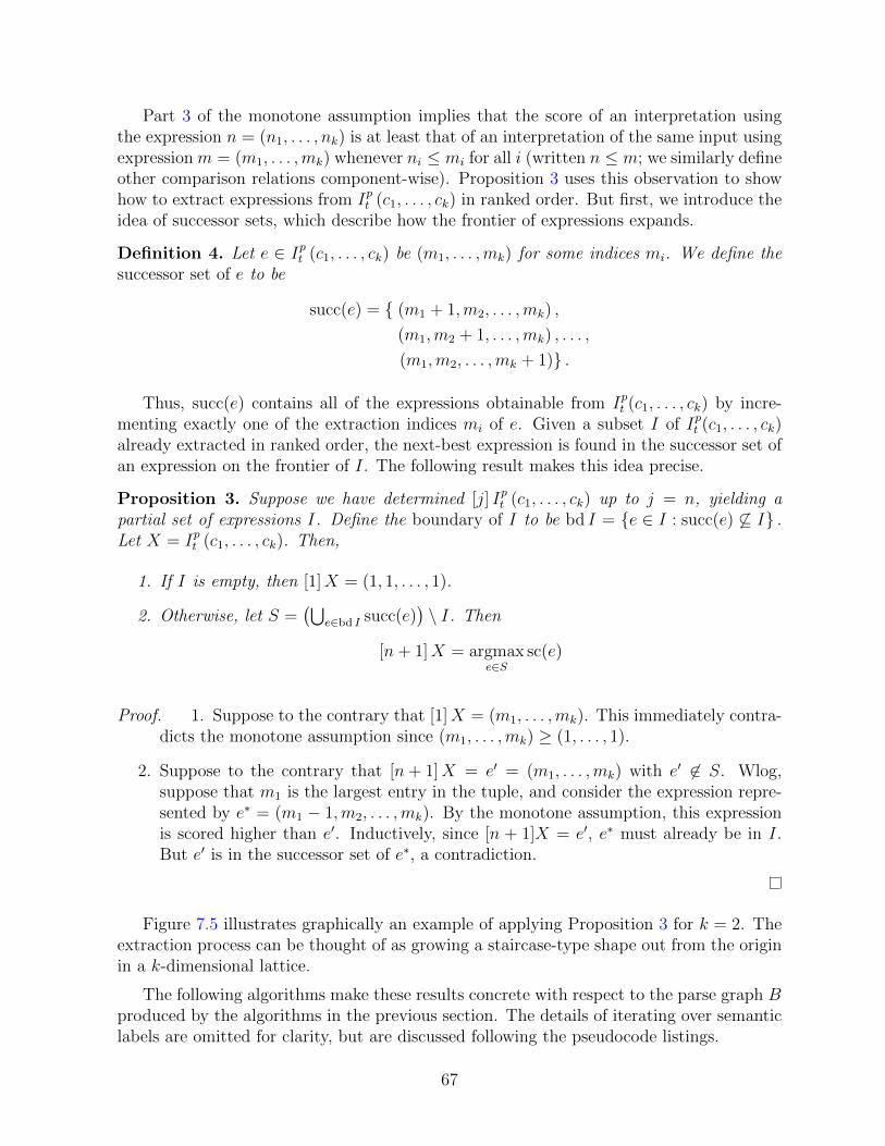
Part 3 of the monotone assumption implies that the score of an interpretation usingthe expression n = (n1, . . . , nk) is at least that of an interpretation of the same input usingexpression m = (m1, . . . ,mk) whenever ni ≤ mi for all i (written n ≤ m; we similarly defineother comparison relations component-wise). Proposition 3 uses this observation to showhow to extract expressions from Ipt (c1, . . . , ck) in ranked order. But first, we introduce theidea of successor sets, which describe how the frontier of expressions expands.
Definition 4. Let e ∈ Ipt (c1, . . . , ck) be (m1, . . . ,mk) for some indices mi. We define thesuccessor set of e to be
succ(e) = { (m1 + 1,m2, . . . ,mk) ,
(m1,m2 + 1, . . . ,mk) , . . . ,
(m1,m2, . . . ,mk + 1)} .
Thus, succ(e) contains all of the expressions obtainable from Ipt (c1, . . . , ck) by incre-menting exactly one of the extraction indices mi of e. Given a subset I of Ipt (c1, . . . , ck)already extracted in ranked order, the next-best expression is found in the successor set ofan expression on the frontier of I. The following result makes this idea precise.
Proposition 3. Suppose we have determined [j] Ipt (c1, . . . , ck) up to j = n, yielding apartial set of expressions I. Define the boundary of I to be bd I = {e ∈ I : succ(e) 6⊆ I} .Let X = Ipt (c1, . . . , ck). Then,
1. If I is empty, then [1]X = (1, 1, . . . , 1).
2. Otherwise, let S =(⋃
e∈bd I succ(e))\ I. Then
[n+ 1]X = argmaxe∈S
sc(e)
Proof. 1. Suppose to the contrary that [1]X = (m1, . . . ,mk). This immediately contra-dicts the monotone assumption since (m1, . . . ,mk) ≥ (1, . . . , 1).
2. Suppose to the contrary that [n+ 1]X = e′ = (m1, . . . ,mk) with e′ 6∈ S. Wlog,suppose that m1 is the largest entry in the tuple, and consider the expression repre-sented by e∗ = (m1 − 1,m2, . . . ,mk). By the monotone assumption, this expressionis scored higher than e′. Inductively, since [n + 1]X = e′, e∗ must already be in I.But e′ is in the successor set of e∗, a contradiction.
Figure 7.5 illustrates graphically an example of applying Proposition 3 for k = 2. Theextraction process can be thought of as growing a staircase-type shape out from the originin a k-dimensional lattice.
The following algorithms make these results concrete with respect to the parse graph Bproduced by the algorithms in the previous section. The details of iterating over semanticlabels are omitted for clarity, but are discussed following the pseudocode listings.
67

After 1 extraction After 2 extractions After 7 extractions
n1
n2
Successor set
Extracted
Not yet considered
Legend
Figure 7.5: Illustration of expression extraction for a two-token production.
We divide the problem into two parts: extracting interpretations from a particularbranch (p; (t1, . . . , tk)), and extracting interpretations from a nonterminal node B(A, o).These two parts are implemented as mutually-recursive procedures invoked according tothe structure of the grammar productions.
Algorithms 12 and 14 implement the first part, while Algorithms 13 and 15 implementthe second part. They essentially translate the consequences of the monotone assumptioninto parse graph operations. Note that each algorithm uses data structures local to thepoint in B from which it is extracting expressions. One can think of these algorithms asbeing associated directly with each node and branch in the parse graph. The process isinitialized by calling Best-Nonterminal-Expression(S, o) with S the start symbol ando the entire input. Next-Nonterminal-Expression(S, o) may then be called repeatedlyto iterate over all parses of o.
Furthermore, two distinct modes of extraction are supported. In the exhaustivemode, expressions are extracted exactly as suggested by the monotone assumption. How-ever, this leads to an overwhelming number of expressions being available to the user. Asecond mode, called semantics, is more restrictive, and is the default mode for expressionslarger than a single terminal symbol.
In semantics mode, all reported expressions must either be derived from differentproductions (and thus represent different parse structures), or, if derived from the sameproduction, must partition the input differently into subexpressions. This restriction ef-fectively constrains the number of alternatives available, while still allowing all possibleparse results to be obtained by examining the alternatives for different subexpressions. Itis easily implemented by extracting only one expression per branch.
It is difficult to precisely quantify the complexity of these algorithms. However, we cancharacterize them in terms of the size of B. The initialization step, yielding [1]It, followsevery possible branch in B(S, t) for S the start symbol and t the entire input, visitingeach node once. Extracting [n + 1]It entails a visit to only one branch per nonterminalvisited, but to k nonterminals per branch (p; (t1, . . . , tk)) visited, where k is the numberof RHS tokens in the production p. Note, though, that each such token corresponds to a
68

Algorithm 12 Best-Link-Expression: Extract the most highly-ranked expression froma branch.Require: A branch (p; (t1, . . . , tk))cache← {} (Initialize priority queue local to the branch)if p is a terminal production A0
r⇒ α thene∗ ← α
else(p is of the form A0
r⇒ A1 · · ·Ak)for i = 1, . . . , k doei ← Best-Nonterminal-Expression(Ai, ti)
e∗ ← (e1r · · · rek)[0] Ipt1∪···∪tk ← e∗
return e∗
Algorithm 13 Next-Link-Expression: Extract the next most highly-ranked expressionfrom a branch.Require: A branch (p; (t1, . . . , tk))
if extraction mode is semantics thenreturn NONE
if p is a terminal production A0r⇒ α then
return NONE(p is of the form A0
r⇒ A1 · · ·Ak)Suppose n expressions have already been extracted from this branch.Let (e1r · · · rek) = [n] Ipt1∪···∪tk be the last expression extracted here
Let mi be such that ei = [mi] IAiti for i = 1, . . . , l
for i = 1, . . . , k doif mi = |Iti | thenei ← Next-Nonterminal-Expression(Ai, ti)
elseei ← [mi + 1] IAi
ti
Add e = (e1r · · · rei−1reirei+1r · · · rek) to cache with priority Ipt (e)if cache is empty then
return NONEPop e∗ from cache[n+ 1] Ipt1∪···∪tk ← e∗
return e∗
69

Algorithm 14 Best-Nonterminal-Expression: Extract the most highly-ranked ex-pression derivable from a nonterminal.
Require: A nonterminal A and an observable t.cache← {} Initialize priority queue local to (A, t)for every branch (p;x) ∈ B(A, t) do
Add e = Best-Link-Expression(p;x) to cache with priority Ipt (e)Pop e∗ from cache[0] IAt ← e∗
return e∗
Algorithm 15 Next-Nonterminal-Expression: Extract the next most highly-rankedexpression derivable from a nonterminal.
Require: A nonterminal A and an observable t.Suppose n expressions have already been extracted from B(A, t).Let e = [n] IAt be the last expression extracted hereLet (p; (t1, . . . , tk)) be the branch from which e was extractedAdd e = Next-Link-Expression (p; (t1, . . . , tk)) to cache with priority Ipt (e)if cache is empty then
return NONEPop e∗ from cache[n+ 1] IAt ← e∗
return e∗
subexpression in the parse. The amount of work performed in this case is therefore directlyproportional to the number of nodes in a parse tree representing [n]It.
To include semantic labels in these algorithms requires some modifications of Algo-rithms 12 and 13. Whenever a terminal expression is extracted by a recursive call in oneof the algorithms (say from the nonterminal A on the trivial recursive partition t), thatrecursive call is repeated to extract all of the terminal interpretations of A on t. All theinterpretations arising from those extractions are added to the priority queue. In this way,all combinations of semantic labels are accounted for. Because of this exhaustive extrac-tion of terminal expressions, the first part of the monotone assumption is unnecessary inpractice.
In the worst case, if all possible combinations of labels are populated, this adds anadditional factor of Ck to the complexity of the tree extraction algorithm, where C is thenumber of semantic labels and k is the number of RHS elements of p. Importantly, bothC and k are controlled by the grammar designer. Furthermore, recall that only differentterminal symbols are given meaningfully different semantic labels; all larger expressionshare the generic labels expr and gen. This restriction is important because it limits thisextra iteration to only those expressions directly involving terminal symbols (i.e., near theleaves of the parse forest). No extra iteration is invoked for larger expressions because theydo not possess any non-trivial semantic labels.
The restriction of semantic labels to terminal expressions also simplifies data organi-
70
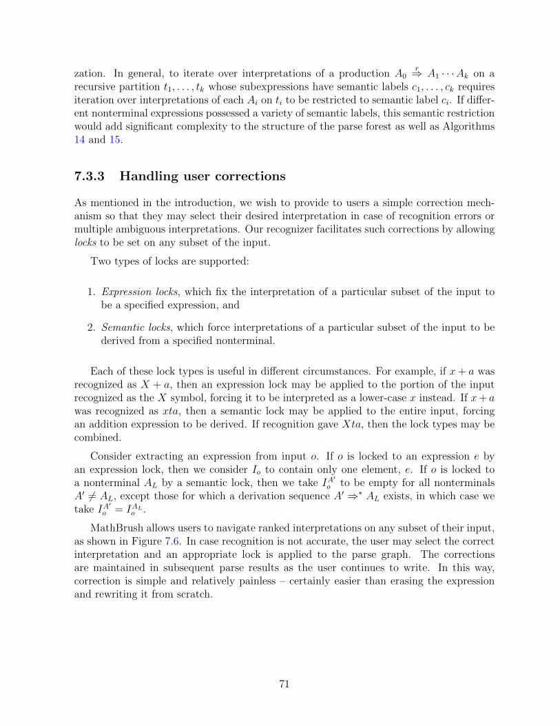
zation. In general, to iterate over interpretations of a production A0r⇒ A1 · · ·Ak on a
recursive partition t1, . . . , tk whose subexpressions have semantic labels c1, . . . , ck requiresiteration over interpretations of each Ai on ti to be restricted to semantic label ci. If differ-ent nonterminal expressions possessed a variety of semantic labels, this semantic restrictionwould add significant complexity to the structure of the parse forest as well as Algorithms14 and 15.
7.3.3 Handling user corrections
As mentioned in the introduction, we wish to provide to users a simple correction mech-anism so that they may select their desired interpretation in case of recognition errors ormultiple ambiguous interpretations. Our recognizer facilitates such corrections by allowinglocks to be set on any subset of the input.
Two types of locks are supported:
1. Expression locks, which fix the interpretation of a particular subset of the input tobe a specified expression, and
2. Semantic locks, which force interpretations of a particular subset of the input to bederived from a specified nonterminal.
Each of these lock types is useful in different circumstances. For example, if x+ a wasrecognized as X + a, then an expression lock may be applied to the portion of the inputrecognized as the X symbol, forcing it to be interpreted as a lower-case x instead. If x+ awas recognized as xta, then a semantic lock may be applied to the entire input, forcingan addition expression to be derived. If recognition gave Xta, then the lock types may becombined.
Consider extracting an expression from input o. If o is locked to an expression e byan expression lock, then we consider Io to contain only one element, e. If o is locked toa nonterminal AL by a semantic lock, then we take IA
′o to be empty for all nonterminals
A′ 6= AL, except those for which a derivation sequence A′ ⇒∗ AL exists, in which case wetake IA
′o = IAL
o .
MathBrush allows users to navigate ranked interpretations on any subset of their input,as shown in Figure 7.6. In case recognition is not accurate, the user may select the correctinterpretation and an appropriate lock is applied to the parse graph. The correctionsare maintained in subsequent parse results as the user continues to write. In this way,correction is simple and relatively painless – certainly easier than erasing the expressionand rewriting it from scratch.
71

Figure 7.6: Interface for displaying and selecting alternative interpretations.
72

Chapter 8
Scoring interpretations
The previous chapter described how a scoring function on interpretations, sc(e, t), maybe used to efficiently organize and report all parses of an input observable in order ofdecreasing score. The algorithms we developed assumed that sc was either:
1. A function sc (α, t) = g (S (α, t) , G(t)) of underlying symbol and stroke groupingscore functions for a terminal expression α, or
2. A function
sc (e1r · · · rek, (t1, . . . , tk)) = fk ( sc (e1, t1) , . . . , sc (ek, tk) ,
Rr ((e1, t1), (e2, t2)) , . . . , Rr ((ek−1, tk−1), (ek, tk)))
of sub-interpretation scores and a relation scoring function, in the general case.
In either case, we require the combination functions g and fk to be monotonic increasingin all of their arguments, as described in the previous chapter.
In this chapter, we develop two concrete scoring functions satisfying these assumptions,respectively based on fuzzy logic and probability theory. In the next chapter, the systemsresulting from combining these scoring functions with the parsing techniques described pre-viously will be evaluated and compared with an earlier version of the MathBrush recognizeras well as other recognition systems.
8.1 Fuzzy logic-based scoring
In the fuzzy case, we treat the set Io of interpretations of o as a fuzzy set, and treat sc as itsmembership function. Although the classical membership function for conjunctive variablecombinations (e.g., “the strokes of o correspond to a symbol and represent the symbol α”)is the min function, Zhang et al [41] found that using multiplication when computing
73

membership grades helped to prevent ties. We therefore compute the membership gradein the terminal case as
sc (α, t) =√S (α, o)G(t),
where S (α, o) = Dα(o)−2 for Dα the hybrid symbol distance function from Equation 4.7,and G(t) is the stroke grouping score from Chapter 3.
In the general case of an r-concatenation, we compute the membership grade as
sc (e1r · · · rek, (t1, . . . , tk)) =
((k∏i=1
sc (ei, ti)
)(k−1∏i=1
µr ((ei, ti) , (ti+1, ei+1))
)) 12k−1
,
where µr is the membership function from Section 5.1 treating each relation r as fuzzy.
The geometric averaging used in these scoring functions preserves the tie-breaking prop-erties of multiplication while normalizing for expression size.
8.2 Probabilistic scoring
The probabilistic case requires significantly more care to develop than the fuzzy case. Noneof the underlying scoring functions described above naturally produce probability distri-butions, so some transformation of those functions is required. However, probabilisticformalisms do offer straightforward and systematic ways in which to represent “common-sense” information such as symbol and subexpression co-occurrence frequencies (e.g., pre-ferring sin over sjn), and we wish to include such details in our model.
8.2.1 Model structure
Given an input observable o ∈ O, we define the following families of variables:
• An expression variable Eo ∈ {e : (e, t) ∈ Io for some t} ∪ {nil} from the set of inter-pretations of each o ⊆ o. Eo = nil indicates that the subset o has no meaningfulinterpretation.
• A symbol variable So ∈ Σ ∪ {nil} for each o ⊆ o indicating what terminal symbolo represents. So = nil indicates that o is not a symbol. (o could be a largersubexpression, or could have Eo = nil as well.)
• A relation variable Ro1,o2 ∈ R ∪ {nil} indicating which grammar relation joins thesubsets o1, o2 ⊂ o. Ro1,o2 = nil indicates that the subsets are not directly connectedby a relation.
• A vector of grouping-oriented features go for each o ⊆ o.
• A vector of symbol-oriented features so for each o ⊆ o.
74

• A vector of relation-oriented features fo for each o ⊂ o.
• A “symbol-bag” variable Bo distributed over Σ ∪ {nil} for each o ⊆ o.
This is a large group of variables: there are 22|o| relation variables alone! Fortunately,we may restrict ourselves to variable assignments which correspond to valid parse trees,which significantly reduces the model’s complexity through the following deterministicconstraints.
• The set of subsets {o : Eo 6= nil} with non-nil expressions must correspond exactlyto a recursive partition of o, otherwise the expressions do not combine to form aparse tree.
• If Eo = nil, then So = nil, and all Ro,∗ and R∗,o are also nil.
• Eo is a terminal expression iff So 6= nil.
Additionally, the ordering assumption of Section 7.2.1 allows us to also specify Eo = nilif o is not a rectangular set. This immediately reduces the number of potential non-nilexpression variables to O(|o|4) and the number of relation variables to O(|o|8).
That is still a considerable number of variables, though, so direct assessment of the jointdistribution is infeasible. Instead, we rely on the algorithms from the previous chapter topropose parse trees. Each parse tree corresponds to an assignment to the capitalizedvariables defined above in which the constraints just given are known to be satisfied. Wecompute a score for each such assignment that is proportional to the joint probability
P
(∧o⊆o
Eo,∧o⊆o
So,∧
o1,o2⊂o
Ro1,o2 ,∧o⊆o
go,∧o⊆o
so,∧o⊂o
fo,∧o⊆o
Bo
).
To do so, first factor the joint distribution as the following Bayesian network:
P
∧o⊆o
Eo,∧o⊆o
So,∧
o1,o2⊂o
Ro1,o2 ,∧o⊆o
go,∧o⊆o
so,∧o⊂o
fo,∧o∈O
Bo
=∏o′⊂o
P
(Eo′ |
∧o⊂o′
Eo,∧o⊆o′
So,∧
o1,o2⊂o′Ro1,o2 ,
∧o⊆o′
go,∧o⊆o′
so,∧o⊂o′
fo
)×∏o⊆o
P (So | go, so)
×∏
o1,o2⊂o
P (Ro1,o2 | Eo1 , Eo2 , fo1 , fo2)
×∏o′⊆o
P
(Bo′ |
∧o⊆o
So
)×∏o⊆o
go∏o⊆o
so∏o⊂o
fo. (8.1)
75

Note that the probabilities of the feature variables go, so, and fo are functions only ofthe input and do not change with the other variables. They may thus be omitted fromcalculation as we wish only to compare the relative scores of different parse trees.
Next, we will describe each of the conditional distributions before showing how tocalculate their product.
8.2.2 Expression variables
The distribution of expression variables,
Eo′ |∧o⊂o′
Eo,∧o⊆o′
So,∧
o1,o2⊂o′Ro1,o2 ,
∧o⊆o′
go,∧o⊆o′
so,∧o⊂o′
fo,
is deterministic and based on the grammar productions. In a valid joint assignment (i.e.,one derived from a parse tree), each non-nil conditional expression variable Eo is a subex-pression of Eo′ , and the non-nil relation variables indicate how these subexpressions arejoined together. This information completely determines what expression Eo′ must be, sothat expression is assigned probability 1.
In the case where Eo′ is a terminal expression α, it must be the case that Eo = nilin the joint assignment for all o ⊂ o′, and similarly all the relation variables dealing withsubsets of o′ must be nil. Only the symbol variable So takes a non-nil value, and it mustbe α. So again we have the deterministic distribution
P
(Eo′ = α | So = α,
∧o⊂o′
(Eo = So = nil) ,∧
o1,o2⊂o′(Ro1,o2 = nil) ,
∧o⊆o′
go,∧o⊆o′
so,∧o⊂o′
fo
)= 1.
8.2.3 Symbol variables
Each grouping-oriented feature vector go is a 5-tuple with elements given by the mea-surements d, `in, cin, `out, and cout (respectively “distance”, “in-group overlap”, “in-groupcontainment notation score”, “out-of-group overlap”, and “out-of-group containment no-tation score”) described in Section 3.2 on the grouping algorithm. Let NG be the groupingscore given by Equation 3.2.
Each symbol-oriented feature vector so contains an element so,α for each α ∈ Σ withso,α = Dα(o), the hybrid symbol recognition distance from Equation 4.7 in Section 4.2.For a given observable o, let pα = s−2
o,α for each α, and let NS = maxα∈Σ 1/so,α. Then theprobability that the strokes in o do not correspond to a symbol is defined to be
P (So = nil | go, so) = 1− N
N + 1,
where N = log (1 +NSNG).
76

The remaining probability mass, corresponding to the case where o is indeed a symbol,is distributed amongst the terminal symbols such that
P (So = α | go, so) ∝pα∑α∈Σ pα
.
8.2.4 Relation variables
Each relation-oriented feature vector fo encodes the bounding box of o. From a pair fo1 , fo2of such vectors, the bounding-box features f1 through f7 described in Section 5.2 are easilycomputed.
For each relation r ∈ R, let pr = P (X = r | e1, e2, f1, . . . , f7) from Equation 5.1 (thenaive Bayesian probability of relation r holding between expressions e1, e2 with boundingbox features f1, . . . , f7), and let N = log (1 + maxr∈R pr). Then, similarly to the symbolcase, we set
P (Ro1,o2 = nil | Eo1 , Eo2 , fo1 , fo2) = 1− N
N + 1,
and distribute the remaining probability mass amongst the relations so that
P (Ro1,o2 = r | Eo1 , Eo2 , fo1 , fo2) ∝pr∑r∈R pr
.
This distribution only applies when Eo1 , Eo2 6= nil. If either expression is nil, then therelation must be nil, so
P (Ro1,o2 = nil | Eo1 = nil, Eo2 , fo1 , fo2) = P (Ro1,o2 = nil | Eo1 , Eo2 = nil, fo1 , fo2) =1.
Although the naive Bayesian classifier did not perform as well as the grid- and margin-tree-based relation classifiers in the isolated relation classification task from Chapter 5, wefound that the performance of those classifiers dropped significantly in the more complexenvironment of math recognition. In the evaluation, every test example consisted of twoknown subexpressions with an unknown but non-nil relation joining them. But in the fullcontext of recognition, there are a large number of potential subexpressions which may ormay not be joined by relations. The discriminative classifiers, because they rely exclusivelyon frequency counts of positive examples, are not well-suited for distinguishing betweenthe nil and non-nil cases. So, although they performed well in the isolated classificationtask, we use the naive classifier in the context of full expression recognition.
8.2.5 Symbol-bag variables
The role of the symbol-bag variables Bo is to apply a prior distribution to the terminalsymbols appearing in the input, and to adapt that distribution based on which symbols arecurrently present. Because those symbols are not known with certainty, such adaptationmay only be done imperfectly.
77

We collected symbol occurrence and co-occurrence rates from the Infty project corpus[30] as well as from the LATEX sources of University of Waterloo course notes for intro-ductory algebra and calculus courses. The symbol occurrence rate r(α) is the numberof expressions in which the symbol α appeared and the co-occurrence rate c(α, β) is thenumber of expressions containing both α and β.
In theory, each Bo variable is identically distributed and satisfies
P
(Bo = nil | So = nil,
∧o′⊆o
So′
)= 1
and
P
(Bo = α | So = δ,
∧o′⊆o
So′
)∝ r(α) +
∑β∈Σ
P (So′ = β for some o′ ⊆ o)c(α, β)
r(β),
for any non-nil δ ∈ Σ (recall that o is the entire input observable).
The trivial nil case allows us to remove all terms with Bo′ = nil from the product∏o′⊂o P
(Bo′ |
∧o⊆o So
)in our scoring function.
In the non-nil case, note that for any subset o′ of the input for which the grouping scoreG(o′) is 0, we have So = nil with probability one. Thus in the P (So′ = β for some o′ ⊆ o)term above, we need only consider those subsets of o such that G(o′) > 0. Rather thanassuming independence and iterating over all subsets with non-zero grouping score, ordeveloping a more complex model, we simply approximate this probability by
maxo′⊆o,G(o′)>0
P (So′ = β | go′ , so′) .
Evaluation of these symbol-bag probabilities proceeds as follows. Starting with anempty input, only the r(α) term is used. The distribution is updated incrementally eachtime symbol recognition is performed on a candidate stroke group. The set of availablecandidate groups is updated each time a new stroke is drawn by the user. When a groupcorresponding to an observable o is identified, the symbol recognition and stroke groupingprocesses induce the distribution of So, which we use to update the distribution of the B∗variables by checking whether any of the max expressions need to be revised. Intuitively,B∗ treats the “next” symbol to be recognized as being drawn from a bag full of symbols.If a previously-unseen symbol β is drawn, then more symbols are added to the bag basedon the co-occurrence counts of β.
This process is similar to updating the parameter vector of a Dirichlet distribution,except that the number of times a given symbol appears within an expression is irrelevant.We are concerned only with how likely it is that the symbol appears at all.
8.2.6 Calculating the joint probability
Based on the discussion above, it is clear that many of the variables in our Bayesian modelmust be set to nil in order for the joint assignment to correspond to a valid parse tree.
78

In particular, a variable is set to nil unless is corresponds exactly to some meaningfulpart of the parse tree, whether that is a symbol name, a subexpression, or a relationbetween subsets. We will use this fact to dramatically simplify the calculation of the jointprobability given in Equation 8.1.
Let
Z =∏o⊆o
P (So = nil | go, so)×∏
o1,o2⊂o
P (Ro1,o2 = nil | Eo1 , Eo2 , fo1 , fo2) .
Then, under the assumption that Z is constant with respect to the E∗ variables, wedivide Equation 8.1 by Z to remove all of the nil variables, and divide by go, so, fo asdescribed earlier, since they are functions only of the input:
P
(∧o⊆o
Eo,∧o⊆o
So,∧
o1,o2⊂o
Ro1,o2 ,∧o⊆o
go,∧o⊆o
so,∧o⊂o
fo,∧o⊆o
Bo
)
∝∏
o′⊂o,Eo′ 6=nil
P
(Eo′ |
∧o⊆o′
Eo,∧o⊆o′
So,∧
o1,o2⊂o′Ro1,o2 ,
∧o⊆o′
go,∧o⊆o′
so,∧o⊂o′
fo
)
×∏
o⊆o,So 6=nil
P (So | go, so)P (So = nil | go, so)
×∏
o1,o2⊂o,Ro1,o2 6=nil
P (Ro1,o2 | Eo1 , Eo2 , fo1 , fo2)P (Ro1,o2 = nil | Eo1 , Eo2 , fo1 , fo2)
×∏
o′⊆o,So′ 6=nil
P
(Bo′ |
∧o⊆o
So
)(8.2)
The RHS of Equation 8.2 as the scoring function for the parse tree extraction algorithmsfrom the previous chapter. The division removes from consideration any variables notdirectly involved with the parse tree in question; we need only divide each individualsymbol and relation probability by the corresponding probability that that variable wouldbe nil. As a result, only linearly many variables are used in the multiplication, sinceparse tree size is linear in the number of input strokes. Note that such a division is notrequired for the expression variables Eo because of their deterministic nature: if o is not acomponent of the recursive partition used by the parse tree, then Eo = nil with probability1 and so need not be included in the calculation.
A caveat of this division is that, to meaningfully compare the scores of different parsetrees, the probability
P (Ro1,o2 = nil | Eo1 , Eo2 , fo1 , fo2)must not depend on the values of Eo1 , Eo2 , as mentioned above. Otherwise the constantelided by the proportionality symbol would vary by changing the parse tree. In practice,when computing N for the relation nil probability described in Section 8.2.4, we fix e1 =e2 = gen when querying the relation classifier to obtain the pr values.
79

Chapter 9
System evaluation
We evaluated the MathBrush recognizer on two data sets using different methodologies.In the first, the system was tested on the data collected during our 2009 study [20]. Thesetests allow us to compare the accuracy of the recognizer’s current incarnation with thatof previous versions via a user-oriented accuracy metric which is described below. In thesecond scenario, we test the recognizer on the data from 2011 and 2012 Competitionson Recognition of Handwritten Mathematical Expressions (CROHME), and measure itsaccuracy using the CROHME accuracy metrics. This methodology allows us to evaluateour system on a subsystem-by-subsystem basis, and to compare our system against severalothers created by researchers around the world.
9.1 Evaluation on Waterloo corpus
9.1.1 Correction count metric
Devising objective metrics for evaluating the real-world accuracy of a recognition systemis difficult. Several authors have proposed accuracy metrics (e.g., [39, 5, 16, 8, 27]) basedon implementation details specific to their particular recognizers. It is therefore difficult todirectly compare their evaluation results to one another, or to apply their methodologiesto our evaluation.
Some authors have proposed recognizer-independent evaluation schemes that rely onlyon the output of a recognizer, and treat its implementation as a black box. Awal et al. [3]proposed an approach in which the accuracy of symbol segmentation, symbol recognition,relation, and expression recognition are reported separately. A positive feature of thisapproach is that it makes clear, in the case of incorrect expression recognition, whichrecognizer subsystem failed, and a version of it was used for the CROHME competition(no relation accuracy measurements were used). Sain et al. [28], following the intuition ofGarain and Chaudhuri [8] that errors far from the dominant baseline are less importantthan those on or near the main baseline, proposed a scheme called EMERS. In it, theedit distance between parse trees representing recognized and ground-truth expressions
80

measures the accuracy of a recognition result. Edits are weighted so that those moredeeply-nested in the parse tree have less cost.
These approaches are both valuable in that they are easily implemented, permit ob-jective comparisons between recognizers, and provide valuable feedback to recognizer de-velopers. But they both measure the amount by which a recognized expression deviatesfrom its ground-truth, and do not consider whether the ground-truth was achievable bythe recognizer at all. If a recognizer consistently fails to recognize a particular structureor symbol, the deviation from ground-truth may be small, even though the recognizer iseffectively useless for that recognition task.
Because our recognizer is designed specifically for real-time, interactive use within theMathBrush pen-math system, we believe that a user-oriented accuracy model provides thebest way to assess its performance. So as well as asking “Is the recognition correct?”, wewant to ask not “How many symbols were wrong?” or “How many transformation stepsgive the correct answer”, but “Is the desired result attainable?”, and “How much effortmust the user expend to get it?” To a user, it is not necessarily the case that an error onthe main baseline (say, recognizing a+ b as atb) is more incorrect than one on a secondarybaseline (say, recognizing n21−ε
as n2l−ε).
To answer these questions, we count the number of corrections that a user would needto make to a recognition result in order to obtain the correct parse. If an input is rec-ognized correctly, then it requires zero corrections. Similarly, if it is recognized “almostcorrectly”, it requires fewer corrections than if the recognition is quite poor. This metric isgenerally applicable to any recognition system, though it clearly is intended to be used withsystems providing some correction or feedback mechanism. One could similarly navigatethe recognition alternatives provided by Microsoft’s math recognizer, for instance, countthe number of required corrections, and obtain comparable measurements. Our evaluationscheme thus provides an abstract way to compare the performance of recognition systemswithout direct reference to their implementation details.
Liu et al. [19] also devised a user-based correction cost model for evaluating a diagramrecognition system. They measured the physical time required to correct the errors inrecognized diagrams. This approach would also be useful for evaluating our system, butthe size of the expression corpus makes it impractical to manually test and correct therecognition results.
Instead, we have automated the evaluation process. We developed a testing programthat simulates a user interacting with the recognizer. The program passes ink representinga math expression to the recognizer. Upon receiving the recognition results, the programcompares them to the ground-truth associated with the ink. If the highest-ranked result isnot correct, then the testing system makes corrections to the recognition results, as a userwould, to obtain the correct interpretation. That is, the system browses through lists ofalternative interpretations for subexpressions or symbols, searching for corrections match-ing the symbols and structures in the ground-truth. It returns the number of correctionsrequired to obtain the correct expression.
Algorithm 16 outlines this process. The recognizer uses a “context” to refer to any nodein the shared parse forest. So, as the algorithm descends into an expression tree, it can
81

request alternatives for any particular subexpression, and having any particular semantics.For example, if an expression intended to be a + c was instead recognized as a + C, thealgorithm would detect the correct top-level structure, and the correct expression on theleft side of the addition sign. On the right side, it would request alternatives “in context”;that is, using only the ink related to the c symbol, and being feasible for the right side ofan addition expression, as determined by the grammar.
Algorithm 16 cc(g, e): Count the number of corrections required to match recognitionresults to ground-truth.
Require: A recognizer R, a ground-truth expression g, and the first recognition alternativee from R.if e = g then
return 0errorhere ← 0 (Indicates whether an error appears in the top level of the expressiontree)while e has different top-level semantics from g or uses a different partition of the inputdoerrorhere← 1e← the next alternative from R in this contextif e is null then
(R provides no more alternatives)return ∞
for each pair of subexpressions ei, gi of e, g doni ← recurse on R, gi, eiif ni =∞ then
return ∞return errorhere+
∑ni
The correction count produced by this algorithm is akin to a tree edit distance, exceptthat it is constrained so that the edits must be obtainable through the recognizer’s output.They cannot be arbitrary terminal or subtree substitutions.
9.1.2 Methodology and results
To facilitate meaningful comparison with previous results, we have replicated the experi-ments performed in a previous publication [22] as closely as possible. These tests used theprobabilistic scoring function.
The correction count metric provides accuracy scores for both correct and incorrectrecognition results, but there are some types of recognition errors that it cannot accountfor. For example, if an expression is recognized correctly except for one symbol, for whichthe correct alternative is not available, then the correction count will be ∞, even thoughthe expression is “nearly correct”.
To reduce the number of these types of results, we tested the recognizer in two scenarios.In the first, called default, we divided the 3674 corpus transcriptions into training and
82

testing sets. The training set contained all 1536 transcriptions having fewer than foursymbols. The remaining 2138 transcriptions formed the testing set. These transcriptionscontained between four and 23 symbols each, with an average of seven. All of the symbolswere extracted from the training set and used to augment our pre-existing symbol database.The pre-existing database contained samples of each symbol written by one to three writers,and is unrelated to the evaluation data set. It was used to ensure baseline coverage overall symbol types. Because the training transcriptions contained at most a few symbols,they did not yield sufficient data to adequately train the relation classifiers using semanticlabels. We therefore augmented the relation classifier training data with transcriptionsfrom a 2011 collection study [21]. (The symbol recognizer was not trained on this data.)
The second scenario, called perfect, evaluated the quality of expression parsing in iso-lation from symbol recognition. In it, the same training and testing sets were used as inthe default scenario, but the terminal symbols were extracted directly from ground truth,bypassing both the stroke grouping and symbol recognition modules. There were thusno alternative symbols for the parser to choose between, and no ambiguities in strokegrouping.
Each recognized transcription may be placed into one of the following categories:
1. Correct : No corrections were required. The top-ranked interpretation was correct.
2. Attainable: The correct interpretation was obtained from the recognizer after one ormore corrections.
3. Incorrect : The correct interpretation could not be obtained from the recognizer.
In the original experiment, the “incorrect” category was divided into both “incorrect”and “infeasible”. The infeasible category counted transcriptions for which the correct sym-bols were not identified by the symbol recognizer, making it easier to distinguish betweensymbol recognition failures and relation classification failures. In the current version ofthe system, many symbols are recognized through a combination of symbol and relationclassification, so the distinction between feasible and infeasible is no longer useful. Wehave therefore merged the infeasible and incorrect categories for this experiment.
Figure 9.1 shows the recognizer’s accuracy and average correction count in the defaultscenario for both the current version and the version used in our previous experiments [22].Figure 9.2 shows similar information for the perfect scenario.
In the default scenario, just over 33% of transcriptions were recognized correctly, afurther 47% were attainable with corrections (about 0.85 corrections per attainable tran-scription, on average), and about 20% were incorrectly recognized. The rates of attain-ability and correctness were both significantly higher for the probabilistic recognizer thanfor our earlier fuzzy variant (80% vs. 67% and 33% vs. 19%, respectively). The averagenumber of corrections required to obtain the correct interpretation was also lower for thenew recognizer.
In the perfect scenario, about 96% of transcriptions were attainable (requiring about0.11 corrections on average) with 85% being correct. The previous recognizer achieved
83
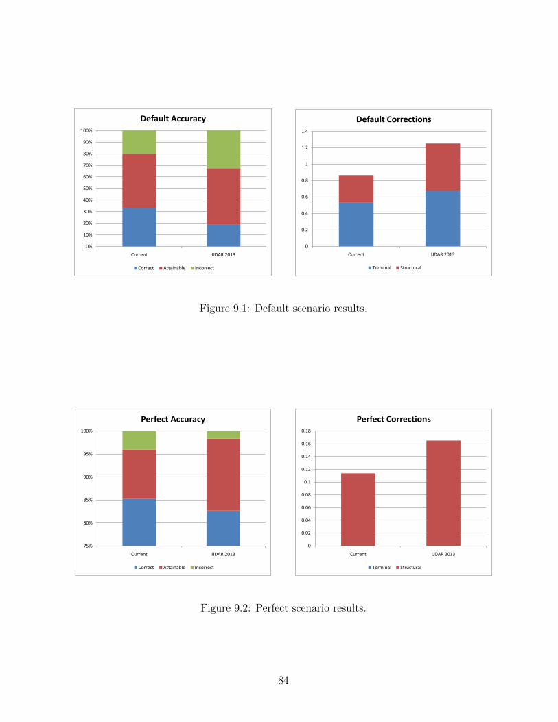
0%
10%
20%
30%
40%
50%
60%
70%
80%
90%
100%
Current IJDAR 2013
Default Accuracy
Correct Attainable Incorrect
0
0.2
0.4
0.6
0.8
1
1.2
1.4
Current IJDAR 2013
Default Corrections
Terminal Structural
Figure 9.1: Default scenario results.
75%
80%
85%
90%
95%
100%
Current IJDAR 2013
Perfect Accuracy
Correct Attainable Incorrect
0
0.02
0.04
0.06
0.08
0.1
0.12
0.14
0.16
0.18
Current IJDAR 2013
Perfect Corrections
Terminal Structural
Figure 9.2: Perfect scenario results.
84

comparable rates of 98% attainable (just over 0.16 corrections on average) and 83% correct.The current version again achieved a somewhat higher correctness rate, but in this scenariohad a slightly lower attainability rate. Rather than this indicating a problem with theprobabilistic recognizer, it likely indicates that the hand-coded rules of the fuzzy relationclassifier were too highly tuned for the 2009 training data. The large changes in theaccuracy rates of the rule-based relation classifier between the 2009 and 2011 testing datain Section 5.4 support this point.
9.2 Evaluation on the CROHME corpora
Since 2011, the CROHME math recognition competition has invited researchers to submitrecognition systems for comparative accuracy evaluation. In previous work, we comparedthe accuracy of a previous version of the MathBrush recognizer against that of the 2011entrants [22]. We also participated in the 2012 competition, placing second behind acorporate entrant [26]. In this section we will evaluate the current MathBrush recognizerdescribed in this thesis against its previous version as well as the other CROHME entrants.
The 2011 CROHME data is divided into two parts, each of which includes training andtesting data. The first part includes a relatively small selection of mathematical notation,while the second includes a larger selection. For details, refer to the competition paper[25]. The 2012 data is similarly divided, but also includes a third part, which we omit fromthis evaluation as it included notations not used by MathBrush (namely notations fromboolean logic such as overbar negations, etc.)
For each part of this evaluation, we trained our symbol recognizer on the same basedata set as in the previous evaluation and augmented that training data with all of thesymbols appearing in the appropriate part of the CROHME training data. The relationand grouping systems were trained on the 2011 Waterloo corpus. We used the the gram-mars provided in the competition documentation by converting them into the file formatrecognized by our parser.
The accuracy of our recognizer was measured using a perl script provided by the compe-tition organizers. In this evaluation, only the top-ranked parse was considered. There arefour accuracy measurements. Stroke reco. indicates the percentage of input strokes whichwere correctly recognized and placed in the parse tree. Symbol seg. indicates the percent-age of symbols for which the correct strokes were properly grouped together. Symbol reco.indicates the percentage of symbol recognized correctly, out of those correctly grouped.Finally, expression reco. indicates the percentage of expressions for which the top-rankedparse tree was exactly correct (corresponding to a “correct” result in our classificationscheme for the previous evaluation).
In Tables 9.1 and 9.2, the first two rows show the test results for the current versionof MathBrush using the fuzzy and probabilistic scoring funtions. In the first (2011) table,the third row shows evaluation results the version of our recognizer used for CROHME2012, the fourth row shows results from a previous publication [22], and the remainder of
85

the table is reproduced from the CROHME 2011 report [25]. In the second (2012) table,all rows but the first two are reproduced from the CROHME 2012 report [26].
Part 1 of corpus
Recognizer Stroke reco. Symbol seg. Symbol reco. Expression reco.
MathBrush prob. 93.16 97.64 95.85 67.40MathBrush fuzzy 92.20 96.54 95.65 62.43MathBrush (2012) 88.13 96.10 92.18 57.46MathBrush (2011) 71.73 84.09 85.99 32.04Rochester Institute of Tech. 55.91 60.01 87.24 7.18Sabanci University 20.90 26.66 81.22 1.66University of Valencia 78.73 88.07 92.22 29.28Athena Research Center 48.26 67.75 86.30 0.00University of Nantes 78.57 87.56 91.67 40.88
Part 2 of corpus
Recognizer Stroke reco. Symbol seg. Symbol reco. Expression reco.
MathBrush prob. 91.64 97.08 95.53 55.75MathBrush fuzzy 88.85 94.99 95.08 48.28MathBrush (2012) 87.08 95.47 92.20 47.41MathBrush (2011) 66.82 80.26 86.11 20.11Rochester Institute of Tech. 51.58 56.50 91.29 2.59Sabanci University 19.36 24.42 84.45 1.15University of Valencia 78.38 87.82 92.56 19.83Athena Research Center 52.28 78.77 78.67 0.00University of Nantes 70.79 84.23 87.16 22.41
Table 9.1: Evaluation on CROHME 2011 corpus.
These results indicate that the MathBrush recognizer is significantly more accuratethan all other entrants except the Vision Objects recognizer, which is much more accurateagain. (Vision Objects is a French company based in Nantes). They are of more interest forour purpose because they allow us to roughly compare different versions of the MathBrushrecognizer on a subsystem-by-subsystem basis. The comparison can only be approximatebecause correctness is evaluated based on the single top-ranked interpretation of the input,which depends on a complex combination of the individual subsystems.
The accuracy of the stroke grouping system is roughly equivalent to the 2012 versionof MathBrush. This is expected as the algorithms used are very similar. The symbolrecognizer in the 2012 was a preliminary version of the hybrid recognizer described herewith a simpler version of the offline classifier; the changes have led to a modest improvementin accuracy (roughly 3% in absolute terms, but a 40-50% reduction in errors). It is difficultto determine exactly how much of the improvement in the expression recognition rateis due to symbol recognition as compared with the probabilistic relation classifier or theoverall probabilistic scoring function, both of which were not present in the 2012 recognizer,which used the rule-based relation classifier and the fuzzy scoring function. But given themagnitude of some of the improvements, especially in Part 1 of these corpora, it seemsunlikely that all of the improvement was due to increased symbol recognition accuracy.
86

Part 1 of corpus
Recognizer Stroke reco. Symbol seg. Symbol reco. Expression reco.
MathBrush prob. 91.54 96.56 94.83 66.36MathBrush fuzzy 90.72 95.56 93.96 56.07MathBrush (2012) 89.00 97.39 91.72 51.85University of Valencia 80.74 90.74 89.20 35.19Athena Research Center 59.14 73.31 79.79 8.33University of Nantes 90.05 94.44 95.96 57.41Rochester Institute of Tech. 78.24 92.81 86.62 28.70Sabanci University 61.33 72.11 87.76 22.22Vision Objects 97.01 99.24 97.80 81.48
Part 2 of corpus
Recognizer Stroke reco. Symbol seg. Symbol reco. Expression reco.
MathBrush prob. 92.74 95.57 97.05 55.18MathBrush fuzzy 89.82 94.49 95.73 42.47MathBrush (2012) 90.71 96.67 94.57 49.17University of Valencia 85.05 90.66 91.75 33.89Athena Research Center 58.53 72.19 86.95 6.64University of Nantes 82.28 88.51 94.43 38.87Rochester Institute of Tech. 76.07 89.29 91.21 14.29Sabanci University 49.06 61.09 88.36 7.97Vision Objects 96.85 98.71 98.06 75.08
Table 9.2: Evaluation on CROHME 2012 corpus.
87

Chapter 10
Conclusion
This thesis described the theory and implementation details underlying the MathBrushmath recognizer. Building from low-level distance metrics and classification routines, wedetailed the components and combination strategies underlying our sophisticated and ac-curate recognition system. This chapter summarizes the thesis, pointing out primarycontributions and offering thoughts on future research directions.
10.1 MathBrush requirements
Chapter 1 listed the three requirements placed upon the recognizer by the MathBrushsystem in which it is used:
• it must be reasonably fast,
• it must be trainable, and
• it must support user corrections.
We made significant efforts to ensure that the recognizer is fast enough for real-time use,including the linear-time variant of elastic matching (Section 4.1.2), the ordering assump-tion and corresponding restriction to rectangular sets (Section 7.2.1), and the optimizationsapplied to Unger’s algorithm (Section 7.2.2). In practice, the recognizer is quick enoughto use comfortably on the Tablet PC platform for most inputs. However, on less powerfultablet devices (such as Android tablets and the iPad) and for large expressions, there isoften a delay after adding a stroke to the input. User studies would help to determinethe impact of such delays on the input process. If they are a significant impediment toeffective use of MathBrush, it would be worthwhile to investigate additional optimizations,including:
• Judicious use of pruning to avoid invoking the parser on input subsets or non-terminals which are unlikely to yield useful results.
88
• A fast pre-processing step which could avoid invoking the full parsing algorithm byfirst considering a small number of likely parses incorporating a new input stroke.
• Using a single symbol recognition algorithm (rather than four), and only invoking thehybrid classifier in case of ambiguity. This could be driven by data collected aboutrecognizer behaviour.
To facilitate user training, our symbol recognizer easily accomodates new symbol stylesby adding them to the symbol library, as described in Section 4.1. This process is madefairly simple by the MathBrush interface, which prompts the user to write the symbol theywish to train in a few on-screen ink collection areas. The training process for the relationclassifier is much less straightforward and is not exposed to users. However, the correctionswhich users make to change erroneous recognition results are a rich and currently un-tappedsource of training information. Future research should investigate how those correctionscan be used to create custom-trained writer-dependent recognizers, as well as how thosecorrections may be pooled to improve the writer-independent baseline recognizer.
The correction process itself is made possible by our use of parse forests (Section 7.1),the tree extraction algorithms described in Section 7.3, and the scoring models of Chapter8. Because the parse forest generally represents exponentially many trees in the inputsize, the “semantics mode” of tree extraction is vital for keeping the number of displayedresults manageable for users. All the same, the correction count employed in Section 9.1as a user-centric accuracy metric was measured automatically, rather than by observingreal users. User studies would indicate to what extent our correction system is truly animprovement over erasing and re-writing when input is mis-recognized.
10.2 Low-level classifiers
Chapters 3, 4, and 5 respectively discussed our approaches to stroke grouping, symbolrecognition, and relation classification. We developed a novel stroke-grouping system basedon translating logic- and rule-based heuristics into the language of binary random variables.This system reported false negatives only about 0.5% of the time, was correct by thestrictest definition about 90% of the time, and obtained the correct grouping result in apractical context in about 96% of cases.
We proposed a hybrid symbol classification method using four underlying distance-based classifiers, including a novel time- and space-optimized variant of the well-knownelastic matching algorithm. The hybrid method attained a correctness rate of about 88%on isolated symbols, an improvement on the correctness rates of the underlying classifiers,which ranged from about 75-85%. During testing on the CROHME data set, the recognizerreached even higher correctness rates of 95-97%; however these results were on a smallerset of symbols than is present in the Waterloo corpus.
The correctness rates of both of these systems must be improved in order to improveoverall recognition quality. As well as developing new recognition algorithms or adapt-ing existing methods to a mathematical context, improvement may be possible through
89

combining the grouping and recognition modules more closely. Whether a collection ofstrokes should be considered a symbol certainly depends on whether those strokes actuallylook like a known symbol, yet that information is not taken into account in our system(except in the case of square root signs to determine whether stroke overlap is acceptableor not). The main challenge in combining the two systems is to maintain real-time per-formance. Symbol recognition is an expensive step, and applying it to every stroke subsetthe grouping system considers is not practical.
Several techniques were proposed and evaluated for relation classification, including arule-based heuristic approach and three probabilistic techniques: a naive Bayesian modelusing Gaussian distributions, a grid-based discretization strategy, and a second discretiza-tion method using the margin tree data structure which we developed. Both the discretiza-tion techniques performed very well in isolated testing with correctness rates of about 95%.But in the full context of math recognition, they proved less able to distinguish betweencases where a relation existed and did not exist, so we use the naive Bayesian approach inpractice. The majority of relation classification errors occur on the horizontally-orientedrelations ↗ ,→ , and ↘ because of the natural ambiguity of bounding box features. Im-provements using the same feature set should rely on more context-sensitive models (whichin turn require more training data). Given the effectiveness of the quantile-based methodused for combining symbol classifiers, it seems worthwhile to apply that technique to the re-lation classifiers as well. Also, the present classifers use only information local to the strokegroups in question. Considering how the expressions resulting from each candidate relationwould fit into the larger picture may also yield improvements. During our experiments withfuzzy sets, estimating global baselines and measuring how well a given relation matched itsexpected placement with respect to the baseline yielded modest improvements in relationclassification accuracy. Finally, the hybrid symbol recognizer described in Chapter 4 wasmore accurate than any of the underlying individual recognizers. A similar quantile-basedcombination method may improve accuracy for the relation classification task as well.
10.3 Grammars and parsing
Chapter 6 developed a novel relational grammar formalism offering sophisticated controlover subexpression combination through linkage parameters. The linkage parameters arequite powerful, and we observed a significant increase in recognition accuracy after in-corporating them into our grammar model. We adapted familiar notions such as stringsand languages to our model, and described how the grammar formalism relates to therecognition process. Chapter 7 built efficient parsing algorithms for this grammar model,inspired by classic CFG parsing algorithms. By introducing some natural assumptionson the structure of the input and scoring algorithms, we attained acceptable performancefor real-time use. The algorithms maintain a user-centric design by making available allrecognizable interpretations of the input and organizing those results hierarchically so thatthe user may select alternative recognition results rather than re-writing their expressionif recognition is incorrect.
The ordering assumption is reasonable in theory, but is sometimes violated in practice,
90

even on expressions that are easily readable by people. It would be beneficial to eliminateor weaken the assumption as much as possible while still achieving fast recognition speedand avoiding consistent worst-case behaviour as in the CYK parsing algorithm. A well-specified and efficient method of identifying all “reasonable” combinations of rectangularsets which cover the input would improve accuracy without unduly affecting performance.
10.4 Scoring methods
Finally, Chapter 8 detailed two scoring functions on which to base the rank-based reportedscheme of Chapter 7. The fuzzy scoring function simply treats the sets of interpretationsintroduced in Chapter 6 as fuzzy sets and define a membership function on them using thegeometric average. The probabilistic scoring function treats the expressions and symbolsrecognized on input subsets as random variables and organizes them in a Bayesian model.An algebraic technique dramatically reduces the number of variables it is necessary toconsult when evaluating the score of a given parse tree.
In our evaluation, the probabilistic model was more effective than the fuzzy model.This is not surprising, given its greater sophistication and inclusion of more details (e.g.,symbol co-occurrence counts, nil probabilities, etc.). The relative ease with which suchdetails can be systematically included in an expression’s score is a real strength of theprobabilistic approach, and the addition of more real-world data would likely further im-prove performance. We have developed a preliminary implementation that assigns a priordistribution to the expression variables based on known subexpression occurrences and soon. (E.g., addition expressions are more likely to contain subscripts than function names,etc.) But we currently lack sufficient data for such a model to be useful. The number ofpotential subexpression combinations is very large, and the resulting look-up tables are sosparsely populated that they give nonsense answers to queries even when using smoothing.Nonetheless, this remains a promising idea for the future, when larger collections of mathexpressions may be available.
91

References
[1] Francisco Alvaro, Joan-Andreu Sanchez, and Jose-Miguel Benedı. Recognition ofprinted mathematical expressions using two-dimensional stochastic context-free gram-mars. In Proc. of the Int’l. Conf. on Document Analysis and Recognition, pages 1225–1229, 2011.
[2] Robert H. Anderson. Syntax-Directed Recognition of Hand-Printed Two-DimensionalMathematics. PhD thesis, Harvard University, 1968.
[3] A.-M. Awal, H. Mouchere, and C. Viard-Gaudin. The problem of handwritten math-ematical expression recognition evaluation. In Proc. of the Int’l. Conf. on Frontiersin Handwriting Recognition, pages 646–651, 2010.
[4] Dorothea Blostein. Math-literate computers. In Jacques Carette, Lucas Dixon, Clau-dio Sacerdoti Coen, and Stephen M. Watt, editors, Calculemus/MKM, volume 5625of Lecture Notes in Computer Science, pages 2–13. Springer, 2009.
[5] Kam-Fai Chan and Dit-Yan Yeung. Error detection, error correction and performanceevaluation in on-line mathematical expression recognition. In in On-Line Mathemat-ical Expression Recognition,” Pattern Recognition, 1999.
[6] Kam-Fai Chan and Dit-Yan Yeung. Error detection, error correction and perfor-mance evaluation in on-line mathematical expression recognition. Pattern Recognition,34(8):1671 – 1684, 2001.
[7] U. Garain and B.B. Chaudhuri. Recognition of online handwritten mathematicalexpressions. Systems, Man, and Cybernetics, Part B: Cybernetics, IEEE Transactionson, 34(6):2366–2376, Dec. 2004.
[8] Utpal Garain and B. Chaudhuri. A corpus for ocr research on mathematical expres-sions. Int. J. Doc. Anal. Recognit., 7(4):241–259, 2005.
[9] Oleg Golubitsky and Stephen M. Watt. Online computation of similarity betweenhandwritten characters. In Proc. Document Recognition and Retrieval XVI, 2009.
[10] Dick Grune and Ceriel J.H. Jacobs. Parsing Techniques: A Practical Guide. Springer,2 edition, 2008.
92

[11] David Hoaglin, Frederick Mostaller, and John Tukey (editors). Understanding Robustand Exploratory Data Analysis. John Wiley & Sons, 1983.
[12] Jesse Hull. Recognition of mathematics using a two-dimensional trainable context-freegrammar. Master’s thesis, Massachusetts Institute of Technology, 1996.
[13] G. Labahn, E. Lank, S. MacLean, M. Marzouk, and D. Tausky. MathBrush: A systemfor doing math on pen-based devices. The Eighth IAPR Workshop on DocumentAnalysis Systems (DAS), pages 599–606, 2008.
[14] G. Labahn, E. Lank, M. Marzouk, A. Bunt, S. MacLean, and D. Tausky. MathBrush:A case study for interactive pen-based mathematics. Fifth Eurographics Workshop onSketch-Based Interfaces and Modeling (SBIM), June 11-13 2008.
[15] Bernard Lang. Towards a uniform formal framework for parsing. In Current Issuesin Parsing Technology, pages 153–171. Kluwer Academic Publishers, 1991.
[16] Joseph J. Laviola, Jr. Mathematical sketching: a new approach to creating and ex-ploring dynamic illustrations. PhD thesis, Brown University, 2005.
[17] Joseph J. LaViola, Jr. and Robert C. Zeleznik. Mathpad2: a system for the creationand exploration of mathematical sketches. In SIGGRAPH ’04: ACM SIGGRAPH2004 Papers, pages 432–440, New York, NY, USA, 2004. ACM.
[18] Percy Liang, Mukund Narasimhan, Michael Shilman, and Paul Viola. Efficient ge-ometric algorithms for parsing in two dimensions. In ICDAR ’05: Proceedings ofthe Eighth International Conference on Document Analysis and Recognition, pages1172–1177, Washington, DC, USA, 2005. IEEE Computer Society.
[19] W. Liu, L. Zhang, L. Tang, and D. Dori. Cost evaluation of interactively correctingrecognized engineering drawings. Lecture Notes in Computer Science, 1941:329–334,2000.
[20] S. MacLean, G. Labahn, E. Lank, M. Marzouk, and D. Tausky. Grammar-basedtechniques for creating ground-truthed sketch corpora. Int’l. J. Document Analysisand Recognition, 14:65–74, 2011.
[21] S. MacLean, D. Tausky, G. Labahn, E. Lank, and M. Marzouk. Is the iPad usefulfor sketch input?: a comparison with the Tablet PC. In Proceedings of the EighthEurographics Symposium on Sketch-Based Interfaces and Modeling, SBIM ’11, pages7–14, 2011.
[22] Scott MacLean and George Labahn. A new approach for recognizing handwrittenmathematics using relational grammars and fuzzy sets. International Journal on Doc-ument Analysis and Recognition (IJDAR), 16(2):139–163, 2013.
[23] Christopher D. Manning and Hinrich Schuetze. Foundations of Statistical NaturalLanguage Processing. The MIT Press, 1999.
93

[24] Erik G. Miller and Paul A. Viola. Ambiguity and constraint in mathematical expres-sion recognition. In Proceedings of the fifteenth national/tenth conference on Artificialintelligence/Innovative applications of artificial intelligence, pages 784–791, 1998.
[25] H. Mouchere, C. Viard-Gaudin, U. Garain, D.H. Kim, and J.H. Kim. CROHME2011:Competition on recognition of online handwritten mathematical expressions. In Proc.of the 11th Int’l. Conference on Document Analysis and Recognition, 2011.
[26] H. Mouchere, C. Viard-Gaudin, U. Garain, D.H. Kim, and J.H. Kim. Competitionon recognition of online handwritten mathematical expressions (CROHME 2012). InProc. of the 11th Int’l. Conference on Frontiers in Handwriting Recognition, 2012.
[27] I. Rutherford. Structural analysis for pen-based math input systems. Master’s thesis,David R. Cheriton School of Computer Science, University of Waterloo, 2005.
[28] K. Sain, A. Dasgupta, and U. Garain. Emers: a tree matching-based performanceevaluation of mathematical expression recognition systems. IJDAR, 14(1):75–85, 2011.
[29] Yu Shi, HaiYang Li, and F.K. Soong. A unified framework for symbol segmentationand recognition of handwritten mathematical expressions. In Document Analysis andRecognition, Ninth International Conference on, pages 854–858, 2007.
[30] Masakazu Suzuki, Seiichi Uchida, and Akihiro Nomura. A ground-truthed mathe-matical character and symbol image database. Document Analysis and Recognition,International Conference on, pages 675–679, 2005.
[31] Charles C. Tappert. Cursive script recognition by elastic matching. IBM Journal ofResearch and Development, 26(6):765–771, 1982.
[32] Arit Thammano and Sukhumal Rugkunchon. A neural network model for onlinehandwritten mathematical symbol recognition. Lecture Notes in Computer Science,4113, 2006.
[33] Stephen H. Unger. A global parser for context-free phrase structure grammars. Com-mun. ACM, 11:240–247, April 1968.
[34] Merijn van Erp and Lambert Schomaker. Variants of the borda count method for com-bining ranked classifier hypotheses. In L.R.B. Schomaker and L.G. Vuurpijl, editors,Proceedings of the Seventh Int’l. Workshop on Frontiers in Handwriting Recognition,pages 443–452, 2000.
[35] H.-J. Winkler, H. Fahrner, and M. Lang. A soft-decision approach for structuralanalysis of handwritten mathematical expressions. In Proc. International Conferenceon Acoustics, Speech and Signal Processing, pages 2459–2462, 1995.
[36] R. Yamamoto, S. Sako, T. Nishimoto, and S. Sagayama. On-line recognition of hand-written mathematical expression based on stroke-based stochastic context-free gram-mar. In The Tenth International Workshop on Frontiers in Handwriting Recognition,2006.
94

[37] L.A. Zadeh. Fuzzy sets. Information Control, 8:338–353, 1965.
[38] R. Zanibbi, D. Blostein, and J.R. Cordy. Baseline structure analysis of handwrittenmathematics notation. In Document Analysis and Recognition, 2001. Proceedings.Sixth International Conference on, pages 768–773, 2001.
[39] R. Zanibbi, D. Blostein, and J.R. Cordy. Recognizing mathematical expressions usingtree transformation. Pattern Analysis and Machine Intelligence, IEEE Transactionson, 24(11):1455–1467, Nov 2002.
[40] Robert Zeleznik, Timothy Miller, Chuanjun Li, and Joseph J. Laviola, Jr. Mathpa-per: Mathematical sketching with fluid support for interactive computation. In SG’08: Proceedings of the 9th international symposium on Smart Graphics, pages 20–32,Berlin, Heidelberg, 2008. Springer-Verlag.
[41] Ling Zhang, D. Blostein, and R. Zanibbi. Using fuzzy logic to analyze superscript andsubscript relations in handwritten mathematical expressions. In Document Analysisand Recognition, 2005. Proceedings. Eighth International Conference on, pages 972–976 Vol. 2, 2005.
95