automated terrestrial laser scanning with near-real … terrestrial laser scanning with near ... and...

Earth Surf. Dynam., 5, 293–310, 2017www.earth-surf-dynam.net/5/293/2017/doi:10.5194/esurf-5-293-2017© Author(s) 2017. CC Attribution 3.0 License.

Automated terrestrial laser scanning with near-real-timechange detection – monitoring of the Séchilienne

landslide

Ryan A. Kromer1,2, Antonio Abellán1,2,3, D. Jean Hutchinson2, Matt Lato2,5, Marie-Aurelie Chanut4,Laurent Dubois4, and Michel Jaboyedoff1

1Risk Analysis Group, University of Lausanne, Lausanne, Switzerland2Geomechanics Group, Geological Sciences and Geological Engineering, Queen’s University,

Kingston, Ontario, Canada3Scott Polar Research Institute, University of Cambridge, Cambridge, UK

4Groupe Risque Rocheux et Mouvements de Sols (RRMS), Cerema Centre-Est, France5BGC Engineering, Ottawa, Canada

Correspondence to: Ryan A. Kromer ([email protected])

Received: 23 January 2017 – Discussion started: 30 January 2017Revised: 11 April 2017 – Accepted: 20 April 2017 – Published: 24 May 2017

Abstract. We present an automated terrestrial laser scanning (ATLS) system with automatic near-real-timechange detection processing. The ATLS system was tested on the Séchilienne landslide in France for a 6-weekperiod with data collected at 30 min intervals. The purpose of developing the system was to fill the gap ofhigh-temporal-resolution TLS monitoring studies of earth surface processes and to offer a cost-effective, light,portable alternative to ground-based interferometric synthetic aperture radar (GB-InSAR) deformation monitor-ing. During the study, we detected the flux of talus, displacement of the landslide and pre-failure deformation ofdiscrete rockfall events. Additionally, we found the ATLS system to be an effective tool in monitoring landslideand rockfall processes despite missing points due to poor atmospheric conditions or rainfall. Furthermore, such asystem has the potential to help us better understand a wide variety of slope processes at high levels of temporaldetail.

1 Introduction

terrestrial laser scanning (TLS) is extensively used in theearth sciences to understand and monitor earth surface prop-erties and processes (Eitel et al., 2016). It is commonly usedto create dense three-dimensional (3-D) point clouds or dig-ital elevation models to map and characterize the earth sur-face, and to better understand surface processes by compar-ing multiple acquisitions over time. Dense 3-D data are alsoused to quantify and characterize natural hazards (Jaboyed-off et al., 2012) and to monitor hazard processes (Barbarella,2013; Rosser et al., 2005; Royán et al., 2013; Travelletti etal., 2008). The use of TLS and other remote sensing tech-nologies now forms an important part of natural hazard risk

management approaches (Corominas et al., 2014; Jaboyedoffet al., 2012; Metternicht et al., 2005).

Many studies have used multitemporal TLS (> month, de-fined by Eitel et al., 2016) to monitor landslide processes(Abellán et al., 2010; Avian et al., 2009; Bremer and Sass,2012; Dewitte et al., 2008; Lague et al., 2013; Lato et al.,2014; Lim et al., 2005; Oppikofer et al., 2008; Rosser et al.,2005; Royán et al., 2015; Schürch et al., 2011; Teza et al.,2007; Travelletti et al., 2008); the use of TLS at a hyper-temporal level (< month, defined by Eitel et al., 2016), how-ever, is limited (e.g. Kromer et al., 2015a, b; Milan et al.,2007; Oppikofer et al., 2008). Additionally, monitoring at> daily intervals, here defined as super-temporal monitoring,still represents a challenge and has yet to be exploited, espe-cially over long-duration temporal monitoring periods. Fully

Published by Copernicus Publications on behalf of the European Geosciences Union.

294 R. A. Kromer et al.: Automated terrestrial laser scanning

utilizing the spatial (x,y,z) and time dimensions in earth sur-face process studies represents one of the major growth areasof TLS research, as pointed out by the review paper by Eitelet al. (2016).

Studying earth processes at a super-temporal level withTLS has many possible advantages. It would reduce or elim-inate the problem of event superposition and coalescencewhen monitoring geomorphic events too infrequently, as dis-cussed in Lim et al. (2005). With frequent scanning mea-surement, uncertainties can be significantly reduced by tak-ing advantage of the large number of spatial and temporalmeasurements collected (Abellán et al., 2009, 2013; Kromeret al., 2015b). Furthermore, in landslide emergencies, a TLSsystem would be highly beneficial as it can be easily trans-ported, set up rapidly, and can be carried through ruggedand remote areas. A TLS-based warning system would bea light, portable, cost-effective alternative to ground-basedinterferometric synthetic aperture radar (GB-InSAR) moni-toring technologies.

The key challenges in using TLS to study earth pro-cesses at the super-temporal level is the high cost of frequentdata acquisitions and challenges in processing and manag-ing large numbers of data (Orem and Pelletier, 2015). Theadvent of automated terrestrial laser scanners (ATLSs) hasmade high-temporal-resolution terrestrial acquisitions eas-ier (Adams et al., 2013; Eitel et al., 2013); however, auto-matic processing of the data is still required to relieve thepost-processing burden. This is especially important for land-slide early warning monitoring, where processed results areneeded as soon as possible for decision makers.

The aim of this paper is to detail the development of anATLS system with automatic near-real-time data processingand its application at a test landslide site. We demonstratethe feasibility and limitations of a near-real-time monitoringsystem and demonstrate how the system can be used to mon-itor pre-failure deformation of landslides and discrete rock-fall events. The system may be suitable for a wide range ofapplications in the earth sciences, including monitoring ofsoil erosion, volcanic activity, fault movement and glacierdynamics, for example.

2 Study site description

We conducted our experiment at the Séchilienne landslide,located 20 km southeast of Grenoble in France along RD1091 Grenoble–Briancon in the Romanche Valley of theFrench Alps (Fig. 1). This landslide was chosen for the exper-iment because its geological characteristics, movement, hy-drology and hydrochemistry have been well studied (Baude-ment et al., 2013; Chanut et al., 2013; Dubois et al., 2014;Dunner et al., 2011; Guglielmi et al., 2002; Helmstetter andGarambois, 2010; Kasperski et al., 2010; Le Roux et al.,2011); existing infrastructure at the site made it ideal for test-ing the TLS system (Duranthon, 2006); and the variety of ac-

tive slope processes, including displacement of the landslide,frequent rockfalls and movement of talus or scree material.

Kasperski et al. (2010) describe two parts of the landslide,an active frontal zone, known as “Les Ruines”, and subsi-dence of the upper part of the Mont-Sec slope between 600and 1180 m above sea level (a.s.l.) comprising an area of70 ha, outlined in Fig. 1. The upper Mont-Sec slope is de-limited by a 20 to 40 m high scarp (Helmstetter and Garam-bois, 2010). Over the past century the “Les Ruines” area hasbeen a source of frequent rockfalls (Le Roux et al., 2011).Early studies of the landslide revealed the risk of collapseof 2 to 3 million m3 from the frontal zone and the instabil-ity encompassing Mont-Sec at around 20 to 30 million m3

(Evrard et al., 1990). More recent estimates of the landslidedepth using geophysics put the frontal zone at 3 million m3

and the Mont-Sec instability at 60 million m3 (Le Roux etal., 2011). However, these volumes were established with-out precise knowledge of the slope deformation mechanismand are undoubtedly under-evaluated given the field data ac-quired since.

Geologically, the landslide is part of the external crys-talline massif of Belledonne. The landslide mainly con-sists of mica schists, which are composed of alternatingmetamorphic sandstones and siltstones. Pothérat and Al-fonsi (2001) identified several faults intersecting the land-slide and three sets of near-vertical fractures: N20◦, N120◦

and N70◦. Detailed description of the geology of the land-slide and surrounding area can be found in Helmstetter andGarambois (2010), Kasperski et al. (2010) and Le Roux etal. (2011).

The French public national body, Cerema, has been mon-itoring the landslide since 1985 (Dubois et al., 2014; Duran-thon, 2006). Multiple monitoring techniques are used on thelandslide including 31 extensometers, 30 radar targets, 65 in-frared targets, and 2 boreholes with slope inclinometers andGPS receivers. A total station, a radar unit and a permanentcamera station are located on the opposite side of the valleyinside the Mont Falcon Station (shown in Fig. 3). Movementat depth is monitored using a 240 m long exploration aditand three 150 m depth boreholes in the high-motion zones.A seismic monitoring system has been in place since 2008.The system consists of three seismological stations and re-ceivers that record rockfall events and local- and regional-scale earthquakes (Helmstetter and Garambois, 2010).

Displacement of the landslide ranges from 0.01 to 0.10 mper year except at the level of the frontal zone in the eastwhere displacements reach up to 3.5 m per year (Dubois etal., 2014). Figure 2 plots the displacement of extensome-ter A13 located in this frontal zone since 1994. Dubois etal. (2014) divided the landslide evolution into three main dis-placement phases:

– From 1994 to 2006, seasonal fluctuations of the dis-placement rates were observed in connection with pre-cipitation (rain and snowmelt).

Earth Surf. Dynam., 5, 293–310, 2017 www.earth-surf-dynam.net/5/293/2017/

R. A. Kromer et al.: Automated terrestrial laser scanning 295

Figure 1. (a) Location of the Séchilienne rock slope in the Romanche River valley along RD 1091. The landslide is outlined in whitecovering an area known as the Mont-Sec slope. The most active frontal zone is outlined in yellow. (b) Digital terrain model (DTM) of theMont-Sec slope with most active frontal zone of the landslide highlighted. (c) Location of the Séchilienne landslide within France.

Raw velocity Annual mean velocity

Seasonal fluctua�ons Increasing displacements

Decreasing Displacements

Jan 2006 Jan 2013

Jan 1994 Jan 1999 Jan 2004 Jan 2009 Jan 2014

A13

velo

city

(mm

day

–1)

20

18

16

14

12

10

8

6

4

2

0

Figure 2. Velocity in mm day−1 at extensometer A13 from 1 Jan-uary 1994 until 31 March 2015 (black), and annual mean velocity(blue; Dubois et al., 2014).

– From 2006 to December 2012, there were less fluctua-tions of the displacement rates and a general increase ofthe average velocity.

– Since January 2013, a decrease in average velocity hasbeen observed. This decrease has been strong since July2013, then stronger since spring 2014. It has reached−85 % of peak velocity between end of June 2013 andend of July 2015.

Vallet et al. (2015) found that groundwater fluctuations ex-plain the periodic variations in displacement and the long-term exponential trend, interpreted as a consequence of

weakening of rock due to groundwater pressure action. Thelandslide shows signs of deep-seated gravitational deforma-tion with displacement revealing a complex structure withcone sheet fractures, counterscarps, and depletion and ac-cumulation zones. Kasperski et al. (2010) interpret a land-slide failure mechanism of toppling and subsidence of ver-tical rock layers. Frequent measurements since 2009 sup-port this interpretation revealing a deformation mechanismof deep flexural toppling without a basal failure plane.

In addition to the monitoring network, multi-temporalTLS (seven acquisitions between 2004 and 2009; Kasper-ski, 2008; and an additional five TLS scans from 2009 to2015; Vulliez, 2016), multi-temporal aerial laser scanning(2011 and 2014) and terrestrial photogrammetry (2015) wereconducted at the site (Vulliez, 2016). The goal of these datacollections was to provide continuous spatial coverage of thelandslide movement with a focus on the active frontal zone.The studies have helped characterize the instability and dis-placement patterns and have helped better elucidate the fail-ure mechanism; however, prior to this study, high-spatial-density hyper- and super-temporal data have not been ac-quired.

3 Methods

We designed the hardware components of the monitoringsystem described in Sect. 3.1 for the study of landslide,talus and rockfall processes at the Séchilienne landslide site.The hardware components were designed for a temporary(months) installation and took advantage of existing infras-

www.earth-surf-dynam.net/5/293/2017/ Earth Surf. Dynam., 5, 293–310, 2017


Figure 3. Setup of the ATLS monitoring system at the Ceremamonitoring centre in Séchilienne, France, which consisted of (a) theTLS system and protective housing installed on the roof the centre;(b) a notebook installed inside the monitoring centre for near-real-time data processing and data visualization; and (c) TLS, tilting baseand battery backup built within a protective housing.

tructure available at the study site, a concrete monitoringcentre operated and maintained by Cerema. The hardwarecould be adapted for other use cases, for example a tempo-rary monitoring installation in the order of days could beoperated using a tripod and a generator, whereas a longer-term installation could be installed with a permanent pro-tective housing, solar panels and batteries. The processingworkflow described in Sect. 3.2 was designed to monitorearth surface processes in near-real time, defined as imme-diate post-processing after collection, taking less time thanthe time between scans. In this section, we point out designelements that are specific to the study of landslides and theTLS scanner used. For example, for the study of pre-failuredeformation of rockfalls or landslide displacements, the tim-ing of processing is critical to be able to provide timely warn-ing of a potential imminent failure event and the workflow isdesigned to process data as quickly as possible after data col-lection. Specific input parameters pertinent to our study caseand to landslide processes are described in Sect. 3.3.

3.1 Site setup and hardware components

We used an Optech ILRIS long-range (LR) laser scanner(Teledyne Optech, 2014a) for this study. We installed theTLS system on the roof of the monitoring centre (Fig. 3a). Toprotect the TLS system against the elements, we constructeda wooden encasement painted with a weather-resistant coat-ing (Fig. 3c). The encasement housed the TLS, the batterybackup, a manual tilt, power and Ethernet cables. We de-signed the front opening of the encasement so that it allowed±10◦ of tilt but was still small enough to not allow the TLSto be removed. We opted for an open design compared to

TLS data acquisi�on

4-D filter algorithm

Registra�on pipeline

Pretreatment and point cloud rejec�on

Visualiza�on Re

peat

for e

ach

poin

t clo

ud

Figure 4. Near-real-time data processing workflow consisting of adata automated acquisition module, a pre-treatment and point cloudrejection stage, a rejection pipeline consisting of an initial align-ment and an iterative fine alignment stage, a 4-D filtering and dis-tance calculation algorithm (Kromer et al., 2015b) and a visualiza-tion module. This workflow is repeated for each point cloud acqui-sition.

one with an infrared permeable screen to maximize the inter-cepted returns and to allow natural ventilation of the equip-ment. Earlier testing through various glass mediums revealedinterference with the signal return. To further increase ven-tilation, we included slits in both the side and back panelsof the encasement. A lid covered the top of the encasementand extended in front of the viewing opening to minimizethe amount of water entering the encasement. We bolted theencasement to the top of the monitoring centre structure andused chain and locks for theft protection. The TLS systemwas supplied with power via cables connected to the interiorof the monitoring centre.

Data from the TLS system were transferred from the sys-tem to an on-site computer located in the interior of the mon-itoring centre (Fig. 3b). The purpose of the computer was forautomated near-real-time data processing and visualizationof the results. Data were stored on both the computer harddrive and on external backup drives. The computer consistedof an ordinary notebook (HP Elitebook 8740w) with a dual-



Ini�al alignment

Normal calcula�on at each point

Repe

at u

n�l t

erm

ina�

on cr

iterio

n m

et

Es�mate rigid transforma�on

Feature defini�on at keypoints using fast

point feature histogram

Keypoint selec�on using intrinsic shape

signatures

Search for correspondences between features

Correspondence rejec�on using

RANSAC

Es�mate rigid transforma�on

Search for correspondences

Correspondence rejec�on using

RANSAC, normal and median

Ini�al alignment Fine alignment

Figure 5. Registration pipeline workflow consisting of an initialalignment stage and a fine alignment stage. The initial alignmentstage aligns two point clouds independent of orientation and po-sition and is based on keypoint and descriptor matching. The finealignment stage is an iterative corresponding point variant consist-ing of a matching, rejection and alignment stage.

core 2.67 GHz Intel Core i7 processor and 4.0 GB of RAM.The computer was connected to the internet via a cellularlink. This allowed the entire system to be operated and thedata visualized remotely via remote control software.

3.2 Processing workflow design

Processing point clouds for change detection analysis typi-cally involves several manual steps. These steps involve man-ually removing vegetation and erroneous points, picking sim-ilar points between successive point clouds for an initial es-timation of the registration transformation matrix, an appli-cation of the iterative closest point (ICP) algorithm for align-ment, the building of a meshed surface model and the cal-culation of distances (methods reviewed in Abellán et al.,2014). This manual process cannot be performed for scan-ners operating almost continuously and automation of thesesteps is required. Furthermore, the processing must happenrapidly so that the results can be interpreted in sufficient timein emergency scenarios, i.e. an impending landslide.

We designed the processing workflow of the system to op-erate the scanner at set intervals and to process the data innear-real time. The processing workflow consists of modules

to operate the scanner automatically, to manage and backup data, and to automatically process the data. Due to in-tellectual property restrictions, we could not design our ownmodule to operate the scanner; instead, we used Optech’s IL-RIS Command Line (ICL) application version 1.6.7 (Tele-dyne Optech, 2014b), which initiates a scan with predefinedscan parameters. We designed a data processing module tointercept the incoming scan data from the ICL application.The data processing module was developed using C++ withQT and the Point Cloud Library (PCL; Rusu and Cousins,2011) and is outlined in Fig. 4. The first phase of the pro-cessing module consists of pre-processing steps: (a) removalof unwanted points using a pass-through filter and (b) a qual-ity control (QC) step consisting of the rejection of a pointcloud if it does not contain a specified minimum number ofpoints, which is commonly due to poor atmospheric condi-tions or rainfall. This stage also applies an atmospheric cor-rection to the point clouds. The second step is registration ofthe point cloud to a reference through a registration pipelineconsisting of an initial alignment stage followed by an iter-ative fine alignment stage. The initial alignment stage wasdesigned to align the point clouds if the scan position hasbeen changed, but in general it is used as a good initial start-ing point to speed up the iterative registration process. Theinitial alignment consists of finding repeatable keypoints inthe point cloud, defining descriptors based on the local key-point point neighbourhoods and finding correspondences be-tween features to perform an initial transformation. Refinedalignment is conducted by iteratively transforming the pointcloud, finding correspondences and using a rejector pipelineto discard poor correspondences until a convergence crite-rion is met (Fig. 5). Change detection is conducted by cal-culating slope-dependent change vectors and filtering noiseusing neighbours in space and time (Kromer et al., 2015b).The processed points clouds are visualized in near-real timeusing a visualizer designed using a PCL visualizing module,and change time series data are plotted using Matlab (TheMathworks Inc.). A detailed description of this workflow fol-lows in Sect. 3.2.1 through 3.2.5.

3.2.1 TLS data acquisition

ILRIS 3-D scanners are typically operated through Optech’sgraphical controller software. To operate the scanner, theuser manually defines a scan area as well as scan parame-ters such as optical camera setting, vertical and horizontalresolution, pulse interception (first or last) and the locationto save the data. Before the data can be further processed,Optech’s parser must be applied. All of the previous steps canbe applied using Optech’s ICL application (Teledyne Optech,2014b). It is an executable program that reads a text file withpre-set scan parameters, runs the scanner once and outputs aASCII-formatted point cloud (x, y, z, intensity). We appliedthe ICL application using task scheduling software to makeit operate the automated data collection task. Our processing



workflow then monitored the output folder and interceptedthe incoming point cloud for further processing.

The ICL application does not apply a proprietary pro-cess known as automated scan correction (ASC), which ispart of the graphical controller software. This process is nor-mally used to compensate range and angular measurementsfor temperature drift within the ILRIS itself (Wang and Lu,2009). To compensate for the lack of ASC in the ICL appli-cation, we developed our own temperature correction processdescribed in Sect. 3.2.2.

3.2.2 Pre-treatment

The first step in pre-treatment is the removal of unwantedpoints within the point cloud. Typical change detection work-flows consist of the removal of vegetation points, removal ofpoints outside the target and removal of outlier points (e.g.Abellán et al., 2014). In our workflow no specific algorithmfor vegetation removal was applied because our test area wasmostly clear of vegetation and we removed the effect of veg-etation on point cloud registration through a rejection scheme(Sect. 3.2.3). By including vegetation, this also allowed us tomonitor changes in vegetated areas on the slope, which canbe important to study the effect of vegetation on rockfall trig-gering, for example (Krautblatter and Dikau, 2007), or usedas a means to track the 3-D displacement of the landslide us-ing object tracking methods (Monserrat and Crosetto, 2008;Oppikofer et al., 2009).

We applied two filters to the data, a statistical outlier re-moval and a pass through filter, available in the PCL filterclass (Rusu and Cousins, 2011). The statistical outlier re-moval was used to remove areas with low point densities andsparse outliers, such as artefacts from multipath or edge ef-fects (Lichti et al., 2005). By removing these points, errorsin calculating surface normals, in registering the point cloudand in change detection are reduced. The outlier removal al-gorithm calculates for each point the distance to all its neigh-bours and removes points whose distances are outside of thepoint cloud’s global mean and standard deviation. The passthrough filter is used to remove points outside of a speci-fied target area. For example, these may include points in theforeground or background or densely vegetated areas. Thisis done by defining limits in each dimension where pointsfalling outside are to be removed.

The next pre-treatment step is querying the total num-ber of points acquired in the point cloud. If the number ofpoints does not meet a pre-defined threshold, the entire pointcloud is rejected, no output is generated and the processing isqueued until the next point cloud is intercepted. The purposeof this is to remove point clouds heavily affected by pooratmospheric conditions. These clouds suffer from low pointdensity, are difficult to register and do not produce meaning-ful change detection results.

The last pre-treatment step consists of an atmosphere cor-rection algorithm and was conceived due the restriction on

Optech’s ASC mentioned in Sect. 3.2.1. This step was ap-plied retroactively and has now been implemented into thesystem for automatic correction. Atmosphere corrections areapplied as a scale factor and usually compensate for the vary-ing speed of a laser at a given wavelength as it passes throughvarying refractions of air as a function of temperature, pres-sure, humidity, and CO2 content, e.g. Ciddor correction (Cid-dor, 1996). Due to the lack of ASC, the internal system tem-perature drift had a larger effect on the range measurementsthan the refraction of the atmosphere, so we opted for atarget-based correction. This correction may not be requiredfor other scanner types that automatically apply this correc-tion during data collection.

To conduct the atmosphere range correction, we used anetwork of pre-existing stable targets on the slope. The tar-gets were measured independently using a total station dur-ing the monitoring period and showed non-significant dis-placement. We programmed the algorithm to automaticallyidentify the targets based on the point cloud intensity val-ues. The algorithm calculates the distances between the cen-troids of every target for the reference scan and for the tar-get scan being corrected. The ratio of target distances of thereference scan and of the scan being corrected is then calcu-lated. This ratio, or scale factor, was then applied to the pointcloud being corrected. Application of this algorithm resultedin centimetre-level range corrections at the 1000 m range.

3.2.3 Registration pipeline

A registration pipeline is necessary since we cannot assumethat the position and orientation of the scanner remains con-stant over time and because there are time-dependent mea-surement errors resulting from non-instrumental factors (e.g.environmental factors) that may not be accurately modelled.Even when a TLS scanner is in a fixed position, Lichti andLicht (2006) found there is a home position random biaswhich causes the measured position and orientation of theinstrument to change over time. We found that repeated laserscanning, without moving the position of scanner, producedmisaligned point clouds over different scan epochs. To de-crease the overall processing time of the registration pipeline,we implemented an initial alignment stage. This providesthat ICP algorithm with a better starting fit and consequentlyreduces the number of iterations required for convergence ofthe best-fit algorithm.

Time-dependent errors can also vary during a single datacollection for slower scanners causing distortions of the scan.To reduce this effect, we opted to collect more frequentshorter scans so that the scans are taken with more consis-tent environmental conditions. To increase measurement cer-tainty, we prefer to repeat point cloud acquisitions for thisstudy design, rather than do repeated point measurementswithin the same scan, which results in point clouds that takelonger to collect and are more affected by time-dependant er-rors. Our preference is for shorter scans to reduce distortions



occurring within a scan in favour of errors in point cloudhome position for scans collected at different epochs. Thelatter can be corrected using point cloud registration.

We designed our registration pipeline to consist of twomain steps, an initial alignment stage and a fine alignmentstage (Fig. 5), using the PCL registration application pro-gramming interface (API; Holz et al., 2015). The purposeof this design was to improve overall convergence time ofthe registration and to align clouds that are far apart, in caseswhere the scanner was moved, for example. In typical work-flows the initial alignment stage involves manually select-ing corresponding points between point clouds of successiveepochs (e.g. Oppikofer et al., 2008). In our approach this isdone automatically using descriptor matching (Holz et al.,2015).

The initial alignment step is performed using a subset ofpoints known as keypoints. Keypoints consist of points in apoint cloud that are both distinctive and repeatable. That is,they are unique points that can be found even if the pointcloud was collected using different scanners or scan posi-tions. To define these keypoints, we use the intrinsic shapesignatures (ISS) algorithm (Zhong, 2009), which uses a prun-ing step to discard points with similar spreads along princi-pal directions and includes points with large variations alongeach principal direction. At each keypoint we define featuredescriptors using the fast point feature histogram algorithm(Rusu et al., 2009). For each keypoint, the relative orienta-tion of normals and distances between all point pairs withina specified search radius are calculated. Correspondences areestimated between features in scans from difference epochs,using a nearest-neighbour search in feature space, using afast approximate k-d tree neighbourhood search algorithmknown as Fast Library for Approximate Nearest Neighbors(FLANN; Muja and Lowe, 2009). We use the Random Sam-ple Consensus algorithm (RANSAC; Fischler and Bolles,1981) to estimate the best rigid translation and rotation be-tween the reference and data clouds completing the initialalignment. The idea of the initial alignment stage is to getthe two point clouds close enough that the fine alignment al-gorithm converges quicker. The initial alignment stage canalso successfully align points from different positions, e.g.if the scanner was moved or the orientation of the scannerchanged. Parameters for the ISS pruning step, feature defi-nition and RANSAC algorithm were empirically derived forour study case prior to the commencement of near-real timemonitoring and can be found in the Supplement.

In the fine alignment stage, we use all the points in thepoint cloud as input to optimize the alignment. The corre-spondences are then trimmed down to include only stableareas using a rejection scheme. We designed our own iter-ative correspondence algorithm using the PCL registrationAPI (Holz et al., 2015). The algorithm consists of an itera-tive process where we cycle through the following steps untila convergence criterion is met:

Noise in reference scan removed through calibration

Distance search radius (factor*mean point spacing) Points within distance search radius are projected on to distance vector

Norm

al scale

Reference surface

Data surface

Raw distanc

e

Figure 6. Drawing illustrating the distance calculation step. Rawdistances are calculated along a local surface normal from the refer-ence point. The corresponding point in the data cloud is calculatedas the mean of the points projected on to the normal vector that arewithin a radius of a specified factor of mean point spacing.

1. Matching step → find correspondences between dataand reference point clouds.

2. Rejection step → removal of invalid correspondencesthrough a rejection pipeline.

3. Alignment→ solve for the rigid transformation and ro-tation that minimizes the error of the correspondencepairs.

For the matching step, we find correspondences frompoints in the reference cloud to points in the data cloud usinga normal shooting method (Chen and Medioni, 1992). Weuse a combination of correspondence rejection algorithmsapplied in series to filter out poor or erroneous matches.First we apply the RANSAC algorithm to eliminate outliercorrespondences, as in the initial alignment step, followedby a surface normal filter and finally by a median rejector.The application of the RANSAC algorithm within the iter-ative framework keeps the algorithm from converging intoa local minimum (Holz et al., 2015). The normal rejectorfilters out correspondences that have an incompatible nor-mal and the median rejector filters out correspondences thatare greater than a factor times the median for each itera-tion. It thus adapts during each iteration, becoming smaller asthe point clouds become more closely aligned. In the align-ment step, we find optimal rigid transformation by apply-ing the Levenberg–Marquardt nonlinear solver (Levenberg,1944; Marquardt, 1963) to minimize the error between thereference and data cloud using a point-to-plane error metric(Chen and Medioni, 1992). The three main steps – match-ing, rejection and alignment – are repeated until a predefined



convergence/termination criterion is met. The convergencecriteria consist of a maximum number of iteration absolutetransformation threshold, a relative transformation threshold,maximum number of similar iterations, relative mean squareerror and absolute mean square error. Parameters for the ICPalgorithm and rejectors applied in this study were empiricallyderived prior to monitored and can be found in the Supple-ment.

3.2.4 Four-dimensional change detection andde-noising algorithm

We use a four-dimensional (4-D; space and time) algorithmdescribed in Kromer et al. (2015b) to detect change betweensuccessive point clouds and filter random noise due to sur-face roughness and instrumental error using neighbourhooddistance values in both space and time. We apply an empir-ical calibration step to subtract systematic errors that are aresult of using the same reference scan for all distance cal-culations from the reference scan (e.g. Fig. 6). Point cloud topoint cloud distances are averaged using neighbourhood dis-tance values in space and through time. A balance betweenspatial and temporal averaging should be optimized for thesignal being studied, as discussed in Kromer et al. (2015a),to avoid spatial or temporal smoothing of the distance val-ues. The combined total of spatial and temporal neighboursused for averaging also determines the reduction in uncer-tainty of the calculated mean distance values; for example,by averaging more distance samples in space and time, theuncertainty in the mean distance value will be reduced by afactor of (Eq. 1)

1√NN∗Tstep

, (1)

whereNN is the number of spatial neighbours used and Tstepis the number of temporal scans used for averaging.

The algorithm is described in detail in Kromer etal. (2015b). Here we summarize the main steps of the algo-rithms as they pertain to the near-real-time monitoring sys-tem. Each point cloud that is acquired first passes throughthe pre-treatment stage and registration pipeline. The initialpoint clouds collected are part of the calibration stage andthis continues until the specified number of calibration pointclouds is reached. Following the calibration phase, an accu-mulation phase begins. In this phase, points clouds are pro-cessed up until the number of point clouds used for tempo-ral filtering is reached, defining the time step (Tstep). Onceenough clouds have accumulated, temporal filtering begins.In this stage, for each point cloud, 4-D filtering is appliedusing the previous Tstep point clouds and the calibration dis-tances are subtracted.

The 4-D algorithm calculates distances between pointclouds using a slope-dependent normal, similar to that of theM3C2 algorithm described by Lague et al. (2013). Based on

our experience with the system on a real slope in adverse at-mospheric conditions, we made several minor changes to the4-D algorithm’s distance calculation step. In the distance cal-culation step described in Kromer et al. (2015b) we projecta set number of points on to the local surface normal vectorand take the average distance along the normal as the rawdistance (Fig. 6). Here we added a limitation as to how farthe points can be found away from the local surface normalvector. This limitation is a specified factor of the mean pointspacing of the slope. For example, if set to a factor of 1.5,points outside 1.5 times the mean point spacing will not beprojected on to the local normal vector for raw distance cal-culation. Additionally, to prevent averaging distances usingspatial neighbours that are too distant from the target point,we apply a hybrid range and nearest-neighbour search. Thehybrid approach firstly does a range search surrounding thetarget point, then checks whether the number of points foundmeets a minimum threshold. This threshold was set to (Eq. 2)

16πR2, (2)

where R is the range search radius. If the threshold is notmet, a not-a-number (NaN) value is assigned to the targetpoint. With these modifications, the number of points usedto calculate the raw distance and for spatial averaging andthe distance uncertainty will be variable. The spatial variabil-ity in the uncertainty is calculated using the spatio-temporalconfidence interval (Sect. 3.2.5).

3.2.5 Spatio-temporal level of detection

We define a spatio-temporal level of detection to accountfor errors that vary through space and time. Factors suchas variable target distance (and thus footprint size), vari-able point density, incidence angle, variable reflectivity, at-mospheric conditions and variable roughness all contribute tospatially variable errors on the slope (Lague et al., 2013). Ad-ditionally, changing atmospheric conditions, scanner temper-ature, slope reflectivity and misalignment errors can changethrough time.

Lague et al. (2013) estimated statistically significantchange between two point clouds of a complex topographyusing a spatially variable confidence interval. We added thetemporal component to the confidence interval because bothspatial and temporal averaging is conducted in the 4-D algo-rithm. The spatial–temporal confidence interval is calculatedat the 95 % confidence level and represents an estimate ofdistance uncertainty for a specific point in space at a specificmoment in time. As in Lague et al. (2013) and Fey and Wich-mann (2017), we define the confidence interval at 95 % or thelevel of detection at 95 % (LoD95 %) to represent an estimateof the minimum detectable change.

To estimate the spatial–temporal confidence interval, wefirst calculate the distribution of distances using all the com-parisons from the reference cloud to the calibration clouds



0

20

40

60

80

100

120

140

-10-505

10152025303540

0.9951

1.0051.01

1.0151.02

1.0251.03

1.0351.04 ×105

02468

1012141618

0

×

00.5

1

1.5

2

2.5

3 106

0.040.050.060.070.080.090.1

0.110.120.13

Tem

pera

ture

(o C)Pr

essu

re (P

a)Re

la�v

e hu

mid

ity (%

)Ra

in In

tens

ity (m

m h

–1)

Tota

l num

ber o

f poi

nts

Mea

n po

int s

paci

ng (m

)

20 Apr 24 Apr 28 Apr 02 May 06 May 10 May 15 May 19 May

(a)

(b)

(c)

(d)

(e)

(f)

2016

Figure 7. Graphs showing time series of environmental variables and of data quality. Comparison of temperature (a), pressure (b), relativehumidity (c), rain intensity (d), total number of points (e) and mean point spacing of the total number of points (f) from 20 April to 20 May2016.



and the distribution of distances from the comparison ofthe reference cloud to all the data clouds within the spec-ified temporal averaging window (Tstep). The two distribu-tions, reference to calibration cloud distances and referenceto Tstep cloud distances, are assumed to be two indepen-dent Gaussian distributions with independent variances, vari-ances (σcal,σdata), as in Lague et al. (2013). The two dis-tributions have means µcal and µdata and have sizes of ncal(NN× calibration clouds) and ndata (NN × Tstep), respec-tively. The confidence interval at 95% (Zscore 1.96) is thencalculated using a Z test formulation for the difference be-tween means µcal and µdata for ncal and ndata greater than 30in Eq. (3).

LoD95 % =±1.96

√σ 2

calncal+σ 2

datandata+ σreg

(3)

To account for changing systematic errors, misalignment er-rors and remaining errors in the total error budget, we definean empirical registration term to the level of detection esti-mate as in Lague et al. (2013) and Fey and Wichmann (2017).This is estimated by calculating distancing using the 4-D al-gorithm at stable target and assumed stable locations on theslope. The standard deviation of the distance measurement isthen used for the registration term in the level of detectioncalculation.

In our change detection design, positional uncertaintiesbetween the reference point cloud and the true slope sur-face are not propagated, as all subsequent scans are regis-tered and compared to the reference scan. For this reason,we do not include a positional uncertainty term as in Feyand Wichmann (2017). Generally, for landslide and rockfallearly warning monitoring, the absolute accuracy of the dis-tance measurement is of less importance than being able toconfidently detect whether displacement or changes in dis-placement have occurred.

3.2.6 Data visualization

We designed the monitoring system so that both RAW andprocessed point clouds can be visualized in the field orthrough a remote connection to the field computer. This wasdone to avoid large data transfer to a remote server and soresults could be directly visualized and interpreted in thefield. To support visualization and interpretation, we storepoint clouds with mapped raw distances, filtered distancesand confidence intervals in point cloud libraries binary pcdformat. Because all distances are mapped onto the referencepoint cloud, we also stored all of the measured distances andconfidence intervals over time in a database mapped to the in-dex points of the reference point cloud. This allows time se-ries of distances and confidence to be extracted by point pick-ing on the slope. We programmed a basic point cloud visual-izer using the PCL’s visualization class (Rusu and Cousins,2011). The visualizer can be initiated after each point cloud

is processed. We used CloudCompare to visualize and createsome of the figures in this paper.

3.3 Monitoring experiment

Our TLS system was set up to monitor the frontal zone ofthe landslide outlined in Fig. 1. This area is 200 m wideand 350 m high and is between 700 to 1200 m away fromCerema’s monitoring centre on the opposite side of theriver valley. Prior to our monitoring experiment, we sent theOptech TLS system for manufacturer maintenance and cali-bration to limit systematic errors. We intended to detect dis-placement of the landslide, pre-failure displacement to dis-crete rockfall events emanating from the frontal zone andtalus processes. We opted for a 30 min data acquisition inter-val so that pre-failure deformation for discrete rockfall eventscould be recognized and to reduce event superposition. Wecollected a total of 1832 scans during from 20 April to 30May 2016. Scanning was interrupted on 21 May as the scan-ner was moved and replaced for a period of 1 day.

We specified scanning parameters to obtain a mean pointspacing of 0.08 m at the slope. We rejected point clouds ac-quired with fewer than 500 000 points. In the 4-D change de-tection algorithm, we used a 3 m radius to calculate local sur-face normals, 5 times greater mean point spacing (∼ 0.4 m)than neighbourhood search radius and eight calibration andTstep clouds (4 h period) for temporal filtering. We use theseparameters because we expect to detect blocks that are muchlarger than the neighbourhood radius and with a lower limitof detectable displacement occurring over a longer periodthan the Tstep. Parameters specific to the point cloud pre-treatment and registration were empirically derived for ourcase study and can be found in the Supplement.

We compiled temperature, pressure, and relative humiditydata at 30 min intervals from a weather station located nearGrenoble. Since the weather station was not located directlyat our site, slight differences in local conditions are likely tohave occurred.

4 Results

The system successfully ran automatically in near-real timefor our study period. Data collection of the slope took ap-proximately 7 min, followed by 3 min of processing time.The Optech scanner collects data from bottom to top, mean-ing a delay of 3 to 10 min (top to bottom) occurred betweendata collection and visualization of the data. We moved andreplaced the scanner once during the study and the process-ing algorithm successfully resumed operation despite the po-sition change. In the following section we assess the dataquality as a function of weather and atmospheric conditions(Sect. 4.1), the measurement and uncertainty over space andtime (Sect. 4.2), and the observed slope processes (Sect. 4.3).



Figure 8. Variability in the spatio-temporal confidence interval in space for the most active area of the slope (Fig. 1). Level of detectionmapped onto point clouds collected on 18 May 2016.

4.1 Data quality

Environmental influences had a noticeable effect on the dataquality collected with our system. Because our test occurredduring the spring season, the system scanned through a va-riety of atmospheric conditions. Recorded temperatures forthe period ranged from 1.5 to 28.5 ◦C, relative humidityranged from 19 to 96 %, and pressure ranged from 100 070to 102 450 Pa. These variables also fluctuated daily, as canbe seen in Fig. 7a, b and c. These daily fluctuations are alsoreflected in the total number of points collected (Fig. 7e) andthe mean point spacing (Fig. 7f). The daily cycles in tempera-ture, pressure and humidity had a small influence on the dataquality, accounting for daily differences of 200 to 300 000points and differences of mean point spacing ranging from 5to 10 mm.

Rainfall had a much more significant impact on thedata quality than temperature, humidity and pressure. Sev-eral rainfall events occurred during the monitoring period(Fig. 7d). The most intense rain occurred on 11 May, reach-ing an intensity of 17 mm h−1. The effect of these rainfallevents can be seen by comparing the intensity of rainfall ver-sus the total number of points and mean point spacing. Inde-pendent of intensity, all recorded rainfall affected the numberof points collected on the slope surface to the point wherewe rejected the point cloud from further analysis, i.e. havingfewer than 500 000 points. Following rain events, the time it

took the total number of points to recover to pre-rainfall lev-els appears to depend on the intensity and duration of the rainperiod. This is likely the result of reduced reflectivity of theslope after rainfall. The mean point spacing, measured usingthe total number of slope points returned, recovered morequickly after rain events. This is because of the differing re-flective properties of the slope material. Vertical rock slopematerial returned a similar amount of points before and afterrain, thus having similar point spacing, whereas areas of talusand lower reflectivity areas did not register any returns. Thiseffect can also be explained by the vertical portions of theslope drying faster than the lower angle portions. The qualityof data acquired by other TLS systems with varying wave-lengths may be less influenced by rainfall than the OptechILRIS scanner utilized in this study.

4.2 Assessment of uncertainty

Our data processing pipeline was designed to reduce errors.The statistical outlier remover and the pass-through filterapplied during the pre-treatment step successfully removedmultipath errors, outlier points and areas of low point den-sity. The filters also removed some of the vegetation, leavingrepeated areas of vegetation with high point density (e.g. treetrunks and branches).



Figure 9. Change detection results for 18 May 2016 at 22:35 LT relative to a reference scan from 20 April 2016 at 18:23 LT. Five pointsof interest are marked and used to extract distance time series data and the location of two significant rockfall events are marked. Point 1represents stable rock surface, Point 2 is located on the rock surface at the location of the rockfall on 16 Jun 2016, Point 3 is located on astable reflective target, Point 4 is located on debris slope and Point 5 is located on the frontal zone of the landslide.

We estimated distance uncertainty for every distance mea-sure in every scan in terms of the level of detection. Figure8 illustrates an example of the level of detection mappedon to the point cloud for data collected on 18 May 2016 at19:35 LT. The level of detection varies for different areas ofthe slope and varies for different scan dates. Detection levelsof 10 to 11 mm was achieved for vertical areas of the outcropand the total station reflectors, whereas areas of outcrop withfaces at a lower incident angle to the incoming laser pulserange from 15 to 20 mm. Furthermore, detection levels of ar-eas of talus slope and areas affected by vegetation rangedfrom 14 to 30 mm. The empirical registration error term var-ied from 3 to 15 throughout the time series. Higher valuesof registration error and overall level of detection occurredduring periods with adverse atmospheric conditions and dur-ing periods with diminished total returns. The diminishedreturns are likely contributing to a slightly different overallalignment and increase the uncertainty due to surface rough-ness. The level of detection over time as well as comparisonwith independent measurements is also presented alongsidechange detection results in Sect. 4.3 (Fig. 11).

4.3 Observed slope processes

During the testing period, we observed several slope pro-cesses including the flux of talus, movement of the rockslideand rockfalls coming from the rockslide surface. Figure 9presents a change detection summary with five points of in-terest, the location of an 80 m3 rockfall event and the loca-tion of a second significant rockfall event that was detectedby the microseismic system after the monitoring period on 16June 2016. Point 1 is located on the lower frontal zone of thelandslide, Point 2 is located in the western half of the upperfrontal zone, Point 3 is in the lower part of the large landslidelocated on a total station reflector, Point 4 is a talus area eastof the large landslide and Point 5 is located on the frontalzone of the landslide. For each of these points of interest,time series of distance and levels of detection are presentedin Fig. 11.

Points 1, 3 and 4 show non-detectable levels of changeduring the monitoring period, which is consistent with mon-itoring data of the landslide. For Point 3, total station mea-surements during the time interval are presented alongsidethe TLS displacement results and deviations are less than the



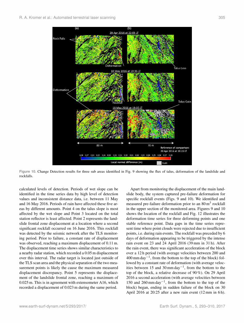
Figure 10. Change Detection results for three sub areas identified in Fig. 9 showing the flux of talus, deformation of the landslide androckfalls.

calculated levels of detection. Periods of wet slope can beidentified in the time series data by high level of detectionvalues and inconsistent distance data, i.e. between 11 Mayand 16 May 2016. Periods of rain have affected these five ar-eas by different amounts. Point 4 on the talus slope is mostaffected by the wet slope and Point 3 located on the totalstation reflector is least affected. Point 2 represents the land-slide frontal zone displacement at a location where a secondsignificant rockfall occurred on 16 June 2016. This rockfallwas detected by the seismic network after the TLS monitor-ing period. Prior to failure, a constant rate of displacementwas observed, reaching a maximum displacement of 0.11 m.The displacement time series shows similar characteristics toa nearby radar station, which recorded a 0.05 m displacementover this interval. The radar target is located just outside ofthe TLS scan area and the physical separation of the two mea-surement points is likely the cause the maximum measureddisplacement discrepancy. Point 5 represents the displace-ment of the landslide frontal zone, reaching a maximum of0.025 m. This is in agreement with extensometer A16, whichrecorded a displacement of 0.023 m during the same period.

Apart from monitoring the displacement of the main land-slide body, the system captured pre-failure deformation forspecific rockfall events (Figs. 9 and 10). We identified andmeasured pre-failure deformation prior to an 80 m3 rockfallin the upper section of the monitored area. Figures 9 and 10shows the location of the rockfall and Fig. 12 illustrates thedeformation time series for three deforming points and onestable reference point. Data gaps in the time series repre-sent time where point clouds were rejected due to insufficientpoints, i.e. during rain events. The rockfall was preceded by 6days of deformation appearing to be triggered by the intenserain event on 23 and 24 April 2016 (39 mm in 31 h). Afterthe rain event, there was significant acceleration of the blockover a 12 h period (with average velocities between 200 and400 mm day−1, from the bottom to the top of the block) fol-lowed by a constant rate of deformation (with average veloc-ities between 15 and 30 mm day−1, from the bottom to thetop of the block, a relative decrease of 90 %). On 29 April2016 a second acceleration (with average velocities between150 and 260 mm day−1, from the bottom to the top of theblock) began, ending in sudden failure of the block on 30April 2016 at 20:25 after a new rain event (12 mm in 6 h).



0

0.01

0.02

0.03

0.04

0.05

-0.1

-0.05

0

0.05

0.1

Apr 21

Apr 25

Apr 29

May 03

May 07

May 11

May 15

May 19

Apr 21

Apr 25

Apr 29

May 03

May 07

May 11

May 15

May 19

Leve

l of d

etec

�on

(m)

Loca

l nor

mal

diff

eren

ce (m

)

Pt.1

Pt.2

Pt.4

Pt.3

Pt.5

Displacement from closest radar target

Displacement measured using total sta�on

-0.1

-0.05

0

0.05

0.1

-0.1

-0.05

0

0.05

0.1

-0.1

-0.05

0

0.05

0.1

-0.1

-0.05

0

0.05

0.1

Loca

l nor

mal

diff

eren

ce (m

)Lo

cal n

orm

al d

iffer

ence

(m)

Loca

l nor

mal

diff

eren

ce (m

)Lo

cal n

orm

al d

iffer

ence

(m)

0

0.01

0.02

0.03

0.04

0.05

0

0.01

0.02

0.03

0.04

0.05

0

0.01

0.02

0.03

0.04

0.05

0

0.01

0.02

0.03

0.04

0.05

Leve

l of d

etec

�on

(m)

Leve

l of d

etec

�on

(m)

Leve

l of d

etec

�on

(m)

Leve

l of d

etec

�on

(m)

Figure 11. Distance and associated level of detection time seriesfor points of interest 1 to 5 marked in Fig. 8. Point 1, 3 and 4 rep-resent areas of the slope with non-detectable change. Point 2 repre-sents the pre-failure deformation of a rockfall that occurred on the16 June 2016 and Point 5 represents the deformation of the frontalzone of the landslide. Point 2 includes a comparison with measure-ments taken from the closest reference target and Point 3 includesa comparison with measurements taken with a total station for thesame target area.

The exact time of the event was extracted from the microseis-mic system record of the rockfall event. The maximum totaldeformation of the block reached 0.30 m (Point 3) to 0.45 m(Point 1) prior to block detachment. The movement of thethree points illustrated in Fig. 12 describes a local block top-pling failure, characterized by larger deformation at the topof the unstable block and smaller at the bottom.

5 Discussion

We presented an automatic processing TLS monitoring sys-tem which we have deployed at an active landslide site. Thesystem allows the study of earth surface processes at un-precedented levels of temporal detail and opens the door forstudying processes at the super-temporal level (multiple ac-quisitions per day) for long time intervals. The system is wellsuited for landslide and rock slope deformation monitoringand early warning systems and can also be adapted to studymany other earth surface processes. The automated scanningand automatic processing requires little input from users andprovides processed results in near-real time. This is of greatbenefit to decision makers in early warning scenarios, wheretime is an important resource.

For early warning monitoring the system can be a cost-effective, small and portable alternative to GB-InSAR sys-tems. It also offers significant spatial and temporal detail ofother slope processes allowing the calculation of volumesand vector deformation (Abellán et al., 2009; Oppikofer etal., 2009). TLS systems also have the benefit of being easyto transport and set up. For temporary early warning mon-itoring scenarios, such as remediation of a rockslide alonga transportation corridor, for example, TLS can be set upquickly using a portable power source (generators or bat-teries) and allow for results to be available directly on sitewithout the need to transfer data to a remote server. This isespecially beneficial in remote areas with no communicationinfrastructure, which is often the case in remote mountainousareas. The scanner can also be moved and resume scanningat a later date, unlike GB-InSAR, which suffers from phasedecorrelation.

We achieved a distance uncertainty range of 10 to 11 mmfor rock sections of the slope during favourable weatherconditions, an improvement compared to an uncertainty of25 mm achieved by Kasperski et al. (2010) at this study siteusing a Riegl LMS Z420i TLS. We did not achieve theoreti-cal improvement in our ability to detect change using 4-D fil-tering as discussed in Kromer et al. (2015). The critical factoris changing systematic errors over time caused by a combi-nation of influences such as atmospheric conditions, internalheating of the scanner and misalignment errors. Misalign-ment errors varied over time and were observed to be higherwhere total number of returns were reduced due to poor at-mospheric conditions. Improvements to the detection levelsachieved here could be reached by using scanners with wave-lengths less affected by atmospheric conditions and by usinga TLS system with a built-in scanner temperature correction.A survey design where a scanner is closer to the target of in-terest would also improve detection levels. Furthermore, al-ternative registration strategies may offer an improvement tothe registration error term, for example the stable area detec-tion registration algorithm proposed by Wujanz et al. (2016).For the observed phenomena at this site, however, a mil-limetre level of detection was not necessary over the 30 min



Figure 12. Pre-failure deformation of 80 m3 rockfall. (a) Location of 80 m3 rockfall. (b) Point cloud with mapped change showing defor-mation of the rock block prior to failure and four points used to plot time series data. Points A, B and C are located on the deforming areaand Point D is located on an adjacent stable area of slope. (c) Deformation time series (cumulative values) of three points on the surface ofthe deforming rock block and a nearby stable point. (d) Average 24 h velocity for Points A, B and C.

intra-scan interval. The observed pre-failure deformation forthe discrete rockfall event, for example, exhibited centimetrelevels of displacement prior to failure and the displacementof the landslide was in the centimetre range over the study’stime interval.

Atmospheric conditions including rain and changing sur-face reflectivity levels had a significant impact on the qual-ity of data collected using the Optech long-range TLS witha 1064 nm wavelength. At this study site, the missing datapoints caused by rain did not significantly affect our interpre-tation of slope processes. Displacement of the landslide oc-curred over a longer temporal scale and small data gaps hada low impact on our ability to interpret slope deformations.Furthermore, displacement of the landslide tended to be de-layed after rainfall. This effect has been observed by previousstudies at this site (Helmstetter and Garambois, 2010; Valletet al., 2015) and is believed to be due to the time it takes waterto infiltrate and build pressure in the subsurface. For the caseof the pre-failure deformation of the rockfall, the missed datapoints also did not affect the interpretation of the pre-failurestage.

This system was effective in monitoring the deformationof a deep-seated landslide automatically over a 6-week pe-riod of time. The detected deformation pattern in this case,greater movement at the top of the frontal zone comparedto the bottom, is in agreement with the hypothesis of a top-pling failure mechanism towards the valley (Kasperski et al.,2010b). The system was also successful in detecting pre-failure deformation of an 80 m3 rockfall event and of a signif-icant rockfall event that occurred after the monitoring periodon 16 June 2016 from the frontal zone. The former rock-fall appears to have been triggered by the rain episode from22 April to 24 April 2016 and showed multiple accelerationphases before collapse. The period over which deformationoccurred was only 6 days and may not have been capturedusing multi-temporal monitoring. A potential limitation oflong-term monitoring with TLS is the limited operational lifeof the laser, which is not reported by the manufacturers oflaser scanners.

We showed that this system can be beneficial for long-termmonitoring of a landslide and for detecting the pre-failurestage of rockfalls. Although this study was applied to a land-



slide site, the system developed herein can be adapted forwider applications for earth and ecological sciences, as dis-cussed in Eitler et al. (2016). This system will allow the un-derstanding, modelling and prediction of previously imper-ceptible earth changes.

6 Conclusions

In this study, we presented a near-real-time terrestrial laserscanner monitoring system that was tested on an active land-slide in the French Alps. The system was designed to col-lect data in an automated fashion and process data automat-ically in near-real time. The system was tested for a 6-weekperiod and captured flux of talus, displacement of the land-slide, pre-failure deformation of rockfalls including 6 daysof pre-failure deformation prior to an 80 m3 event. We werealso able to assess the effect of environmental influences ondata quality obtained with our scanner and defined a spatio-temporal confidence interval to estimate the variability inpoint cloud distance measurement uncertainty in space andtime.

We found that the TLS system can be an effective tool inmonitoring landslides and rockfall processes despite some ofits limitations. These include missing points due to poor at-mospheric conditions and changing slope reflectivity levels.At this study site, we observed slope deformation occurringover a longer period compared to the duration of the rainevents and that there appeared to be a delay between the rainevent and onset of increased slope deformation. For earlywarning monitoring of landslides, we showed that the systemcan be a suitable alternative to GB-InSAR deformation mon-itoring. The benefit of using this TLS system for landslidemonitoring is that it can be easily transported, set up quickly,a portable power source can be used, data can be processed inremote areas in the field automatically and results would bemade available in near-real time for on-site decision makers.Most importantly, we showed that TLS can be an effectivesystem for long-term high-temporal-resolution acquisitions.The system solves the problem of manually managing andprocessing large numbers of TLS data and opens the door tofuture study of earth processes at high levels of temporal de-tail. Future use of high-temporal-resolution TLS monitoringof earth surface processes will greatly increase our under-standing of previously imperceptible levels of earth change.

Data availability. The raw data can be requested from the GroupeRisque Rocheux et Mouvements de Sols (RRMS), Cerema Centre-Est, France.

The Supplement related to this article is available onlineat doi:10.5194/esurf-5-293-2017-supplement.

Competing interests. The authors declare that they have no con-flict of interest.

Acknowledgements. We would like to acknowledge the Centrefor studies and expertise on Risks, Environment, Mobility, andUrban and Country (Cerema) for supporting the research. Thefirst author would like to acknowledge support from the NaturalSciences and Engineering Research Council of Canada (NSERC)through the post-graduate scholarship programme. The secondauthor would like to acknowledge the support received from theH2020 Program of the European Commission under the MarieSkłodowska-Curie Individual Fellowships (MSCA-IF-2015-705215). We would also like to acknowledge Nick Rosser forhelpful advice on atmospheric correction and Antoine Guerin forhelp with field data collection.

Edited by: A. EltnerReviewed by: R. Salvini and one anonymous referee

References

Abellán, A., Jaboyedoff, M., Oppikofer, T., and Vilaplana, J. M.:Detection of millimetric deformation using a terrestrial laserscanner: experiment and application to a rockfall event, Nat.Hazards Earth Syst. Sci., 9, 365–372, doi:10.5194/nhess-9-365-2009, 2009.

Abellán, A., Calvet, J., Vilaplana, J. M., and Blanchard, J.: De-tection and spatial prediction of rockfalls by means of terres-trial laser scanner monitoring, Geomorphology, 119, 162–171,doi:10.1016/j.geomorph.2010.03.016, 2010.

Abellán, A., Carrea, D., Jaboyedoff, M., and Royan, M. J.: LiDARpoint cloud comparison: evaluation of denoising techniques us-ing 3D moving windows, in: EGU General Assembly – Geophys-ical Research Abstracts, 15, p. 11884, 2013.

Abellán, A., Oppikofer, T., Jaboyedoff, M., Rosser, N. J., Lim,M., and Lato, M. J.: Terrestrial laser scanning of rockslope instabilities, Earth Surf. Process. Landforms, 39, 80–97,doi:10.1002/esp.3493, 2014.

Adams, M., Gleirscher, E., and Gigele, T.: Automated TerrestrialLaser Scanner measurements of small-scale snow avalanches,Proc. Intern. Snow Science Workshop Grenoble-ChamonixMontBlanc, 2013.

Avian, M., Kellerer-Pirklbauer, A., and Bauer, A.: LiDAR for moni-toring mass movements in permafrost environments at the cirqueHinteres Langtal, Austria, between 2000 and 2008, Nat. HazardsEarth Syst. Sci., 9, 1087–1094, doi:10.5194/nhess-9-1087-2009,2009.

Barbarella, M.: Monitoring of large landslides by Terrestrial LaserScanning techniques: field data collection and processing, Eu-JRS, 126–151, doi:10.5721/EuJRS20134608, 2013.

Baudement, C., Bertrand, C., Guglielmi, Y., Viseur, S., Vallet, A.and Cappa, F.: Quantification de la dégradation mécanique etchimique d’un versant instable: approche géologique, hydromé-canique et hydrochimique Etude du versant instable de Séchili-enne, Isère (38), JAG-3èmes journées Aléas Gravitaires, 1–6,2013.


http://dx.doi.org/10.5194/esurf-5-293-2017-supplement

http://dx.doi.org/10.5194/nhess-9-365-2009


http://dx.doi.org/10.1016/j.geomorph.2010.03.016

http://dx.doi.org/10.1002/esp.3493


http://dx.doi.org/10.5721/EuJRS20134608


Bremer, M. and Sass, O.: Combining airborne and terres-trial laser scanning for quantifying erosion and deposi-tion by a debris flow event, Geomorphology, 138, 49–60,doi:10.1016/j.geomorph.2011.08.024, 2012.

Chanut, M.-A., Dubois, L., Duranthon, J.-P., and Durville, J.-L.:Mouvement de versant de Séchilienne : relations entre précipi-tations et déplacements, Tunisie, 14–16, 2013.

Chen, Y. and Medioni, G.: Object modelling by registration ofmultiple range images, Image Vision Comput., 10, 145–155,doi:10.1016/0262-8856(92)90066-C, 1992.

Ciddor, P. E.: Refractive index of air: new equations forthe visible and near infrared, Appl. Opt., 35, 1566–1573,doi:10.1364/AO.35.001566, 1996.

Corominas, J., van Westen, C., Frattini, P., Cascini, L., Malet, J. P.,Fotopoulou, S., Catani, F., Van Den Eeckhaut, M., Mavrouli, O.,Agliardi, F., Pitilakis, K., Winter, M. G., Pastor, M., Ferlisi, S.,Tofani, V., Hervás, J., and Smith, J. T.: Recommendations for thequantitative analysis of landslide risk, B. Eng. Geol. Environ.,73, 209–263, doi:10.1007/s10064-013-0538-8, 2014.

Dewitte, O., Jasselette, J. C., Cornet, Y., Van Den Eeckhaut, M.,Collignon, A., Poesen, J., and Demoulin, A.: Tracking land-slide displacements by multi-temporal DTMs: A combined aerialstereophotogrammetric and LIDAR approach in western Bel-gium, Eng. Geol., 99, 11–22, doi:10.1016/j.enggeo.2008.02.006,2008.

Dubois, L., chanut, M.-A., and Duranthon, J.-P.: Amélioration con-tinue des dispositifs d’auscultation et de surveillance intégrésdans le suivi du versant instable des Ruines de Séchilienne, Géo-logue, 183, 50–55, 2014.

Dunner, C., Klein, E., and Bigarre, P.: Monitoring multi-paramètresdu mouvement de versant des Ruines de Séchilienne (Isère, 38),Journées “Aléa gravitaire”(JAG 2011), 2011.

Duranthon, J. P.: Le mouvement de versant rocheux de grande am-pleur des Ruines de Séchilienne–Surveillance Instrumentation,Journées Nationales de Géotechnique et Géologie de l’ingénieur(JNGG), 2006.

Eitel, J. U. H., Vierling, L. A., and Magney, T. S.: A lightweight, lowcost autonomously operating terrestrial laser scanner for quanti-fying and monitoring ecosystem structural dynamics, Agr. For-est Meteorol., 180, 86–96, doi:10.1016/j.agrformet.2013.05.012,2013.

Eitel, J. U. H., Höfle, B., Vierling, L. A., Abellán, A., Asner, G.P., Deems, J. S., Glennie, C. L., Joerg, P. C., LeWinter, A. L.,Magney, T. S., Mandlburger, G., Morton, D. C., Müller, J., andVierling, K. T.: Beyond 3-D: The new spectrum of lidar applica-tions for earth and ecological sciences, Remote Sens. Environ.,186, 372–392, doi:10.1016/j.rse.2016.08.018, 2016.

Evrard, H., Gouin, T., Benoit, A., and Duranthon Séchilienne, J.-P.:Risques majeurs d’éboulements en masse: Point sur la surveil-lance du site, Bull. Liaison Lab. Ponts Chaussees, 165, 7–16,1990.

Fey, C. and Wichmann, V.: Long-range terrestrial laser scan-ning for geomorphological change detection in alpine terrain–handling uncertainties, Earth Surf. Proc. Land., 4, 789–802,doi:10.1002/esp.4022, 2017.

Fischler, M. A. and Bolles, R. C.: Random sample consensus: aparadigm for model fitting with applications to image analysisand automated cartography, Communications of the ACM, 24,381–395, doi:10.1145/358669.358692, 1981.

Guglielmi, Y., Vengeon, J., Bertrand, C., Mudry, J., Follacci, J., andGiraud, A.: Hydrogeochemistry: an investigation tool to evalu-ate infiltration into large moving rock masses (case study of LaClapière and Séchilienne alpine landslides), B. Eng. Geol. Envi-ron., 61, 311–324, doi:10.1007/s10064-001-0144-z, 2002.

Helmstetter, A. and Garambois, S.: Seismic monitoring of Séchili-enne rockslide (French Alps): Analysis of seismic signals andtheir correlation with rainfalls, J. Geophys. Res.-Earth, 115, 1–15, doi:10.1029/2009JF001532, 2010.

Holz, D., Ichim, A. E., Tombari, F., Rusu, R. B., and Behnke, S.:Registration with the Point Cloud Library A Modular Frameworkfor Aligning in 3-D?, The Royal Society, 22, 110–124, 2015.

Jaboyedoff, M., Oppikofer, T., Abellán, A., Derron, M.-H.,Loye, A., Metzger, R., and Pedrazzini, A.: Use of LIDARin landslide investigations: a review, Nat Hazards, 61, 5–28,doi:10.1007/s11069-010-9634-2, 2012.

Kasperski, J.: Confrontation des données de terrain et de l’imageriemulti-sources pour la compréhension de la dynamique des mou-vements de versants, Université Claude Bernard – Lyon I, Lyon,8 February, 2008.

Kasperski, J., Delacourt, C., Allemand, P., Potherat, P., Jaud, M.,and Varrel, E.: Application of a Terrestrial Laser Scanner (TLS)to the Study of the Séchilienne Landslide (Isère, France), RemoteSensing 2011, 2, 2785–2802, doi:10.3390/rs122785, 2010.

Krautblatter, M. and Dikau, R.: Towards a uniform concept for thecomparison and extrapolation of rockwall retreat and rockfallsupply, Geografiska Annaler: Series A, Phys. Geogr., 89, 21–40,doi:10.1111/j.1468-0459.2007.00305.x, 2007.

Kromer, R. A., Hutchinson, D. J., Lato, M. J., Gauthier, D., and Ed-wards, T.: Identifying rock slope failure precursors using LiDARfor transportation corridor hazard management, Eng. Geol., 195,93–103, doi:10.1016/j.enggeo.2015.05.012, 2015a.

Kromer, R., Abellán, A., Hutchinson, D., Lato, M., Edwards, T.,and Jaboyedoff, M.: A 4D Filtering and Calibration Techniquefor Small-Scale Point Cloud Change Detection with a TerrestrialLaser Scanner, Remote Sensing 2011, 7, 13029–13052, 2015b.

Lague, D., Brodu, N., and Leroux, J.: Accurate 3D comparison ofcomplex topography with terrestrial laser scanner: Application tothe Rangitikei canyon (N-Z), ISPRS J. Photogramm., 82, 10–26,doi:10.1016/j.isprsjprs.2013.04.009, 2013.

Lato, M. J., Hutchinson, D. J., Gauthier, D., Edwards, T., and On-dercin, M.: Comparison of ALS, TLS and terrestrial photogram-metry for mapping differential slope change in mountainous ter-rain, Can. Geotech. J., 52, 129–140, doi:10.1139/cgj-2014-0051,2014.

Le Roux, O., Jongmans, D., Kasperski, J., Schwartz, S., Potherat, P.,Lebrouc, V., Lagabrielle, R., and Meric, O.: Deep geophysicalinvestigation of the large Séchilienne landslide (Western Alps,France) and calibration with geological data, Eng. Geol., 120,18–31, doi:10.1016/j.enggeo.2011.03.004, 2011.

Levenberg, K.: A method for the solution of certain non-linear problems in least squares, Q. Appl. Math., 2, 164–168,doi:10.1090/qam/10666 , 1944.

Lichti, D. D. and Licht, M. G.: Experiences with terrestrial laserscanner modelling and accuracy assessment, Int. Arch. Pho-togramm. Remote Sens. Spat Inf. Sci., doi:10.7202/706354ar,2006.

Lichti, D. D., Gordon, S. J., and Tipdecho, T.: Error Modelsand Propagation in Directly Georeferenced Terrestrial Laser



http://dx.doi.org/10.1016/0262-8856(92)90066-C

http://dx.doi.org/10.1364/AO.35.001566

http://dx.doi.org/10.1007/s10064-013-0538-8

http://dx.doi.org/10.1016/j.enggeo.2008.02.006

http://dx.doi.org/10.1016/j.agrformet.2013.05.012

http://dx.doi.org/10.1016/j.rse.2016.08.018


http://dx.doi.org/10.1145/358669.358692

http://dx.doi.org/10.1007/s10064-001-0144-z

http://dx.doi.org/10.1029/2009JF001532

http://dx.doi.org/10.1007/s11069-010-9634-2

http://dx.doi.org/10.3390/rs122785

http://dx.doi.org/10.1111/j.1468-0459.2007.00305.x


http://dx.doi.org/10.1016/j.isprsjprs.2013.04.009

http://dx.doi.org/10.1139/cgj-2014-0051


http://dx.doi.org/10.1090/qam/10666

http://dx.doi.org/10.7202/706354ar


Scanner Networks, Journal of Surveying Engineerin, 131,135–142, surveying engineering, doi:10.1061/(ASCE)0733-9453(2005)131:4(135), 2005.

Lim, M., Petley, D. N., Rosser, N. J., Allison, R. J., Long,A. J., and Pybus, D.: Combined Digital Photogrammetry andTime-of-Flight Laser Scanning for Monitoring Cliff Evolution,Photogrammetric Record, 20, 109–129, doi:10.1111/j.1477-9730.2005.00315.x, 2005.

Marquardt, D. W.: An algorithm for least-squares estimation of non-linear parameters, J. Soc. Ind. Appl. Math. 11, 431–441, 1963.

Metternicht, G., Hurni, L., and Gogu, R.: Remote sens-ing of landslides: An analysis of the potential contribu-tion to geo-spatial systems for hazard assessment in moun-tainous environments, Remote Sens. Environ., 98, 284–303,doi:10.1016/j.rse.2005.08.004, 2005.

Milan, D. J., Heritage, G. L., and Hetherington, D.: Application ofa 3D laser scanner in the assessment of erosion and depositionvolumes and channel change in a proglacial river, Earth Surf.Proc. Land., 32, 1657–1674, doi:10.1002/esp.1592, 2007.

Monserrat, O. and Crosetto, M.: Deformation measurement us-ing terrestrial laser scanning data and least squares 3Dsurface matching, ISPRS J. Photogramm., 63, 142–154,doi:10.1016/j.isprsjprs.2007.07.008, 2008.

Muja, M. and Lowe, D. G.: Fast Approximate Nearest Neighborswith Automatic Algorithm Configuration, VISAPP, 2009.

Oppikofer, T., Jaboyedoff, M., and Keusen, H.-R.: Collapse at theeastern Eiger flank in the Swiss Alps, Nat. Geosci., 1, 531–535,doi:10.1038/ngeo258, 2008.

Oppikofer, T., Jaboyedoff, M., Blikra, L., Derron, M.-H., and Met-zger, R.: Characterization and monitoring of the Åknes rockslideusing terrestrial laser scanning, Nat. Hazards Earth Syst. Sci., 9,1003–1019, doi:10.5194/nhess-9-1003-2009, 2009.

Orem, C. A. and Pelletier, J. D.: Quantifying the time scale ofelevated geomorphic response following wildfires using multi-temporal LiDAR data: An example from the Las Conchas fire,Jemez Mountains, New Mexico, Geomorphology, 232, 224–238,doi:10.1016/j.geomorph.2015.01.006, 2015.

Pothérat, P. and Alfonsi, P.: Les mouvements de versant de Séchili-enne (Isère). Prise en compte de l’héritage structural pour leursimulation numérique, Revue française de géotechnique, 95–96,2001.

Rosser, N. J., Petley, D. N., Lim, M., Dunning, S. A., and Allison, R.J.: Terrestrial laser scanning for monitoring the process of hardrock coastal cliff erosion, Q. J. Eng. Geol. Hydrogeol., 38, 363–375, doi:10.1144/1470-9236/05-008, 2005.

Royán, M. J., Abellán, A., Jaboyedoff, M., Vilaplana, J. M., andCalvet, J.: Spatio-temporal analysis of rockfall pre-failure de-formation using Terrestrial LiDAR, Landslides, 11, 697–709,doi:10.1007/s10346-013-0442-0, 2013.

Royán, M. J., Abellán, A., and Vilaplana, J. M.: Progres-sive failure leading to the 3 December 2013 rockfall atPuigcercós scarp (Catalonia, Spain), Landslides, 12, 585–595,doi:10.1007/s10346-015-0573-6, 2015.

Rusu, R. B. and Cousins, S.: 3D is here: Point Cloud Library (PCL),IEEE, 1–4, 2011.

Rusu, R. B., Blodow, N., and Beetz, M.: Fast point feature his-tograms (FPFH) for 3D registration, in: IEEE International Con-ference on Robotics and Automation (ICRA), 1848–1853, 2009.

Schürch, P., Densmore, A. L., Rosser, N. J., Lim, M., and McArdell,B. W.: Detection of surface change in complex topographyusing terrestrial laser scanning: application to the Illgrabendebris-flow channel, Earth Surf. Proc. Land., 36, 1847–1859,doi:10.1002/esp.2206, 2011.

Teledyne Optech: ILRIS Terrestrial Laser Scanner, availableat: http://www.teledyneoptech.com/wp-content/uploads/ILRIS-Spec-Sheet-140730-WEB.pdf (last access: 15 Jan-uary 2017), 2014a.

Teledyne Optech: Optech ILRIS Command Line User Manual,2014b.

Teza, G., Galgaro, A., Zaltron, N., and Genevois, R.: Terres-trial laser scanner to detect landslide displacement fields:a new approach, Int. J. Remote Sensing, 28, 3425–3446,doi:10.1080/01431160601024234, 2007.

Travelletti, J., Oppikofer, T., and Delacourt, C.: Monitoring land-slide displacements during a controlled rain experiment us-ing a long-range terrestrial laser scanning (TLS), InternationalArchives of Photogrammetry and Remote Sensing, 2008.

Vallet, A., Charlier, J. B., Fabbri, O., Bertrand, C., Carry, N.,and Mudry, J.: Functioning and precipitation-displacement mod-elling of rainfall-induced deep-seated landslides subject to creepdeformation, Landslides, 13, 653–670, doi:10.1007/s10346-015-0592-3, 2015.

Vulliez, C.: Apports des méthodes d’imagerie 3D pour la caractéri-sation et le monitoring du glissement rocheux de Séchilienne(Vallée de la Romanche, Isère, France), Lausanne, 12 February,1–123, 2016.

Wang, C.-K. and Lu, Y.-Y.: Potential of ILRIS3D Intensity Datafor Planar Surfaces Segmentation, Sensors, 9, 5770–5782,doi:10.3390/s90705770, 2009.

Wujanz, D., Krueger, D., and Neitzel, F.: Identification of Stable Ar-eas in Unreferenced Laser Scans for Deformation Measurement,Photogramm. Rec., 31, 261–280, 2016.

Zhong, Y.: Intrinsic shape signatures: A shape descriptor for 3Dobject recognition, IEEE, 689–696, 2009.


http://dx.doi.org/10.1061/(ASCE)0733-9453(2005)131:4(135)

http://dx.doi.org/10.1061/(ASCE)0733-9453(2005)131:4(135)

http://dx.doi.org/10.1111/j.1477-9730.2005.00315.x

http://dx.doi.org/10.1111/j.1477-9730.2005.00315.x

http://dx.doi.org/10.1016/j.rse.2005.08.004


http://dx.doi.org/10.1016/j.isprsjprs.2007.07.008

http://dx.doi.org/10.1038/ngeo258



http://dx.doi.org/10.1144/1470-9236/05-008

http://dx.doi.org/10.1007/s10346-013-0442-0

http://dx.doi.org/10.1007/s10346-015-0573-6


http://www.teledyneoptech.com/wp-content/uploads/ILRIS-Spec-Sheet-140730-WEB.pdf

http://www.teledyneoptech.com/wp-content/uploads/ILRIS-Spec-Sheet-140730-WEB.pdf

http://dx.doi.org/10.1080/01431160601024234

http://dx.doi.org/10.1007/s10346-015-0592-3

http://dx.doi.org/10.1007/s10346-015-0592-3

http://dx.doi.org/10.3390/s90705770

automated terrestrial laser scanning with near-real … terrestrial laser scanning with near ... and...

Documents