automatic arrhythmia classification: a pattern …...automatic arrhythmia classification: a pattern...
TRANSCRIPT

Automatic Arrhythmia Classification:
A Pattern Recognition Approach
Diana Paiva Moreira Batista
Thesis to obtain the Master of Science Degree in
Biomedical Engineering
Supervisors: Prof. Ana Luísa Nobre Fred, Dr. Rui Cruz Ferreira
Examination Committee
Chairperson: Prof. Paulo Rui Alves Fernandes
Supervisor: Prof. Ana Luísa Nobre Fred
Members of the Committee: Prof. Maria Margarida Campos da Silveira
Dr. Eduardo Antunes
November 2014

II

III
Acknowledgments
A few people were fundamental to the successful elaboration of this work and I use this section to
acknowledge their contribution.
First, I thank Dr. Eduardo Antunes for the enthusiasm towards this project. I thank him for his
availability and willingness to share his medical expertise, as well as the efforts made to organize ECG
acquisition sessions at the Hospital de Santa Marta.
Thanks to the medical and technical staff at the Hospital de Santa Marta, for providing me all the help
necessary during the acquisitions. A special mention to Sofia Silva, whose unparalleled patience and
availability even during the busier days were much appreciated.
I thank Dr. Rui Cruz Ferreira for his guidance.
Last but not least, I thank my supervisor, Ana Fred, for the knowledge transmitted, the ideas shared,
and the advice given during the elaboration of this thesis.

IV

V
Resumo
Nas últimas décadas tem-se assistido ao contínuo desenvolvimento de aparelhos de monitorização
cardíaca. A quantidade de dados recolhida é portanto cada vez maior e torna-se necessário
desenvolver algoritmos que auxiliem a sua análise, automatizando-a sempre que possível. A
identificação de ritmos a partir de registos electrocardiográficos (ECGs) é parte importante deste
problema e pode ser abordada utilizando técnicas de reconhecimento de padrões.
Este estudo focou-se no processamento de ECGs, dando particular ênfase à classificação automática
de arritmias. Utilizaram-se características espectrais, extraídas recorrendo à transformação de
wavelet, e características temporais. Comparou-se o desempenho de três classificadores: k-vizinhos
mais próximos, perceptrão multi-camada e máquina de vectores de suporte (SVM, do inglês Support
Vector Machine). O método proposto foi validado recorrendo a uma reconhecida base de dados. Foi
ainda possível efectuar testes iniciais com ECGs adquiridos nos dedos com o sistema BITalino.
Na distinção entre ritmo sinusal e fibrilação auricular o melhor classificador foi o SVM, que atingiu
uma taxa global de exactidão de 99.08%. Este resultado foi obtido com uma combinação de
características espectrais e temporais pelo que nas experiências com múltiplas classes se utilizaram
estas mesmas características. Considerando oito ritmos, divididos em cinco classes, foi possível
atingir uma exactidão próxima de 94%. Os testes iniciais realizados com aquisições do BITalino
provaram que também é possível classificar automaticamente, com sucesso, ECGs adquiridos com
este sistema.
Palavras-chave: Arritmia, Reconhecimento de Padrões, Redes Neuronais, k-Vizinhos Mais
Próximos, Máquina de Vectores de Suporte

VI

VII
Abstract
With the continuous development of tools for cardiac monitoring, an enormous amount of data can be
collected and has to be analyzed. It is therefore crucial to develop new algorithms that will aid in the
analysis of electrocardiograms (ECGs), automatizing, to a certain extent, the process. The recognition
of arrhythmias is one important part of the problem and pattern recognition methods have been
successfully employed.
In this work, a methodology for ECG analysis was presented. The main focus was on automatic
arrhythmia classification. Both spectral features, extracted using the wavelet transform, and time
domain parameters were considered for classification. The performance of three supervised learning
classifiers was compared: k-nearest neighbor, multilayer perceptron and support vector machine
(SVM). Validation of the proposed method was performed resorting to benchmarked data from a
widely used arrhythmia database. Additionally, initial experiments were carried out to assess the
feasibility of classifying ECG records acquired with the BITalino system at the fingers.
An overall accuracy of 99.08% was achieved with the SVM classifier when distinguishing between
normal sinus rhythm and the most common arrhythmia, atrial fibrillation. A feature set containing a
combination of spectral and time domain parameters proved to be the most suitable choice and was
then used in multiclass experiments. Classification of eight types of rhythms, divided in five classes,
was achieved with a correct classification rate close to 94%. The initial experiments carried out with
records from the BITalino attested the possibility of automatically classifying ECGs acquired with this
device.
Keywords: Arrhythmia, ECG, Pattern Analysis, Artificial Neural Network, k-Nearest Neighbors,
Support Vector Machine

VIII
Table of Contents
Acknowledgments ................................................................................................................................... III
Resumo ................................................................................................................................................... V
Abstract.................................................................................................................................................. VII
List of Figures ......................................................................................................................................... XI
List of Tables ......................................................................................................................................... XV
List of Acronyms .................................................................................................................................. XVII
1. Introduction ........................................................................................................................................... 1
1.1 Motivation.................................................................................................................................... 1
1.2 Goals and Proposed Approach .................................................................................................. 1
1.3 Contributions ............................................................................................................................... 2
1.4 Structure ..................................................................................................................................... 2
2. Electrophysiology and Cardiac Monitors .............................................................................................. 3
2.1 Electrical Conduction System of the Heart ................................................................................. 3
2.2 Electrocardiogram ....................................................................................................................... 4
2.3 Arrhythmias and Conduction Abnormalities ............................................................................... 5
2.3.1 Sinus Node Rhythms ....................................................................................................... 5
2.3.2 Atrial Arrhythmias ............................................................................................................. 7
2.3.3 Junctional Arrhythmias and Atrioventricular Blocks ......................................................... 9
2.3.4 Ventricular Arrhythmias and Bundle-Branch Blocks ......................................................10
2.4 Cardiac Monitors .......................................................................................................................14
2.4.1 Standard 12-Lead ECG .................................................................................................14
2.4.2 Ambulatory ECG Monitoring Systems ...........................................................................14
3. State-of-the-Art ...................................................................................................................................19
3.1 Review of Beat / Rhythm Classification ....................................................................................19
3.2 Wavelet Transform ...................................................................................................................26
3.3 Power Spectral Density ............................................................................................................27
3.4 Classifiers .................................................................................................................................28
3.4.1 k-Nearest Neighbors ......................................................................................................28
3.4.2 Multilayer Perceptrons ...................................................................................................29
3.4.3 Support Vector Machines ...............................................................................................31

IX
4. Methodology .......................................................................................................................................33
4.1 Signal Acquisition and Processing ...........................................................................................33
4.1.1 BITalino system ..............................................................................................................33
4.1.2 Filtering ..........................................................................................................................34
4.1.3 R peak detection ............................................................................................................34
4.2 Feature Extraction ....................................................................................................................36
4.2.1 Spectral Parameters ......................................................................................................36
4.2.2 Time Domain Parameters ..............................................................................................39
4.3 Feature Normalization ..............................................................................................................39
4.4 Classifiers .................................................................................................................................40
4.5 Validation Setup ........................................................................................................................41
5. Experimental Setup and Results ........................................................................................................43
5.1 Experimental Setup ..................................................................................................................43
5.1.1 BITalino Acquisitions ......................................................................................................43
5.1.2 Benchmark Data ............................................................................................................44
5.2 Results R Peak Detection .........................................................................................................45
5.3 Rhythm Classification on Benchmark Database ......................................................................48
5.3.1 Database Assembly .......................................................................................................48
5.3.2 Normal Sinus Rhythm vs. Atrial Fibrillation ....................................................................49
5.3.3 Multiple Rhythms............................................................................................................62
5.4. Rhythm Classification with BITalino Acquisitions ....................................................................71
6. Conclusions and Future Work ............................................................................................................74
References .............................................................................................................................................76
Annex A ..................................................................................................................................................81
Annex B ..................................................................................................................................................82

X

XI
List of Figures
Figure 1: Elements of the cardiac electrical conduction system (Williams, 2010). ................................. 3
Figure 2: Basic components of the ECG complex (Huff, 2006). ............................................................. 4
Figure 3: Four arrhythmogenic zones (Garcia and Miller, 2004). ............................................................ 5
Figure 4: Recording of a normal sinus rhythm ECG. .............................................................................. 6
Figure 5: ECG showing a premature atrial contraction with an underlying sinus bradycardia rhythm.... 7
Figure 6: Recording of atrial fibrillation. ................................................................................................... 8
Figure 7: Recording of junctional escape rhythm. ................................................................................... 9
Figure 8: Rhythm strips of a LBBB. ....................................................................................................... 11
Figure 9: ECG showing a bigeminal rhythm. ......................................................................................... 11
Figure 10: Lead placement for a 12-lead ECG (Garcia and Miller, 2004). ............................................ 14
Figure 11: Philips DigiTrak XT Holter Recorder (Philips, 2014) ............................................................ 15
Figure 12: Reveal XT insertable cardiac monitor device from Medtronic (Medtronic, 2014). ............... 16
Figure 13: Mobile Cardiac Outpatient Telemetry system from CardioNet (CardioNet, 2014) ............... 16
Figure 14: Left: ZIO XT Patch monitoring process (iRhythm, 2014); Right: Overview of the Corventis
NUVANT/PiiX system (Lobodzinski et al., 2013). ................................................................................. 17
Figure 15: Alivecor system (Lau et al., 2013) ........................................................................................ 18
Figure 16: Mallat’s algorithm for discrete wavelet decomposition (Martínez et al., 2004). ................... 27
Figure 17: Schematic representation of the splitting of the signal. ....................................................... 27
Figure 18: Example of kNN binary classification problem. Two features are used to distinguish
between class 1, blue circles, and class 2, red triangles. When 3 neighbors are used for classification
the test sample (green square) is assigned to class 2. ......................................................................... 28
Figure 19: A multilayer perceptron with 2 neurons in the input layer, 3 in the hidden layer and 2 in the
output layer. ........................................................................................................................................... 29
Figure 20: Basic architecture of a neuron with 4 inputs including one bias term. The sum of the inputs
is then passed through a nonlinear function S. ..................................................................................... 29
Figure 21: Example of a SVM binary classification problem. Highlighted in green are the three support
vectors. Continuous and dashed lines represent respectively decision boundary and margins. .......... 31
Figure 22: Automatic signal analysis methodology. .............................................................................. 33
Figure 23: Steps of the classification task. ............................................................................................ 33
Figure 24: BITalino system used for ECG acquisitions. ........................................................................ 33
Figure 25: 10 seconds extract of an ECG acquired with the BITalino. Raw (left) and filtered (right)
records are shown. ................................................................................................................................ 34
Figure 26: Schematic representation of the R peak detection algorithm. Adapted from (Hamilton,
2002). ..................................................................................................................................................... 35
Figure 27: Result of the R peak detection algorithm on a normal sinus rhythm ECG. ......................... 36
Figure 28: Feature extraction process of the spectral parameters........................................................ 36
Figure 29: Mother wavelet and scaling function of the quadratic spline wavelet. ................................. 37
Figure 30: 10 seconds extract of a normal sinus rhythm ECG. ............................................................. 37

XII
Figure 31: Approximation (A6) and detail (D1 to D6) coefficients of the wavelet decomposition of a 10
seconds normal sinus rhythm ECG. ...................................................................................................... 38
Figure 32: PSD of each one of the approximation (A6) and detail (D1 to D6) wavelet coefficients.
Dotted red lines delimitate the sub-bands of feature set A. .................................................................. 38
Figure 33: Distinction between normal sinus rhythm (N) and atrial fibrillation (AFIB) segments
according to normalized average and standard deviation of RR intervals. ........................................... 39
Figure 34: Example of the topology of a network with 2 input features, 3 hidden neurons and 2
outputs. .................................................................................................................................................. 40
Figure 35: Scheme for training and testing the classifier. ..................................................................... 41
Figure 36: Ten seconds from a record of the MIT-BIH arrhythmia database. Each beat is individually
labeled and rhythm changes appear below beat annotations (preceded by ‘(‘) (Moody and Mark,
2001). ..................................................................................................................................................... 44
Figure 37: Sensitivity-positive predictive value curve for different threshold (TH) values. .................... 45
Figure 38: Example of two aberrated atrial premature beats (a) that were not detected by the
segmentation algorithm. ........................................................................................................................ 47
Figure 39: Example of one unclassifiable beat (Q) that was not detected by the segmentation
algorithm. ............................................................................................................................................... 47
Figure 40: Example of two false positive errors. In the left, where R peaks are inverted, a P wave is
detected. In the right, where PVCs occur, a T wave is detected........................................................... 48
Figure 41: Mean and standard deviation of the test error as a function of the number of neurons in the
hidden layer for the two normalization schemes, for feature set C. ...................................................... 49
Figure 42: Mean and standard deviation of the test error as a function of the number of neighbors
used for classification for the two normalization schemes, for feature set C. ....................................... 50
Figure 43: Heat map showing the accuracy of the SVM classifier for multiple values of C and gamma,
for feature set C. .................................................................................................................................... 50
Figure 44: Mean and standard deviation of the test error as a function of the number of neurons in the
hidden layer for the two normalization schemes, for feature set A. ...................................................... 52
Figure 45: Mean and standard deviation of the test error as a function of the number of neighbors
used for classification for the two normalization schemes, for feature set A. ....................................... 52
Figure 46: Heat map showing the accuracy of the SVM classifier for multiple values of C and gamma,
for feature set A. .................................................................................................................................... 52
Figure 47: Mean and standard deviation of the test error as a function of the number of neurons in the
hidden layer for the two normalization schemes, for feature set B. ...................................................... 53
Figure 48: Mean and standard deviation of the test error as a function of the number of neighbors
used for classification for the two normalization schemes, for feature set B. ....................................... 54
Figure 49: Heat map showing the accuracy of the SVM classifier for multiple values of C and gamma,
for feature set B. .................................................................................................................................... 54
Figure 50: Means and standard deviations of test errors for feature sets C (time parameters), A
(average PSD values) and B (large range power values). .................................................................... 55

XIII
Figure 51: Mean and standard deviation of the test error as a function of the number of neurons in the
hidden layer for the two normalization schemes, for feature set A + C. ................................................ 56
Figure 52: Mean and standard deviation of the test error as a function of the number of neighbors
used for classification for the two normalization schemes, for feature set A + C. ................................. 56
Figure 53: Heat map showing the accuracy of the SVM classifier for multiple values of C and gamma,
for feature set A + C. ............................................................................................................................. 56
Figure 54: Mean and standard deviation of the test error as a function of the number of neurons in the
hidden layer for the two normalization schemes, for feature set B + C. ................................................ 57
Figure 55: Mean and standard deviation of the test error as a function of the number of neighbors
used for classification for the two normalization schemes, for feature set B + C. ................................. 58
Figure 56: Heat map showing the accuracy of the SVM classifier for multiple values of C and gamma,
for feature set B + C. ............................................................................................................................. 58
Figure 57: Means and standard deviations of test errors for feature sets A + C and B + C. ................ 59
Figure 58: Mean and standard deviation of the test error as a function of the segments’ length. ........ 61
Figure 59: Comparison of rhythm classification error rate when using reference annotations and the
segmentation algorithm. ........................................................................................................................ 62

XIV

XV
List of Tables
Table 1: Main cardiac rhythms classified according to their origin. ....................................................... 13
Table 2: Types of beats and rhythms present in the MIT-BIH arrhythmia database............................. 44
Table 3: Sensitivity and positive predictive value of R peak detection according to the type of rhythm.
............................................................................................................................................................... 46
Table 4: Results of the R peak detection algorithm per beat type. ....................................................... 46
Table 5: Number of segments per rhythm type for different segment’s lengths. .................................. 48
Table 6: Best classifiers’ parameters for each classification task. ........................................................ 51
Table 7: Results obtained with feature set C......................................................................................... 51
Table 8: Results obtained with feature set A. ........................................................................................ 53
Table 9: Results obtained with feature set B. ........................................................................................ 55
Table 10: Results obtained with feature set A + C. ............................................................................... 57
Table 11: Results obtained with feature set B + C. ............................................................................... 58
Table 12: Results obtained when varying the segments’ length for the ANN classifier. ....................... 60
Table 13: Results obtained when varying the segments’ length for the kNN classifier. ....................... 60
Table 14: Results obtained when varying the segments’ length for the SVM classifier. ....................... 60
Table 15: Results obtained with feature set B + C using non-reference R peak annotations............... 62
Table 16: Results obtained with feature sets B + C in the distinction of three rhythms. ....................... 63
Table 17: Results obtained with feature sets B + C in the distinction of four rhythms. ......................... 64
Table 18: Results obtained with feature sets B + C in the distinction of four rhythms. ......................... 64
Table 19: Results obtained with feature sets B + C in the distinction of five rhythms (31 samples per
rhythm)................................................................................................................................................... 65
Table 20: Results obtained with feature sets B + C in the distinction of five rhythms (12 samples per
rhythm)................................................................................................................................................... 65
Table 21: Results obtained with feature sets B + C in the distinction of six rhythms (12 samples per
rhythm)................................................................................................................................................... 66
Table 22: Results obtained with feature sets B + C in the distinction of six classes (43 samples per
rhythm)................................................................................................................................................... 66
Table 23: Results obtained with feature sets B + C in the distinction of seven classes (60 samples per
rhythm)................................................................................................................................................... 68
Table 24: Results obtained with feature sets B + C in the distinction of six classes (68 samples per
rhythm)................................................................................................................................................... 68
Table 25: Results obtained with feature sets B + C in the distinction of five classes (68 samples per
rhythm)................................................................................................................................................... 69
Table 26: Results obtained with feature sets B + C in the distinction of five classes (68 samples per
rhythm)................................................................................................................................................... 70
Table 27: Results of Experiment A with filtered BITtalino records. ....................................................... 71
Table 28: Results of Experiment A with raw BITalino records. ............................................................. 72
Table 29: Results of Experiment B with filtered BITalino records. ........................................................ 72
Table 30: Results of Experiment B with raw BITalino records. ............................................................. 72
Table 31: ECG interpretation for the acquisitions with the BITalino System. ........................................ 82

XVI

XVII
List of Acronyms
AF Atrial Fibrillation
ANN Artificial Neural Network
AV Atrioventricular
bpm Beats per minute
ECG Electrocardiogram
kNN k-Nearest Neighbor
LAFB Left Anterior Fascicular Block
LBBB Left Bundle Branch Block
LGL Lown–Ganong–Levine
LPFB Left Posterior Fascicular Block
MLP Multilayer Perceptron
PAC Premature Atrial Contraction
PJC Premature Junctional Contraction
PSD Power Spectral Density
PVC Premature Ventricular Contraction
RBBB Right Bundle Branch Block
RDWT Redundant Discrete Wavelet Transform
SA Sinoatrial
SVM Support Vector Machine

XVIII

1
1. Introduction
1.1 Motivation
An electrocardiogram (ECG) is a recording of the heart’s electrical activity. This recording can be
obtained in a non-invasive manner, typically by placing electrodes on the surface of the chest. Besides
the standard 12-lead ECG, widely used in clinical practice, a number of other cardiac monitoring tools
have been developed in the last few decades. Portable ECG devices include Holter monitors, mobile
cardiac outpatient telemetry systems, event recorders and patch monitors. An enormous amount of
data can be collected by such devices and it is therefore essential to develop algorithms that aid in the
analysis of these records.
An arrhythmia is any disturbances in rate, rhythm, or conduction of the electrical impulse through the
heart. While some arrhythmias are harmless others can really compromise the cardiac output and be
potentially life threatening. Hence, the diagnosis of cardiac arrhythmias, which can be achieved by
analyzing ECG records, is an important medical topic.
Automatic analysis of ECG strips for the diagnosis of arrhythmias is an ongoing research. Numerous
algorithms have been proposed to classify beat or rhythm types. Some of these studies show
promising results but there is certainly room for improvement. Furthermore, the proposed algorithms
are sometimes tested on small and/or private databases, which hinder an objective validation.
1.2 Goals and Proposed Approach
The objective of this work is the automatic classification of cardiac rhythms from one-lead ECG
records. Ultimately, pervasive ECG acquisition, processing, and classification, is sought. Therefore, all
these steps are approached but main attention is given to the classification phase. Pattern recognition
techniques are employed to carry out this classification task. The focus is put on the features to extract
from the records and the classifiers used.
Two types of features are assessed, first individually and then in combination: spectral features,
extracted using the wavelet transform, and time domain parameters, representing heart rate
characteristics. This analysis is carried out while trying to distinguish between normal sinus rhythm
and the most common arrhythmia, atrial fibrillation. The performance of three supervised learning
classifiers is compared: k-nearest neighbor, multilayer perceptron and support vector machine.
The feature set offering the best results is then used to perform multiple tests including more rhythms
in the classification task. This is a more realistic approach to the rhythm classification problem.
Validation of the proposed method is performed recurring to benchmark data from a widely used
arrhythmia database. Additionally, a few tests are performed with data acquired with the BITalino
system.

2
1.3 Contributions
The contributions of this thesis are:
Analyzes the performance of spectral and time domain features, considered individually and in
combination, on the classification of normal sinus rhythm and atrial fibrillation ECG records.
Evaluates the performance of the best set of features on multiclass classification tasks,
including up to eight different rhythms.
Compares the performance of three supervised learning classifiers, k-nearest neighbor,
multilayer perceptron and support vector machine, on the classification of ECG records
according to the type of rhythm.
Validates the proposed methodology by acquiring, processing and classifying ECG records
acquired with the BITalino system at the fingers.
Part of the work developed in this thesis has been submitted to 8th International Conference on Bio-
inspired Systems and Signal Processing (Batista and Fred, 2014).
1.4 Structure
This thesis is organized in six chapters.
In this first chapter the problem at hand was detailed and the proposed approach was outlined. The
contributions of this thesis were then stated. The remaining of this work is organized as follows.
In Chapter 2, important concepts concerning the electrophysiology of the heart and the available
solutions for monitoring its electrical activity are revised.
Chapter 3 contains a review of the algorithms developed for classification of beat and rhythm types. It
further details the theory necessary for the implementation of the proposed algorithm.
The methodology proposed is explained in Chapter 4: details about data acquisition and processing,
the feature extraction process, the classifiers used and the validation setup are specified.
The experimental setup and the results obtained are presented and discussed in Chapter 5.
Chapter 6 contains the main conclusions of this work and presents some ideas for future
development.

3
2. Electrophysiology and Cardiac Monitors
2.1 Electrical Conduction System of the Heart
The heart is the muscle responsible for pumping blood, making it circulate through the body and thus
assuring appropriate quantities of oxygen and nutrients are delivered. Four chambers constitute the
heart, two atria and two ventricles, and four valves control the blood flow through it. The oxygenated
blood leaves the heart through the left ventricle and flows throughout the body. Deoxygenated blood
returns to the heart via the right atrium. This part of the circulatory system is known as systemic circuit.
The other part, pulmonary circuit, is much smaller and is responsible for oxygenating the blood.
Deoxygenated blood leaves the heart through the right ventricle and travels through the lungs before
returning, rich in oxygen, through the left atrium.
The correct blood flow depends on a suitable cardiac muscle contraction which is the result of the
generation and transmission of electrical impulses. It is this biological electrical activity that can be
recorded in an electrocardiogram (ECG) and is very useful in the diagnosis of an important number of
conduction abnormalities. In the next paragraphs the different phases of this conduction system are
briefly reviewed and the corresponding events in the ECG are pointed out.
Figure 1: Elements of the cardiac electrical conduction system (Williams, 2010).
The sinoatrial (SA) node is referred to as pacemaker of the heart since in a normal situation it is the
specialized cells in this location that set the pace of the heart by generating impulses 60 to 100 times
per minute. Electrical stimulation (depolarization) of the left and right atria is the result of the
conduction of the impulse respectively along Bachmann’s bundle and internodal tracts. Contraction of
the two atria is almost simultaneous due to the fast impulse transmission.
The atrioventricular (AV) node is the conduction pathway between atria and ventricles. It is important
to assure that the ventricles do not contract too quickly otherwise the atria will not be able to empty its

4
content into the lower chambers. This is one of the main functions of the AV node (impulses are
delayed by approximately 0.04 seconds) and some impulses may even be blocked if the atrial rate is
dangerously high. Additionally, cells in the vicinity of the AV node are capable of acting as backup
pacemaker, generating impulses at a rate of 40 to 60 beats per minute. After the delay at the AV node,
the electrical impulse moves through the bundle of His. A division between right and left bundle
branches occurs at this point which will assure the conduction respectively to the right and left
ventricles. Purkinje fibers form an elaborate web that extends from the bundle branches deep into the
myocardial tissue allowing fast impulse conduction. The ventricles are also able to act as backup
pacemaker with rates of 20 to 40 times per minute, sometimes less.
2.2 Electrocardiogram
Figure 2: Basic components of the ECG complex (Huff, 2006).
The basic components of the ECG complex are represented in Figure 2. The first deflection, named P
wave, corresponds to the depolarization of both atria: the electrical impulse spreads from the SA node
trough the atria. In normal adults the duration of this wave can vary between 0.08 and 0.11 seconds.
The PR (or PQ) interval is the time period between the onsets of atrial and ventricular depolarization.
Normal PR intervals range from 0.12 to 0.20 seconds. A short isoelectric line is present within the PR
interval. This is referred to as PR segment and extends from the end of the P wave until the beginning
of the QRS complex.
Ventricular depolarization translates into the QRS complex. Although many morphologic variations
exist, the QRS complex is often composed of three waves. The Q wave is the first negative deflection
following the P wave. The R wave is the first positive deflection after the P wave. The negative
deflection following the R wave is the S wave. The QRS complex should be measured from the
beginning of the first wave to the end of the last wave of the complex. In normal situations its duration
is 0.06 to 0.10 seconds. It should be noted that atrial repolarization occurs during ventricular
depolarization and is hidden in the QRS complex.

5
Following ventricular depolarization an isoelectric line is visible in the record. This is called ST
segment and extends from the end of the QRS complex to the beginning of the T wave. It corresponds
to an electrically neutral time for the heart, between ventricular depolarization and repolarization.
Elevation or depression of the ST segment may be indicative of myocardial damage.
The T wave always follows the QRS complex because it represents ventricular repolarization. The
normal T wave should be in the same direction of the QRS complex and is slightly asymmetrical (first
part slowly sloping to the peak and returning more abruptly to the baseline).
The time between the onset of ventricular depolarization and the end of ventricular repolarization is
denominated QT interval. It is therefore measured from the beginning of the Q wave to the end of the
T wave. The duration of this interval varies according to age, sex, and mostly heart rate. For regular
rhythms QT duration shouldn’t exceed half of the RR interval (time between two consecutive R
waves).
The U wave, small deflection that follows the T wave, represents late ventricular repolarization. This
wave is not always visible in the record and its absence is not a sign of abnormality. U waves are
more easily discernable with slower heart rates.
2.3 Arrhythmias and Conduction Abnormalities
The four arrhythmogenic zones shown in Figure 3 are often used to classify arrhythmias according to
their source of origin (Garcia and Miller, 2004; Huff, 2006; Williams, 2010). Rhythms originating in the
sinus node, atria or atrioventricular (AV) junction can be more generally referred to as supraventricular
rhythms. The main arrhythmic events are summarized in Table 1 below using this classification and
their characteristics are reviewed in the following sections.
Figure 3: Four arrhythmogenic zones (Garcia and Miller, 2004).
2.3.1 Sinus Node Rhythms
Sinus node rhythms all originate in the SA node. The normal cardiac rhythm is referred to as normal
sinus rhythm; the impulse generated at the SA node follows the pathway described in section 2.1, with
6
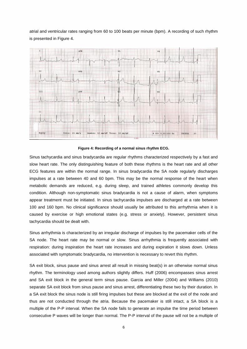
atrial and ventricular rates ranging from 60 to 100 beats per minute (bpm). A recording of such rhythm
is presented in Figure 4.
Figure 4: Recording of a normal sinus rhythm ECG.
Sinus tachycardia and sinus bradycardia are regular rhythms characterized respectively by a fast and
slow heart rate. The only distinguishing feature of both these rhythms is the heart rate and all other
ECG features are within the normal range. In sinus bradycardia the SA node regularly discharges
impulses at a rate between 40 and 60 bpm. This may be the normal response of the heart when
metabolic demands are reduced, e.g. during sleep, and trained athletes commonly develop this
condition. Although non-symptomatic sinus bradycardia is not a cause of alarm, when symptoms
appear treatment must be initiated. In sinus tachycardia impulses are discharged at a rate between
100 and 160 bpm. No clinical significance should usually be attributed to this arrhythmia when it is
caused by exercise or high emotional states (e.g. stress or anxiety). However, persistent sinus
tachycardia should be dealt with.
Sinus arrhythmia is characterized by an irregular discharge of impulses by the pacemaker cells of the
SA node. The heart rate may be normal or slow. Sinus arrhythmia is frequently associated with
respiration: during inspiration the heart rate increases and during expiration it slows down. Unless
associated with symptomatic bradycardia, no intervention is necessary to revert this rhythm.
SA exit block, sinus pause and sinus arrest all result in missing beat(s) in an otherwise normal sinus
rhythm. The terminology used among authors slightly differs. Huff (2006) encompasses sinus arrest
and SA exit block in the general term sinus pause. Garcia and Miller (2004) and Williams (2010)
separate SA exit block from sinus pause and sinus arrest, differentiating these two by their duration. In
a SA exit block the sinus node is still firing impulses but these are blocked at the exit of the node and
thus are not conducted through the atria. Because the pacemaker is still intact, a SA block is a
multiple of the P-P interval. When the SA node fails to generate an impulse the time period between
consecutive P waves will be longer than normal. The P-P interval of the pause will not be a multiple of

7
the baseline P-P interval. Garcia and Miller (2004) define a sinus pause as being three times shorter
than the normal P-P interval and sinus arrest as being greater three times greater than this normal P-P
interval.
2.3.2 Atrial Arrhythmias
A beat or rhythm is said to be ectopic if it originates from a source other than the SA node. Atrial
arrhythmias have their origin in ectopic sites in the atria.
When the underlying regular rhythm is interrupted by an early beat originating from the atria this is
referred to as premature atrial contraction (PAC). Figure 5 shows an ECG with a recording of this
arrhythmic beat. Both the P wave and the QRS complex associated with a PAC appear prematurely
after the last beat. The morphology of the P wave is abnormal and a pause follows the beat. PACs can
be caused by substances such as nicotine and alcohol or due to emotional stress and are usually
asymptomatic. A PAC is said to be nonconducted if the impulse arrives to the AV junction too early,
when it is still in its refractory period, and thus no impulse is conducted through the ventricles. In this
case the abnormally shaped and premature P wave will not be followed by a QRS complex.
Figure 5: ECG showing a premature atrial contraction with an underlying sinus bradycardia rhythm.
Wandering atrial pacemaker refers to the irregular rhythm caused by shifts in the pacemaker site from
the SA node to ectopic sites within the atria. P waves will present different morphologies according to
the origin of the impulse. The rate is usually within normal limits but may also be slower. Wandering
atrial pacemaker is commonly asymptomatic and not clinically significant; it is more frequent among
young patients and athletes.
Atrial tachycardias are ectopic atrial rhythms with fast atrial rates (greater than 100 bpm and going up
to 250 bpm). P waves differ from normal sinus rhythm P waves by their morphology and may be
hidden in the preceding T wave. Atrial rhythm is usually regular whereas ventricular rhythm may either
be regular or irregular depending on whether the AV node is obstructing the passage of some of the
impulses. Atrial tachycardia with block is characterized by an impaired AV conduction. The block may
or may not be variable. Paroxysmal atrial tachycardia starts and stops abruptly and corresponds to at

8
least three consecutive PACs. The rhythm is regular and the heart rate is usually between 140 and
250 bpm. Multifocal atrial tachycardia is an infrequent arrhythmia commonly associated with chronic
pulmonary disease. Impulses are fired by numerous loci which translate into varying P waves. Both
atrial and ventricular rhythms are irregular in this type of atrial tachycardia.
Atrial flutter originates from a single ectopic site that generates impulses usually at a rate around 300
bpm (varying from 250 to 400 bpm). The P waves appear with a saw-toothed shape and are referred
to as flutter waves; they affect the entire baseline. Due to the work of the AV node, the ventricular rate
will not be as high as the atrial rate. This is essential since the lower chambers are not able to tolerate
such high heart rates. The AV conduction ratio will determine the ventricular rate and define the
regularity of the rhythm. Atrial flutter is seldom present in healthy hearts. Control of ventricular rate,
assessing anticoagulation needs and convert the rhythm are the intervention steps to follow.
Atrial fibrillation is the most common type of arrhythmia. The electrical activity on the atria is chaotic,
asynchronous, with rates higher than 400 bpm. Instead of regular contractions, the atria quiver. The P
waves are replaced by irregular wavy deflections, fibrillatory waves, which affect the entire baseline,
as shown in Figure 6. As with atrial flutter, the AV node will block the conduction of the majority of the
impulses thus protecting the ventricles. The irregular conduction of impulses through the AV node
results in a characteristic irregularly irregular ventricular response. Atrial fibrillation can occur
temporarily in healthy individuals, in which case it may revert spontaneously to normal sinus rhythm,
or be associated with heart disease. The same guidelines followed to deal with atrial flutter should be
applied to atrial fibrillation. Controlling the ventricular rate and restoring the sinus rhythm are the
priorities. Some patients may present a chronic atrial fibrillation that will not revert: ventricular rate
control is the only solution in these cases.
Figure 6: Recording of atrial fibrillation.
9
2.3.3 Junctional Arrhythmias and Atrioventricular Blocks
The area around the AV node and the bundle of His is denominated AV junction. Arrhythmias that
originate in this area are referred to as junctional arrhythmias. When pacemaker cells in the AV
junction fire, the impulse spreads backward into the atria (resulting in an inverted P wave) and forward
into the ventricles. Depending on the speed of retrograde and antegrade conductions, the P wave will
either follow or precede the QRS complex. If simultaneous depolarization takes place, the P wave will
be hidden in the QRS complex.
A premature junctional contraction (PJC) is an early beat originating in the AV junction. An abnormally
shaped, premature P wave and a premature QRS complex interrupt an otherwise regular rhythm. The
most common cause of PJCs is digitalis toxicity and if symptoms are present the condition should be
dealt with by correcting the underlying cause. Frequent PJCs may indicate the development of other
junctional rhythms.
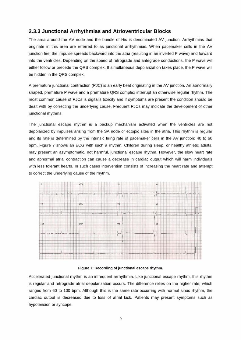
The junctional escape rhythm is a backup mechanism activated when the ventricles are not
depolarized by impulses arising from the SA node or ectopic sites in the atria. This rhythm is regular
and its rate is determined by the intrinsic firing rate of pacemaker cells in the AV junction: 40 to 60
bpm. Figure 7 shows an ECG with such a rhythm. Children during sleep, or healthy athletic adults,
may present an asymptomatic, not harmful, junctional escape rhythm. However, the slow heart rate
and abnormal atrial contraction can cause a decrease in cardiac output which will harm individuals
with less tolerant hearts. In such cases intervention consists of increasing the heart rate and attempt
to correct the underlying cause of the rhythm.
Figure 7: Recording of junctional escape rhythm.
Accelerated junctional rhythm is an infrequent arrhythmia. Like junctional escape rhythm, this rhythm
is regular and retrograde atrial depolarization occurs. The difference relies on the higher rate, which
ranges from 60 to 100 bpm. Although this is the same rate occurring with normal sinus rhythm, the
cardiac output is decreased due to loss of atrial kick. Patients may present symptoms such as
hypotension or syncope.

10
Junctional tachycardia is defined as the occurrence of three or more consecutive PJCs. The rate of
this rhythm is high, above 100 bpm, and the remaining characteristics are the same as junctional
escape rhythm and accelerated junctional escape rhythm. The most common cause of this arrhythmia
is again digitalis toxicity and symptoms of decreased cardiac output may present.
AV blocks refer to the types of arrhythmia in which there is a delay or a fail in the conduction of
electrical impulses through the AV node. This block may be situated in the AV node, the bundle of His
or the bundle branches. AV blocks are classified according to their severity into first-degree, second-
degree (type I and II) and third-degree. In first-degree AV block, the less severe, all the impulses are
conducted through the AV node but this conduction is delayed. This rhythm is regular and atrial and
ventricular rate are the same. The distinguishing feature in an ECG rhythm strip will be the prolonged
but consistent PR interval (superior to 0.20 seconds). This block can progress to a more severe one.
Type I second-degree AV block, or Mobitz type I block, is characterized by a progressive increase of
PR interval until a nonconducted P wave occurs. Although atrial rhythm is regular, the ventricular
rhythm will be irregular and ventricular rate will depend on the number of impulses being conducted
through the AV node. Type II second-degree AV block, or Mobitz type II block, is a rarer but more
serious arrhythmia. In this case the ECG shows no progressive lengthening of the PR interval but
missing QRS complexes will be noted. The ratio of atrial-to-ventricular beats is used to further
characterize this rhythm. Ventricular rate will be regular if this ratio is constant but irregular otherwise.
In third-degree AV block, or complete heart block, all the impulses arriving from the atria are blocked
by the AV node and incapable of reaching the ventricles. In the ECG record, there will be no relation
between P waves and QRS complexes. The atrial rhythm is controlled by the SA node and maintains
a regular rate of 60 to 100 bpm. The ventricular rate will be dictated either by the AV junction or by the
ventricles. In the first case the rate ranges from 40 to 60 bpm and a normal QRS complex can be
observed. In the second case the rate is slower, from 30 to 40 bpm, and the QRS complex will be
wider. Depending on the type of block and the symptoms experienced by the patient, it may be
necessary to insert a temporary or permanent pacemaker.
2.3.4 Ventricular Arrhythmias and Bundle-Branch Blocks
When a bundle-branch block is present ventricular depolarization is said to be sequential: one
ventricle will depolarize before the other. This translates into a wider QRS complex (0.12 seconds or
greater). Right bundle-branch block (RBBB) may appear in a healthy heart but is more commonly
associated with coronary artery disease. RBBB can be temporary, chronic or rate-related (developing
when the heart rate increases). The most common cause of left bundle-branch block (LBBB), shown in
Figure 8, is hypertensive heart disease. LBBB does not occur on healthy individuals and is more
commonly seen among the elderly population.

11
Figure 8: Rhythm strips of a LBBB.
Ventricular arrhythmias originate in the ventricles, below the bundle of His. The electrical impulse will
not follow the normal conduction pathway and an asynchronous depolarization of the ventricles
occurs. The aberrant conduction translates into a wide QRS complex. Ventricular repolarization will
also be affected, which will cause changes in the ST segment and T wave (deflects in opposite
direction to the QRS complex). Logically, since atrial depolarization does not occur, no P wave will be
observable. A fast recognition and treatment of ventricular arrhythmias is necessary since they are
potentially deadly.
Premature ventricular contractions (PVCs) are ectopic beats originating from the ventricles. A
premature, wide, QRS complex is visible in the ECG record. No P wave is associated with the
complex and a compensatory pause follows it. PVCs may occur as a single beat, in clusters of two or
more, or in repeating patterns (bigeminal – see Figure 9, trigeminal or quadrigeminal patterns). PVCs
are common events and can occur in healthy individuals but are more frequent in individuals with
coronary heart disease. Frequent or sustained PVCs can cause a decrease of cardiac output. More
serious arrhythmias can develop from PVCs.
Figure 9: ECG showing a bigeminal rhythm.
12
Ventricular tachycardia is defined as a burst of three or more PVCs fired at a rate exceeding 100 bpm
(normally ranging from 140 to 250 bpm). The ventricular rhythm is usually regular, or slightly irregular,
whereas atrial rhythm and rate cannot be determined. Ventricular tachycardia can last less than 30
seconds, causing few or no symptoms, or be sustained. The latter case should be dealt with
immediately since it is possibly life threatening.
During ventricular fibrillation the ventricles do not contract properly. Instead, the muscle quivers due to
the chaotic electrical activity originating from multiple foci. Irregular fibrillatory waves, differing in shape
and amplitude, appear in the ECG. This rhythm results in no cardiac output and the patient faces
imminent death if it is not reverted (early recognition and defibrillation are key to recovery).
If electrical impulses generated above the bundle of His (either by the sinus node, the atria or the AV
junction) fail to reach the ventricles, or if no impulse is being generated, the last resort pacemaker will
take over. Cells in the ventricles will impose a rhythm to prevent ventricular standstill. A single beat,
referred to as ventricular escape beat, will arise if the rate drops below 40 bpm. The QRS complex will
be wide and the beat will appear late in the conduction cycle. Consecutive ventricular escape beats
form a slow but regular rhythm, the idioventricular rhythm. The ventricular rate ranges from 20 to 40
bpm and it is not possible to determine atrial rate or rhythm. An accelerated idioventricular rhythm has
the same characteristics of an idioventricular rhythm, differing only in terms of heart rate, which ranges
from 50 to 100 bpm. Patients with idioventricular rhythms should be closely monitored because the
progression to a more letal arrhythmia may occur. When symptomatic, the effort should be on
increasing the heart rate, improving cardiac output and reestablishing a normal rhythm. Idioventricular
rhythms should not be suppressed.
During asystole, or ventricular standstill, there is no electrical activity on the ventricles. As a result,
there is no cardiac output and the peripheral pulse and blood pressure are not discernable. The
patient is unconscious and unless the arrhythmia is immediately treated, the situation becomes
irreversible. In an ECG strip, this rhythm appears either as a flat line or as P waves without a QRS
complex. The latter corresponds to the situation when atrial electrical activity is still present.

13
Table 1: Main cardiac rhythms classified according to their origin.
Sinus node rhythms Atrial arrhythmias Junctional arrhythmias and
atrioventricular blocks Ventricular arrhythmias and
bundle-branch blocks
Normal sinus rhythm Wandering atrial pacemaker Premature junctional contraction Bundle-branch block (right or left)
Sinus tachycardia Premature atrial contraction Junctional escape rhythm Premature ventricular contractions
Sinus bradycardia Nonconducted premature atrial contraction
Accelerated junctional rhythm Ventricular tachycardia
Sinus arrhythmia
Atrial tachycardia
Paroxysmal atrial tachycardia
Junctional tachycardia Ventricular fibrillation
Sinus pause
Sinus arrest Atrial tachycardia with block
AV blocks (classified according to severity)
First degree AV block Ventricular escape beat
Sinus exit block Multifocal atrial tachycardia
Second degree AV block, type I (Mobitz I or Wenckebach)
Idioventricular rhythm
Atrial flutter Second degree AV block, type II (Mobitz II)
Accelerated idioventricular rhythm
Atrial fibrillation Third degree AV block (complete heart block)
Ventricular standstill (asystole)
14
2.4 Cardiac Monitors
2.4.1 Standard 12-Lead ECG
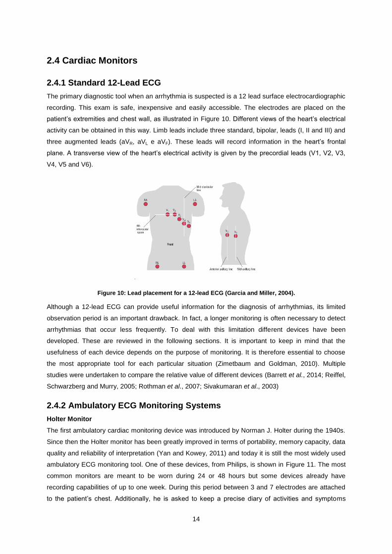
The primary diagnostic tool when an arrhythmia is suspected is a 12 lead surface electrocardiographic
recording. This exam is safe, inexpensive and easily accessible. The electrodes are placed on the
patient’s extremities and chest wall, as illustrated in Figure 10. Different views of the heart’s electrical
activity can be obtained in this way. Limb leads include three standard, bipolar, leads (I, II and III) and
three augmented leads (aVR, aVL e aVF). These leads will record information in the heart’s frontal
plane. A transverse view of the heart’s electrical activity is given by the precordial leads (V1, V2, V3,
V4, V5 and V6).
Figure 10: Lead placement for a 12-lead ECG (Garcia and Miller, 2004).
Although a 12-lead ECG can provide useful information for the diagnosis of arrhythmias, its limited
observation period is an important drawback. In fact, a longer monitoring is often necessary to detect
arrhythmias that occur less frequently. To deal with this limitation different devices have been
developed. These are reviewed in the following sections. It is important to keep in mind that the
usefulness of each device depends on the purpose of monitoring. It is therefore essential to choose
the most appropriate tool for each particular situation (Zimetbaum and Goldman, 2010). Multiple
studies were undertaken to compare the relative value of different devices (Barrett et al., 2014; Reiffel,
Schwarzberg and Murry, 2005; Rothman et al., 2007; Sivakumaran et al., 2003)
2.4.2 Ambulatory ECG Monitoring Systems
Holter Monitor
The first ambulatory cardiac monitoring device was introduced by Norman J. Holter during the 1940s.
Since then the Holter monitor has been greatly improved in terms of portability, memory capacity, data
quality and reliability of interpretation (Yan and Kowey, 2011) and today it is still the most widely used
ambulatory ECG monitoring tool. One of these devices, from Philips, is shown in Figure 11. The most
common monitors are meant to be worn during 24 or 48 hours but some devices already have
recording capabilities of up to one week. During this period between 3 and 7 electrodes are attached
to the patient’s chest. Additionally, he is asked to keep a precise diary of activities and symptoms

15
during the monitoring period to allow for an accurate correlation between symptoms and rhythm
disturbances. Holter monitors generally record the signal from 2 or 3 bipolar leads (commonly chest
modified V5, chest modified V3 and a modified inferior lead) and some systems can derive a 12 lead
ECG from this data (Crawford et al., 1999). Once the recording phase is completed, the monitor is
returned and software is available for the technician to analyze the ECG data. Finally the physician is
provided a report that contains information about average, minimum, and maximum heart rate,
presence and morphology of atrial and ventricular ectopy, nonsustained atrial and ventricular
arrhythmias, AV block, QT interval, and asystole/pauses (Yan and Kowey, 2011). In the presence of
atrial fibrillation (AF) episodes, relevant information such as shortest and longest duration of AF,
burden of AF, heart rate during AF, and pattern of initiation and termination of AF can also be reported
(Mittal, Movsowitz and Steinberg, 2011). The Holter monitor provides a continuous record of ECG but
isn’t prepared to automatically detect arrhythmias and doesn’t have telemetry capabilities. Its short
time of utilization can represent an obstacle in the detection of less frequent arrhythmic episodes.
Figure 11: Philips DigiTrak XT Holter Recorder (Philips, 2014)
Event Recorders
To address the drawbacks of Holter monitors when dealing with infrequent symptoms, the focus has
been on developing other devices that allow cardiac monitoring over a more extended period, namely
event recorders and more recently mobile cardiac outpatient telemetry (MCOT) systems.
Regarding event recorders, a distinction must be made between symptom event monitors and loop
recorders since the latter offer the possibility of registering ECG data prior patient activation whereas
the former do not. Symptom event monitor devices require no leads, they are either carried by the
patient or worn on the wrist, and they can be used for up to 30 days. Small metallic discs are placed
on the back of the device and work as electrodes. Once the patient experiences a symptom or an
irregular beat, he should place the monitor on the chest and activate the recording (or simply press the
activation button if it is a device worn on the wrist). The ECG is recorded from this point onwards but
no information regarding moments preceding the activation is saved. This characteristic may represent
a problem for patients who are unable to quickly activate the device when they experience symptoms,
namely those with syncope (Brignole et al., 2009). The memory capacity of symptom event monitors is
limited and the patient is required to send the recordings to a central monitoring station via telephone.
Loop memory monitors must be worn continuously to allow new ECG data cycles to be acquired and
saved as older, non-informative, cycles are deleted. The duration of the cycles is usually
programmable and can last from several minutes to one hour, depending on the device (Yan and
16
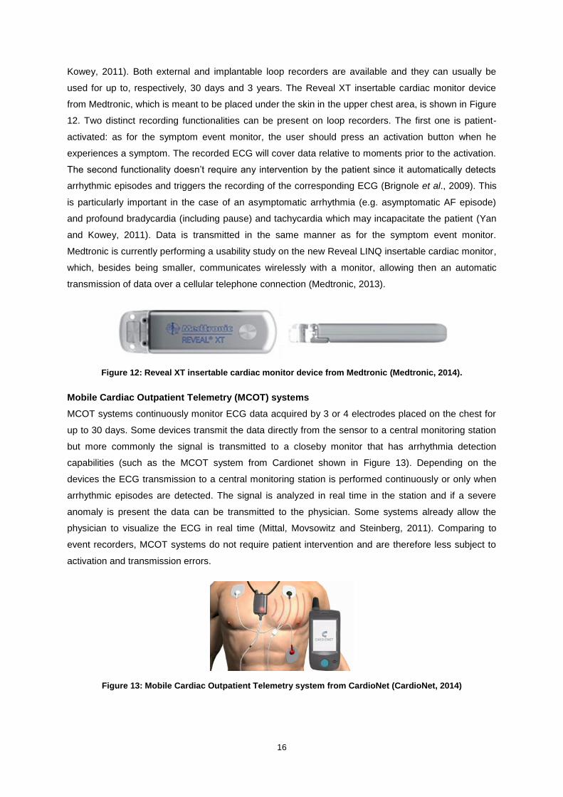
Kowey, 2011). Both external and implantable loop recorders are available and they can usually be
used for up to, respectively, 30 days and 3 years. The Reveal XT insertable cardiac monitor device
from Medtronic, which is meant to be placed under the skin in the upper chest area, is shown in Figure
12. Two distinct recording functionalities can be present on loop recorders. The first one is patient-
activated: as for the symptom event monitor, the user should press an activation button when he
experiences a symptom. The recorded ECG will cover data relative to moments prior to the activation.
The second functionality doesn’t require any intervention by the patient since it automatically detects
arrhythmic episodes and triggers the recording of the corresponding ECG (Brignole et al., 2009). This
is particularly important in the case of an asymptomatic arrhythmia (e.g. asymptomatic AF episode)
and profound bradycardia (including pause) and tachycardia which may incapacitate the patient (Yan
and Kowey, 2011). Data is transmitted in the same manner as for the symptom event monitor.
Medtronic is currently performing a usability study on the new Reveal LINQ insertable cardiac monitor,
which, besides being smaller, communicates wirelessly with a monitor, allowing then an automatic
transmission of data over a cellular telephone connection (Medtronic, 2013).
Figure 12: Reveal XT insertable cardiac monitor device from Medtronic (Medtronic, 2014).
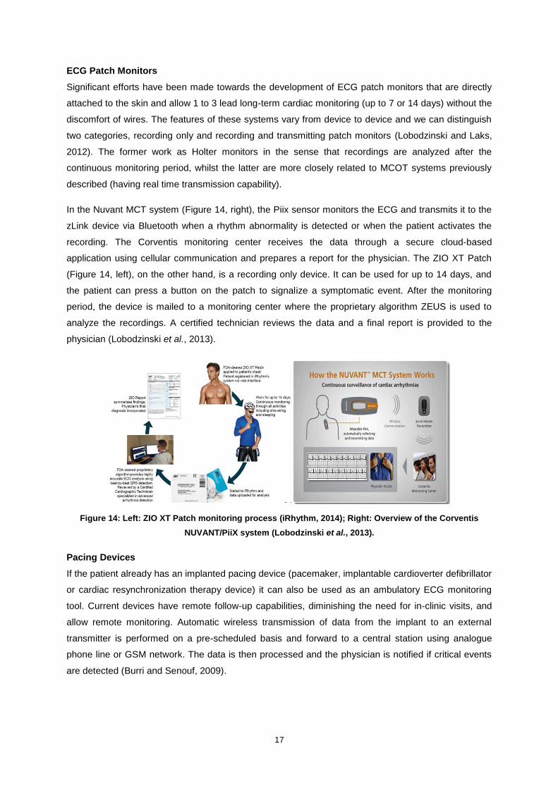
Mobile Cardiac Outpatient Telemetry (MCOT) systems
MCOT systems continuously monitor ECG data acquired by 3 or 4 electrodes placed on the chest for
up to 30 days. Some devices transmit the data directly from the sensor to a central monitoring station
but more commonly the signal is transmitted to a closeby monitor that has arrhythmia detection
capabilities (such as the MCOT system from Cardionet shown in Figure 13). Depending on the
devices the ECG transmission to a central monitoring station is performed continuously or only when
arrhythmic episodes are detected. The signal is analyzed in real time in the station and if a severe
anomaly is present the data can be transmitted to the physician. Some systems already allow the
physician to visualize the ECG in real time (Mittal, Movsowitz and Steinberg, 2011). Comparing to
event recorders, MCOT systems do not require patient intervention and are therefore less subject to
activation and transmission errors.
Figure 13: Mobile Cardiac Outpatient Telemetry system from CardioNet (CardioNet, 2014)
17
ECG Patch Monitors
Significant efforts have been made towards the development of ECG patch monitors that are directly
attached to the skin and allow 1 to 3 lead long-term cardiac monitoring (up to 7 or 14 days) without the
discomfort of wires. The features of these systems vary from device to device and we can distinguish
two categories, recording only and recording and transmitting patch monitors (Lobodzinski and Laks,
2012). The former work as Holter monitors in the sense that recordings are analyzed after the
continuous monitoring period, whilst the latter are more closely related to MCOT systems previously
described (having real time transmission capability).
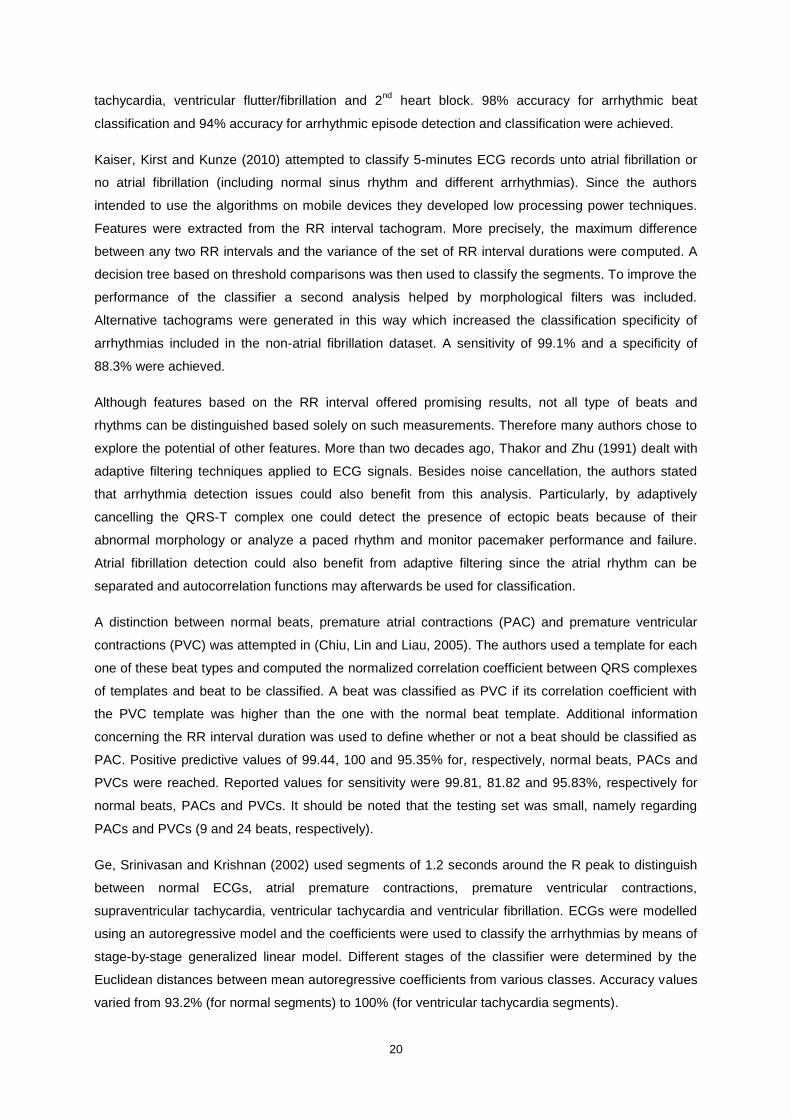
In the Nuvant MCT system (Figure 14, right), the Piix sensor monitors the ECG and transmits it to the
zLink device via Bluetooth when a rhythm abnormality is detected or when the patient activates the
recording. The Corventis monitoring center receives the data through a secure cloud-based
application using cellular communication and prepares a report for the physician. The ZIO XT Patch
(Figure 14, left), on the other hand, is a recording only device. It can be used for up to 14 days, and
the patient can press a button on the patch to signalize a symptomatic event. After the monitoring
period, the device is mailed to a monitoring center where the proprietary algorithm ZEUS is used to
analyze the recordings. A certified technician reviews the data and a final report is provided to the
physician (Lobodzinski et al., 2013).
Figure 14: Left: ZIO XT Patch monitoring process (iRhythm, 2014); Right: Overview of the Corventis
NUVANT/PiiX system (Lobodzinski et al., 2013).
Pacing Devices
If the patient already has an implanted pacing device (pacemaker, implantable cardioverter defibrillator
or cardiac resynchronization therapy device) it can also be used as an ambulatory ECG monitoring
tool. Current devices have remote follow-up capabilities, diminishing the need for in-clinic visits, and
allow remote monitoring. Automatic wireless transmission of data from the implant to an external
transmitter is performed on a pre-scheduled basis and forward to a central station using analogue
phone line or GSM network. The data is then processed and the physician is notified if critical events
are detected (Burri and Senouf, 2009).

18
Other Ambulatory ECG monitoring systems
Other devices are also available ranging from shirts with electrodes to the Alivecor system (Figure 15).
This latter enables ECG lead I acquisition by finger contact with electrodes placed on the back of a
smartphone. The ECG can be visualized in real time or stored and it is immediately transmitted to a
secure server. The stored file can then be interpreted by the physician. Furthermore, an algorithm that
automatically detects atrial fibrillation is implemented on the device (Lau et al., 2013).
Figure 15: Alivecor system (Lau et al., 2013)

19
3. State-of-the-Art
3.1 Review of Beat / Rhythm Classification
In the last few decades a considerable effort was dedicated to develop methods for automatic analysis
of ECG records. A large number of algorithms were developed both to differentiate between different
types of beats and to detect and classify arrhythmias. These vary widely in terms of features extracted
from the ECGs, and classification scheme. When analyzing an ECG, a cardiologist focuses on the
morphology and time domain features to reach a diagnosis. He analyzes durations of waves and
intervals, regularity/irregularity of the rhythm, correspondence between the P waves and the QRS
complexes, amplitudes and polarities, etc. These features have naturally been explored in automatic
ECG analysis but the access to computational resources makes it much easier to extract further
information. Researchers have therefore been able to deal with statistical parameters, frequency
domain features or even more complex information drawn from such theories as the chaos theory.
Regarding the classification scheme, some authors opted for simple methods such as a set of
decision rules whilst others chose to explore more recently developed classifiers such as artificial
neural networks or support vector machines. In this section studies that focused on the automatic beat
or rhythm classification are reviewed. Particular interest is given to the features extracted for
classification and the type of classifier used.
Moody and Mark (1983) compared the performance of multiple classifiers in the detection of atrial
fibrillation. Features were based on RR intervals which are known to be irregular when atrial fibrillation
is present. Markov process models with different averaging techniques (e.g. filter and interpolation)
were tested, as well as a RR predictor array. Improvements were noted with variations from the basic
Markov process but all detectors showed room for improvement.
In an attempt to improve the performances achieved in (Moody and Mark, 1983), Artis, Mark and
Moody (1991) used an artificial neural network to detect atrial fibrillation. The inputs to the network
were the cells of a so-called generalized interval transition matrix. Each RR interval was classified as
short, normal or long and pairs of intervals were assigned to cells of the matrix. A sliding window of
intervals was adopted, allowing a beat-by-beat classification. Atrial fibrillation sensitivity and positive
predictive accuracy were respectively of 92.86 and 92.34%.
More recently other studies continued to use RR-based features for ECG classification tasks. In
(Tsipouras, Fotiadis and Sideris, 2005) both beat and arrhythmia classifications were attempted. First,
using a set of decision rules based on three RR intervals, beats were classified as normal, premature
ventricular contractions, ventricular flutter/fibrillation or 2nd
heart block. The classifications were then
used as input to a deterministic automaton to detect and classify arrhythmic episodes. Six arrhythmias
were considered: ventricular bigeminy, ventricular trigeminy, ventricular couplet, ventricular
20
tachycardia, ventricular flutter/fibrillation and 2nd
heart block. 98% accuracy for arrhythmic beat
classification and 94% accuracy for arrhythmic episode detection and classification were achieved.
Kaiser, Kirst and Kunze (2010) attempted to classify 5-minutes ECG records unto atrial fibrillation or
no atrial fibrillation (including normal sinus rhythm and different arrhythmias). Since the authors
intended to use the algorithms on mobile devices they developed low processing power techniques.
Features were extracted from the RR interval tachogram. More precisely, the maximum difference
between any two RR intervals and the variance of the set of RR interval durations were computed. A
decision tree based on threshold comparisons was then used to classify the segments. To improve the
performance of the classifier a second analysis helped by morphological filters was included.
Alternative tachograms were generated in this way which increased the classification specificity of
arrhythmias included in the non-atrial fibrillation dataset. A sensitivity of 99.1% and a specificity of
88.3% were achieved.
Although features based on the RR interval offered promising results, not all type of beats and
rhythms can be distinguished based solely on such measurements. Therefore many authors chose to
explore the potential of other features. More than two decades ago, Thakor and Zhu (1991) dealt with
adaptive filtering techniques applied to ECG signals. Besides noise cancellation, the authors stated
that arrhythmia detection issues could also benefit from this analysis. Particularly, by adaptively
cancelling the QRS-T complex one could detect the presence of ectopic beats because of their
abnormal morphology or analyze a paced rhythm and monitor pacemaker performance and failure.
Atrial fibrillation detection could also benefit from adaptive filtering since the atrial rhythm can be
separated and autocorrelation functions may afterwards be used for classification.
A distinction between normal beats, premature atrial contractions (PAC) and premature ventricular
contractions (PVC) was attempted in (Chiu, Lin and Liau, 2005). The authors used a template for each
one of these beat types and computed the normalized correlation coefficient between QRS complexes
of templates and beat to be classified. A beat was classified as PVC if its correlation coefficient with
the PVC template was higher than the one with the normal beat template. Additional information
concerning the RR interval duration was used to define whether or not a beat should be classified as
PAC. Positive predictive values of 99.44, 100 and 95.35% for, respectively, normal beats, PACs and
PVCs were reached. Reported values for sensitivity were 99.81, 81.82 and 95.83%, respectively for
normal beats, PACs and PVCs. It should be noted that the testing set was small, namely regarding
PACs and PVCs (9 and 24 beats, respectively).
Ge, Srinivasan and Krishnan (2002) used segments of 1.2 seconds around the R peak to distinguish
between normal ECGs, atrial premature contractions, premature ventricular contractions,
supraventricular tachycardia, ventricular tachycardia and ventricular fibrillation. ECGs were modelled
using an autoregressive model and the coefficients were used to classify the arrhythmias by means of
stage-by-stage generalized linear model. Different stages of the classifier were determined by the
Euclidean distances between mean autoregressive coefficients from various classes. Accuracy values
varied from 93.2% (for normal segments) to 100% (for ventricular tachycardia segments).

21
Numerous authors chose to construct a feature set containing both temporal and morphological
information.
In (Iliev, Krasteva and Tabakov, 2007) a set of decision rules was established to classify beats as
either normal or ventricular ectopic beats. Morphological and time-domain features were extracted. A
QRS pattern matrix was constructed (holding information about amplitude-temporal distribution of
QRS) and deviation of RR interval from the mean RR interval was also considered. Sensitivity and
specificity values were reported to be respectively 99.81 and 98.87% in a noise-free test set.
De Chazal, O’Dwyer and Reilly (2004) compared the performance of 12 classifier configurations in
distinguishing 5 different beat types. Three categories of features were used: RR interval features,
heartbeat interval features and ECG morphology features. Classifier configurations were based on
linear discriminants (LDs), a statistical classifier model. The best results were obtained when two
leads were used for classification (two LD classifiers employed) and the results were posteriorly
combined. For supraventricular ectopic beats sensitivity and positive predictive values of 75.9 and
38.5% were obtained. Regarding ventricular ectopic beats, the sensitivity was 77.7% and the positive
predictivity was 81.9%.
In (Melgani and Bazi, 2008) multiple tests were performed to compare the performance of different
classifiers on distinguishing between normal beats, atrial premature beats, ventricular premature
beats, right bundle branch block, left bundle branch block and paced beats. Focus was given to
support vector machines and a new improved method consisting on the combination of particle swarm
optimization with this classifier to improve its generalization performance. The two other classifiers
used as reference were the k-nearest neighbor and the neural network and some tests included a
feature selection step with principal component analysis Two types of features were extracted:
morphological and temporal (QRS complex duration, RR interval and average RR interval over the 10
last beats). The authors reported an overall accuracy of 89.72% with the proposed method which was
higher than the values obtained with other classifiers.
The potential of neural networks was explored from early on and continues to be one of the main
machine learning classifiers used in ECG beat/rhythm analysis.
In (Hu et al., 1993) an artificial neural network was used to distinguish between normal and abnormal
beat patterns, as well as to classify 12 different abnormal beat morphologies. Inputs to the network
consisted of an amplitude-scaled QRS beat pattern. When using a composite classifier where the first
network distinguished between normal and abnormal morphologies and the second one classified the
abnormal beats, a classification rate of 84.5% was obtained. Accuracy varied greatly between beat
types.
Clayton, Murray and Campbell (1994) attempted to use neural networks to distinguish between
ventricular fibrillation (VF) and VF-like events. Inputs to the network consisted of 5 frequency domain
parameters derived from the Fourier spectrum of the signal and the mean threshold crossing interval.
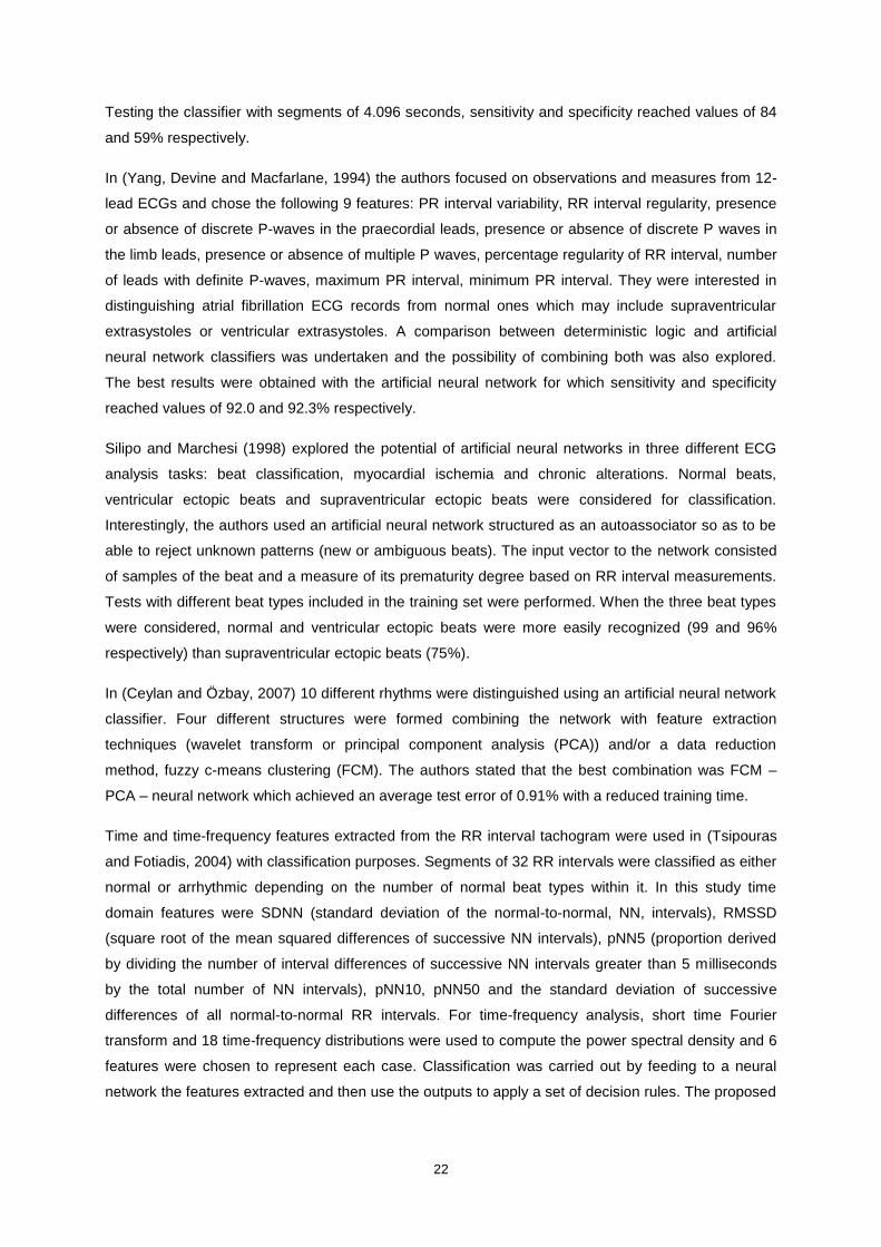
22
Testing the classifier with segments of 4.096 seconds, sensitivity and specificity reached values of 84
and 59% respectively.
In (Yang, Devine and Macfarlane, 1994) the authors focused on observations and measures from 12-
lead ECGs and chose the following 9 features: PR interval variability, RR interval regularity, presence
or absence of discrete P-waves in the praecordial leads, presence or absence of discrete P waves in
the limb leads, presence or absence of multiple P waves, percentage regularity of RR interval, number
of leads with definite P-waves, maximum PR interval, minimum PR interval. They were interested in
distinguishing atrial fibrillation ECG records from normal ones which may include supraventricular
extrasystoles or ventricular extrasystoles. A comparison between deterministic logic and artificial
neural network classifiers was undertaken and the possibility of combining both was also explored.
The best results were obtained with the artificial neural network for which sensitivity and specificity
reached values of 92.0 and 92.3% respectively.
Silipo and Marchesi (1998) explored the potential of artificial neural networks in three different ECG
analysis tasks: beat classification, myocardial ischemia and chronic alterations. Normal beats,
ventricular ectopic beats and supraventricular ectopic beats were considered for classification.
Interestingly, the authors used an artificial neural network structured as an autoassociator so as to be
able to reject unknown patterns (new or ambiguous beats). The input vector to the network consisted
of samples of the beat and a measure of its prematurity degree based on RR interval measurements.
Tests with different beat types included in the training set were performed. When the three beat types
were considered, normal and ventricular ectopic beats were more easily recognized (99 and 96%
respectively) than supraventricular ectopic beats (75%).
In (Ceylan and Özbay, 2007) 10 different rhythms were distinguished using an artificial neural network
classifier. Four different structures were formed combining the network with feature extraction
techniques (wavelet transform or principal component analysis (PCA)) and/or a data reduction
method, fuzzy c-means clustering (FCM). The authors stated that the best combination was FCM –
PCA – neural network which achieved an average test error of 0.91% with a reduced training time.
Time and time-frequency features extracted from the RR interval tachogram were used in (Tsipouras
and Fotiadis, 2004) with classification purposes. Segments of 32 RR intervals were classified as either
normal or arrhythmic depending on the number of normal beat types within it. In this study time
domain features were SDNN (standard deviation of the normal-to-normal, NN, intervals), RMSSD
(square root of the mean squared differences of successive NN intervals), pNN5 (proportion derived
by dividing the number of interval differences of successive NN intervals greater than 5 milliseconds
by the total number of NN intervals), pNN10, pNN50 and the standard deviation of successive
differences of all normal-to-normal RR intervals. For time-frequency analysis, short time Fourier
transform and 18 time-frequency distributions were used to compute the power spectral density and 6
features were chosen to represent each case. Classification was carried out by feeding to a neural
network the features extracted and then use the outputs to apply a set of decision rules. The proposed

23
algorithms reached sensitivity and specificity values of 87.5 and 89.5%, respectively, for time domain
analysis and 90 and 93%, respectively, for time-frequency domain analysis.
If artificial neural networks have drawn considerable attention as classifiers, wavelet transforms have
earned their place in the feature extraction process. Compared to other frequency analysis methods,
e.g. Fourier transform, wavelet analysis allows a multi-scale decomposition and overcomes some
drawbacks in terms of frequency resolution.
Classification of normal sinus rhythm, atrial fibrillation, ventricular fibrillation and ventricular
tachycardia ECG records was addressed in (Khadra, Al-Fahoum and Al-Nashash, 1997). The wavelet
transform of the signal was computed and energy parameters were retrieved from the scalogram
(squared magnitude of the wavelet transform). Different time-frequency bands were defined and the
energy of the signal within each region was computed. Signals were classified as one of the 4 rhythms
according to a set of rules. A relatively small number of ECG records was used and sensitivity and
specificity values lied between 83.3 and 92.3%.
In (Al-Fahoum and Howitt, 1999) an attempt was made to distinguish between the same four rhythms.
Wavelet transforms (WTs) were used to extract features and a radial basis function neural network
was adopted as classifier. A beat-by-beat classification was performed. The feature vector consisted
of 3 relative energy terms used to characterize the QRS complex at different WT scales and relative
energy in the signal before the QRS, in the QRS and after the QRS. An overall correct classification of
97.5% was achieved though sensitivity and specificity values varied widely between classes. Whereas
100% correct classification of ventricular fibrillation and ventricular tachycardia signals was obtained,
the sensitivity and specificity of atrial fibrillation segments was respectively 95.2 and 85.7%.
Güler and Übeyli (2005) attempted to perform a beat-by-beat classification to distinguish between
normal, congestive heart failure, ventricular tachyarrhythmia and atrial fibrillation beats. Statistical
features were extracted from the wavelet coefficients to try to represent both the frequency distribution
of the signal and changes in frequency distribution. These were: mean of the absolute values of the
coefficients in each sub-band, average power of the wavelet coefficients in each sub-band, standard
deviation of the coefficients in each sub-band and ratio of the absolute mean values of adjacent sub-
bands. A combined neural network model, where the outputs of the first set of networks were fed to a
second level network, was employed. An overall classification accuracy of 96.94% was achieved.
Kara and Okandan (2007) developed a method to distinguish between normal sinus rhythm and atrial
fibrillation ECG segments. Wavelet theory was used to decompose the 60 seconds signals until the
sixth level and power spectral density of each one of the 6 details and one approximation signals were
computed. Average power spectral density values over 6 frequency sub-bands were then obtained
which amounted to a total of 42 features per ECG segment. Of these features, 22 were used as input
to an artificial neural network. The authors reported an accuracy of 100% in a test set composed by 24
normal ECGs and 28 atrial fibrillation segments.

24
Martis et al. (2012) compared the performance of a neural network (NN), a support vector machine
(SVM) and a Gaussian mixture model (GMM) in the distinction between normal beats and 12 different
beat types. Features were extracted from the wavelet decomposition of the signal. A feature selection
method, principal component analysis, was applied to the sub-bands that covered the frequencies of
interest. This reduced set of coefficients was then fed to the classifiers. Overall accuracy values of
87.36, 93.41 and 95.60% were obtained for GMM, NN and SVM classifiers respectively.
Other studies have tested the possibility of constructing a feature set not based solely on parameters
extracted from the wavelet transform. In (Prasad and Sahambi, 2003), information about RR intervals
was used in combination with 23 selected wavelet transform coefficients to distinguish between
normal and 12 abnormal beat types. An artificial neural network was used as classifier and an overall
accuracy of 96.77% was reached. More recently beat classification was achieved after an adaptive
feature extraction method was applied to a large set of features (Shen et al., 2012). These included
wavelet coefficients, statistical properties of the coefficients and electrophysiological measures (RR
interval information, amplitude of waves, ratio between different intervals,etc.). The classification
scheme included the use of k-means clustering, one-against-one support vector machine and a
modified majority voting mechanism. A recognition rate of 98.92% was reported by the authors but
accuracy varied between beat types.
Classification of normal, premature ventricular contraction and other beat types was attempted in
(Inan, Giovangrandi and Kovacs, 2006). The feature set combined a set of coefficients from the
wavelet transform and timing information. A neural network classifier was employed. Timing
information consisted of a RR interval ratio which translates the deviation from a constant beat rate.
Multiple tests were performed regarding both the decomposition level and the feature vector length.
The best results led to an accuracy of 95.2%.
In (Sambhu and Umesh, 2013) a beat classification scheme was proposed to distinguish between
normal beats, left and right bundle branch block, atrial and ventricular premature contractions, paced
and fusion beats. A combination of temporal, morphological and statistical features was used for
classification. Some of these features were extracted after wavelet decomposition of the signal. Prior
to classification, a feature selection method was employed. Multiple one-against-one support vector
machines were employed and the final classification was given by a maximum voting mechanism. The
authors reported an overall accuracy superior to 98%.
In (Ye, Kumar and Coimbra, 2012), 16 different beat types were considered for classification.
Morphological features were extracted by two different methods: wavelet decomposition of the signal
and independent component analysis. Feature reduction of this set of features was achieved resorting
to principal component analysis. Four dynamic features were also considered: previous RR, post RR,
local RR and average RR. The signal recorded by each one of the two leads was independently
classified by a support vector machine and a final decision was taken by fusing the two results. Overall
accuracies of 99.3 and 86.4% were obtained respectively for the “class-oriented” and “subject-
oriented” approaches.

25
In the last few years some studies were published were new approaches regarding the features for
classification were explored. In (Wang et al., 2001) a new approach that deals with the nonlinear and
non-stationary characteristics of the ECG from the viewpoint of multifractality was presented. Atrial
fibrillation, ventricular tachycardia and ventricular fibrillation ECG records were considered for
classification. Short-time generalized dimensions were computed and input to a new fuzzy Kohonen
network. Accuracy values of 97.8, 97.2 and 99.4% were reported respectively for ventricular
tachycardia, ventricular fibrillation and atrial fibrillation. Specificity values were higher for atrial
fibrillation and ventricular tachycardia records.
Owis et al. (2002) focused on the nonlinear dynamics of ECG signals to detect and classify
arrhythmias. Two features from the field of chaotic dynamical system theory were chosen to represent
3 seconds ECG signals: the correlation dimension and the largest Lyapunov exponent. An attempt
was made to distinguish between normal and abnormal ECG signals and to classify the different types
of arrhythmias. These included ventricular couplet, ventricular tachycardia, ventricular bigeminy and
ventricular fibrillation. The performance in such tasks of the minimum distance classifier, the k-NN
classifier and Bayes minimum error classifier was accessed. The statistical analysis carried out
showed the potential of the two features in the detection of ECG abnormalities but the ability to
distinguish between types of arrhythmias was limited. Specificity and sensitivity values varied among
classifiers.
Bakhshi et al. (2010) developed a linear classifier based on instantaneous frequency (IF) to distinguish
between normal signals and diseased ones. The IF was estimated using the discrete power spectral
density calculated by means of the Fourier transform of the ECG signal. Sensitivity and specificity
values were reported to be respectively of 97.82 and 100% for 5 minutes portions of ECG records.
In (Anas, Lee and Hasan, 2010) the authors focused on ventricular tachycardia (VT) and ventricular
fibrillation (VF) ECG records with the purpose of identifying such arrhythmias. A sequential detection
algorithm was developed and the first step consisted of separating VT/VF signals from the remaining
ones. This was achieved by computing the mean absolute value of a signal and comparing it to a
predefined threshold value. An accuracy of 99.07% with a specificity value of 99.39% was obtained. In
a second step an attempt was made to distinguish between VT and VF. In order to do so the authors
used empirical mode decomposition to extract the intrinsic mode functions from the signals. The
difference between the original signal and the sum of its first two intrinsic mode functions was then
computed. The mean absolute value of this difference signal was used to classify VT and VF signals.
The authors further went on to distinguish between shockable and non-shockable rhythms by
determining the heart rate. An overall accuracy of 99.21% was reported.
Sufi, Khalil and Mahmood (2011) adopted an original approach for ECG diagnosis: the feature
extraction process was carried out directly on the compressed ECG. By circumventing the
decompression phase, compressed and encrypted ECG packets sent by a mobile phone to a
monitoring service could be promptly analyzed and further delays avoided. A set of 157 attributes,
corresponding to the frequency of each character/numeric sub groups, was extracted and a correlation

26
based feature subset selection technique was then applied. A statistical clustering technique,
expectation maximization algorithm, was used to distinguish between normal and abnormal ECGs. A
100% accuracy rate was reported in a small test set of 20 segments.
In this work two types of features are used: spectral features extracted using the wavelet transform
and an estimation of the power spectral density; and time domain parameters translating heart rate
characteristics. The performance of three classifiers is compared: k-nearest neighbor, multilayer
perceptron and support vector machine. Before detailing the methodology followed, the theoretic
concepts necessary are reviewed.
3.2 Wavelet Transform
Wavelet analysis is a powerful tool to obtain a time-frequency representation of a signal. Contrary to
short time Fourier transform (STFT) the wavelet transform is a multi-resolution analysis and therefore
overcomes the difficulty of finding an optimal resolution for analyzing the signal. It allows us to
examine the low frequency content (spread over a larger amount of time) without compromising the
accurate time domain localization of high frequency features. After the choice of an analyzing wavelet
function, ψ(t), the wavelet transform of a continuous time signal x(t) is defined as:
𝑊𝑎𝑥(𝑏) =1
√𝑎∫ 𝑥(𝑡)𝜓∗ (
𝑡 − 𝑏
𝑎) 𝑑𝑡
+∞
−∞
(1)
where 𝑎 and 𝑏 are respectively the dilation and location parameter of the wavelet and 𝜓∗(𝑡) is the
complex conjugate of the analyzing wavelet function. For it to be considered as analyzing wavelet, the
function should satisfy a number of mathematical properties. These are reviewed in (Addison, 2005);
in particular, the function must have finite energy and respect the admissibility condition which implies
a zero average. The analyzing wavelet function is also referred to as mother wavelet since a family of
functions is defined from this prototype by applying translations and dilations. The wavelet transform
can therefore be seen as the decomposition of the signal by this set of basis functions.
A discretized version of the continuous wavelet transform described above is often used and a dyadic
grid, with 𝑎 = 2𝑚 and 𝑏 = 2𝑚𝑛, is commonly employed. The basis functions can then be written as:
𝜓𝑚,𝑛(𝑡) = 2−𝑚 2⁄ 𝜓(2−𝑚𝑡 − 𝑛) (2)
A fast implementation of the decomposition algorithm can be achieved by recursively applying high-
pass and low-pass filters to the wavelet coefficients from the previous scale. This filter bank algorithm,
presented by Mallat (1989), is illustrated in Figure 16. The filter coefficients of the high-pass, H, and
low-pass, G, decomposition filters characterize the wavelet used.

27
Figure 16: Mallat’s algorithm for discrete wavelet decomposition (Martínez et al., 2004).
The redundant discrete wavelet transform (RDWT), or algorithme à trous, can also be used to
decompose the signal. This discretized version of the continuous wavelet transform is shift invariant,
having the same spatial sampling rate in all scales. The downsampling operations represented in
Figure 16 are discarded, and the filter responses are upsampled. Additional information concerning
the RDWT and its implementation can be found in (Fowler, 2005).
In the last couple of decades, applications of wavelet theory to ECG analysis have been largely
explored (Addison, 2005). These include signal denoising, detection and delineation of ECG
characteristic points, heart rate variability analysis, ECG data compression and feature extraction for
beat/rhythm classification. The choice of mother wavelet is an important step in all these applications
and multiple functions have been tested including Daubechies, Morlet, spline, raised cosine and
quadratic spline wavelets.
3.3 Power Spectral Density
The power spectral density (PSD) represents the distribution of the signal power over different
frequencies. Welch’s method is commonly employed to compute the PSD (Welch, 1967). The signal
𝑥(𝑗), 𝑗 = 0, … , 𝑁 − 1 is first split into 𝐾 possibly overlapped segments of length 𝐿 as illustrated by
Figure 17. A window 𝑤(𝑗), 𝑗 = 0, … , 𝑁 − 1 is applied to each segment and the finite Fourier transform of
these sequences are then computed as given by equation (3).
Figure 17: Schematic representation of the splitting of the signal.
𝐴𝑘(𝑛) =1
𝐿∑ 𝑥𝑘(𝑗)𝑤(𝑗)𝑒−
2𝑘𝑖𝑗𝑛𝐿
𝐿−1
𝑗=0
(3)

28
The so-called modified periodograms are obtained after squaring the magnitude of the result:
𝐼𝑘(𝑓𝑛) =𝐿
𝑈|𝐴𝑘(𝑛)|2 𝑘 = 1,2, … , 𝐾 (4)
where 𝑓𝑛 and 𝑈 are respectively given by:
𝑓𝑛 =𝑛
𝐿 𝑛 = 0, … , 𝐿/2 (5)
𝑈 =1
𝐿∑ 𝑤2(𝑗)
𝐿−1
𝑗=0
(6)
Finally, the spectral estimate �̂� is the average of the individual periodograms:
�̂�(𝑓𝑛) =1
𝐾∑ 𝐼𝑘(𝑓𝑛)
𝐾
𝑘=1
(7)
3.4 Classifiers
3.4.1 k-Nearest Neighbors
The concept behind the k-nearest neighbors (kNN) classifier is a very simple one. Assuming we have
a dataset for which we know the true labels of the samples, new samples can be classified according
to their similarity with labeled samples. A set of features is chosen to represent each sample and the
similarity between samples is measured resorting to a metric. If desired, different weights can be
attributed to the neighbors, assuring for instance that closest neighbors contribute in a larger extent to
the fit. The ‘training set’ is used to construct a neighbor base and the test patterns are classified
according to the class of the k most similar neighbors. An example of binary classification using two
features is shown in Figure 18. A more detailed explanation of this classifier can be found in (Duda,
Hart and Stork, 2001).
Figure 18: Example of kNN binary classification problem. Two features are used to distinguish between class 1, blue circles, and class 2, red triangles. When 3 neighbors are used for classification the test
sample (green square) is assigned to class 2.
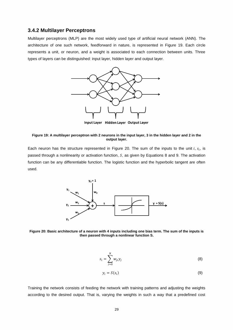
29
3.4.2 Multilayer Perceptrons
Multilayer perceptrons (MLP) are the most widely used type of artificial neural network (ANN). The
architecture of one such network, feedforward in nature, is represented in Figure 19. Each circle
represents a unit, or neuron, and a weight is associated to each connection between units. Three
types of layers can be distinguished: input layer, hidden layer and output layer.
Figure 19: A multilayer perceptron with 2 neurons in the input layer, 3 in the hidden layer and 2 in the output layer.
Each neuron has the structure represented in Figure 20. The sum of the inputs to the unit 𝑖, 𝑠𝑖, is
passed through a nonlinearity or activation function, 𝑆, as given by Equations 8 and 9. The activation
function can be any differentiable function. The logistic function and the hyperbolic tangent are often
used.
Figure 20: Basic architecture of a neuron with 4 inputs including one bias term. The sum of the inputs is then passed through a nonlinear function S.
𝑠𝑖 = ∑ 𝑤𝑗𝑖𝑦𝑗
𝑁
𝑗=0
(8)
𝑦𝑖 = 𝑆(𝑠𝑖) (9)
Training the network consists of feeding the network with training patterns and adjusting the weights
according to the desired output. That is, varying the weights in such a way that a predefined cost

30
function is minimized. This cost function can simply be a measure of the error between output and
desired output. For each training pattern 𝑘, with 𝑘 = 1, … , 𝐾, if 𝒐𝑘 and 𝒅𝑘 are, respectively, outputs and
desired outputs, the error vector will be given by:
𝒆𝑘 = 𝒐𝑘 − 𝒅𝑘 (10)
For each training pattern a scalar measure of the error can be given by Equation (11) and, in the
whole training set, the deviation of the network from its ideal behavior is given by Equation (12).
𝐸𝑘 = ‖𝒆𝑘‖2 (11)
𝐸 = ∑ 𝐸𝑘
𝐾
𝑘=1
(12)
The gradient descent method can then be used to update the weights:
𝒘𝑛+1 = 𝒘𝑛 − 𝜂∇𝐸 (13)
where 𝜂 is the step size parameter, or learning rate. The main difficulty of this method is the
computation of the gradient components. In practice this is achieved by using the backpropagation
method. A new network, the error propagation network, is constructed from the initial network by
linearizing nonlinear elements and reversing it. Each training pattern is input to the original network
and the partial derivative of the error with respect to the output is then input to the error propagation
network. The partial derivative relative to a weight is then simply given by the product of the inputs of
the branches corresponding to that weight in the original network and in the backpropagation network.
The training phase ends when a stopping criterion is reached (usually either when the error is below a
predefined threshold or when the maximum number of epochs is reached). More details about the
backpropagation algorithm, including examples, can be found in (Beale and Fiesler, 1997).
Training the network may become a very lengthy process. To deal with this limitation acceleration
techniques are often adopted (e.g. adaptive step sizes or momentum). The weight update considering
the momentum technique is given by the following equations:
𝒘𝑛+1 = 𝒘𝑛 + ∆𝒘𝑛 (14)
∆𝒘𝑛 = −𝜂∇𝐸 + 𝛼∆𝒘𝑛−1 (15)
where 𝛼 is the momentum term, 0 ≤ 𝛼 < 1. These equations can be interpreted as follows. At valleys
where the gradient is relatively constant in terms of direction, the 𝛼 term contributes to an increase of
the contribution of this gradient at each iteration. This results in an increased speed of convergence.
On the other hand, at points where the gradient oscillates a lot, this term cancels relatively well the
gradient term depending on 𝜂, thus dampening oscillations.

31
3.4.3 Support Vector Machines
SVMs, like ANNs and kNN, are a type of supervised learning classifiers. Considering the example
illustrated in Figure 21, the goal of the training process is to define the parameters that describe the
boundary between the two different classes (boundary represented by a continuous line). This
boundary should be the one that lies as far as possible from the closest training patterns. Once a new
sample is presented it will be classified according to the side of the boundary it falls upon. Dashed
lines represent the margins and the samples highlighted in green are referred to as support vectors.
As can be seen these are the samples that lie the closest to the boundary. Although a two-
dimensional problem is pictured here (only two features for each pattern), the idea is exactly the same
for N-dimensional linearly separable data. In such case the boundary and margins will be hyperplanes.
Figure 21: Example of a SVM binary classification problem. Highlighted in green are the three support vectors. Continuous and dashed lines represent respectively decision boundary and margins.
To describe the problem from a mathematical point of view let us consider that M training patterns of
dimension N are available: 𝒙𝑖 𝑤ℎ𝑒𝑟𝑒 𝑖 = 1 … 𝑀, 𝒙 ∈ ℛ𝑁 . We shall denote the class of the training
pattern 𝑖 by 𝑦𝑖. Each pattern belongs to one of the following two classes: 𝑦𝑖 = +1 or 𝑦𝑖 = −1. If 𝒘 is
normal to the hyperplane and 𝑏
‖𝒘‖ is the distance from the hyperplane to the origin, the hyperplane is
described by 𝒙 ∙ 𝒘 + 𝑏 = 0. The training patterns will then satisfy equations (16) and (17) which can
be combined to (17).
𝒙𝑖 ∙ 𝒘 + 𝑏 ≥ +1 for 𝑦𝑖 = +1 (16)
𝒙𝑖 ∙ 𝒘 + 𝑏 ≤ −1 for 𝑦𝑖 = −1 (17)
𝑦𝑖(𝒙𝑖 ∙ 𝒘 + 𝑏) − 1 ≥ 0 ∀𝑖 (18)
In order to maximize the margins, which are simply the distance between support vectors and the
boundary, we must find the parameters 𝒘 and 𝑏 that respect:
min ‖𝒘‖ such that 𝑦𝑖(𝒙𝑖 ∙ 𝒘 + 𝑏) − 1 ≥ 0 ∀𝑖 (19)

32
Since minimizing ‖𝒘‖ is equivalent to minimizing 1
2‖𝒘‖2, this term can be substituted in the equation
above. The problem is then reduced to a convex quadratic optimization problem and Lagrange
multipliers are used to take into account the constraint (Fletcher, 2009).
The example considered here is a very simple one where the classes are fully linearly separable. In
practice this is not the case and it becomes necessary to adjust equations (16) and (17) to allow
misclassifications. This is done considering a new slack variable 𝜉𝑖 for each training pattern 𝑖 with
𝜉𝑖 ≥ 0 for all patterns. For each pattern the associated variable measures its degree of
misclassification. Equations (20) and (21) are obtained and can be combined into equation (22). This
formulation is commonly referred to as soft margin SVM.
𝒙𝑖 ∙ 𝒘 + 𝑏 ≥ +1 − 𝜉𝑖 for 𝑦𝑖 = +1 (20)
𝒙𝑖 ∙ 𝒘 + 𝑏 ≤ −1 + 𝜉𝑖 for 𝑦𝑖 = −1 (21)
𝑦𝑖(𝒙𝑖 ∙ 𝒘 + 𝑏) − 1 + 𝜉𝑖 ≥ 0 ∀𝑖 (22)
The new function to minimize is given by equation (23). A balance between maximizing the margins
and reducing the number of misclassifications is sought. To control the trade-off between these two
goals a penalty parameter 𝐶 is introduced. By increasing 𝐶 we ensure that more training patterns will
be correctly classified, at the expense of a more complex, unsmooth, boundary surface. If a very high
value is chosen for 𝐶 then the classifier may lose its generalization capability.
min1
2‖𝒘‖2 + 𝐶 ∑ 𝜉𝑖
𝐿
𝑖=1
s. t. 𝑦𝑖(𝒙𝑖 ∙ 𝒘 + 𝑏) − 1 + 𝜉𝑖 ≥ 0 ∀𝑖 (23)
Until now it was assumed that the classes are linearly separable. However this is seldom the case and
it becomes necessary to recur to a more complex procedure. The idea is to map the original features
into a different feature space (commonly with a higher dimensionality) where they become linearly
separable. In practice this mapping is done implicitly by using the well-known kernel trick (Fletcher,
2009).
SVMs were originally developed to solve binary classification problems. However, it is much more
common to deal with multiclass problems. Multiple approaches have been proposed to adapt the SVM
formulation for these types of problems. The one-against-one and the one against-all SVMs are the
two most popular formulations. Here, the one-against-one approach was used, which has been shown
to be a suitable choice (Hsu and Lin, 2002). For each pair of classes, a binary classifier is constructed,
amounting to a total of 𝑘(𝑘 − 1)/2 classifiers, where 𝑘 is the total number of classes. Each classifier is
trained using data from the two corresponding classes. Once a new pattern is presented all classifiers
are ‘activated’ to assign it a label. The selected class label is the one that occurs the most.

33
4. Methodology The methodology proposed in this thesis is schematized in Figure 22, encompassing the following
steps: signal acquisition and processing (including filtering and segmentation steps) and finally rhythm
classification.
Figure 22: Automatic signal analysis methodology.
The classification phase is further detailed in Figure 23 where the main steps are feature extraction,
feature normalization, classifier training and testing.
Figure 23: Steps of the classification task.
In the following subsections all the steps mentioned above will be detailed.
4.1 Signal Acquisition and Processing
4.1.1 BITalino system
The BITalino is a low-cost biosignal acquisition system (Guerreiro et al., 2013). It includes sensors for
multiple physiological signals: electromyography, electrodermal activity and ECG. It further provides
an accelerometer, a light sensor and a light-emitting diode. Software for real time acquisition and
visualization is also available (Alves et al., 2013).
Figure 24: BITalino system used for ECG acquisitions.

34
Since a pervasive acquisition setup is sought, this system was used to acquire ECG records at the
fingers. A sampling rate of 1000 Hz was used. It has been shown that the ECG acquired with the
BITalino system at the fingers is highly correlated with lead I from traditional 12 leads systems
(Carreiras et al., 2013). It is therefore reasonable to expect that cardiac conditions that can be
diagnosed by analyzing the lead I of the ECG can also be detected with this pervasive acquisition
system.
4.1.2 Filtering
The filter process adopted here has been previously used with ECG data acquired with the BITalino
system, mainly for biometric applications. First, two median filters are applied to remove the baseline,
with window sizes of 0.2 and 0.3 seconds. A finite impulse response low-pass filter with cutoff
frequency of 40 Hz is then used to deal with high frequency noise. Due to the characteristics of the
acquisition system, muscular activity is frequently picked up, thus a final moving average filter, with a
window of 28 milliseconds, is applied.
Figure 25: 10 seconds extract of an ECG acquired with the BITalino. Raw (left) and filtered (right) records are shown.
4.1.3 R peak detection
An algorithm based on the work of (Hamilton, 2002) was used to detect R peaks. As shown in Figure
26, the detection method starts with a filter step. First, low-pass and high-pass filters are applied to the
signal, with cutoff frequencies respectively of 16 and 8 Hz. The derivative is then calculated and its
absolute value is computed. Finally, a moving average with a window of 80 milliseconds is computed.

35
Figure 26: Schematic representation of the R peak detection algorithm. Adapted from (Hamilton, 2002).
Once the peaks are detected, they ought to be classified either as a QRS complex or noise. This
decision relies upon a set of detection rules that take into consideration peak height, peak location
(relative to the last QRS peak) and maximum derivative. The accuracy of the algorithm depends on
the computation of a detection threshold, defined using QRS peaks and noise peaks heights, as
shown in Equation 24.
Detection Threshold = Average Noise Peak + TH × (Average QRS Peak − Average Noise Peak) (24)
where TH is the threshold coefficient, which represents a compromise between correct and false
detections. Decreasing the TH will lead to a higher number of correct detections, at the expense of
false detections.
The following detection rules are applied:
1. All peaks that precede or follow larger peaks by less than 200 milliseconds are ignored.
2. If a peak occurs, the presence of both positive and negative slopes in the raw signal is
checked. If these are not present, the peak represents a baseline shift.
3. If the peak occurred within 360 milliseconds of a previous detection, the value of the maximum
derivative in the raw signal is checked. If it is smaller than half the maximum derivative of the
previous detection, the peak is assumed to be a T-wave.
4. If the peak is larger than the detection threshold, it is considered a QRS complex, otherwise it
should be considered noise.

36
5. If no QRS has been detected within 1.5 RR intervals, there was a peak that was larger than
half the detection threshold, and the peak followed the preceding detection by at least 360
milliseconds, that peak should be considered a QRS complex
Figure 27: Result of the R peak detection algorithm on a normal sinus rhythm ECG.
Once the signal is processed, the classification task can be addressed, starting with the feature
extraction process.
4.2 Feature Extraction
Two types of features were considered for rhythm classification: spectral features and time domain
features. Spectral features were extracted using the wavelet transform and time domain parameters
were used to provide information about heart rate characteristics.
4.2.1 Spectral Parameters
Spectral parameters were extracted following the scheme shown in Figure 28. The power spectral
density (PSD) of the wavelet decomposition of the signals was computed and two different feature
sets were constructed.
Figure 28: Feature extraction process of the spectral parameters.

37
Wavelet Decomposition
Signals were decomposed until the sixth level using the quadratic spline wavelet. The mother wavelet
and the scaling function of the quadratic spline wavelet are represented in Figure 29. Details of this
wavelet function and the coefficients of the corresponding finite impulse response filters are given in
(Mallat and Zhong, 1992).
The quadratic spline wavelet has been mainly used for ECG delineation purposes because of the
relation between ECG wave peaks and zero-crossings in the wavelet transform (Martínez et al., 2004;
Ranjith, Baby and Joseph, 2003). Inan, Giovangrandi and Kovacs (2006) used quadratic spline
wavelets to extract features for a beat classification task. Here, quadratic spline wavelet
decomposition is used to extract features for rhythm classification.
The decomposition was performed using the redundant discrete wavelet transform (RDWT), or
algorithme à trous (Fowler, 2005).
Figure 29: Mother wavelet and scaling function of the quadratic spline wavelet.
A 10 s extract of a sinus rhythm ECG is shown in Figure 30. In Figure 31 are represented the six detail
and one approximation set of coefficients obtained from the wavelet decomposition.
Figure 30: 10 seconds extract of a normal sinus rhythm ECG.

38
Figure 31: Approximation (A6) and detail (D1 to D6) coefficients of the wavelet decomposition of a 10 seconds normal sinus rhythm ECG.
Power Spectral Density Estimation
The PSD of each set of wavelet coefficients was estimated using Welch’s method (Welch, 1967).
Modified periodograms were computed over segments of 256 samples with 50% overlap and a
Hanning window was employed. Figure 32 depicts the results of such estimation for the signal used
above.
Figure 32: PSD of each one of the approximation (A6) and detail (D1 to D6) wavelet coefficients. Dotted red lines delimitate the sub-bands of feature set A.

39
Since the data was not filtered prior to wavelet decomposition, noise due to power line frequency is
present in some records. This is clearly visible in the PSD of the detail signals of scale 1 and 2 where
the power of 60 Hz and sometimes 30 Hz is considerable.
Two feature sets of wavelet-based features were extracted:
For each one of the 7 PSD signals, the average value of the PSD over predefined sub-bands
was computed. The 6 sub-bands considered were: [0, 2]; [2, 4]; [4, 8]; [8, 16]; [16, 32]; and [32,
64] Hz. These sub-bands are depicted in Figure 32. This feature set, henceforth referred to as
feature set A, contains therefore 42 features (6 values for each one of the 7 signals). The same
features are referred by Kara and Okandan (2007).
For each one of the 7 PSD signals, the integral over the range [0, 55] Hz was calculated. This
computation was performed using the trapezoidal rule. A total of 7 features are in this way
selected to represent each pattern. This feature set shall be referred to as feature set B.
4.2.2 Time Domain Parameters
To complement the information given by spectral features, two time domain parameters were
selected: average RR interval and standard deviation of RR intervals. These ought to be particularly
interesting in the distinction of rhythms such as atrial fibrillation and normal rhythm due to the inherent
irregularity of atrial fibrillation (refer to Figure 33). Feature set C contains these two parameters.
Figure 33: Distinction between normal sinus rhythm (N) and atrial fibrillation (AFIB) segments according to normalized average and standard deviation of RR intervals.
4.3 Feature Normalization
An important step in classification tasks is feature normalization. This can highly influence the
classifier’s performance. Once the dataset was divided into training and test sets, features from the
training set were normalized and the same transformation was then applied to the test set. Two
normalization schemes were considered: feature scaling to the range [0, 1] and feature
standardization. These operations are detailed in Equations (25) and (26).

40
𝑥𝑠𝑐𝑎𝑙𝑒𝑑 =𝑥 − 𝑚𝑖𝑛 𝑥
𝑚𝑎𝑥 𝑥 − 𝑚𝑖𝑛 𝑥
(25)
𝑥𝑠𝑡𝑎𝑛𝑑𝑎𝑟𝑑𝑖𝑧𝑒𝑑 =𝑥 − 𝜇(𝑥)
𝜎(𝑥)
(26)
4.4 Classifiers
The three classifiers used for this analysis were the ones mentioned in the previous chapter: k-nearest
neighbor, artificial neural network (more specifically multilayer perceptron) and support vector
machine.
For the kNN classifier, the Euclidean metric was used to measure the distance between patterns. All
neighbors were weighted equally. The most suitable number of neighbors used for each classification
task was assessed by performing multiple tests.
Regarding the ANN classifier, the network was constructed with just one hidden layer. Input and
output layers were linear and the activation function used for the hidden layer was the logistic sigmoid
(Equation 27). Bias terms were included in the hidden and output layers. Figure 34 exemplifies the
topology of the network for two input features, 3 neurons in the hidden layer and 2 outputs. For each
classification task multiple tests were performed to choose the most suitable number of neurons in the
hidden layer. The gradient descent method, combined with the momentum technique, was used to
minimize the error and update the weights. Learning rate and momentum term were respectively set to
0.01 and 0.1. Backpropagation was used to compute the gradient terms. Each time the validation error
hit a minimum, 10 more epochs were performed to check for a better result; the maximum number of
epochs allowed was 1000. Additionally, 25% of the training set was used as validation set. This is
meant to avoid overfitting of the network, thus assuring a better generalization capability.
𝑆(𝑠) =1
1 + 𝑒−𝑠 (27)
Figure 34: Example of the topology of a network with 2 input features, 3 hidden neurons and 2 outputs.
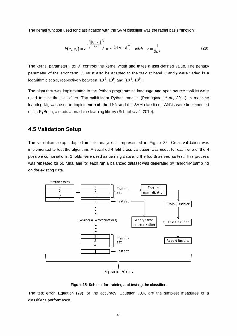
41
The kernel function used for classification with the SVM classifier was the radial basis function:
𝑘(𝒙𝑖 , 𝒙𝑗) = 𝑒−(
‖𝒙𝑖−𝒙𝑗‖2
2𝜎2 )
= 𝑒−(𝛾‖𝒙𝑖−𝒙𝑗‖2
) 𝑤𝑖𝑡ℎ 𝛾 =1
2𝜎2 (28)
The kernel parameter 𝛾 (or 𝜎) controls the kernel width and takes a user-defined value. The penalty
parameter of the error term, 𝐶, must also be adapted to the task at hand. 𝐶 and 𝛾 were varied in a
logarithmic scale, respectively between [10-2
, 108] and [10
-5, 10
3].
The algorithm was implemented in the Python programming language and open source toolkits were
used to test the classifiers. The scikit-learn Python module (Pedregosa et al., 2011), a machine
learning kit, was used to implement both the kNN and the SVM classifiers. ANNs were implemented
using PyBrain, a modular machine learning library (Schaul et al., 2010).
4.5 Validation Setup
The validation setup adopted in this analysis is represented in Figure 35. Cross-validation was
implemented to test the algorithm. A stratified 4-fold cross-validation was used: for each one of the 4
possible combinations, 3 folds were used as training data and the fourth served as test. This process
was repeated for 50 runs, and for each run a balanced dataset was generated by randomly sampling
on the existing data.
Figure 35: Scheme for training and testing the classifier.
The test error, Equation (29), or the accuracy, Equation (30), are the simplest measures of a
classifier’s performance.

42
𝑇𝑒𝑠𝑡 𝐸𝑟𝑟𝑜𝑟 = 𝑁𝑢𝑚𝑏𝑒𝑟 𝑜𝑓 𝑀𝑖𝑠𝑐𝑙𝑎𝑠𝑠𝑖𝑓𝑖𝑐𝑎𝑡𝑖𝑜𝑛𝑠
𝑁𝑢𝑚𝑏𝑒𝑟 𝑜𝑓 𝑇𝑒𝑠𝑡 𝑆𝑎𝑚𝑝𝑙𝑒𝑠 (29)
𝐴𝑐𝑐𝑢𝑟𝑎𝑐𝑦 = 𝑁𝑢𝑚𝑏𝑒𝑟 𝑜𝑓 𝐶𝑜𝑟𝑟𝑒𝑐𝑡 𝐶𝑙𝑎𝑠𝑠𝑖𝑓𝑖𝑐𝑎𝑡𝑖𝑜𝑛𝑠
𝑁𝑢𝑚𝑏𝑒𝑟 𝑜𝑓 𝑇𝑒𝑠𝑡 𝑆𝑎𝑚𝑝𝑙𝑒𝑠 (30)
To evaluate the classifier’s performance a couple of accuracy measures, besides the error rate, were
computed. Using the usual notation for true positives, true negatives, false positives and false
negatives (that is 𝑇𝑃, 𝑇𝑁, 𝐹𝑃 and 𝐹𝑁) we can define the precision (or positive predictive value) and
the recall (or sensitivity) as shown in equations (31) and (32). The F1 score also known as F-score or
F-measure is the harmonic mean of precision and sensitivity and can be obtained by equation (33).
𝑃𝑟𝑒𝑐𝑖𝑠𝑖𝑜𝑛 =𝑇𝑃
𝑇𝑃 + 𝐹𝑃 (31)
𝑅𝑒𝑐𝑎𝑙𝑙 =𝑇𝑃
𝑇𝑃 + 𝐹𝑁 (32)
𝐹1 =2𝑇𝑃
2𝑇𝑃 + 𝐹𝑃 + 𝐹𝑁 (33)

43
5. Experimental Setup and Results
5.1 Experimental Setup
The validation of the proposed methodology was performed on benchmark data and ECG acquisitions
performed in collaboration with Santa Marta Hospital, as described next.
5.1.1 BITalino Acquisitions
Acquisitions
ECG recordings were acquired with the BITalino at Santa Marta Hospital, in Lisbon, during the months
of June and July. Subjects were either inpatients or came to the hospital for diagnosis (stress test or
tilt table test) or rehabilitation purposes. All subjects gave written informed consent before the
acquisition (see Annex A). They were asked to hold one electrode in each hand, between thumb and
index finger. Simultaneous recordings were obtained with traditional 12-lead ECG and the BITalino
system to allow an accurate ECG interpretation. Since automatic rhythm classification was to be
performed, an attempt was made to acquire at least 60 seconds of data with the BITalino system. The
OpenSignals software, available at (Plux Wireless Biosignals, 2014) and allowing real time
visualization, was used to acquire the data.
During the acquisition process, it was clear that some rooms gave rise to a noisier ECG and the
BITalino system was far more affected by this noise than the standard 12-lead system. Another
difficulty encountered was the involuntary movement of some subjects, which resulted in ECGs with
artefacts. It was particularly difficult to acquire data when the subject suffered with tremors due to the
incapacity to keep the extremities still. Some subjects, although instructed otherwise, tended to hold
the electrodes too tight, which also resulted in muscular noise. The technicians operating the 12-lead
system complained about this situation since it also affected the standard ECG.
A total of 294 records were acquired, corresponding to 180 men with an age of approximately 46.78 ±
30.21 years and 114 women with an age of approximately 46.09 ± 30.65 years.
Annotations
Resorting to the standard 12-lead ECG, an experienced cardiologist interpreted the records in terms of
type of rhythm and other meaningful information. These annotations are presented in the Annex B
(Table 31). Naturally, the majority of the records had an underlying sinus rhythm. It was also common
to capture premature ventricular contractions and a few atrial premature beats were recorded. Both
these events can be recognized using lead I and thus are also visible in the BITalino ECG record. A
couple of sinus bradycardia and sinus tachycardia ECG segments were recorded. Unsurprisingly, the
more recurrent abnormal rhythm was the most common arrhythmia, atrial fibrillation. One can expect
to be able to recognize such arrhythmia simply with lead I. The same can be said about atrial flutter
although ECGs with this rhythm were much more rarely captured. Atrioventricular blocks and right or
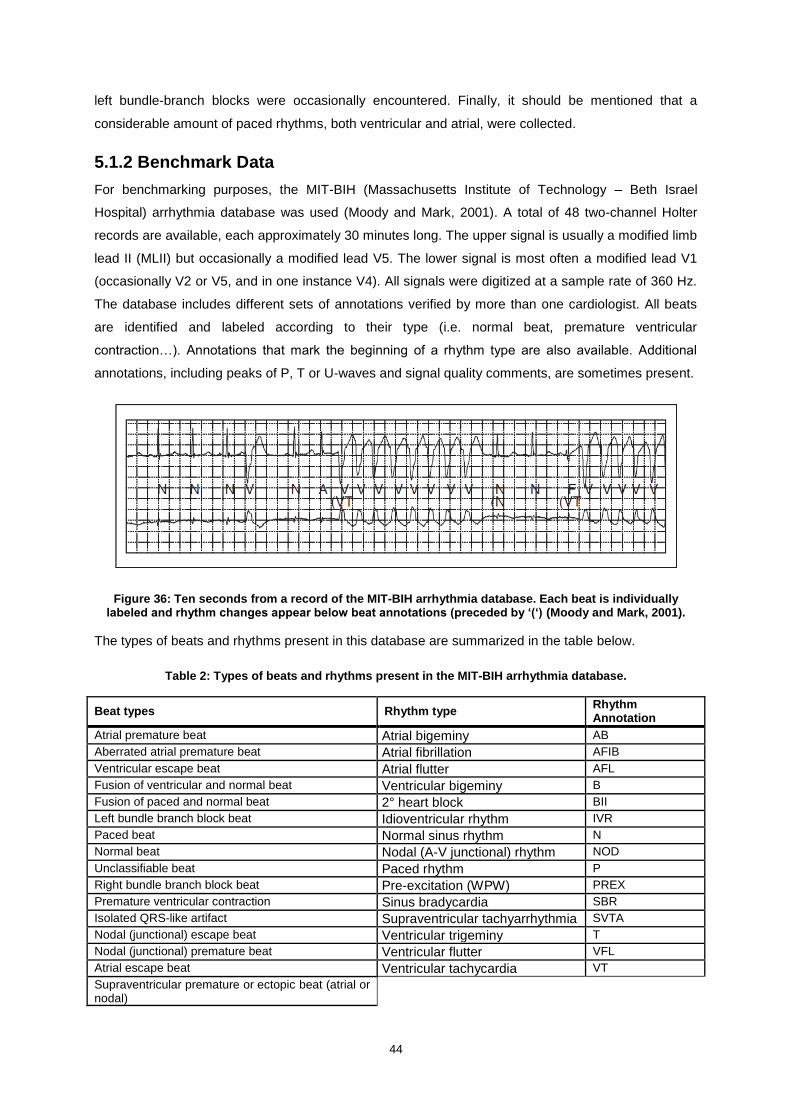
44
left bundle-branch blocks were occasionally encountered. Finally, it should be mentioned that a
considerable amount of paced rhythms, both ventricular and atrial, were collected.
5.1.2 Benchmark Data
For benchmarking purposes, the MIT-BIH (Massachusetts Institute of Technology – Beth Israel
Hospital) arrhythmia database was used (Moody and Mark, 2001). A total of 48 two-channel Holter
records are available, each approximately 30 minutes long. The upper signal is usually a modified limb
lead II (MLII) but occasionally a modified lead V5. The lower signal is most often a modified lead V1
(occasionally V2 or V5, and in one instance V4). All signals were digitized at a sample rate of 360 Hz.
The database includes different sets of annotations verified by more than one cardiologist. All beats
are identified and labeled according to their type (i.e. normal beat, premature ventricular
contraction…). Annotations that mark the beginning of a rhythm type are also available. Additional
annotations, including peaks of P, T or U-waves and signal quality comments, are sometimes present.
Figure 36: Ten seconds from a record of the MIT-BIH arrhythmia database. Each beat is individually labeled and rhythm changes appear below beat annotations (preceded by ‘(‘) (Moody and Mark, 2001).
The types of beats and rhythms present in this database are summarized in the table below.
Table 2: Types of beats and rhythms present in the MIT-BIH arrhythmia database.
Beat types Rhythm type Rhythm Annotation
Atrial premature beat Atrial bigeminy AB
Aberrated atrial premature beat Atrial fibrillation AFIB
Ventricular escape beat Atrial flutter AFL
Fusion of ventricular and normal beat Ventricular bigeminy B
Fusion of paced and normal beat 2° heart block BII
Left bundle branch block beat Idioventricular rhythm IVR
Paced beat Normal sinus rhythm N
Normal beat Nodal (A-V junctional) rhythm NOD
Unclassifiable beat Paced rhythm P
Right bundle branch block beat Pre-excitation (WPW) PREX
Premature ventricular contraction Sinus bradycardia SBR
Isolated QRS-like artifact Supraventricular tachyarrhythmia SVTA
Nodal (junctional) escape beat Ventricular trigeminy T
Nodal (junctional) premature beat Ventricular flutter VFL
Atrial escape beat Ventricular tachycardia VT
Supraventricular premature or ectopic beat (atrial or nodal)

45
For this analysis only MLII records were used (records number 102 and 104 were therefore excluded).
5.2 Results R Peak Detection
In order to evaluate the performance of the algorithm used for R-peak detection, the MIT-BIH
arrhythmia database was used, taking advantage of the beat annotations present.
The Waveform Database (WFDB) Software Package, available in (Moody, 2014), was used for
validation. For each ECG record, R peaks were detected and an annotation file containing their
positions was generated. These positions were then compared to the reference annotations from the
database. Standard comparison options were used: the comparison started 5 minutes after the
beginning of the record and the match window, maximum absolute difference in annotation times
allowable for matching annotations, was set to 0.15 second.
The results obtained, in terms of sensitivity and positive predictive value, are illustrated in Figure 37 for
different threshold coefficients TH (see equation 24). As stated in section 4.1.3, larger TH values lead
to a higher number of correct detections whereas smaller values are characterized by a small rate of
false detections. A performance curve as a function of this threshold was therefore constructed.
Figure 37: Sensitivity-positive predictive value curve for different threshold (TH) values.
A threshold coefficient of 0.25, corresponding to sensitivity and positive predictive values of 99.59 and
99.69%, respectively, was used for the remaining tests.
In order to understand which types of rhythms were more prone to detection errors, the following
experiment was implemented. Records were first split according to their rhythm so that rhythm type
did not vary within the segment (although beat types did vary). Then, for each segment, peaks were
detected. Using again a match window of 0.15 second, annotations were compared to the reference
annotations. Sensitivity and positive predictive values obtained for each rhythm type are summarized
in Table 3.

46
Table 3: Sensitivity and positive predictive value of R peak detection according to the type of rhythm.
Rhythm type Sensitivity (%) Positive Predictive Value (%)
Atrial bigeminy 100 100
Atrial fibrillation 99.02 99.71
Atrial flutter 98.50 99.42
Ventricular bigeminy 99.61 99.85
2° heart block 100 100
Idioventricular rhythm 100 100
Normal sinus rhythm 99.57 99.71
Nodal (A-V junctional) rhythm 100 100
Paced rhythm 99.82 99.87
Pre-excitation (WPW) 100 100
Sinus bradycardia 100 99.55
Supraventricular tachyarrhythmia 100 100
Ventricular trigeminy 99.04 99.70
Ventricular flutter 96.25 98.47
Total 99.50 99.71
Analyzing the table above it seems that detection rates vary among rhythm type. The smallest values
of sensitivity and positive predictive values were obtained for ventricular tachycardia. Trigeminy and
bigeminy, which are characterized by an alternation of normal and ventricular beats, also present
lower sensitivity values. Finally, the sensitivity for segments of atrial flutter and atrial fibrillation is also
below average.
Additional information, concerning the amount of correct and missed detections per beat type, was
gathered and is presented in Table 4. It should also be mentioned that a total of 632 false positives
were obtained.
Table 4: Results of the R peak detection algorithm per beat type.
Beat type Correct
detections Missed
detections Error rate (%)
Atrial premature beat 2540 1 0.04
Aberrated atrial premature beat 100 50 33.33
Ventricular escape beat 106 0 0
Fusion of ventricular and normal beat 798 5 0.62
Fusion of paced and normal beat 259 1 0.38
Left bundle branch block beat 8055 20 0.25
Paced beat 3619 1 0.03
Normal beat 74178 136 0.18
Unclassifiable beat 7 8 53.33
Right bundle branch block beat 7259 0 0
Premature ventricular contraction 6914 210 2.95
Isolated QRS-like artifact 41 91 68.94
Nodal (junctional) escape beat 229 0 0
Nodal (junctional) premature beat 83 0 0
Supraventricular premature or ectopic beat (atrial or nodal) 2 0 0
Atrial escape beat 16 0 0
Total 104206 523 0.50

47
Interesting conclusions can be draw from the information shown above. It is clear that some beat
types are much more easily detected than others. Whilst the error rate is below 1% for the majority of
beats, there are some noteworthy exceptions. The detection of premature ventricular contractions has
an error rate close to 3%, which explains the results obtained previously for ventricular tachycardia,
bigeminy and trigeminy. The worst results correspond however to aberrated atrial premature beats
and unclassifiable beats, with error rates of, respectively, 33.33 and 53.33%. Referring to Figure 38
and Figure 39 it is understandable why such high error rates were obtained. Concerning false positive
errors, two examples are shown in Figure 40. In the first case, where the R peak is inverted, the
algorithm detected a P wave. In the second, premature ventricular contractions occurred, and the
algorithm considered a T wave as an R peak. Other situations where false positive occurred consisted
of records with artefacts.
Figure 38: Example of two aberrated atrial premature beats (a) that were not detected by the segmentation algorithm.
Figure 39: Example of one unclassifiable beat (Q) that was not detected by the segmentation algorithm.

48
Figure 40: Example of two false positive errors. In the left, where R peaks are inverted, a P wave is detected. In the right, where PVCs occur, a T wave is detected.
5.3 Rhythm Classification on Benchmark Database
5.3.1 Database Assembly
The same database used to validate the R peak detection algorithm was used in this analysis. In order
to perform rhythm classification, each record was split into multiple segments according to rhythm
annotations. Additional cuts were made in a non-overlapping manner to obtain segments of predefined
length. The total number of segments obtained for each type of rhythm and segment length is
presented in Table 5. For the features based on the location of the R peaks, the position annotations
present on the database were used. This assures that the performance of the algorithm is not affected
by possible mistakes on the detection of the peaks.
Table 5: Number of segments per rhythm type for different segment’s lengths.
Rhythm type 10 s
segments 30 s
segments 60 s
segments
AB 7 2 1
AFIB 752 226 98
AFL 60 14 6
B 144 31 7
BII 68 21 9
IVR 12 3 1
N 6046 1920 911
NOD 7 0 0
P 316 99 45
PREX 36 6 1
SBR 180 60 30
SVTA 12 1 0
T 72 12 3
VFL 12 3 1
VT 8 2 0
Total 7732 2400 1113

49
5.3.2 Normal Sinus Rhythm vs. Atrial Fibrillation
The first set of experiments focused on the distinction of normal sinus rhythm and the most common
arrhythmia, atrial fibrillation (AF). The three feature sets described in the previous chapter were
considered, first individually and then in combination. The parameters of the classifiers were varied in
order to find the most suitable values for each case. Segments with a length of 60 seconds were used.
As shown in Table 5, 98 atrial fibrillation segments and 911 normal sinus rhythm segments are
available. Thus, for each run, 98 segments of each class are selected and the validation process is
carried out.
Time parameters (feature set C)
A first attempt was made to distinguish between normal sinus rhythm and AF ECG segments relying
only on heart rate related features (feature set C). As stated in section 4.4, the classifiers’ parameters
were varied to find the most suitable values. For the SVM, the penalty parameter of the error term, 𝐶,
and the kernel parameter, 𝛾, were varied in a logarithmic scale, respectively between [10-2
, 108] and
[10-5
, 103]. For the kNN, the number of neighbors considered for classification, 𝑘, was varied between
1 and 15. Regarding the ANN, the number of hidden neurons was varied, in this case, between 3 and
12. The classifiers’ parameters that led to the best performance are summarized in Table 6. For the
ANN the best result corresponded to standardized features with 10 neurons in the hidden layer. For
the kNN classifier, the best performance was achieved when features were standardized and three
neighbors were considered. Figure 41 and Figure 42 show, respectively, the variation of test error with
the number of hidden neurons (for the ANN), and the number of neighbors (for the kNN). Concerning
the SVM classifier, values of 1 and 10 respectively for the penalty, 𝐶, and kernel, 𝛾, parameters led to
a more successful classification. Figure 43 shows the heat map of the accuracy of the SVM classifier
for different values of the penalty and kernel parameters.
Figure 41: Mean and standard deviation of the test error as a function of the number of neurons in the hidden layer for the two normalization schemes, for feature set C.

50
Figure 42: Mean and standard deviation of the test error as a function of the number of neighbors used for classification for the two normalization schemes, for feature set C.
Figure 43: Heat map showing the accuracy of the SVM classifier for multiple values of C and gamma, for feature set C.
We can see that, for the ANN, standardizing features resulted better than scaling them. In terms of
hidden neurons, the range 6 to 10 offered very similar results, with a poorer performance when
selecting fewer or more neurons. For the kNN classifier, the two types of normalization schemes
offered similar results. The test error was smaller when using three neighbors than a single one and
then increased when more neighbors were considered. Regarding the SVM, the majority of 𝐶 and 𝛾
combinations resulted in accuracy above 85%. The exception was for small values of 𝐶 and large
values of 𝛾, which achieved far worse accuracies.

51
Table 6: Best classifiers’ parameters for each classification task.
Feature set Classifier Normalization Parameters
A
ANN Scaling 55 Hidden Neurons
kNN Standardization 𝑘 = 1
SVM Standardization 𝐶 = 103 ; 𝛾 = 10−2
B
ANN
Standardization
15 Hidden Neurons
kNN 𝑘 = 1
SVM 𝐶 = 102 ; 𝛾 = 1
C
ANN
Standardization
10 Hidden Neurons
kNN 𝑘 = 3
SVM 𝐶 =1 ; 𝛾 = 10
A + C
ANN Scaling 35 Hidden Neurons
kNN Scaling 𝑘 = 1
SVM Standardization 𝐶 = 108 ; 𝛾 = 10−2
B + C
ANN
Standardization
14 Hidden Neurons
kNN 𝑘 = 1
SVM 𝐶 = 10 ; 𝛾 = 1
The results obtained for the three classifiers are summarized in Table 7, showing mean values and
standard deviations computed over 50 runs (see section 4.5). Highlighted in bold are the highest
values of precision, recall and F-score for each class, and the minimum test error achieved.
Table 7: Results obtained with feature set C.
Classifier Rhythm Precision (%) Recall (%) F-score (%) Test error (%)
ANN Normal 98.66 ± 1.00 90.31 ± 1.86 94.21 ± 1.22
5.49 ± 1.15 Atrial Fibrillation 91.27 ± 1.62 98.72 ± 0.98 94.78 ± 1.08
kNN Normal 97.93 ± 1.34 91.4 ± 2.61 94.44 ± 1.77
5.31 ± 1.65 Atrial Fibrillation 92.19 ± 2.22 97.98 ± 1.34 94.90 ± 1.55
SVM Normal 96.79 ± 1.41 94.23 ± 2.20 95.39 ± 1.55
4.53 ± 1.50 Atrial Fibrillation 94.56 ± 2.01 96.71 ± 1.50 95.53 ± 1.47
Overall, the SVM classifier was the one that performed better, achieving a test error of 4.53 ± 1.50%.
ANN and kNN classifiers have a similar performance in terms of test error. For the ANN it is interesting
to note that precision and recall values, respectively for normal and AF rhythms, are considerably high
(approximately 99%).
The experimental results based on spectral features are presented next.
Average PSD Values (feature set A)
Feature set A, containing the 42 values obtained by averaging the PSD of the wavelet decomposition,
was considered first. Figure 44, Figure 45 and Figure 46 illustrate the tests performed to assess the
most suitable classifiers’ parameters. The best results, presented in Table 8, were obtained with the
parameters specified in Table 6. It should be mentioned that in this case, due to the large number of
features, the number of hidden neurons was varied between 10 and 70, in steps of 5.

52
Figure 44: Mean and standard deviation of the test error as a function of the number of neurons in the hidden layer for the two normalization schemes, for feature set A.
Figure 45: Mean and standard deviation of the test error as a function of the number of neighbors used for classification for the two normalization schemes, for feature set A.
Figure 46: Heat map showing the accuracy of the SVM classifier for multiple values of C and gamma, for feature set A.

53
Analyzing Figure 44 it is clear that scaling the features results better than standardizing them when
using a larger number of neurons in the hidden layer. It is also noteworthy that, in comparison with the
previous feature set, a much larger number of neurons are needed to achieve the best performance.
Obviously, this largely influences the time needed for training the network. Regarding the kNN, the two
normalization schemes offer again similar results. In this case, the error rate increased when
considering more neighbors for classification. For the SVM classifier, the higher accuracies
corresponded to values of 𝐶 and 𝛾 respectively between [102, 10
8] and [10
-2, 10
-1].
Table 8: Results obtained with feature set A.
Classifier Rhythm Precision (%) Recall (%) F-score (%) Test error (%)
ANN Normal 96.90 ± 1.83 86.36 ± 3.08 91.06 ± 1.83
8.29 ± 1.57 Atrial Fibrillation 88.18 ± 2.28 97.07 ± 1.84 92.24 ± 1.41
kNN Normal 96.92 ± 1.11 91.27 ± 3.08 93.87 ± 1.88
5.87 ± 1.72 Atrial Fibrillation 92.04 ± 2.62 96.99 ± 1.15 94.35 ± 1.60
SVM Normal 95.56 ± 1.62 93.77 ± 2.00 94.54 ± 1.46
5.39 ± 1.44 Atrial Fibrillation 94.10 ± 1.85 95.45 ± 1.70 94.66 ± 1.44
The smallest test error was obtained with the SVM classifier: 5.39 ± 1.44%. For the kNN, a test error
below 6% was also achieved. The ANN proved to be the less capable classifier for distinguishing
between the two rhythms. Additionally, it should be mentioned that the training process associated
with this classifier was lengthier, due, in part, to the high number of hidden neurons required.
Interestingly, precision and recall values, respectively for normal and AF, are very similar for kNN and
ANN. However, the latter presents considerably smaller values of recall, for normal rhythm, and
precision, for AF.
Large Range Power Features (feature set B)
The 7 large range power features (feature set B) were then tested in this binary classification problem.
Table 6 indicates the best classifiers’ parameters. Figure 47, Figure 48, and Figure 49 illustrate the
multiple tests performed to obtain these values.
Figure 47: Mean and standard deviation of the test error as a function of the number of neurons in the hidden layer for the two normalization schemes, for feature set B.
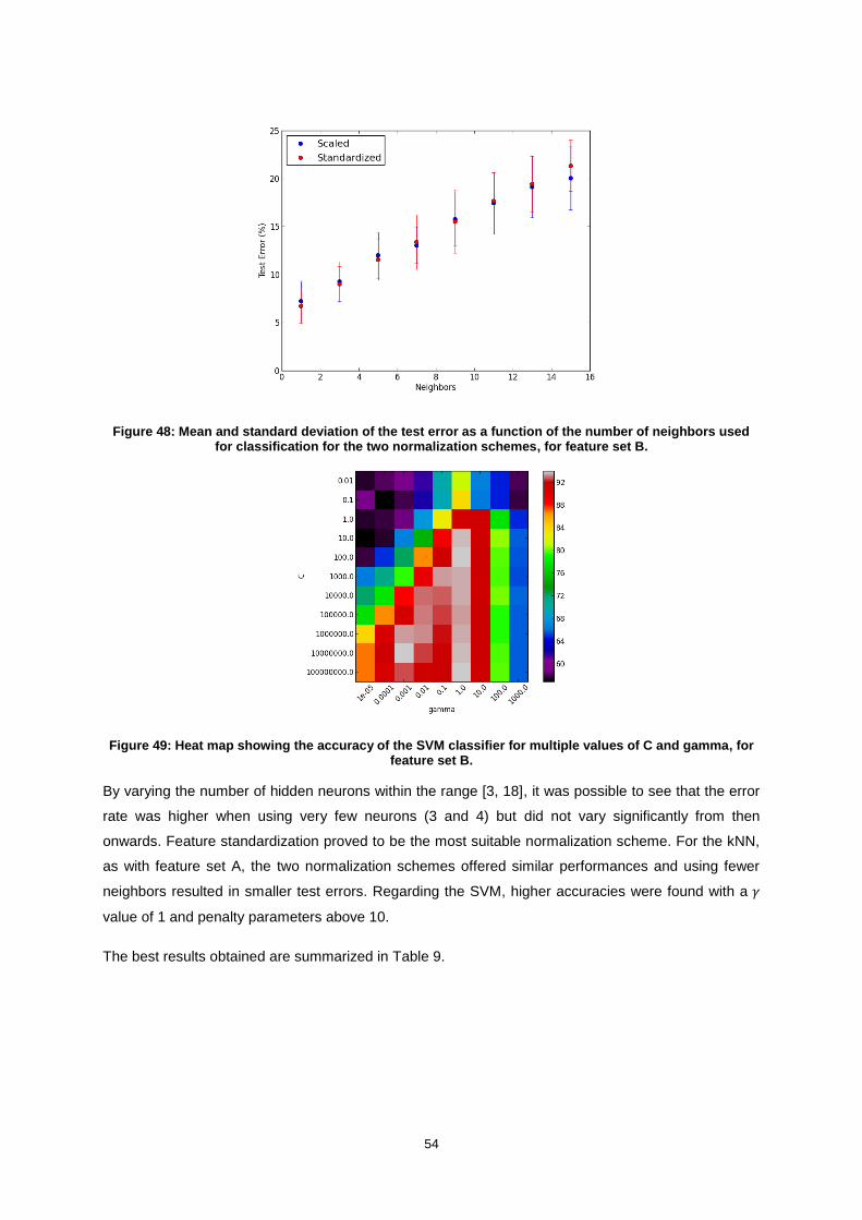
54
Figure 48: Mean and standard deviation of the test error as a function of the number of neighbors used for classification for the two normalization schemes, for feature set B.
Figure 49: Heat map showing the accuracy of the SVM classifier for multiple values of C and gamma, for feature set B.
By varying the number of hidden neurons within the range [3, 18], it was possible to see that the error
rate was higher when using very few neurons (3 and 4) but did not vary significantly from then
onwards. Feature standardization proved to be the most suitable normalization scheme. For the kNN,
as with feature set A, the two normalization schemes offered similar performances and using fewer
neighbors resulted in smaller test errors. Regarding the SVM, higher accuracies were found with a 𝛾
value of 1 and penalty parameters above 10.
The best results obtained are summarized in Table 9.

55
Table 9: Results obtained with feature set B.
Classifier Rhythm Precision (%) Recall (%) F-score (%) Test error (%)
ANN Normal 95.24 ± 2.30 86.16 ± 3.60 90.18 ± 2.49
9.21 ± 2.23 Atrial Fibrillation 87.83 ± 2.84 95.41 ± 2.33 91.26 ± 2.06
kNN Normal 96.73 ± 1.31 89.70 ± 3.38 92.91 ± 2.01
6.73 ± 1.80 Atrial Fibrillation 90.75 ± 2.80 96.84 ± 1.31 93.56 ± 1.63
SVM Normal 96.74 ± 1.46 91.13 ± 2.67 93.70 ± 1.76
6.04 ± 1.64 Atrial Fibrillation 91.93 ± 2.31 96.78 ± 1.49 94.17 ± 1.55
Once again, the best results, in terms of test error, were obtained with the SVM classifier. The ANN
classifier offered the worst performance. For all classifiers, recall values were considerably higher, and
not very different, for AF segments. The differences in test error are therefore due to the values of
recall obtained for normal segments (or, equivalently, to the values of precision for AF segments).
Figure 50 shows the performance, in terms of test error, of the three classifiers, for the three feature
sets used. It is clear that time domain features performed better than spectral features. Feature set A,
containing average values over sub-bands, achieved better results than feature set B, containing the
large range power features. In terms of classifiers, SVM proved to be the most promising choice whilst
ANN achieved the worst results for all sets of features.
Figure 50: Means and standard deviations of test errors for feature sets C (time parameters), A (average PSD values) and B (large range power values).
The next step was to assess whether combining spectral and time domain features could improve the
classifiers’ performance.
Average PSD Values + Time Parameters (feature sets A + C)
The results obtained when combining feature sets A and C are presented in Table 10. Figure 51,
Figure 52 and Figure 53 illustrate the tests performed to determine the best classifiers’ parameters
(summarized in Table 6).
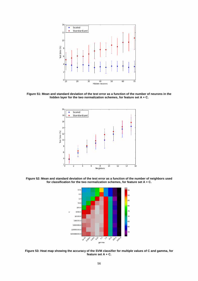
56
Figure 51: Mean and standard deviation of the test error as a function of the number of neurons in the hidden layer for the two normalization schemes, for feature set A + C.
Figure 52: Mean and standard deviation of the test error as a function of the number of neighbors used for classification for the two normalization schemes, for feature set A + C.
Figure 53: Heat map showing the accuracy of the SVM classifier for multiple values of C and gamma, for feature set A + C.

57
Regarding the ANN, scaling the features was the most suitable approach. Interestingly, the results
obtained when standardizing the features seem to show that this normalization scheme works worst
for a larger number of hidden neurons. Scaling the features also resulted in a smaller test error for the
kNN classifier. Regarding the SVM, very high values of 𝛾 and small values of 𝐶 achieved the smallest
accuracies. A large number of combinations offered accuracy values above 95%.
Table 10: Results obtained with feature set A + C.
Classifier Rhythm Precision (%) Recall (%) F-score (%) Test error (%)
ANN Normal 99.17 ± 0.95 94.55 ± 2.57 96.73 ± 1.58
3.13 ± 1.46 Atrial Fibrillation 94.98 ± 2.22 99.19 ± 0.93 96.98 ± 1.37
kNN Normal 98.29 ± 0.72 94.35 ± 2.48 96.19 ± 1.38
3.67 ± 1.27 Atrial Fibrillation 94.77 ± 2.17 98.31 ± 0.72 96.44 ± 1.19
SVM Normal 98.23 ± 1.23 96.69 ± 2.05 97.39 ± 1.40
2.55 ± 1.33 Atrial Fibrillation 96.89 ± 1.80 98.20 ± 1.25 97.49 ± 1.28
This combination of spectral and time domain features achieved, for all classifiers, accuracies above
94%. The SVM classifier stood out, with a mean test error of 2.55%. Very high values of precision and
recall, respectively for normal sinus rhythm and AF, were obtained with the ANN (above 99%). It
should be mentioned that the mean training error obtained with this classifier was 0.97 ± 0.59%.
Therefore it may be the case that the network has specialized its behavior for the training patterns,
losing some of its generalization ability.
Large Range Power Features + Time Parameters (feature sets B + C)
The tests performed to select the best classifiers’ parameters when using feature sets B and C are
illustrated in Figure 54, Figure 55, and Figure 56, respectively for ANN, kNN and SVM. Again, the
most suitable parameters are summarized in Table 6.
Figure 54: Mean and standard deviation of the test error as a function of the number of neurons in the hidden layer for the two normalization schemes, for feature set B + C.

58
Figure 55: Mean and standard deviation of the test error as a function of the number of neighbors used for classification for the two normalization schemes, for feature set B + C.
Figure 56: Heat map showing the accuracy of the SVM classifier for multiple values of C and gamma, for feature set B + C.
Regarding the ANN, standardizing the features offered better results when compared to scaling them.
The test error oscillated with the number of hidden neurons and the smaller value was obtained with
14 neurons. For the kNN, similar results were obtained for the two normalization schemes and using a
single neighbor was the most suitable choice. Referring to Figure 56 it is clear that the SVM classifier
achieved the best performance when 𝛾 was set to 1 and 𝐶 was above this value.
The results obtained are presented in Table 11.
Table 11: Results obtained with feature set B + C.
Classifier Rhythm Precision (%) Recall (%) F-score (%) Test error (%)
ANN Normal 99.36 ± 0.58 94.67 ± 2.30 96.89 ± 1.26
2.98 ± 1.16 Atrial Fibrillation 95.11 ± 1.98 99.37± 0.57 97.14 ± 1.08
kNN Normal 99.06 ± 0.60 95.75 ± 2.10 97.31 ± 1.17
2.60 ± 1.10 Atrial Fibrillation 96.07 ± 1.85 99.04 ± 0.67 97.48 ± 1.04
SVM Normal 98.64 ± 0.83 99.59 ± 0.64 99.10 ± 0.64
0.92 ± 0.66 Atrial Fibrillation 99.61 ± 0.62 98.57 ± 0.92 99.06 ± 0.68

59
With this feature set, all three classifiers achieved test errors below 3%. The best results were
obtained with the SVM with an accuracy of 99.08% and F-scores above 99% for both classes.
Although the worst results, in terms of test error, were obtained with the ANN, a very high recall rate
was achieved for AF: 99.37%. This can be a valuable characteristic since it may be important to detect
all AF events, even if this encompasses a larger number of false positive errors. It should again be
mentioned that the training error for the ANN was considerably smaller than the test error: 0.91 ±
0.47%.
From the results presented above it became clear that combining time domain and spectral features
considerably improves the classifiers’ performance. This was true for the two combinations and for all
three classifiers. The best results were obtained when combining feature sets B and C and using the
SVM classifier, as shown in Figure 57.
Figure 57: Means and standard deviations of test errors for feature sets A + C and B + C.
Influence of segments’ length
The study of features presented above was carried out with ECG segments of 60 seconds. The
influence of the segments’ length on the performance of the classifiers is explored here. Features
used for classification were the ones that held better results: large range power features in
combination with time parameters (feature sets B + C). The classifiers’ parameters were set to the
values obtained previously with this set of features (see Table 6).
As shown in Table 5 the number of segments of different lengths varies greatly. This fact must be
taken into account when performing this analysis; therefore the two following experiments were
considered. First, for each classifier, segments’ length of 60, 30 and 10 seconds were used while
using as many samples per rhythm as available (i.e. 98, 226 and 752 respectively for 60, 30 and 10
seconds). Secondly, the number of samples was kept unchanged, 98, varying only the segments’

60
length. The results obtained are presented in Table 12, Table 13 and Table 14, respectively for ANN,
kNN and SVM classifiers. A graphical representation of the test error for both experiments and all
classifiers is shown in Figure 58.
Table 12: Results obtained when varying the segments’ length for the ANN classifier.
Length (s)
Samples per rhythm
Rhythm Precision (%)
Recall (%)
F-score (%)
Test error (%)
60 98 Normal 99.36 ± 0.58 94.67 ± 2.30 96.89 ± 1.26
2.98 ± 1.16 Atrial Fibrillation 95.11 ± 1.98 99.37± 0.57 97.14 ± 1.08
30
98 Normal 97.84 ± 1.48 92.65 ± 2.18 95.06 ± 1.49
4.76 ± 1.42 Atrial Fibrillation 93.24 ± 1.92 97.86 ± 1.49 95.40 ± 1.36
226 Normal 98.36 ± 0.76 96.28 ± 1.36 97.27 ± 0.79
2.68 ± 0.76 Atrial Fibrillation 96.43 ± 1.26 98.36 ± 0.77 97.36 ± 0.74
10
98 Normal 94.94 ± 2.27 89.75 ± 2.21 92.09 ± 1.75
7.64 ± 1.70 Atrial Fibrillation 90.58 ± 1.94 94.97 ± 2.31 92.58 ± 1.67
752 Normal 98.54 ± 0.41 96.19 ± 0.56 97.34 ± 0.34
2.62 ± 0.34 Atrial Fibrillation 96.30 ± 0.52 98.56 ± 0.41 97.41 ± 0.33
Table 13: Results obtained when varying the segments’ length for the kNN classifier.
Length (s)
Samples per rhythm
Rhythm Precision (%)
Recall (%)
F-score (%)
Test error (%)
60 98 Normal 99.06 ± 0.60 95.75 ± 2.10 97.31 ± 1.17
2.60 ± 1.10 Atrial Fibrillation 96.07 ± 1.85 99.04 ± 0.67 97.48 ± 1.04
30
98 Normal 98.51 ± 1.37 94.15 ± 2.10 96.21 ± 1.45
3.67 ± 1.41 Atrial Fibrillation 94.56 ± 1.89 98.51 ± 1.42 96.43 ± 1.38
226 Normal 98.99 ± 0.57 96.68 ± 1.10 97.80 ± 0.71
2.16 ± 0.69 Atrial Fibrillation 96.81 ± 1.04 99.00 ± 0.56 97.87 ± 0.68
10
98 Normal 96.23 ± 1.97 91.05 ± 2.52 93.42 ± 1.79
6.36 ± 1.73 Atrial Fibrillation 91.75 ± 2.24 96.24 ± 2.04 93.82 ± 1.69
752 Normal 98.53 ± 0.30 96.13 ± 0.55 97.31 ± 0.36
2.65 ± 0.35 Atrial Fibrillation 96.24 ± 0.52 98.56 ± 0.30 97.38 ± 0.34
Table 14: Results obtained when varying the segments’ length for the SVM classifier.
Length (s)
Samples per rhythm
Rhythm Precision (%)
Recall (%)
F-score (%)
Test error (%)
60 98 Normal 98.64 ± 0.83 99.59 ± 0.64 99.10 ± 0.64
0.92 ± 0.66 Atrial Fibrillation 99.61 ± 0.62 98.57 ± 0.92 99.06 ± 0.68
30
98 Normal 96.56 ± 1.46 98.18 ± 1.26 97.30 ± 1.02
2.73 ± 1.04 Atrial Fibrillation 98.23 ± 1.21 96.35 ± 1.62 97.22 ± 1.07
226 Normal 97.93 ± 0.74 98.91 ± 0.57 98.41 ± 0.46
1.61 ± 0.47 Atrial Fibrillation 98.92 ± 0.57 97.88 ± 0.77 98.38 ± 0.48
10
98 Normal 91.65 ± 2.31 95.43 ± 2.34 93.35 ± 2.07
6.83 ± 2.11 Atrial Fibrillation 95.41 ± 2.24 90.92 ± 2.59 92.95 ± 2.19
752 Normal 97.51 ± 0.42 97.72 ± 0.48 97.61 ± 0.34
2.40 ± 0.34 Atrial Fibrillation 97.73 ± 0.47 97.49 ± 0.43 97.60 ± 0.34

61
Figure 58: Mean and standard deviation of the test error as a function of the segments’ length.
A few observations can be made from the results presented above. First, the results obtained for
segments of 30 and 10 seconds are better when using all samples available as opposed to using only
98 samples. This is not surprising: for a fixed segment length, the performance of the classifiers is
improved when more samples are provided for training.
For 10 seconds segments, when using all samples, the performance of the three classifiers is very
similar. Mean test errors below 2.65% with small standard deviations are obtained in this case.
Analyzing each classifier individually, interesting differences can be noted. Regarding the SVM
classifier, its performance worsens by reducing the segments’ length. This is true when using always
the same amount of samples, but also, to a lesser extent, when using all available samples. For the
kNN classifier, when using all samples, the test error decreases for segments of 30 seconds but
increases again when 10 seconds segments are used. The ANN classifier registers slight
improvements for segments of 30 and 10 seconds if more samples are used for train and test.
From these observations it is clear that reducing the segments’ length results in a loss of information,
which affects the classifiers’ performance. Depending on the classifier and the length of the segments,
this loss of information is, in part, compensated by a larger number of samples available for training. It
therefore seems as if there may be an ‘ideal’ segment length which will represent a compromise
between the information that can be extracted and the total number of segments available. This ‘ideal’
length will be different for each classifier.
Influence of R peak detection
All the experiments carried out until this point used reference R peak annotations, included in the
database. This allowed us to evaluate the performances of the classification algorithm in such a way
that it was not affected by segmentation errors. It is now important to check the real influence of these
R peak detection errors. In order to do so, the classification algorithm was reapplied, using this time R

62
peak annotations given by the segmentation algorithm described in the methodology section. The
results obtained are summarized in Table 15 and the difference between these results and the ones
obtained previously are illustrated in Figure 59.
Table 15: Results obtained with feature set B + C using non-reference R peak annotations.
Classifier Rhythm Precision (%) Recall (%) F-score (%) Test error (%)
ANN Normal 99.01 ± 0.76 93.67 ± 2.44 96.18 ± 1.34
3.65 ± 1.23 Atrial Fibrillation 94.22 ± 2.10 99.02 ± 0.76 96.49 ± 1.14
kNN Normal 98.91 ± 0.68 95.32 ± 2.05 97.03 ± 1.16
2.88 ± 1.08 Atrial Fibrillation 95.64 ± 1.81 98.93 ± 0.69 97.21 ± 1.02
SVM Normal 98.65 ± 0.72 98.98 ± 0.89 98.79 ± 0.61
1.22 ± 0.61 Atrial Fibrillation 99.02 ± 0.85 98.57 ± 0.81 98.76 ± 0.62
Figure 59: Comparison of rhythm classification error rate when using reference annotations and the segmentation algorithm.
Analyzing the figure above, it is clear that the results of the segmentation algorithm influence the
performance of the classification. For all classifiers, the test error increased when including the R peak
detection algorithm in the analysis. However, the results are still considerably good and the difference
is not large. We can conclude that, although improvements can be achieved, the segmentation
algorithm is reliable enough. It should nonetheless be expected that, with noisier data (e.g.
acquisitions with the BITalino at the fingers), the segmentation will affect the results in a larger extent.
5.3.3 Multiple Rhythms
The first set of tests focused only on distinguishing normal sinus rhythm from the most common
arrhythmia, atrial fibrillation. To test the performance of the algorithm in a more realistic situation, it is
necessary to include other types of rhythms in the classification task. The results obtained with
multiple rhythms are presented in this section. A few tests were performed maintaining a length of 60
seconds but, in order to have enough samples to include more rhythms, the segments’ length was
then shortened. The results presented here were obtained using the features that held best results:

63
large range power features in combination with time parameters (feature sets B and C). The
classifiers’ parameters were set to the corresponding values.
60 seconds segments
For segments of 60 seconds, and referring to Table 5, it is clear that there are not many samples of
different rhythms. However, by including paced rhythms, besides normal and AF segments, 45
samples per rhythm can still be used. The results obtained for this ternary classification problem are
presented in Table 16.
Table 16: Results obtained with feature sets B + C in the distinction of three rhythms.
Classifier Rhythm Precision (%) Recall (%) F-score (%) Test error (%)
ANN
Normal 98.57 ± 1.44 88.70 ± 4.82 93.05 ± 2.89
4.25 ± 1.65 Atrial Fibrillation 91.45 ± 3.46 98.54 ± 1.49 94.67 ± 2.02
Paced 98.76 ± 1.52 100.0 ± 0.0 99.35 ± 0.81
kNN
Normal 98.98 ± 1.35 91.74 ± 4.10 95.00 ± 2.64
3.10 ± 1.60 Atrial Fibrillation 93.87 ± 2.84 98.97 ± 1.36 96.22 ± 1.93
Paced 98.77 ± 1.48 100.0 ± 0.0 99.35 ± 0.78
SVM
Normal 97.99 ± 1.88 97.78 ± 1.90 97.79 ± 1.59
1.46 ± 1.05 Atrial Fibrillation 97.98 ± 1.68 98.5 ± 1.51 98.16 ± 1.36
Paced 100.0 ± 0.0 99.34 ± 1.19 99.65 ± 0.62
The number of samples used for training and testing the classifier was significantly reduced by
including paced rhythms (98 samples per rhythm for sinus rhythm versus atrial fibrillation, 45 samples
when the three rhythms are considered). The performance of the classifiers declined when compared
to the binary classification problem, but the results are still interesting. Again, SVM achieved the best
performance, followed by kNN, whilst the results for the ANN were worse. It is interesting to note that
very high rates of recognition of paced rhythm were obtained. For all three classifiers precision and
recall values were above 98.7%, including a recall of 100% for kNN and ANN, and a precision of
100% for the SVM. The main difference between SVM and the two other classifiers was that the first
managed to achieve high values of precision and recall respectively for atrial fibrillation and normal
sinus rhythm.
An additional classification problem was addressed considering the following four rhythms: normal
sinus rhythm, AF, paced rhythm and sinus bradycardia. A total of 30 samples per rhythm was selected
in each run. The results obtained are presented in Table 17.

64
Table 17: Results obtained with feature sets B + C in the distinction of four rhythms.
Classifier Rhythm Precision (%) Recall (%) F-score (%) Test error (%)
ANN
Normal 97.16 ± 3.46 82.54 ± 7.65 88.32 ± 5.54
5.71 ± 2.23 Atrial Fibrillation 86.64 ± 4.95 96.99 ± 3.30 91.09 ± 3.45
Paced 98.44 ± 2.10 99.86 ± 1.0 99.08 ± 1.33
Sinus bradycardia 98.66 ± 2.07 97.79 ± 1.59 98.09 ± 1.51
kNN
Normal 97.91 ± 2.83 82.72 ± 7.28 88.77 ± 5.14
5.18 ± 2.23 Atrial Fibrillation 87.32 ± 4.92 98.14 ± 2.92 91.98 ± 3.48
Paced 98.14 ± 2.15 100.0 ± 0.0 99.00 ± 1.15
Sinus bradycardia 99.48 ± 1.24 98.46 ± 1.67 98.90 ± 1.21
SVM
Normal 95.05 ± 2.92 94.41 ± 3.33 94.39 ± 2.50
3.24 ± 1.25 Atrial Fibrillation 94.39 ± 3.37 97.47 ± 2.62 95.64 ± 2.56
Paced 99.58 ± 1.05 98.52 ± 2.15 98.97 ± 1.29
Sinus bradycardia 99.63 ± 1.00 96.65 ± 0.22 98.02 ± 0.51
By including a fourth rhythm, and consequently decreasing the number of samples used for training
and testing the classifier, the performance of the classifiers was again affected. Still, the overall
accuracy for the SVM classifier was around 97%. It is interesting to note that precision and recall
values for paced rhythm and sinus bradycardia are quite high, but the recognition of normal and atrial
fibrillation segments becomes less obvious. This is true for the three classifiers.
30 seconds segments
The same four rhythms stated above were considered again, this time with 30 seconds segments. The
total number of samples per rhythm could be raised to 60. The results obtained are presented in Table
18.
Table 18: Results obtained with feature sets B + C in the distinction of four rhythms.
Classifier Rhythm Precision (%) Recall (%) F-score (%) Test error (%)
ANN
Normal 97.31 ± 2.12 88.3 ± 4.58 92.29 ± 3.06
4.06 ± 1.34 Atrial Fibrillation 90.41 ± 3.48 96.93 ± 2.29 93.38 ± 2.37
Paced 98.81 ± 1.30 100.0 ± 0.0 99.38 ± 0.69
Sinus bradycardia 98.67 ± 1.31 98.53 ± 0.86 98.55 ± 0.82
kNN
Normal 98.00 ± 1.79 88.83 ± 3.83 92.92 ± 2.58
3.48 ± 1.19 Atrial Fibrillation 91.68 ± 3.13 97.6 ± 1.74 94.38 ± 2.11
Paced 98.87 ± 1.11 100.0 ± 0.0 99.41 ± 0.59
Sinus bradycardia 98.80 ± 1.25 99.63 ± 0.69 99.19 ± 0.76
SVM
Normal 96.51 ± 2.08 93.87 ± 2.78 95.00 ± 2.41
2.58 ± 1.06 Atrial Fibrillation 95.01 ± 2.41 97.07 ± 2.12 95.89 ± 1.91
Paced 99.66 ± 0.72 99.37 ± 0.94 99.49 ± 0.58
Sinus bradycardia 99.20 ± 1.19 99.4 ± 0.87 99.27 ± 0.83
Comparing these results with the ones obtained previously, it is clear that the performance of the
classifiers benefited from the reduction of the segments’ length, and consequent rise of the number of
samples (which doubled). Again, recognition of paced rhythm and sinus bradycardia is more precise
than the two other rhythms.

65
A second test was performed with 30 seconds segments. This was meant to deal with bigeminal and
trigeminal rhythms. Because of the similarities between these two arrhythmias, and considering the
small number of segments available, the following experiments were carried out. First, using
respectively 31 and 12 samples per rhythm, bigeminy and trigeminy were considered, individually,
along the four rhythms considered previously. The results of these two experiments are presented in
Table 19 and Table 20. Secondly, using 12 samples per rhythm, an attempt was made to distinguish
between the six rhythms. These results are summarized in Table 21. Finally, a class that contains
segments of trigeminy and bigeminy was constructed, and the distinction between this class and the
four others was attempted. A total of 43 samples per rhythm was used in this case and the results are
presented in Table 22.
Table 19: Results obtained with feature sets B + C in the distinction of five rhythms (31 samples per rhythm).
Classifier Rhythm Precision (%) Recall (%) F-score (%) Test error (%)
ANN
Normal 95.33 ± 4.21 79.10 ± 7.67 85.61 ± 5.93
11.38 ± 2.51
Atrial Fibrillation 80.04 ± 6.14 81.14 ± 5.95 79.24 ± 5.37
Paced 98.92 ± 1.67 99.88 ± 0.88 99.35 ± 0.99
Sinus bradycardia 95.10 ± 2.56 98.38 ± 1.63 96.51 ± 1.85
Bigeminy 80.60 ± 4.56 84.61 ± 6.40 81.51 ± 4.79
kNN
Normal 96.75 ± 4.05 78.71 ± 7.67 85.89 ± 5.57
9.14 ± 2.35
Atrial Fibrillation 82.71 ± 5.55 89.87 ± 5.67 85.38 ± 4.77
Paced 98.98 ± 1.47 100.0 ± 0.0 99.46 ± 0.79
Sinus bradycardia 95.05 ± 1.87 99.02 ± 1.50 96.84 ± 1.22
Bigeminy 86.84 ± 5.28 86.73 ± 2.72 86.07 ± 3.48
SVM
Normal 90.91 ± 4.64 88.71 ± 5.37 89.00 ± 4.60
7.80 ± 1.80
Atrial Fibrillation 88.60 ± 3.92 88.83 ± 5.68 87.96 ± 3.97
Paced 99.94 ± 0.44 97.02 ± 2.88 98.36 ± 1.65
Sinus bradycardia 96.96 ± 2.17 97.54 ± 2.84 97.07 ± 2.31
Bigeminy 88.96 ± 3.90 88.88 ± 3.19 88.16 ± 2.70
Table 20: Results obtained with feature sets B + C in the distinction of five rhythms (12 samples per rhythm).
Classifier Rhythm Precision (%) Recall (%) F-score (%) Test error (%)
ANN
Normal 72.01 ± 20.84 55.17 ± 18.55 59.20 ± 17.92
17.5 ± 5.69
Atrial Fibrillation 76.32 ± 12.79 82.0 ± 11.10 76.45 ± 11.27
Paced 92.08 ± 6.17 98.67 ± 4.20 94.67 ± 4.71
Sinus bradycardia 95.31 ± 5.44 98.0 ± 3.93 96.00 ± 4.07
Trigeminy 82.86 ± 11.24 78.67 ± 8.84 77.72 ± 8.11
kNN
Normal 86.81 ± 14.97 61.17 ± 13.70 68.83 ± 13.38
13.43 ± 4.01
Atrial Fibrillation 83.1 ± 8.23 86.67 ± 10.14 82.68 ± 8.67
Paced 92.58 ± 2.60 99.67 ± 1.63 95.51 ± 1.74
Sinus bradycardia 99.38 ± 1.88 99.0 ± 2.71 99.04 ± 2.19
Trigeminy 80.21 ± 8.89 86.33 ± 7.22 81.20 ± 6.86
SVM
Normal 70.10 ± 9.35 73.33 ± 12.69 69.25 ± 10.13
13.83 ± 3.76
Atrial Fibrillation 87.84 ± 7.93 86.5 ± 9.98 85.51 ± 8.44
Paced 99.75 ± 1.22 92.67 ± 7.20 95.11 ± 4.84
Sinus bradycardia 99.25 ± 2.03 92.83 ± 6.24 95.83 ± 6.24
Trigeminy 87.36 ± 7.67 85.5 ± 5.48 84.7 ± 6.13

66
A first comment can be made about the two tables above. By including a fifth rhythm, bigeminy or
trigeminy, the performance of the classifiers worsened. This is understandable since not only is there
one additional class to consider, but also the number of training patterns was reduced. As expected,
the results are poorer with trigeminy segments than with bigeminy. Certainly, this can again be
explained by the smaller number of training patterns (31 versus 12).
Table 21: Results obtained with feature sets B + C in the distinction of six rhythms (12 samples per rhythm).
Classifier Rhythm Precision (%) Recall (%) F-score (%) Test error (%)
ANN
Normal 76.21 ± 18.17 56.17 ± 14.42 61.09 ± 13.66
21.53 ± 4.44
Atrial Fibrillation 68.03 ± 12.46 74.5 ± 15.13 68.55 ± 12.20
Paced 93.74 ± 5.40 98.67 ± 3.86 95.54 ± 4.09
Sinus bradycardia 91.38 ± 6.63 97.5 ± 4.17 93.59 ± 4.91
Bigeminy 68.59 ± 13.03 69.17 ± 15.12 66.37 ± 12.40
Trigeminy 81.42 ± 11.87 74.83 ± 8.08 74.95 ± 6.95
kNN
Normal 85.5 ± 16.07 57.67 ± 18.77 65.89 ± 17.29
16.83 ± 4.74
Atrial Fibrillation 75.31 ± 11.16 80.0 ± 11.18 75.30 ± 9.70
Paced 93.28 ± 4.14 99.67 ± 2.33 95.88 ± 2.64
Sinus bradycardia 95.07 ± 4.40 98.33 ± 3.33 96.21 ± 2.17
Bigeminy 79.84 ± 9.05 77.17 ± 11.64 75.39 ± 8.15
Trigeminy 83.78 ± 10.87 86.17 ± 7.38 82.74 ± 8.14
SVM
Normal 71.88 ± 11.92 75.0 ± 13.43 70.17 ± 11.21
17.03 ± 3.99
Atrial Fibrillation 82.02 ± 10.61 76.67 ± 12.91 76.35 ± 10.83
Paced 98.88 ± 3.89 90.5 ± 8.98 93.29 ± 6.73
Sinus bradycardia 94.26 ± 4.65 94.17 ± 6.07 93.15 ± 5.35
Bigeminy 81.47 ± 9.79 78.33 ± 9.57 76.93 ± 8.59
Trigeminy 88.0 ± 7.67 83.17 ± 7.73 83.68 ± 6.91
Table 22: Results obtained with feature sets B + C in the distinction of six classes (43 samples per rhythm).
Classifier Rhythm Precision (%)
Recall (%)
F-score (%)
Test error (%)
ANN
Normal 89.99 ± 5.78 79.91 ± 7.40 83.40 ± 5.71
12.76 ± 2.82
Atrial Fibrillation 79.47 ± 5.42 85.85 ± 4.44 81.73 ± 4.05
Paced 98.21 ± 1.81 100.0 ± 0.0 99.06 ± 0.96
Sinus bradycardia 95.62 ± 2.61 98.29 ± 1.20 96.81 ± 1.50
Bigeminy + Trigeminy 78.33 ± 7.91 72.13 ± 10.38 73.59 ± 9.27
kNN
Normal 95.47 ± 2.68 80.35 ± 7.05 86.59 ± 5.02
8.30 ± 1.70
Atrial Fibrillation 86.43 ± 3.75 92.38 ± 3.59 88.87 ± 2.94
Paced 97.60 ± 1.54 100.0 ± 0.0 98.74 ± 0.82
Sinus bradycardia 95.70 ± 1.76 99.44 ± 1.00 97.44 ± 1.06
Bigeminy + Trigeminy 86.89 ± 4.52 86.36 ± 2.00 86.05 ± 2.87
SVM
Normal 91.03 ± 3.73 88.66 ± 4.25 89.32 ± 3.57
7.26 ± 1.42
Atrial Fibrillation 91.15 ± 2.89 90.84 ± 4.10 90.57 ± 2.62
Paced 99.96 ± 0.29 98.78 ± 1.58 99.33 ± 0.87
Sinus bradycardia 96.46 ± 1.68 98.19 ± 1.97 97.21 ± 1.54
Bigeminy + Trigeminy 87.81 ± 3.53 87.24 ± 3.20 87.04 ± 2.57

67
When trying to distinguishing between the six rhythms, the results are quite poor. The kNN classifier
performs best but the overall accuracy is barely above 83%. Even though paced and sinus
bradycardia rhythms present precision and recall values above 90% for all classifiers, the recognition
of the remaining rhythms is considerably worst.
By constructing a new class that encompasses bigeminy and trigeminy segments, the results
improved. An overall correct classification of almost 93% was achieved with the SVM classifier. The
biggest advantage of combining these two rhythms is that the number of samples available for training
increases substantially. It should be mentioned that the two rhythms share similar characteristics
(alternation between PVCs and sinus beats) and this can justify considering them under the same
class.
The remaining multiclass experiments were performed with segments of 10 seconds.
10 seconds segments
With segments of 10 seconds more samples per rhythm are available and it is therefore possible to
include more classes in the experiment. Besides the rhythms considered above, second heart block
and atrial flutter were included in the analysis. Due to the conclusions of the previous section,
bigeminy and trigeminy were considered as a single class. Atrial flutter presents some similarities with
atrial fibrillation, namely the fast electrical discharge pattern in the atria, so the following two
experiments were carried out. First, atrial flutter was considered individually; secondly, atrial flutter and
atrial fibrillation were considered as a single class. The corresponding results are presented in Table
23 and Table 24.

68
Table 23: Results obtained with feature sets B + C in the distinction of seven classes (60 samples per rhythm).
Classifier Rhythm Precision (%)
Recall (%)
F-score (%)
Test error (%)
ANN
Normal 83.40 ± 5.06 78.77 ± 5.51 80.02 ± 4.75
15.0 ± 2.19
Atrial Fibrillation 71.11 ± 5.64 71.8 ± 6.88 70.47 ± 5.38
Paced 98.02 ± 1.75 99.57 ± 0.80 98.74 ± 0.99
Sinus bradycardia 93.91 ± 3.29 89.07 ± 3.67 91.12 ± 2.91
Bigeminy + Trigeminy 76.46 ± 6.06 72.77 ± 7.98 73.35 ± 6.47
2nd
heart block 98.87 ± 1.09 99.37 ± 0.81 99.09 ± 0.80
Atrial Flutter 79.75 ± 4.78 83.67 ± 5.03 81.02 ± 4.22
kNN
Normal 88.21 ± 5.65 79.1 ± 6.16 82.85 ± 5.58
11.43 ± 1.48
Atrial Fibrillation 76.27 ± 4.44 77.17 ± 5.27 76.17 ± 4.17
Paced 98.16 ± 1.71 99.5 ± 0.76 98.78 ± 1.00
Sinus bradycardia 94.67 ± 2.90 97.43 ± 1.98 95.89 ± 2.02
Bigeminy + Trigeminy 82.86 ± 4.65 82.86 ± 4.65 82.24 ± 4.37
2nd
heart block 99.41 ± 0.82 99.83 ± 0.5 99.61 ± 0.47
Atrial Flutter 84.12 ± 3.99 84.3 ± 4.24 83.77 ± 3.46
SVM
Normal 78.40 ± 5.22 82.87 ± 3.99 79.99 ± 3.91
11.43 ± 1.86
Atrial Fibrillation 80.28 ± 4.99 76.47 ± 4.96 77.79 ± 4.44
Paced 98.92 ± 1.39 98.57 ± 1.53 98.69 ± 1.08
Sinus bradycardia 95.35 ± 2.30 94.5 ± 3.04 94.69 ± 2.12
Bigeminy + Trigeminy 85.20 ± 4.06 82.07 ± 6.77 82.91 ± 5.42
2nd
heart block 100.0 ± 0.0 98.47 ± 0.45 99.21 ± 0.23
Atrial Flutter 86.70 ± 4.18 87.07 ± 4.65 86.51 ± 3.90
Table 24: Results obtained with feature sets B + C in the distinction of six classes (68 samples per rhythm).
Classifier Rhythm Precision (%)
Recall (%)
F-score (%)
Test error (%)
ANN
Normal 83.76 ± 4.58 78.94 ± 4.42 80.60 ± 3.72
12.60 ± 1.56
Atrial Fibrillation / Flutter 77.73 ± 4.02 82.5 ± 4.52 79.40 ± 3.61
Paced 97.88 ± 1.71 99.59 ± 0.72 98.69 ± 1.08
Sinus bradycardia 92.91 ± 3.66 89.5 ± 2.50 90.85 ± 2.31
Bigeminy + Trigeminy 77.68 ± 4.40 74.65 ± 7.29 75.30 ± 5.13
2nd
heart block 98.90 ± 1.03 99.21 ± 0.73 99.02 ± 0.66
kNN
Normal 89.78 ± 4.95 80.0 ± 4.69 84.13 ± 4.27
8.32 ± 1.83
Atrial Fibrillation / Flutter 85.63 ± 4.27 85.71 ± 4.26 85.71 ± 4.26
Paced 97.93 ± 1.46 99.76 ± 0.54 98.80 ± 0.85
Sinus bradycardia 94.96 ± 2.02 97.59 ± 1.92 96.14 ± 1.50
Bigeminy + Trigeminy 84.70 ± 4.60 87.26 ± 5.45 85.62 ± 4.69
2nd
heart block 99.31 ± 0.75 99.76 ± 0.54 99.52 ± 0.47
SVM
Normal 80.85 ± 4.52 83.18 ± 3.95 81.49 ± 3.94
9.16 ± 1.67
Atrial Fibrillation / Flutter 87.97 ± 4.66 84.24 ± 4.72 85.66 ± 1.28
Paced 98.80 ± 1.04 98.88 ± 1.23 98.81 ± 0.86
Sinus bradycardia 94.95 ± 2.58 94.65 ± 2.66 94.63 ± 2.02
Bigeminy + Trigeminy 85.87 ± 4.04 85.56 ± 4.45 85.28 ± 3.81
2nd
heart block 99.97 ± 0.19 98.53 ± 0.0 99.23 ± 0.1
Before analyzing the tables above, it is important to remember some facts. First, a total of 8 rhythms
are now being considered. Secondly, these experiments were carried out with segments of 10

69
seconds. And thirdly, for each run, the number of samples per rhythm is now reduced to 60 or 70
samples. In the initial experiments, a binary classification problem was being addressed, segments of
60 seconds were used, and approximately 100 samples per rhythm were available. That is, not only
are we trying to recognize more classes based on the same features, but this is being attempted using
segments with less information and the number of training samples is reduced.
Comparing the results of Table 23 and Table 24 it appears that it may be advantageous to consider
atrial fibrillation and atrial flutter as a single class. In fact, the results in terms of test error improve for
all classifiers. It is interesting to note that, for the kNN classifier, precision and recall values for the
class that encompasses atrial flutter and atrial fibrillation are superior to the ones obtained for each
one of these rhythms when they are considered individually. Overall, the best classification was
obtained with kNN, that reached an accuracy close to 92%. The best recall values for the arrhythmias
and the paced rhythm were also obtained with this classifier, whereas SVM tended to reach the best
results in terms of precision.
A final experiment was carried out to try to find a better solution for bigeminy and trigeminy segments,
which seemed to be affecting the classifiers’ performance. First, the class containing these rhythms
was simply discarded. These results are summarized in Table 25. Secondly, bigeminy and trigeminy
segments were considered in combination with normal sinus rhythm records, forming a class with
three rhythms. These results are presented in Table 26.
Table 25: Results obtained with feature sets B + C in the distinction of five classes (68 samples per rhythm).
Classifier Rhythm Precision (%)
Recall (%)
F-score (%)
Test error (%)
ANN
Normal 88.60 ± 3.37 82.94 ± 4.97 85.18 ± 3.36
7.1 ± 1.30
Atrial Fibrillation / Flutter 86.01 ± 3.85 91.21 ± 3.17 88.16 ± 2.83
Paced 97.74 ± 1.42 99.65 ± 0.69 98.65 ± 0.87
Sinus bradycardia 95.67 ± 2.44 91.24 ± 2.93 93.15 ± 2.12
2nd
heart block 98.79 ± 1.16 99.47 ± 0.71 99.10 ± 0.71
kNN
Normal 92.86 ± 3.08 84.35 ± 4.43 88.04 ± 3.35
5.32 ± 1.19
Atrial Fibrillation / Flutter 90.06 ± 3.36 91.74 ± 2.82 90.65 ± 2.62
Paced 97.38 ± 1.69 99.82 ± 0.48 98.54 ± 0.88
Sinus bradycardia 95.10 ± 2.07 97.74 ± 1.48 96.28 ± 1.28
2nd
heart block 99.17 ± 0.83 99.74 ± 0.56 99.44 ± 0.59
SVM
Normal 85.42 ± 3.91 87.03 ± 4.29 85.79 ± 3.37
6.24 ± 1.34
Atrial Fibrillation / Flutter 91.79 ± 2.79 89.94 ± 4.12 90.52 ± 3.10
Paced 98.42 ± 1.26 99.0 ± 1.23 98.67 ± 0.94
Sinus bradycardia 95.20 ± 2.74 94.32 ± 2.77 94.59 ± 1.98
2nd
heart block 100.0 ± 0.0 98.53 ± 0.0 99.24 ± 0.0

70
Table 26: Results obtained with feature sets B + C in the distinction of five classes (68 samples per rhythm).
Classifier Rhythm Precision (%)
Recall (%)
F-score (%)
Test error (%)
ANN
Normal + Bigeminy + Trigeminy
87.54 ± 3.44 81.40 ± 3.98 83.96 ± 3.05
7.63 ± 1.33 Atrial Fibrillation / Flutter 84.57 ± 3.49 90.85 ± 3.69 87.27 ± 3.07
Paced 97.42 ± 1.49 99.59 ± 0.66 98.45 ± 0.85
Sinus bradycardia 95.40 ± 2.25 90.88 ± 2.08 92.85 ± 1.68
2nd
heart block 99.05 ± 1.02 99.38 ± 0.73 99.20 ± 0.62
kNN
Normal + Bigeminy + Trigeminy
91.75 ± 3.15 82.10 ± 4.38 86.21 ± 3.36
6.05 ± 1.26 Atrial Fibrillation / Flutter 88.16 ± 3.00 90.53 ± 3.71 89.04 ± 2.73
Paced 97.24 ± 1.59 99.74 ± 0.56 98.44 ± 0.95
Sinus bradycardia 94.75 ± 2.41 97.76 ± 1.51 96.12 ± 1.50
2nd
heart block 99.17 ± 0.82 99.85 ± 0.44 99.50 ± 0.48
SVM
Normal + Bigeminy + Trigeminy
86.10 ± 3.33 87.39 ± 3.76 86.32 ± 2.63
6.18 ± 1.00 Atrial Fibrillation / Flutter 91.18 ± 3.26 89.35 ± 3.05 89.90 ± 2.29
Paced 98.45 ± 1.47 99.15 ± 0.89 98.77 ± 0.84
Sinus bradycardia 95.45 ± 2.37 94.82 ± 2.62 94.97 ± 1.88
2nd
heart block 100.0 ± 0.0 98.53 ± 0.0 99.24 ± 0.0
By not including records of bigeminy and trigeminy, the performance of the classifiers was significantly
improved. The best results were obtained with the kNN classifier. An overall accuracy close to 95%
was achieved. However, this approach is not very realistic: if a bigeminy or trigeminy segment ought to
be classified, there will be no similar training pattern available. Interestingly, when forming a class with
normal, bigeminy and trigeminy segments, the results are only slightly worse. Depending on the goal
of the classification task, one may take advantage of this fact. For instance, if the occurrence of
bigeminal or trigeminal rhythms is of no practical relevance, these rhythms may be included in the
normal class instead of considered individually.
The multiclass experiments led to interesting results and conclusions. With segments of 60 seconds,
by including more rhythms in the classification, a smaller number of samples per rhythm had to be
used. In terms of test error, the classifiers performed worse in comparison to the binary classification
task. This was true even though precision and recall values for the newly included rhythms (paced and
sinus bradycardia) were very high. A better performance was achieved by reducing the segment’s
length and thus augmenting the number of samples.
The tests with bigeminy and trigeminy segments showed the advantage of gathering these similar
rhythms under the same class. Additionally, depending on the classification goal, it may be useful to
consider bigeminy and trigeminy under the ‘normal’ class. With 10 seconds segments, it was shown
that atrial fibrillation and atrial flutter could also be considered as a unique class, which provided best
results in comparison with considering them individually.

71
In terms of classifiers, SVM and kNN proved to be the most suitable choices. Overall, the kNN
classifier reached better recall values for the arrhythmic classes, whereas the precision values for
these rhythms were better with the SVM classifier. Depending on the application, it may be more
useful to opt for one or the other.
5.4. Rhythm Classification with BITalino Acquisitions
A total of 13 normal sinus rhythm and 13 AF records acquired with the BITalino were selected to
perform a few classification tests. These had a length of approximately 60 seconds and were not too
seriously affected with artefacts.
Two approaches were studied. In Experiment A, segments from the MIT-BIH arrhythmia database
were used to train the classifiers and the BITalino acquisitions formed the test set. In Experiment B,
training and testing were done entirely with BITalino acquisitions.
Experiment A
In this experiment, for each run, 98 normal sinus rhythm and AF segments were randomly selected
from the MIT-BIH arrhythmia database to train the classifier. The 26 BITalino acquisitions were then
classified. A few adjustments had to be considered for this analysis. Since the sampling rates are
different (360 and 1000 Hz respectively for MIT-BIH database and the BITalino acquisitions), this had
to be taken into account for the computations of average and standard deviation of RR intervals.
Additionally, the voltage of each signal was scaled to the range [0, 1] prior to wavelet decomposition.
It should be noted that this use of the MIT-BIH database was an attempt to profit from a larger number
of samples for training. However, major differences exist between the two datasets. Namely, MIT-BIH
records corresponded to a modified limb II lead, whereas the BITalino ECGs were acquired at the
fingers (corresponding to lead I).
This experiment was carried out first with filtered BITalino records and then using raw signals. The
results are summarized respectively in Table 27 and Table 28.
Table 27: Results of Experiment A with filtered BITtalino records.
Classifier Rhythm Precision (%) Recall (%) F-score (%) Test error (%)
ANN Normal 62.04 ± 6.44 98.92 ± 3.08 76.01 ± 4.50
31.69 ± 7.68 Atrial Fibrillation 98.32 ± 4.65 37.69 ± 16.37 52.27 ± 16.58
kNN Normal 70.57 ± 4.04 99.85 ± 1.08 82.62 ± 2.91
21.15 ± 4.50 Atrial Fibrillation 99.78 ± 1.56 57.85 ± 9.00 72.76 ± 8.10
SVM Normal 51.92 ± 0.39 100.0 ± 0.0 68.35 ± 0.34
46.31 ± 0.75 Atrial Fibrillation 96.0 ± 19.60 7.38 ± 1.51 13.71 ± 2.80

72
Table 28: Results of Experiment A with raw BITalino records.
Classifier Rhythm Precision (%) Recall (%) F-score (%) Test error (%)
ANN Normal 71.13 ± 7.32 99.08 ± 2.50 82.56 ± 4.59
21.31 ± 6.63 Atrial Fibrillation 98.60 ± 4.33 58.31 ± 13.77 72.31 ± 10.73
kNN Normal 72.04 ± 3.14 100.0 ± 0.0 83.71 ± 2.10
19.54 ± 2.96 Atrial Fibrillation 100.0 ± 0.0 60.92 ± 5.93 75.55 ± 4.53
SVM Normal 56.52 ± 0.0 100.0 ± 0.0 72.22 ± 0.0
38.46 ± 0.0 Atrial Fibrillation 100.0 ± 0.0 23.08 ± 0.0 37.5 ± 0.0
Referring to the tables above it is clear that, for all classifiers, the results are better with raw segments
than when compared to filtered signals. This is an interesting observation since it could save some
time in a real time classification problem. However, it is possible that the filter applied was not the
most suitable for this purpose. Further tests should be conducted to clarify this situation.
For the three classifiers the results obtained in terms of test error were poor. The kNN classifier
achieved the best performance whilst the worst results were obtained with the SVM classifier. Overall,
there was a tendency to obtain very poor recall values for AF. The precision values were very high,
reaching often 100%.
Experiment B
Due to the small number of samples used in this experiment, adjustments to the validation setup were
made. Instead of a 4-fold cross validation, a leave-one-out approach was adopted. That is, each
sample was used once as test sample while the remaining formed the training set.
Like for the Experiment A, filtered and raw segments were used. The results are presented in Table 29
and Table 30.
Table 29: Results of Experiment B with filtered BITalino records.
Classifier Rhythm Precision (%) Recall (%) F-score (%) Test error (%)
ANN Normal 90.80 ± 5.86 91.23 ± 5.10 90.84 ± 3.86
9.23 ± 4.00 Atrial Fibrillation 91.39 ± 4.69 90.31 ± 6.85 90.65 ± 4.25
kNN Normal 91.67 84.62 88.0
11.54 Atrial Fibrillation 85.71 92.31 88.89
SVM Normal 91.67 84.62 88.0
11.54 Atrial Fibrillation 85.71 92.31 88.89
Table 30: Results of Experiment B with raw BITalino records.
Classifier Rhythm Precision (%) Recall (%) F-score (%) Test error (%)
ANN Normal 87.32 ± 7.76 83.38 ± 5.83 85.08 ± 5.18
14.69 ± 5.37 Atrial Fibrillation 84.12 ± 5.10 87.23 ± 8.51 85.46 ± 5.67
kNN Normal 78.57 84.62 81.48
19.23 Atrial Fibrillation 83.33 76.92 80.0
SVM Normal 90.91 76.92 83.33
15.38 Atrial Fibrillation 80.0 92.31 85.71

73
On this occasion, all classifiers achieved a better performance with filtered signals. A test error of
9.23% was reached with the ANN classifier and filtered signals. In that situation, precision and recall
values were above 90%. It is possible that a fine tuning of the classifiers’ parameters could lead to
better results.
The results obtained with Experiment A were quite poor: using different databases for training and
testing proved not to be the best solution. Despite the small number of samples used, interesting
results were obtained with Experiment B. Although the results were not as good as the ones obtained
previously, these experiments prove that it is possible to distinguish AF from normal sinus rhythm
ECG records acquired with the BITalino system. With a more thorough analysis, including a fine tuning
of the classifiers’ parameters, a larger amount of samples, and the inclusion of more rhythms, we
should be able to successfully apply the automatic ECG analysis methodology described in this work.

74
6. Conclusions and Future Work
With the continuous development of tools for cardiac monitoring, an enormous amount of data can be
collected and has to be analyzed. It is therefore critical to develop new algorithms that will aid in this
analysis, automatizing, to a certain extent, the process. The recognition of arrhythmias is one
important part of the problem and pattern recognition methods have been successfully applied. In this
work, a methodology for automatic ECG analysis was proposed, encompassing data acquisition,
processing and classification. Automatic arrhythmia classification was attempted using both spectral
and time domain features. The performance of three supervised learning classifiers was compared.
Validation of the proposed method was performed resorting to benchmarked data from a widely used
arrhythmia database. Additionally, initial experiments were carried out to assess the feasibility of
classifying ECG records acquired with the BITalino at the fingers.
The segmentation algorithm employed was compared against reference annotations on the MIT-BIH
arrhythmia database. Precision and positive predictive values of, respectively, 99.59 and 99.69% were
obtained, attesting to the reliability of the algorithm. The remaining work focused on the classification
task.
At first, only normal sinus rhythm and AF records were considered. A number of tests were carried out
to determine the best set of features and corresponding classifiers’ parameters. It was shown that the
combination of spectral and time domain features offered the best results. SVM reached an overall
accuracy of 99.08% with F-scores above 99% for both classes. An additional test was conducted to try
to understand the influence of the segments’ length. It was shown that it is important to find a balance
between the number of samples available for training and the information contained in each segment.
The inclusion of other rhythms on the classification task was then attempted. In order to do so, and
due to the small number of samples per rhythm available, the segments’ length was reduced. It was
not possible to reach accuracies as high as before but interesting results were obtained and a few
conclusions were drawn. In the last experiment, when 5 classes representing a total of 8 rhythms were
considered, the kNN classifier reached an overall classification rate close to 94%.
As the number of classes increased (and the number of samples diminished), the classifiers were less
able to distinguish between different rhythms. This is not to say that the recognition of all classes was
equally difficult. In fact, rhythms such as paced rhythm or 2nd
heart block were easily classified.
It also became clear that measures could be taken to improve the classifiers’ performance. Depending
on the ultimate goal, it was shown that it can be helpful to gather different but similar rhythms under
the same class (e.g. bigeminy and trigeminy or AF and atrial flutter). As a future development, it may
be interesting to develop a step-by-step classification process. That is, to perform the classification in
different phases, determining which rhythms ought to be distinguished in each phase. Additionally, it
may be worthwhile to adapt the features to the type of rhythms we sought to distinguish. For instance,
due to the characteristics of the rhythms, it is possible that distinguishing between normal sinus
rhythm and sinus bradycardia could rely solely on the heart rate. When selecting the features to use,

75
one should take into account the amount of time necessary to extract them (in this case, spectral
features required a lengthier processing method).
In terms of classifier, SVM and kNN proved to be the most suitable choices. Interestingly, the latter
provided higher values of recall for arrhythmias whereas precision values were higher for the first.
Again, depending on the application, it may be more useful to opt for one or the other. When making
this choice, one should also consider the time available for classification since the length of training
and testing phases is different for each classifier.
Finally, the experiments performed with records acquired with the BITalino proved that it is possible to
develop algorithms that will automatically analyze and classify ECG records acquired with this system.
With further developments, more rhythms can be included in the analysis and real time applications
can be considered. For instance, the BITalino can be embedded in day-to-day objects and alarms can
be triggered when an arrhythmia is present.

76
References
Addison, P. (2005). Wavelet transforms and the ECG: a review. Physiological measurement, 26(5), p.155.
Al-Fahoum, A. and Howitt, I. (1999). Combined wavelet transformation and radial basis neural networks for classifying life-threatening cardiac arrhythmias. Medical & biological engineering & computing, 37(5), pp.566--573.
Alves, A., Silva, H., Lourenço, A. and Fred, A. (2013). BITalino: A Biosignal Acquisition System based on the Arduino. Proc. of Intl. Conf. BIODEVICES, SCITEPRESS, pp.261--264.
Anas, E., Lee, S. and Hasan, M. (2010). Sequential algorithm for life threatening cardiac pathologies detection based on mean signal strength and EMD functions. Biomedical engineering online, 9(1), p.43.
Artis, S., Mark, R. and Moody, G. (1991). Detection of atrial fibrillation using artificial neural networks. Computers in Cardiology 1991, Proceedings, pp.173--176.
Bakhshi, A., Maud, M., Aamir, K. and Loan, A. (2010). Cardiac arrhythmia detection using instantaneous frequency estimation of ECG signals. Information and Emerging Technologies (ICIET), 2010 International Conference on. IEEE. pp.1--5.
Barrett, P., Komatireddy, R., Haaser, S., Topol, S., Sheard, J., Encinas, J., Fought, A. and Topol, E. (2014). Comparison of 24-hour Holter Monitoring with 14-day Novel Adhesive Patch Electrocardiographic Monitoring. The American journal of medicine, 127(1), pp.95--11.
Batista, D. and Fred, A. (2014). Spectral and Time Domain Parameters for the Classification of Atrial Fibrillation. In 8th International Conference on Bio-inspired Systems and Signal Processing. [Submitted]
Beale, R. and Fiesler, E. (1997). Handbook of neural computation. Bristol: Institute of Physics Pub.
Brignole, M., Vardas, P., Hoffman, E., Huikuri, H., Moya, A., Ricci, R., Sulke, N., Wieling, W., Auricchio, A., Lip, G. and others, (2009). Indications for the use of diagnostic implantable and external ECG loop recorders. Europace, 11(5), pp.671--687.
Burri, H. and Senouf, D. (2009). Remote monitoring and follow-up of pacemakers and implantable cardioverter defibrillators. Europace, 11(6), pp.701--709.
CardioNet, (2014). CardioNet MCOT. [image] Available at: https://www.cardionet.com/patients_03.htm [Accessed 10 Oct. 2014].
Carreiras, C., Lourenço, A., Silva, H., and Fred, A. (2013). Comparative study of medical-grade and off- the-person ecg systems. In Int. Congress on Cardio- vascular Technologies.
Ceylan, R. and Özbay, Y. (2007). Comparison of FCM, PCA and WT techniques for classification ECG arrhythmias using artificial neural network. Expert Systems with Applications, 33(2), pp.286--295.
Chiu, C., Lin, T. and Liau, B. (2005). Using correlation coefficient in ECG waveform for arrhythmia detection. Biomedical Engineering: Applications, Basis and Communications, 17(03), pp.147--152.
Clayton, R., Murray, A. and Campbell, R. (1994). Recognition of ventricular fibrillation using neural networks. Medical and Biological Engineering and Computing, 32(2), pp.217--220.

77
Crawford, M., Bernstein, S., Deedwania, P., DiMarco, J., Ferrick, K., Garson, A., Green, L., Greene, H., Silka, M., Stone, P. and others, (1999). ACC/AHA Guidelines for Ambulatory Electrocardiography: Executive Summary and Recommendations A Report of the American College of Cardiology/American Heart Association Task Force on Practice Guidelines (Committee to Revise the Guidelines for Ambulatory Electrocardiography) Developed in Collaboration With the North American Society for Pacing and Electrophysiology. Circulation, 100(8), pp.886--893.
De Chazal, P., O'Dwyer, M. and Reilly, R. (2004). Automatic classification of heartbeats using ECG morphology and heartbeat interval features. Biomedical Engineering, IEEE Transactions on, 51(7), pp.1196--1206.
Duda, R., Hart, P. and Stork, D. (2001). Pattern classification. New York: Wiley.
Fletcher, T. (2009). Support vector machines explained. Tutorial paper. [online] Available at: http://www.tristanfletcher.co.uk/. [Accessed 5 Nov. 2014]
Fowler, J. (2005). The redundant discrete wavelet transform and additive noise. Signal Processing Letters, IEEE, 12(9), pp.629--632.
Garcia, T. and Miller, G. (2004). Arrhythmia recognition. Sudbury, Mass.: Jones and Bartlett Publishers.
Ge, D., Srinivasan, N. and Krishnan, S. (2002). Cardiac arrhythmia classification using autoregressive modeling. Biomedical engineering online, 1(1), p.5.
Guerreiro, J., Martins, R., Silva, H., Lourenço, A. and Fred, A. (2013). BITalino-A Multimodal Platform for Physiological Computing. ICINCO (1) pp.500--506.
Güler, I. and Übeyli, E. (2005). ECG beat classifier designed by combined neural network model. Pattern recognition, 38(2), pp.199--208.
Hamilton, P. (2002). Open Source ECG Analysis Software Documentation. 1st ed. [ebook] E.P. Limited. Available at: http://www.eplimited.com/osea13.pdf [Accessed 26 Oct. 2014].
Hsu, C. and Lin, C. (2002). A comparison of methods for multiclass support vector machines. Neural Networks, IEEE Transactions on, 13(2), pp.415--425.
Hu, Y., Tompkins, W., Urrusti, J. and Afonso, V. (1993). Applications of artificial neural networks for ECG signal detection and classification. Journal of electrocardiology, 26, pp.66--73.
Huff, J. (2006). ECG workout. Ambler, PA: Lippincott Williams & Wilkins.
Iliev, I., Krasteva, V. and Tabakov, S. (2007). Real-time detection of pathological cardiac events in the electrocardiogram. Physiological measurement, 28(3), p.259.
Inan, O., Giovangrandi, L. and Kovacs, G. (2006). Robust neural-network-based classification of premature ventricular contractions using wavelet transform and timing interval features. Biomedical Engineering, IEEE Transactions on, 53(12), pp.2507--2515.
iRhythm, (2014). iRhythm ZIO XT Patch Monitoring Process. [image] Available at: http://www.irhythmtech.com/zio-solution/zio-system/index.html [Accessed 10 Oct. 2014].
Kaiser, S., Kirst, M. and Kunze, C. (2010). Automatic Detection of Atrial Fibrillation for Mobile Devices. Biomedical Engineering Systems and Technologies. Springer Berlin Heidelberg, pp.258--270.

78
Kara, S. and Okandan, M. (2007). Atrial fibrillation classification with artificial neural networks. Pattern Recognition, 40(11), pp.2967--2973.
Khadra, L., Al-Fahoum, A. and Al-Nashash, H. (1997). Detection of life-threatening cardiac arrhythmias using the wavelet transformation. Medical and Biological Engineering and Computing, 35(6), pp.626--632.
Lau, J., Lowres, N., Neubeck, L., Brieger, D., Sy, R., Galloway, C., Albert, D. and Freedman, S. (2013). iPhone ECG application for community screening to detect silent atrial fibrillation: A novel technology to prevent stroke. International Journal of Cardiology, 165(1), pp.193-194.
Lobodzinski, S. and Laks, M. (2012). New devices for very long-term ECG monitoring. Cardiology journal, 19(2), pp.210--214.
Lobodzinski, S. (2013). ECG Patch Monitors for Assessment of Cardiac Rhythm Abnormalities. Progress in cardiovascular diseases, 56(2), pp.224--229.
Mallat, S. and Zhong, S. (1992). Characterization of signals from multiscale edges. IEEE Transactions on pattern analysis and machine intelligence, 14(7), pp.710--732.
Mallat, S. (1989). A theory for multiresolution signal decomposition: the wavelet representation. Pattern Analysis and Machine Intelligence, IEEE Transactions on, 11(7), pp.674--693.
Martínez, J., Almeida, R., Olmos, S., Rocha, A. and Laguna, P. (2004). A wavelet-based ECG delineator: evaluation on standard databases. Biomedical Engineering, IEEE Transactions on, 51(4), pp.570--581.
Martis, R., Krishnan, M., Chakraborty, C., Pal, S., Sarkar, D., Mandana, K. and Ray, A. (2012). Automated screening of arrhythmia using wavelet based machine learning techniques. Journal of medical systems, 36(2), pp.677--688.
Medtronic, (2013). Reveal LINQ LNQ11 Insertable Cardiac Monitor. 1st ed. [ebook] Available at: http://manuals.medtronic.com/manuals/search?region=US&cfn=LNQ11&keyword=RevealLINQClinManMAR14&manualType=Clinician+Manual&manualLanguage=EN [Accessed 11 Apr. 2014].
Medtronic, (2014). Reveal XT ICM. [image] Available at: http://www.medtronicdiagnostics.com/us/cardiac-monitors/Reveal-XT-ICM-Device/index.htm [Accessed 10 Oct. 2014].
Melgani, F. and Bazi, Y. (2008). Classification of electrocardiogram signals with support vector machines and particle swarm optimization. Information Technology in Biomedicine, IEEE Transactions on, 12(5), pp.667--677.
Mittal, S., Movsowitz, C. and Steinberg, J. (2011). Ambulatory External Electrocardiographic Monitoring. Journal of the American College of Cardiology, 58(17), pp.1741-1749.
Moody, G. and Mark, R. (2001). The impact of the MIT-BIH arrhythmia database. Engineering in Medicine and Biology Magazine, IEEE, 20(3), pp.45--50.
Moody, G. and Mark, R. (1983). A new method for detecting atrial fibrillation using RR intervals. Computers in Cardiology, 10, pp.227-230.
Moody, G. (2014). WFDB Applications Guide. [online] Physionet.org. Available at: http://www.physionet.org/physiotools/wag/wag.htm [Accessed 29 Oct. 2014].

79
Owis, M., Abou-Zied, A., Youssef, A. and Kadah, Y. (2002). Study of features based on nonlinear dynamical modeling in ECG arrhythmia detection and classification. Biomedical Engineering, IEEE Transactions on, 49(7), pp.733--736.
Pedregosa, F., Varoquaux, G., Gramfort, A., Michel, V., Thirion, B., Grisel, O., Blondel, M., Prettenhofer, P., Weiss, R., Dubourg, V. and others, (2011). Scikit-learn: Machine learning in Python. The Journal of Machine Learning Research, 12, pp.2825--2830.
Philips, (2014). Philips DigiTrak XT Holter Recorder. [image] Available at: http://www.usa.philips.com/healthcare-products/HC860322/digitrak-xt-holter-monitor [Accessed 10 Oct. 2014].
Plux Wireless Biosignals, (2014). Software. [online] Bitalino.com. Available at: http://bitalino.com/index.php/software [Accessed 5 Nov. 2014].
Prasad, G. and Sahambi, J. (2003). Classification of ECG arrhythmias using multi-resolution analysis and neural networks. 1, pp.227--231.
Ranjith, P., Baby, P. and Joseph, P. (2003). ECG analysis using wavelet transform: application to myocardial ischemia detection. ITBM-RBM, 24(1), pp.44--47.
Reiffel, J., Schwarzberg, R. and Murry, M. (2005). Comparison of Autotriggered Memory Loop Recorders vs Standard Loop Recorders vs 24-hour Holter Monitors for Arrhythmia Detection. The American Journal of Cardiology, 95(9), pp.1055-1059.
Rothman, S., Laughlin, J., Seltzer, J., Walia, J., Baman, R., Siouffi, S., Sangrigoli, R. and Kowey, P. (2007). The Diagnosis of Cardiac Arrhythmias: A Prospective Multi-Center Randomized Study Comparing Mobile Cardiac Outpatient Telemetry Versus Standard Loop Event Monitoring. J Cardiovasc Electrophysiol, [online] 18(3), pp.241-247. Available at: http://dx.doi.org/10.1111/j.1540-8167.2006.00729.x [Accessed 18 Oct. 2014].
Sambhu, D. and Umesh, A. (2013). Automatic Classification of ECG Signals with Features Extracted Using Wavelet Transform and Support Vector Machines. International Journal of Advanced Research in Electrical, Electronics and Instrumentation Engineering, [online] 2(1). Available at: http://ijareeie.com.
Schaul, T., Bayer, J., Wierstra, D., Sun, Y., Felder, M., Sehnke, F., Rückstiess, T. and Schmidhuber, J. (2010). PyBrain. The Journal of Machine Learning Research, 11, pp.743--746.
Shen, C., Kao, W., Yang, Y., Hsu, M., Wu, Y. and Lai, F. (2012). Detection of cardiac arrhythmia in electrocardiograms using adaptive feature extraction and modified support vector machines. Expert Systems with Applications, 39(9), pp.7845--7852.
Silipo, R. and Marchesi, C. (1998). Artificial neural networks for automatic ECG analysis. Signal Processing, IEEE Transactions on, 46(5), pp.1417--1425.
Sivakumaran, S., Krahn, A., Klein, G., Finan, J., Yee, R., Renner, S. and Skanes, A. (2003). A prospective randomized comparison of loop recorders versus Holter monitors in patients with syncope or presyncope. The American journal of medicine, 115(1), pp.1--5.
Sufi, F., Khalil, I. and Mahmood, A. (2011). A clustering based system for instant detection of cardiac abnormalities from compressed ECG. Expert Systems with Applications, 38(5), pp.4705--4713.
Thakor, N. and Zhu, Y. (1991). Applications of adaptive filtering to ECG analysis: noise cancellation and arrhythmia detection. Biomedical Engineering, IEEE Transactions on, 38(8), pp.785--794.

80
Tsipouras, M. and Fotiadis, D. (2004). Automatic arrhythmia detection based on time and time--frequency analysis of heart rate variability. Computer methods and programs in biomedicine, 74(2), pp.95--108.
Tsipouras, M., Fotiadis, D. and Sideris, D. (2005). An arrhythmia classification system based on the RR-interval signal. Artificial Intelligence in Medicine, 33(3), pp.237--250.
Wang, Y., Zhu, Y., Thakor, N. and Xu, Y. (2001). A short-time multifractal approach for arrhythmia detection based on fuzzy neural network. Biomedical Engineering, IEEE Transactions on, 48(9), pp.989--995.
Welch, P. (1967). The use of fast Fourier transform for the estimation of power spectra: a method based on time averaging over short, modified periodograms. IEEE Transactions on audio and electroacoustics, 15(2), pp.70--73.
Williams, L. (2010). ECG interpretation made incredibly easy!. 5th ed. Philadelphia: Lippincott Williams & Wilkins.
Yan, G. and Kowey, P. (2011). Management of cardiac arrhythmias. New York: Humana Press.
Yang, T., Devine, B. and Macfarlane, P. (1994). Artificial neural networks for the diagnosis of atrial fibrillation. Medical and Biological Engineering and Computing, 32(6), pp.615--619.
Ye, C., Kumar, B. and Coimbra, M. (2012). Heartbeat classification using morphological and dynamic features of ECG signals. Biomedical Engineering, IEEE Transactions on, 59(10), pp.2930--2941.
Zimetbaum, P. and Goldman, A. (2010). Ambulatory Arrhythmia Monitoring Choosing the Right Device. Circulation, 122(16), pp.1629--1636.

81
Annex A
CONSENTIMENTO INFORMADO
Integrado no projecto “LearningS – Learning from Sequences” é pedida a sua
permissão para utilizar a sua informação electrocardiográfica.
Os investigadores do projecto LearningS aprovado pela Faculdade de Ciências e
Tecnologia, que está a ser desenvolvido em cooperação com o Hospital de Santa Marta,
solicitam a sua colaboração para recolher o seu sinal eléctrico cardíaco e utilizar os seus dados
para fins de investigação.
Esta investigação pretende adquirir bases de dados de sinais electrocardiográficos de
populações com características distintas, utilizando um sensor dérmico denominado BITalino
e o Software SignalBIT. Os principais objectivos do projecto são avaliar a variabilidade
interpessoal do sinal de ECG em indivíduos saudáveis e com patologias e definir os padrões
considerados normais e patológicos para cada população consoante os dados biométricos.
Da participação neste estudo não decorre qualquer risco para o participante, quer em
termos de saúde quer de privacidade. Toda a informação / dados recolhidos serão mantidos
em sigilo e anonimato, sendo para exclusiva utilização no âmbito do projecto LearningS. Os
resultados resultantes da investigação / estudo poderão ser publicados.
O direito à total liberdade de recusar a participar neste estudo será respeitado.
Seguindo estes mesmos critérios éticos, solicitamos que preencha o consentimento que lhe
será facultado.
Agradecemos a sua participação.
Principal Investigadora do Projecto: ProfªAna Fred
Supervisor do Projecto: Prof. Dr. Eduardo Antunes
Declaro ter lido e compreendido este documento, bem como as informações verbais que me foram fornecidas. Desta forma, aceito participar neste estudo, de forma inteiramente voluntária, e permito a utilização dos dados nas garantias de confidencialidade e anonimato que me foram dadas pelos investigadores.
Data: …… /…… /……
Assinatura:

82
Annex B
Table 31: ECG interpretation for the acquisitions with the BITalino System.
Record Rhythm and other meaningful information
001 Sinus rhythm with borderline PQ interval.
002 Sinus rhythm with PVC.
003 Sinus rhythm with PAC.
004 Sinus rhythm.
005 Sinus rhythm with borderline PQ interval and negative T wave in D1.
006 Sinus rhythm.
007 Sinus rhythm. Inferior myocardial infarction scar. Poor R wave progression from V1 to V3.
008 Sinus rhythm with complete RBBB and LAFB.
009 Sinus rhythm
010 Sinus rhythm. Left ventricular hypertrophy
011 Sinus rhythm with anteroseptal myocardial infarction scar. Negative T wave in D1.
012 Sinus rhythm with anterior myocardial infarction scar. Right atrial dilatation. First degree AV block. LAFB.
013 Atrial fibrillation.
014 Ventricular pacing rhythm (VDD mode).
015 Ventricular pacing rhythm.
016 Ventricular pacing rhythm.
017 Sinus rhythm with first degree AV block and complete LBBB.
018 Atrial fibrillation with slow heart rate. Diphasic T wave in D1.
019 Sinus rhythm.
020 Sinus rhythm.
021 Sinus rhythm with PVC.
022 Sinus rhythm.
023 Sinus rhythm with PAC.
024 Sinus rhythm with inferior myocardial infarction scar.
025 Sinus rhythm.
026 Sinus rhythm.
027 Sinus rhythm.
028 Pacing rhythm (VDD mode) with PVC.
029 Ventricular pacing rhythm (VDD mode).
030 Sinus rhythm with complete LBBB.
031 Sinus rhythm with PVC.
032 Sinus rhythm with first degree AV block.
033 Sinus rhythm. Poor R wave progression from V1 to V3.
034 Sinus rhythm with PAC.
035 Sinus rhythm.
036 Sinus rhythm with inferior myocardial infarction scar.
037 Atrial fibrillation.
038 Atrial fibrillation.
039 Sinus rhythm.
040 Sinus rhythm. Multiple artefacts.
041 Sinus rhythm.
042 Sinus rhythm.
043 Sinus rhythm with complete RBBB.
044 Sinus rhythm. Poor R wave progression from V1 to V3.
045 Sinus rhythm with RBBB and LAFB. Pathological Q waves from V1 to V4.
046 Atrial fibrillation with wide QRS complex and left axis deviation in the frontal plane.
047 Atrial fibrillation with PVC.
048 Sinus rhythm with short PQ (LGL pre-excitation).
049 Sinus rhythm with WPW pre-excitation.
050 Sinus rhythm with first degree AV block.

83
Record Rhythm and other meaningful information
051 Sinus rhythm, sinus bradycardia.
052 Sinus rhythm.
053 Atrial fibrillation, alternating with ventricular paced rhythm.
054 Sinus rhythm with left axis deviation. LAFB.
055 Ventricular pacing rhythm.
056 Sinus rhythm.
057 Auricular pacing rhythm.
058 Sinus rhythm.
059 Sinus rhythm.
060 Sinus rhythm with short PQ (LGL).
061 Sinus rhythm.
062 Sinus rhythm.
063 Sinus rhythm with LAFB and PVC.
064 Sinus rhythm.
065 Sinus rhythm with PVC.
066 Sinus rhythm.
067 Sinus rhythm. Poor R wave progression from V1 to V4.
068 Sinus rhythm.
069 Sinus rhythm. Sinus rhythm, sinus bradycardia. Lateral myocardial infarction scar. Switched electrodes?
070 Sinus rhythm.
071 Sinus rhythm with left ventricular hypertrophy and PAC.
072 Sinus rhythm and left ventricular hytpertrophy criteria.
073 Sinus rhythm, sinus bradycardia and LAFB.
074 Sinus rhythm. LAFB.
075 Ventricular pacing rhythm.
076 Atrial fibrillation with fast heart rate.
077 Atrial fibrillation alternating with ventricular pacing rhythm.
078 Sinus rhythm. Poor R wave progression from V1 to V4.
079 Ventricular pacing rhythm with PVC.
080 Sinus rhythm with RBBB and LAFB.
081 Sinus rhythm with PAC.
082 Sinus rhythm.
083 Sinus rhythm.
084 Sinus rhythm.
085 Sinus bradycardia with RBBB, LAFB and PAC.
086 Sinus rhythm with RBBB and LAFB.
087 Sinus rhythm. Possible inferior myocardial infarction scar.
088 Sinus rhythm with first degree AV block.
089 Ventricular pacing rhythm.
090 Sinus rhythm.
091 Sinus rhythm.
092 Ventricular pacing rhythm and PVC.
093 Sinus rhythm.
094 Sinus rhythm. Possible inferior myocardial infarction scar.
095 Sinus rhythm with complete RBBB.
096 Sinus rhythm with first degree AV block.
097 Ventricular pacing rhythm with PVC.
098 Ventricular pacing rhythm (VDD mode).
099 Sinus rhythm.
100 Sinus rhythm with PVC and left ventricular hypertrophy.
101 Atrial flutter-fibrillation.
102 Sinus rhythm.
103 Sinus rhythm with complete LBBB.

84
Record Rhythm and other meaningful information
104 Sinus bradycardia with complete RBBB and first degree AV block.
105 Sinus rhythm.
106 Sinus rhythm with first degree AV block. Anteroseptal myocardial infarction scar.
107 Ventricular pacing rhythm (VDD mode) and PVC.
108 Sinus rhythm. Pacemaker undersensing. Anteroseptal myocardial infarction scar.
109 Sinus tachycardia with incomplete LBBB.
110 Ventricular pacing rhythm (VDD mode).
111 Sinus rhythm with first degree AV block and complete LBBB.
112 Sinus rhythm.
113 Sinus rhythm with PVC.
114 Atrial fibrillation.
115 Sinus rhythm.
116 Sinus bradycardia with first degree AV block. Negative T wave in D1.
117 Sinus rhythm with Brugada pattern.
118 Sinus rhythm with left ventricular hypertrophy.
119 Sinus rhythm with first degree AV block, RBBB and left ventricular hypertrophy.
120 Sinus rhythm with short PQ in D1. Intraventricular conduction perturbations.
121 Atrial fibrillation. Anteroseptal myocardial infarction scar.
122 Sinus rhythm.
123 Sinus bradycardia and PAC.
124 Sinus rhythm.
125 Sinus rhythm.
126 Sinus rhythm. Possible right atrial dilatation.
127 Sinus rhythm with complete RBBB and left ventricular hypertrophy.
128 Ventricular pacing rhythm (VDD mode).
129 Atrial flutter with 2:1 conduction ratio.
130 Sinus rhythm with long PQ. Complete RBBB and left ventricular hypertrophy.
131 Sinus rhythm with first degree AV block and PAC.
132 Sinus tachycardia.
133 Atrial fibrillation.
134 Sinus rhythm.
135 Sinus rhythm with intraventricular conduction perturbations.
136 Sinus rhythm with left ventricular hypertrophy.
137 Sinus rhythm.
138 Atrial fibrillation. Periods of complete AV block?
139 Sinus rhythm.
140 Sinus rhythm with pattern of LBBB.
141 Junctional rhythm at 30 bpm.
142 Sinus rhythm.
143 Sinus rhythm.
144 Sinus rhythm with complete RBBB, left ventricular hypertrophy and first degree AV block.
145 Sinus rhythm.
146 Sinus rhythm with first degree AV block.
147 Sinus rhythm.
148 Sinus rhythm.
149 Atrial brady-fibrillation with complete RBBB and left ventricular hypertrophy.
150 Sinus rhythm with PVC.
151 Sinus rhythm.
152 Atrial fibrillation with PVC.
153 Ventricular pacing rhythm. Atrial fibrillation?
154 Sinus rhythm.
155 Sinus rhythm.
156 Sinus bradycardia.
157 Sinus bradycardia and left ventricular hypertrophy.

85
Record Rhythm and other meaningful information
158 Sinus rhythm.
159 Sinus rhythm. LPFB
160 Sinus rhythm. LPFB.
161 Sinus rhythm.
162 Sinus bradycardia with LBBB.
163 Sinus rhytm with LAFB.
164 Sinus rhythm. Intraventricular conduction perturbations.
165 Sinus rhythm.
166 Sinus rhythm with PVC and short PQ (LGL).
167 Sinus rhythm with complete RBBB and left ventricular hypertrophy.
168 Sinus rhythm with left ventricular hypertrophy.
169 Sinus rhythm.
170 Sinus rhythm with PAC.
171 Sinus rhythm.
172 Sinus rhythm.
173 Sinus rhythm.
174 Sinus rhythm.
175 Sinus rhythm with lateral myocardial infarction scar.
176 Sinus rhythm.
177 Sinus rhythm with short PQ (LGL).
178 Sinus rhythm.
179 Sinus rhythm. Anteroseptal myocardial infarction scar.
180 Sinus rhythm with left ventricular hypertrophy.
181 Sinus rhythm.
182 Sinus rhythm with short PQ (LGL).
183 (1) Ventricular pacing rhythm; (2) Interrupted pacing – complete AV block.
184 Sinus rhythm with left ventricular hypertrophy.
185 Sinus rhythm.
186 Sinus rhythm.
187 Sinus rhythm.
188 Sinus rhythm.
189 Sinus rhythm.
190 Sinus rhythm.
191 Sinus rhythm with left ventricular hypertrophy.
192 Sinus rhythm with first degree AV block and anteroseptal myocardial infarction scar.
193 Sinus bradycardia with complete RBBB, left ventricular hypertrophy and PAC.
194 Sinus rhythm with left ventricular hypertrophy.
195 Sinus rhythm.
196 Sinus bradycardia with first degree AV block.
197 Sinus bradycardia.
198 Sinus rhythm with inferiorposterior myocardial infarction scar.
199 Ventricular pacing rhythm.
200 Sinus rhythm with complete RBBB.
201 Sinus rhythm.
202 Sinus rhythm.
203 Sinus rhythm with left ventricular hypertrophy.
204 Atrial flutter with variable AV conduction.
205 Sinus rhythm.
206 Ventricular pacing rhythm alternating with intrinsic rhythm. PVC.
207 Sinus rhythm with left ventricular hypertrophy and lateral myocardial infarction scar.
208 Atrial fibrillation.
209 Atrial fibrillation.
210 Ventricular pacing rhythm.
211 Sinus bradycardia.
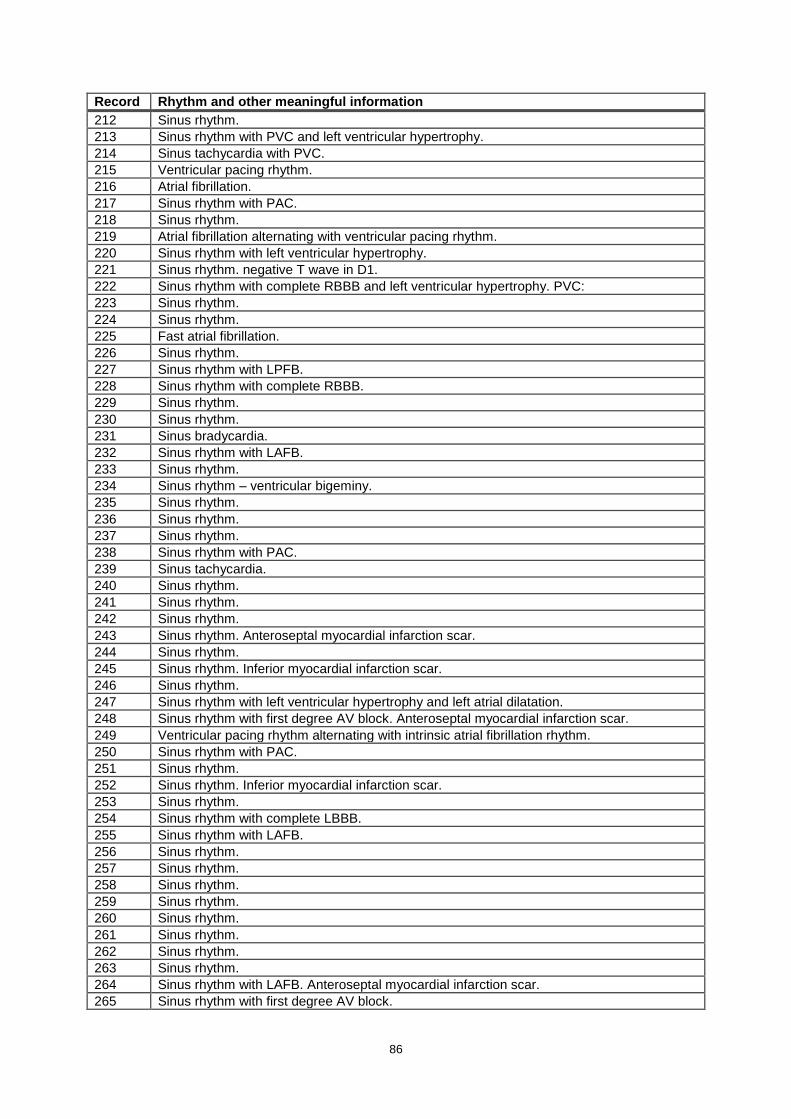
86
Record Rhythm and other meaningful information
212 Sinus rhythm.
213 Sinus rhythm with PVC and left ventricular hypertrophy.
214 Sinus tachycardia with PVC.
215 Ventricular pacing rhythm.
216 Atrial fibrillation.
217 Sinus rhythm with PAC.
218 Sinus rhythm.
219 Atrial fibrillation alternating with ventricular pacing rhythm.
220 Sinus rhythm with left ventricular hypertrophy.
221 Sinus rhythm. negative T wave in D1.
222 Sinus rhythm with complete RBBB and left ventricular hypertrophy. PVC:
223 Sinus rhythm.
224 Sinus rhythm.
225 Fast atrial fibrillation.
226 Sinus rhythm.
227 Sinus rhythm with LPFB.
228 Sinus rhythm with complete RBBB.
229 Sinus rhythm.
230 Sinus rhythm.
231 Sinus bradycardia.
232 Sinus rhythm with LAFB.
233 Sinus rhythm.
234 Sinus rhythm – ventricular bigeminy.
235 Sinus rhythm.
236 Sinus rhythm.
237 Sinus rhythm.
238 Sinus rhythm with PAC.
239 Sinus tachycardia.
240 Sinus rhythm.
241 Sinus rhythm.
242 Sinus rhythm.
243 Sinus rhythm. Anteroseptal myocardial infarction scar.
244 Sinus rhythm.
245 Sinus rhythm. Inferior myocardial infarction scar.
246 Sinus rhythm.
247 Sinus rhythm with left ventricular hypertrophy and left atrial dilatation.
248 Sinus rhythm with first degree AV block. Anteroseptal myocardial infarction scar.
249 Ventricular pacing rhythm alternating with intrinsic atrial fibrillation rhythm.
250 Sinus rhythm with PAC.
251 Sinus rhythm.
252 Sinus rhythm. Inferior myocardial infarction scar.
253 Sinus rhythm.
254 Sinus rhythm with complete LBBB.
255 Sinus rhythm with LAFB.
256 Sinus rhythm.
257 Sinus rhythm.
258 Sinus rhythm.
259 Sinus rhythm.
260 Sinus rhythm.
261 Sinus rhythm.
262 Sinus rhythm.
263 Sinus rhythm.
264 Sinus rhythm with LAFB. Anteroseptal myocardial infarction scar.
265 Sinus rhythm with first degree AV block.

87
Record Rhythm and other meaningful information
266 Sinus rhythm.
267 Sinus rhythm. Switched electrodes.
268 Sinus rhythm.
269 Ventricular pacing rhythm. Atrial fibrillation.
270 Sinus rhythm with first degree AV block.
271 Sinus rhythm with LAFB. Anteroseptal myocardial infarction scar.
272 Sinus rhythm.
273 Sinus rhythm.
274 Sinus rhythm with complete RBBB.
275 Sinus rhythm.
276 Sinus rhythm.
277 Sinus rhythm.
278 Sinus rhythm.
279 Sinus bradycardia. Left ventricular hypertrophy criteria. Negative T wave in D1.
280 Sinus rhythm.
281 Sinus rhythm.
282 Sinus rhythm. PVC and PAC.
283 Sinus rhythm with complete RBBB. left ventricular hypertrophy.
284 Atrial fibrillation with PVC.
285 Atrial fibrillation.
286 Sinus rhythm.
287 Sinus rhythm with left ventricular hypertrophy.
288 Sinus rhythm.
289 Atrial fibrillation.
290 Sinus rhythm with intraventricular conduction aberrancy.
291 Sinus rhythm. Inferior myocardial infarction scar.
292 Sinus rhythm.
293 Sinus rhythm with anteroseptal myocardial infarction scar.
294 Sinus rhythm with complete RBBB.