automatic control and mixed sensitivity hinf control
TRANSCRIPT

Contents Automatic control Background Mixed Sensitivity Benchmark of a Mechanical System Conclusions
Automatic control and mixed sensitivityH∞
control
René Galindo Orozco
FIME - UANL
CINVESTAV-Monterrey, 20 de Febrero de 2008
Contents Automatic control Background Mixed Sensitivity Benchmark of a Mechanical System Conclusions
Contents
1 Automatic control1 Basic notions2 Degree of mechanization3 History4 Class of systems
2 Mixed sensitivityH∞ control1 Motivation2 Basic notions3 Background4 Loop-shaping5 Mixed sensitivity6 Standard solutions7 Parity interlacing property
1 Mixed sensitivityH∞ control in anon conventional scheme
1 A mixed sensitivity problem2 Direct solutions3 Controllers4 Tuning procedure5 Benchmark of a mechanical
system6 Conclusions

Contents Automatic control Background Mixed Sensitivity Benchmark of a Mechanical System Conclusions
Basic notions
Automatic control [Wikipedia]
A research area and theoretical base for mechanization andautomation , employing methods from mathematics andengineering
Theory that deals with influencing the behavior of dynamicsystems
MechanizationMachinery to assist human operators with the physicalrequirements
Automation (ancient Greek: = self dictated) [Salvatencyclopedia]Control systems for industrial machinery andprocesses, replacing human operatorsReduces the need for human sensory and mentalrequirements
Contents Automatic control Background Mixed Sensitivity Benchmark of a Mechanical System Conclusions
Basic notions
Automatic control [Wikipedia]
A research area and theoretical base for mechanization andautomation , employing methods from mathematics andengineeringTheory that deals with influencing the behavior of dynamicsystems
MechanizationMachinery to assist human operators with the physicalrequirements
Automation (ancient Greek: = self dictated) [Salvatencyclopedia]Control systems for industrial machinery andprocesses, replacing human operatorsReduces the need for human sensory and mentalrequirements
Contents Automatic control Background Mixed Sensitivity Benchmark of a Mechanical System Conclusions
Basic notions
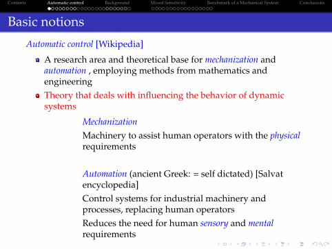
Components [Wikipedia]
u (t) -
f (�)
O& O �O%#&O"
O"
-y (t)
?
d (t)
System , set of interactingentities, real or abstract,forming an integrated whole
Sensor , measure some physical stateController , manipulates u (t) to obtain the desired y (t)Actuator effect a response under the command of the controllerReference or set point , a desired y (t)
Contents Automatic control Background Mixed Sensitivity Benchmark of a Mechanical System Conclusions
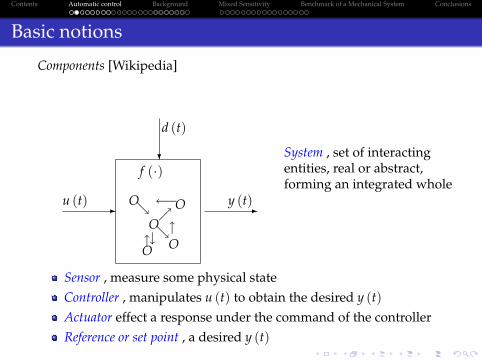
Controller improved by J. Watt
Contents Automatic control Background Mixed Sensitivity Benchmark of a Mechanical System Conclusions
Basic notions
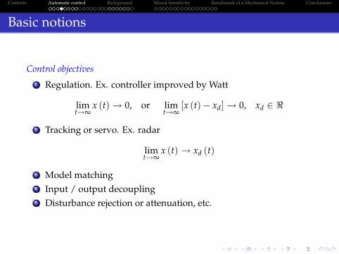
Control objectives1 Regulation. Ex. controller improved by Watt
limt!∞
x (t)! 0, or limt!∞
[x (t)� xd]! 0, xd 2 <
2 Tracking or servo. Ex. radar
limt!∞
x (t)! xd (t)
3 Model matching4 Input / output decoupling5 Disturbance rejection or attenuation, etc.
Contents Automatic control Background Mixed Sensitivity Benchmark of a Mechanical System Conclusions
Basic notions
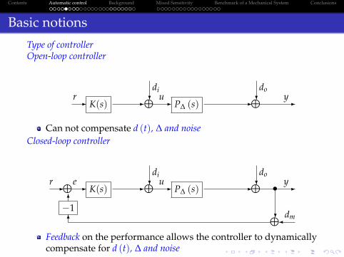
Type of controllerOpen-loop controller
-r K(s) -Ldi?u- P∆ (s) -Ldo
? -y
Can not compensate d (t), ∆ and noiseClosed-loop controller
r-L -e K(s) -Ldi?u- P∆ (s) -Ldo
? -� y
?L dm�6�16
Feedback on the performance allows the controller to dynamicallycompensate for d (t), ∆ and noise
Contents Automatic control Background Mixed Sensitivity Benchmark of a Mechanical System Conclusions
Basic notions
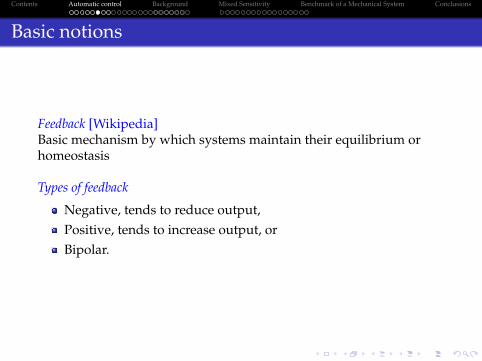
Feedback [Wikipedia]Basic mechanism by which systems maintain their equilibrium orhomeostasis
Types of feedback
Negative, tends to reduce output,Positive, tends to increase output, orBipolar.
Contents Automatic control Background Mixed Sensitivity Benchmark of a Mechanical System Conclusions
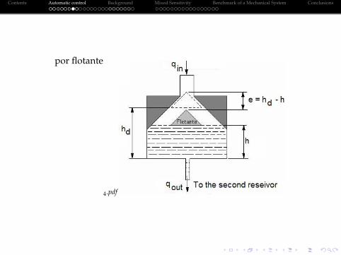
por flotante
4.pdf
Contents Automatic control Background Mixed Sensitivity Benchmark of a Mechanical System Conclusions
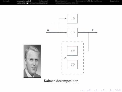
Kalman decomposition

Contents Automatic control Background Mixed Sensitivity Benchmark of a Mechanical System Conclusions
Degree of mechanization
[Salvat encyclopedia]
Contents Automatic control Background Mixed Sensitivity Benchmark of a Mechanical System Conclusions
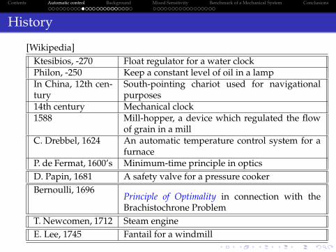
History
[Wikipedia]Ktesibios, -270 Float regulator for a water clockPhilon, -250 Keep a constant level of oil in a lampIn China, 12th cen-tury
South-pointing chariot used for navigationalpurposes
14th century Mechanical clock1588 Mill-hopper, a device which regulated the flow
of grain in a millC. Drebbel, 1624 An automatic temperature control system for a
furnaceP. de Fermat, 1600’s Minimum-time principle in opticsD. Papin, 1681 A safety valve for a pressure cookerBernoulli, 1696
Principle of Optimality in connection with theBrachistochrone Problem
T. Newcomen, 1712 Steam engineE. Lee, 1745 Fantail for a windmill
Contents Automatic control Background Mixed Sensitivity Benchmark of a Mechanical System Conclusions
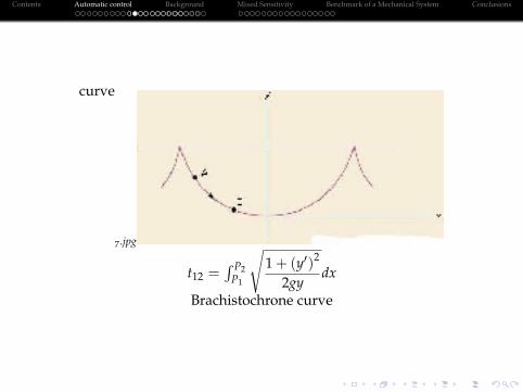
curve
7.jpg
t12 =R P2
P1
s1+ (y0)2
2gydx
Brachistochrone curve
Contents Automatic control Background Mixed Sensitivity Benchmark of a Mechanical System Conclusions
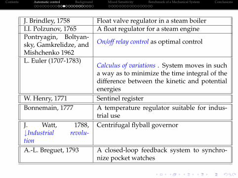
J. Brindley, 1758 Float valve regulator in a steam boilerI.I. Polzunov, 1765 A float regulator for a steam enginePontryagin, Boltyan-sky, Gamkrelidze, andMishchenko 1962
On/off relay control as optimal control
L. Euler (1707-1783)Calculus of variations . System moves in sucha way as to minimize the time integral of thedifference between the kinetic and potentialenergies
W. Henry, 1771 Sentinel registerBonnemain, 1777 A temperature regulator suitable for indus-
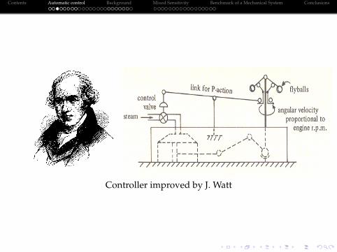
trial useJ. Watt, 1788,#Industrial revolu-tion
Centrifugal flyball governor
A.-L. Breguet, 1793 A closed-loop feedback system to synchro-nize pocket watches

Contents Automatic control Background Mixed Sensitivity Benchmark of a Mechanical System Conclusions
R. Delap, M. Murray, 1799 Pressure regulatorBoulton, Watt, 1803 Combined a pressure regulator with a
float regulatorI. Newton (1642-1727),G.W. Leibniz (1646-1716),brothers Bernoulli (late1600’s, early 1700’s), J.F.Riccati (1676-1754)
Infinitesimal calculus
G.B. Airy, 1840 A feedback device for pointing a tele-scope. Discuss the instability of closed-loopsystems . Analysis using differential equa-tions
J.L. Lagrange (1736-1813), W.R. Hamilton(1805-1865)
Motion of dynamical systems using differ-ential equations
C. Babbage, 1830 Computer principlesJ.C. Maxwell, 1868, I.I.Vishnegradsky, 1877,"Prehistory
Analyzed the stability of Watt’s flyballgovernor, Re froots (G (s))g < 0
Contents Automatic control Background Mixed Sensitivity Benchmark of a Mechanical System Conclusions
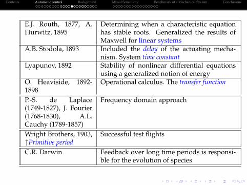
E.J. Routh, 1877, A.Hurwitz, 1895
Determining when a characteristic equationhas stable roots. Generalized the results ofMaxwell for linear systems
A.B. Stodola, 1893 Included the delay of the actuating mecha-nism. System time constant
Lyapunov, 1892 Stability of nonlinear differential equationsusing a generalized notion of energy
O. Heaviside, 1892-1898
Operational calculus. The transfer function
P.-S. de Laplace(1749-1827), J. Fourier(1768-1830), A.L.Cauchy (1789-1857)
Frequency domain approach
Wright Brothers, 1903,"Primitive period
Successful test flights
C.R. Darwin Feedback over long time periods is responsi-ble for the evolution of species
Contents Automatic control Background Mixed Sensitivity Benchmark of a Mechanical System Conclusions
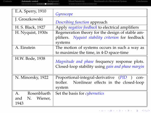
E.A. Sperry, 1910Gyroscope
J. GroszkowskiDescribing function approach
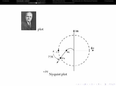
H. S. Black, 1927 Apply negative feedback to electrical amplifiersH. Nyquist, 1930s Regeneration theory for the design of stable am-
plifiers. Nyquist stability criterion for feedbacksystems
A. Einstein The motion of systems occurs in such a way asto maximize the time, in 4-D space-time
H.W. Bode, 1938Magnitude and phase frequency response plots.Closed-loop stability using gain and phase margin
N. Minorsky, 1922 Proportional-integral-derivative (PID ) con-troller. Nonlinear effects in the closed-loopsystem
A. Rosenbluethand N. Wiener,1943
Set the basis for cybernetics
Contents Automatic control Background Mixed Sensitivity Benchmark of a Mechanical System Conclusions
plot
9.jpgNyquist plot

Contents Automatic control Background Mixed Sensitivity Benchmark of a Mechanical System Conclusions
V. Volterra, 1931 Explained the balance between two populationsof fish using feedback
H.L. Házen, 1934 Theory of ServomechanismsA.N. Kolmogorov,1941
Theory for discrete-time stationary stochasticprocesses
N. Wiener, 1942 Statistically optimal filter for stationarycontinuous-time signals
A.C. Hall, 1946 Confront noise effects in frequency-domainN.B. Nichols, 1947
Nichols ChartIvachenko, 1948
Relay controlW.R. Evans, 1948
Root locus techniqueJ. R. Ragazzini,1950s Digital control and the z-transform
Tsypkin, 1955 Phase plane for nonlinear controls

Contents Automatic control Background Mixed Sensitivity Benchmark of a Mechanical System Conclusions
J. von Neumann, 1948 Construction of the IAS stored-programSperry Rand, 1950 Commercial data processing machine, UNI-
VAC IR. Bellman, 1957 Dynamic programming to the optimal con-
trol of discrete-time systemsL.S. Pontryagin, 1958 Maximum principleC.S. Draper, 1960,"Classical period#Modern period
Inertial navigation system
V.M. Popov, 1961Circle criterion for nonlinear stability analysis
Kalman, 1960’s Linear quadratic regulator (LQR ). Discreteand continuous Kalman filter . Linear algebraand matrices. Internal system state
G. Zames, 1966, I.W.Sandberg, K.S. Naren-dra, Goldwyn, 1964,C.A. Desoer, 1965
Nonlinear stability
Contents Automatic control Background Mixed Sensitivity Benchmark of a Mechanical System Conclusions
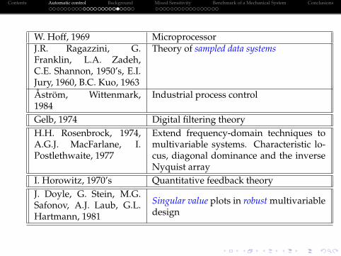
W. Hoff, 1969 MicroprocessorJ.R. Ragazzini, G.Franklin, L.A. Zadeh,C.E. Shannon, 1950’s, E.I.Jury, 1960, B.C. Kuo, 1963
Theory of sampled data systems
Åström, Wittenmark,1984
Industrial process control
Gelb, 1974 Digital filtering theoryH.H. Rosenbrock, 1974,A.G.J. MacFarlane, I.Postlethwaite, 1977
Extend frequency-domain techniques tomultivariable systems. Characteristic lo-cus, diagonal dominance and the inverseNyquist array
I. Horowitz, 1970’s Quantitative feedback theoryJ. Doyle, G. Stein, M.G.Safonov, A.J. Laub, G.L.Hartmann, 1981
Singular value plots in robust multivariabledesign
Contents Automatic control Background Mixed Sensitivity Benchmark of a Mechanical System Conclusions
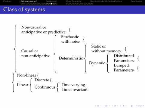
Class of systems
8>>>>>>>>>>>>>><>>>>>>>>>>>>>>:
Non-causal oranticipative or predictive f
Causal ornon-anticipative
8>>>>>>>>>><>>>>>>>>>>:
Stochasticwith noise f
Deterministic
8>>>>>><>>>>>>:
Static orwithout memory f
Dynamic
8>><>>:DistributedParameters fLumpedParameters f8>><>>:
Non-linear f
Linear
8<: Discrete fContinuous
�Time varyingTime invariant

Contents Automatic control Background Mixed Sensitivity Benchmark of a Mechanical System Conclusions
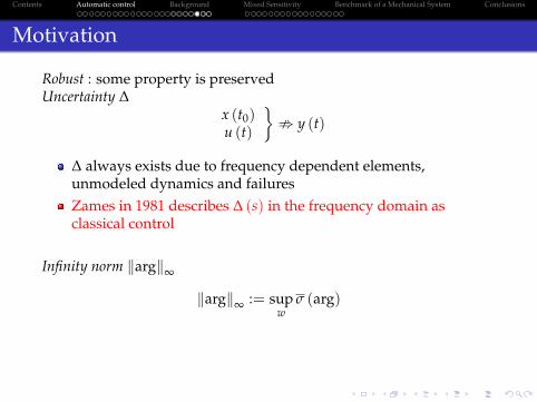
Motivation
Robust : some property is preservedUncertainty ∆
x (t0)u (t)
�; y (t)
∆ always exists due to frequency dependent elements,unmodeled dynamics and failures
Zames in 1981 describes ∆ (s) in the frequency domain asclassical control
Infinity norm kargk∞
kargk∞ := supw
σ (arg)
kargk∞ is “good” for specifying the ∆ level and the effect ofkd (t)k2 < ∞ over ky (t)k2
Contents Automatic control Background Mixed Sensitivity Benchmark of a Mechanical System Conclusions
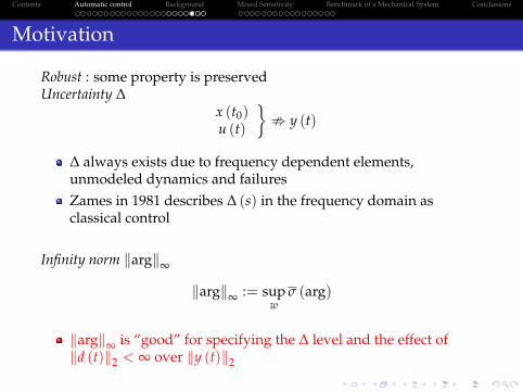
Motivation
Robust : some property is preservedUncertainty ∆
x (t0)u (t)
�; y (t)
∆ always exists due to frequency dependent elements,unmodeled dynamics and failuresZames in 1981 describes ∆ (s) in the frequency domain asclassical control
Infinity norm kargk∞
kargk∞ := supw
σ (arg)
kargk∞ is “good” for specifying the ∆ level and the effect ofkd (t)k2 < ∞ over ky (t)k2
Contents Automatic control Background Mixed Sensitivity Benchmark of a Mechanical System Conclusions
Motivation
Robust : some property is preservedUncertainty ∆
x (t0)u (t)
�; y (t)
∆ always exists due to frequency dependent elements,unmodeled dynamics and failuresZames in 1981 describes ∆ (s) in the frequency domain asclassical control
Infinity norm kargk∞
kargk∞ := supw
σ (arg)
kargk∞ is “good” for specifying the ∆ level and the effect ofkd (t)k2 < ∞ over ky (t)k2

Contents Automatic control Background Mixed Sensitivity Benchmark of a Mechanical System Conclusions
Basic notions
RobustH∞ control objective
r�L�eK(s)
-
w- G (s)z-
- e∆ (s)�
?�1?
Uncertainty and kw (t)k2 attenuationin a bandwidth, over kz (t)k2,guaranteeing stability
Minimize,
J := kz (t)k2 :=�Z ∞
�∞z2 (t) dt
�1/2
For linear time invariant systems, minimizeJ := kTzew (s)k∞ := supew(t):kew(t)k2�1 σ (Tzew), or J := σ (Tzew (s))
Contents Automatic control Background Mixed Sensitivity Benchmark of a Mechanical System Conclusions
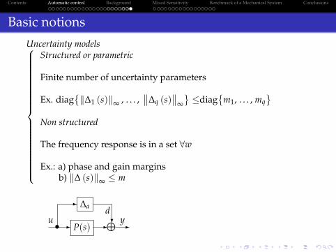
Basic notions
Uncertainty models8>>>>>>>>>>>>>>>>>><>>>>>>>>>>>>>>>>>>:
Structured or parametric
Finite number of uncertainty parameters
Ex. diag�k∆1 (s)k∞ , . . . ,
∆q (s)
∞
�diag
�m1, . . . , mq
Non structured
The frequency response is in a set 8w
Ex.: a) phase and gain marginsb) k∆ (s)k∞ � m
u - P(s) -L -yd?�
- ∆a
Figure:

Contents Automatic control Background Mixed Sensitivity Benchmark of a Mechanical System Conclusions
D.C. Youla, H. A.Jabr, J.J. Bongiorno;1976
Explicit formula for the optimal controller basedon a least-square Wiener-Hopf minimization of acost functional
C.A. Desoer, R. Liu,J. Murray, R. Saeks;1980
Controllers placing the feedback system in a ringof operators with the prescribed properties. Theplant is modeled as a ratio of two operators in thatring
M. Vidyasagar, H.Schneider, B.A.Francis, 1982
Necessary and sufficient conditions for a giventransfer function matrix to have a coprime factor-ization . Characterization of all stabilizing compen-sators
C.N. Nett, C.A. Ja-cobson, M. J. Balas;1984
Give explicit formulas for a doubly coprime frac-tional representation of the transfer function instate-space
K. Glover, D. Mc-Farlane, 1989
An optimal stability margin. Characterizationof all controllers satisfying a suboptimal stabil-ity margin, in state-space
Contents Automatic control Background Mixed Sensitivity Benchmark of a Mechanical System Conclusions
Loop-shaping
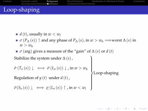
d (t), usually in w < wl
σ (P∆ (s)) " and any phase of P∆ (s), in w > wh =)worst ∆ (s) inw > wh
σ (arg) gives a measure of the “gain” of ∆ (s) or d (t)
Stabilize the system under ∆ (s) ,
σ (To (s)) # ()_σ (Lo (s)) # , in w > wh
Regulation of y (t) under d (t) ,
_σ(So (s)) # () σ (Lo (s)) " , in w < wl
9>>>>>>>>=>>>>>>>>;Loop-shaping
Contents Automatic control Background Mixed Sensitivity Benchmark of a Mechanical System Conclusions
Loop-shaping
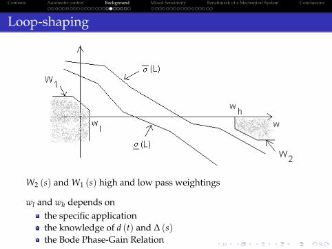
W2 (s) and W1 (s) high and low pass weightings
wl and wh depends onthe specific applicationthe knowledge of d (t) and ∆ (s)the Bode Phase-Gain Relation
Contents Automatic control Background Mixed Sensitivity Benchmark of a Mechanical System Conclusions
Mixed sensitivity
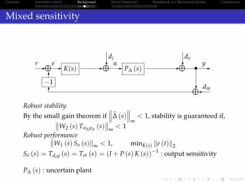
r-L -e K(s) -Ldi?u- P∆ (s) -Ldo
? -� y
?L dm�6�16
Robust stabilityBy the small gain theorem if
e∆ (s) ∞< 1, stability is guaranteed if, W2 (s)Tu∆y∆ (s)
∞ < 1
Robust performancekW1 (s) So (s)k∞ < 1, minK(s) ke (t)k2
So (s) = Tdoy (s) = Ter (s) = (I+ P (s)K (s))�1 : output sensitivity
P∆ (s) : uncertain plant
Contents Automatic control Background Mixed Sensitivity Benchmark of a Mechanical System Conclusions
Mixed sensitivity
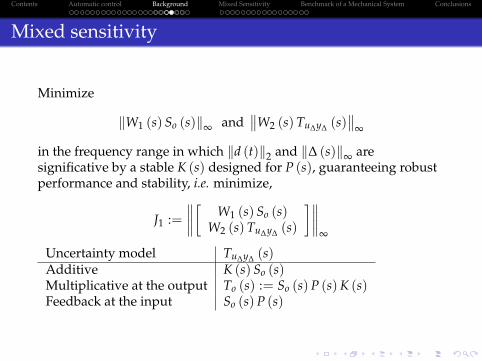
Minimize
kW1 (s) So (s)k∞ and W2 (s)Tu∆y∆ (s)
∞
in the frequency range in which kd (t)k2 and k∆ (s)k∞ aresignificative by a stable K (s) designed for P (s), guaranteeing robustperformance and stability, i.e. minimize,
J1 := � W1 (s) So (s)
W2 (s)Tu∆y∆ (s)
� ∞
Uncertainty model Tu∆y∆ (s)Additive K (s) So (s)Multiplicative at the output To (s) := So (s)P (s)K (s)Feedback at the input So (s)P (s)
Contents Automatic control Background Mixed Sensitivity Benchmark of a Mechanical System Conclusions
Standard solutions
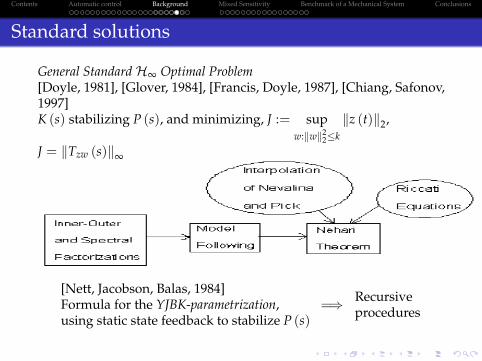
General StandardH∞ Optimal Problem[Doyle, 1981], [Glover, 1984], [Francis, Doyle, 1987], [Chiang, Safonov,1997]K (s) stabilizing P (s), and minimizing, J := sup
w:kwk22�k
kz (t)k2,
J = kTzw (s)k∞
[Nett, Jacobson, Balas, 1984]Formula for the YJBK-parametrization,using static state feedback to stabilize P (s)
=) Recursiveprocedures
Contents Automatic control Background Mixed Sensitivity Benchmark of a Mechanical System Conclusions
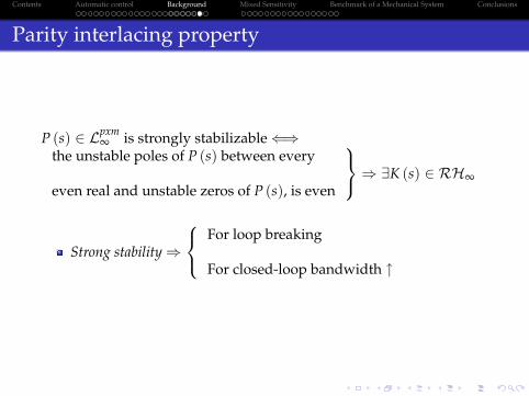
Parity interlacing property
P (s) 2 Lpxm∞ is strongly stabilizable()
the unstable poles of P (s) between every
even real and unstable zeros of P (s), is even
9=;) 9K (s) 2 RH∞
Strong stability)
8<: For loop breaking
For closed-loop bandwidth "
Contents Automatic control Background Mixed Sensitivity Benchmark of a Mechanical System Conclusions
Problem
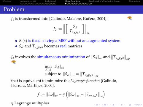
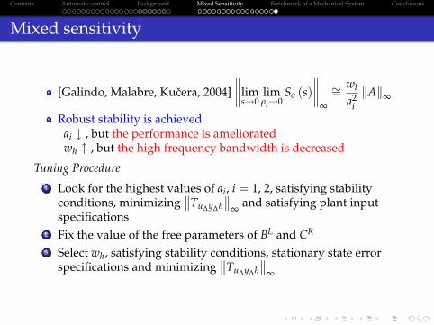
J1 is transformed into [Galindo, Malabre, Kucera, 2004]:
J2 := � Sol
Tu∆y∆h
� ∞
R (s) is fixed solving a MSP without an augmented systemSol and Tu∆y∆h becomes real matrices
J2 involves the simultaneous minimization of kSolk∞ and Tu∆y∆h
∞,
minK(s)kSolk∞
subject to kSolk∞ = Tu∆y∆h
∞
that is equivalent to minimize the Lagrange function [Galindo,Herrera, Martínez, 2000],
f := kSolk∞ � η�kSolk∞ �
Tu∆y∆h
∞
�η Lagrange multiplier
Contents Automatic control Background Mixed Sensitivity Benchmark of a Mechanical System Conclusions
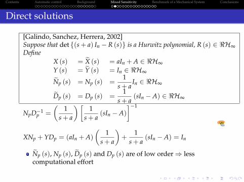
Direct solutions
[Galindo, Sanchez, Herrera, 2002]Suppose that det f(s+ a) In � R (s)g is a Hurwitz polynomial, R (s) 2 <H∞Define
X (s) = eX (s) = aIn +A 2 <H∞Y (s) = eY (s) = In 2 <H∞eNp (s) = Np (s) =
1s+ a
In 2 <H∞eDp (s) = Dp (s) =1
s+ a(sIn �A) 2 <H∞
NpD�1p =
�1
s+ a
� �1
s+ a(sIn �A)
��1
XNp + YDp = (aIn +A)�
1s+ a
�+
1s+ a
(sIn �A) = In
eNp (s), Np (s), eDp (s) and Dp (s) are of low order) lesscomputational effort
Contents Automatic control Background Mixed Sensitivity Benchmark of a Mechanical System Conclusions
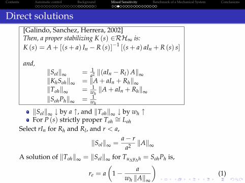
Direct solutions[Galindo, Sanchez, Herrera, 2002]Then, a proper stabilizing K (s) 2RH∞ is:K (s) = A+ [(s+ a) In � R (s)]�1 [(s+ a) aIn + R (s) s]
and,kSolk∞ = 1
a2 k(aIn � Rl)Ak∞kKhSohk∞ = kA+ aIn + Rhk∞kTohk∞ = 1
whkA+ aIn + Rhk∞
kSohPhk∞ = 1wh
kSolk∞ # by a ", and kTohk∞ # by wh "For P (s) strictly proper Toh
�= LohSelect rIn for Rh and Rl, and r < a,
kSolk∞ =a� r
a2 kAk∞
A solution of kTohk∞ = kSolk∞ for Tu∆y∆h = SohPh is,
re = a�
1� awh kAk∞
�(1)
implying kSolk∞ = 1/wh, and J2 is satisfied increasing wh
Contents Automatic control Background Mixed Sensitivity Benchmark of a Mechanical System Conclusions
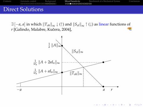
Direct Solutions
9 [�a, a] in which kTohk∞ # (") and kSolk∞ " (#) as linear functions ofr [Galindo, Malabre, Kucera, 2004],
-�a
������
������
������
������
6
1whkA+ aInk∞ �
1whkA+ 2aInk∞ �
1a kAk∞�
@@
@@
@@
@@
@@
@@
�a r
kSolk∞
kTohk∞
Contents Automatic control Background Mixed Sensitivity Benchmark of a Mechanical System Conclusions
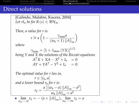
Direct solutions[Galindo, Malabre, Kucera, 2004]Let rIn be for R (s) 2 <H∞
Then, a value for r is:
r �= a�
1� γmina(wh + 1) kAk∞
�where
γmin = [1+ λmax (YX)]1/2
being Y and X the solutions of the Riccati equationsATX+XA�X2 + In = 0AY+ YAT � Y2 + In = 0
The optimal value for r lies in,r 2 [rb, a]
and a lower bound rb for r is:
rb =a�(wh � a) kAk∞ � a2�
wh kAk∞ + a2
limwh�!0
rb = � (a+ kAk∞), limwh�!∞
rb = a

Contents Automatic control Background Mixed Sensitivity Benchmark of a Mechanical System Conclusions
Let rIn be for R (s) 2 <H∞
Then, an optimal value for r is:
re =b2 � b1
m1 �m2where
b1 :=1akAk∞ , m1 :=
�1a2 kAk∞
b2 :=1
whkA+ aInk∞
m2 :=1
awh(kA+ 2aInk∞ � kA+ aInk∞)
Moreover
kSolk∞ =kA+ 2aInk∞ kAk∞
wh kAk∞ + a (kA+ 2aInk∞ � kA+ aInk∞)

Contents Automatic control Background Mixed Sensitivity Benchmark of a Mechanical System Conclusions
Controllers
x (t) = Ax (t) + Bu (t)Define v1 (t) := Bu (t) ) x (t) = Ax (t) + v1 (t)
+u (t) = BLv1 (t) ) x (t) = Ax (t) + BBLv1 (t)
) E1 := BBL � In
xd-L - K1(s)v1- BL -u
(sIn �A)�1 B -Ld1? -� x
?L d2�6�16
A 2 <n�n, B 2 <n�m, C 2 <p�n
v1 (t) the output of the precompensator K1 (s)BL a left inverse of Bxd (t) the input reference
Contents Automatic control Background Mixed Sensitivity Benchmark of a Mechanical System Conclusions
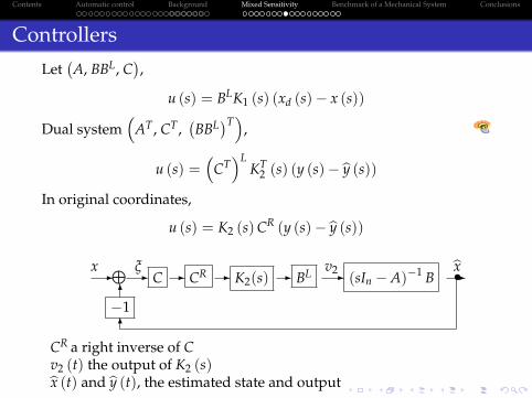
Controllers
Let�A, BBL, C
�,
u (s) = BLK1 (s) (xd (s)� x (s))
Dual system�
AT, CT,�BBL�T
�,
u (s) =�
CT�L
KT2 (s) (y (s)� by (s))
In original coordinates,
u (s) = K2 (s)CR (y (s)� by (s))x-L ξ- C - CR - K2(s) - BL -v2
(sIn �A)�1 B -�bx6�16
CR a right inverse of Cv2 (t) the output of K2 (s)bx (t) and by (t), the estimated state and output
Contents Automatic control Background Mixed Sensitivity Benchmark of a Mechanical System Conclusions
Controllers
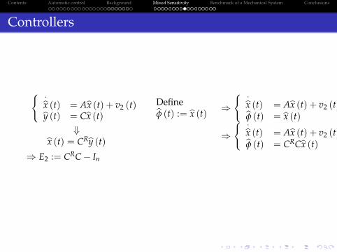
( �bx (t) = Abx (t) + v2 (t)by (t) = Cbx (t) Definebφ (t) := bx (t) )( �bx (t) = Abx (t) + v2 (t)bφ (t) = bx (t)
+bx (t) = CRby (t) )( �bx (t) = Abx (t) + v2 (t)bφ (t) = CRCbx (t)
) E2 := CRC� In
Contents Automatic control Background Mixed Sensitivity Benchmark of a Mechanical System Conclusions
Controllers
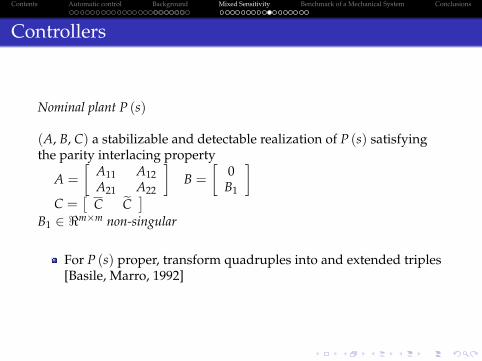
Nominal plant P (s)
(A, B, C) a stabilizable and detectable realization of P (s) satisfyingthe parity interlacing property
A =�
A11 A12A21 A22
�B =
�0
B1
�C =
�C eC �
B1 2 <m�m non-singular
For P (s) proper, transform quadruples into and extended triples[Basile, Marro, 1992]
Contents Automatic control Background Mixed Sensitivity Benchmark of a Mechanical System Conclusions
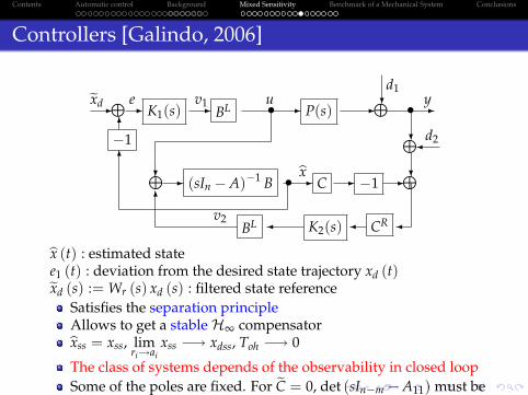
Controllers [Galindo, 2006]
exd-L e- K1(s)v1- BL -�
?
uP(s) -Ld1
? -� y
?L?
d2�6�16
L - (sIn �A)�1 Bbx� - C - �1 -L
�CR�K2(s)v2 �BL
6
bx (t) : estimated statee1 (t) : deviation from the desired state trajectory xd (t)exd (s) := Wr (s) xd (s) : filtered state reference
Satisfies the separation principleAllows to get a stableH∞ compensatorbxss = xss, lim
ri!aixss �! xdss, Toh �! 0
The class of systems depends of the observability in closed loopSome of the poles are fixed. For eC = 0, det (sIn�m �A11) must beHurwitz
Contents Automatic control Background Mixed Sensitivity Benchmark of a Mechanical System Conclusions
Controllers
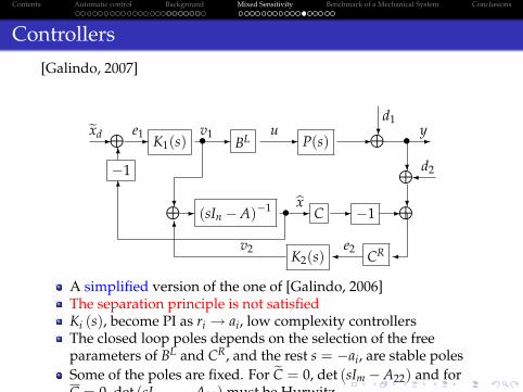
[Galindo, 2007]
exd-L e1- K1(s)v1-�
?
BL -uP(s) -Ld1
? -� y
?L?
d2�6�16
L- (sIn �A)�1 bx� - C - �1 -L�CRe2�K2(s)
v2
6
A simplified version of the one of [Galindo, 2006]The separation principle is not satisfiedKi (s), become PI as ri ! ai, low complexity controllersThe closed loop poles depends on the selection of the freeparameters of BL and CR, and the rest s = �ai, are stable polesSome of the poles are fixed. For eC = 0, det (sIm �A22) and forC = 0, det (sIn�m �A11) must be Hurwitz
Contents Automatic control Background Mixed Sensitivity Benchmark of a Mechanical System Conclusions
Tuning procedure
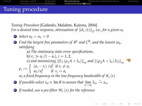
Tuning Procedure [Galindo, Malabre, Kucera, 2004]For a desired time response, attenuation of kd1 (t)k2, i.e., for a given a1
1 Select a2 = a1 > 02 Find the largest free parameters of BL and CR, and the lowest wh,
satisfyinga) The stationary state error specifications,b) ri � ai (1� ai), i = 1, 2,c) and minimizing kE1 (ρ1A+ In)k∞ and k(ρ2A+ In)E2k∞
ρi :=�(ai � ri) /a2
i if ri 6= aiwl/a2
i if ri = aiwl a fixed frequency in the low frequency bandwidth of Ki (s)
3 If possible select xd 2 Im B to assure that limri!ai
bxss�! xss
4 If needed, use a pre-filter Wr (s) for the reference
Contents Automatic control Background Mixed Sensitivity Benchmark of a Mechanical System Conclusions
Controllers
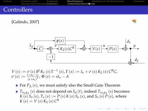
[Galindo, 2007]
exd�
- φ(s)?- C -L e- K2(s)CR -L- V(s) -u P(s) -
Ld1? -� y
?L d2�6�16
V (s) := σ (s)BLK1 (s) Γ�1 (s), Γ (s) := In + σ (s)K2 (s)CRC,σ (s) := s+a1�r1
(s+a1)2 , Φ (s) = sIn �A
For P∆ (s), we must satisfy also the Small Gain TheoremTu∆y∆ (s) does not depend on exd (t), indeed Tu∆y∆ (s) becomesK (s) So (s), To (s) := P (s)K (s) So (s), and So (s)P (s), whereK (s) = V (s)K2 (s)CR
Contents Automatic control Background Mixed Sensitivity Benchmark of a Mechanical System Conclusions
Controllers
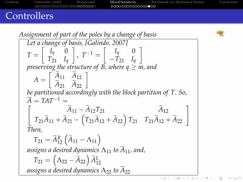
Assignment of part of the poles by a change of basisLet a change of basis, [Galindo, 2007]
T =�
Iq 0T21 Iq
�, T�1 =
�Iq 0�T21 Iq
�preserving the structure of B, where q � m, and
A =� eA11 eA12eA21 eA22
�be partitioned accordingly with the block partition of T. So,A = TAT�1 =" eA11 � eA12T21 eA12
T21eA11 + eA21 ��
T21eA12 + eA22
�T21 T21eA12 + eA22
#Then,
T21 = eAR12
�eA11 �Λ11
�assigns a desired dynamics Λ11 to A11, and,
T21 =�
Λ22 � eA22
� eAL12
assigns a desired dynamics Λ22 to A22
Contents Automatic control Background Mixed Sensitivity Benchmark of a Mechanical System Conclusions
Mixed sensitivity
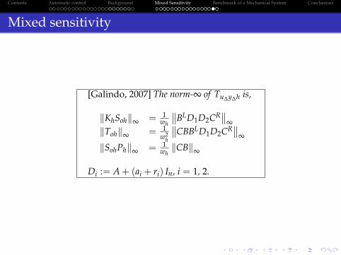
[Galindo, 2007] The norm-∞ of Tu∆y∆h is,
kKhSohk∞ = 1wh
BLD1D2CR
∞kTohk∞ = 1
w2h
CBBLD1D2CR
∞
kSohPhk∞ = 1whkCBk∞
Di := A+ (ai + ri) In, i = 1, 2.
Contents Automatic control Background Mixed Sensitivity Benchmark of a Mechanical System Conclusions
Mixed sensitivity
[Galindo, Malabre, Kucera, 2004] lim
s!0limρi!0
So (s)
∞
�= wl
a2ikAk∞
Robust stability is achievedai # , but the performance is amelioratedwh " , but the high frequency bandwidth is decreased
Tuning Procedure1 Look for the highest values of ai, i = 1, 2, satisfying stability
conditions, minimizing Tu∆y∆h
∞ and satisfying plant input
specifications2 Fix the value of the free parameters of BL and CR
3 Select wh, satisfying stability conditions, stationary state errorspecifications and minimizing
Tu∆y∆h
∞

Contents Automatic control Background Mixed Sensitivity Benchmark of a Mechanical System Conclusions
Benchmark of a Mechanical System
-u
m1
7�! x1(t)
kb
m2
7�! x2(t)
-d
Consider a model of a mechanical system,�x (t) = Ax (t) + Bu (t) +Ψd (t)y (t) = Cx (t)
where x (t)T :=�
x1 (t) x2 (t) x2 (t) x1 (t)�,
A =
266640 0 0 10 0 1 0
km2
�km2
�bm2
bm2
�km1
km1
bm1
�bm1
37775 , B =
2664000
1m1
3775 , Ψ =
2664001
m20
3775C =
�0 1 0 0
�
Contents Automatic control Background Mixed Sensitivity Benchmark of a Mechanical System Conclusions
Benchmark of a Mechanical System
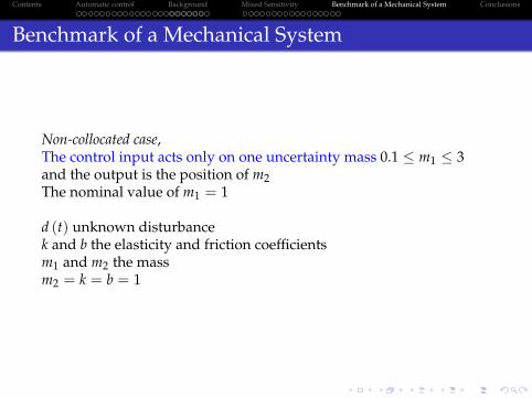
Non-collocated case,The control input acts only on one uncertainty mass 0.1 � m1 � 3and the output is the position of m2The nominal value of m1 = 1
d (t) unknown disturbancek and b the elasticity and friction coefficientsm1 and m2 the massm2 = k = b = 1
Contents Automatic control Background Mixed Sensitivity Benchmark of a Mechanical System Conclusions
Benchmark of a Mechanical System
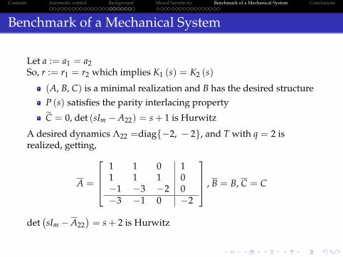
Let a := a1 = a2So, r := r1 = r2 which implies K1 (s) = K2 (s)
(A, B, C) is a minimal realization and B has the desired structureP (s) satisfies the parity interlacing propertyeC = 0, det (sIm �A22) = s+ 1 is Hurwitz
A desired dynamics Λ22 =diagf�2, � 2g, and T with q = 2 isrealized, getting,
A =
26641 1 0 11 1 1 0�1 �3 �2 0�3 �1 0 �2
3775 , B = B, C = C
det�sIm �A22
�= s+ 2 is Hurwitz

Contents Automatic control Background Mixed Sensitivity Benchmark of a Mechanical System Conclusions
Benchmark of a Mechanical System
Select a = 2 and,
BL =�
g1 0 0 1�
CR =�
g2 1 0 g3�T
g1 = 1.6, g2 = 0.3, g3 = �0.55
CB = 0 =) kTohk∞ = 0 and kSohPhk∞ = 0,
wh kKhSohk∞ kKhSohk∞ kKhSohk∞with r with rb with re
1 1.9 stable 0.05 unstable 0.909 unstable3 0.675 stable 0.487 unstable 0.57 unstable5 0.412 unstable 0.35 unstable 0.377 stable10 0.209 unstable 0.195 stable 0.201 stable12 0.175 unstable 0.165 stable 0.169 stable15 0.14 unstable 0.134 stable 0.136 unstable17 0.124 unstable 0.119 stable 0.121 unstable18 0.117 unstable 0.113 stable 0.114 unstable20 0.105 unstable 0.102 unstable 0.103 unstable
Contents Automatic control Background Mixed Sensitivity Benchmark of a Mechanical System Conclusions
Benchmark of a Mechanical System
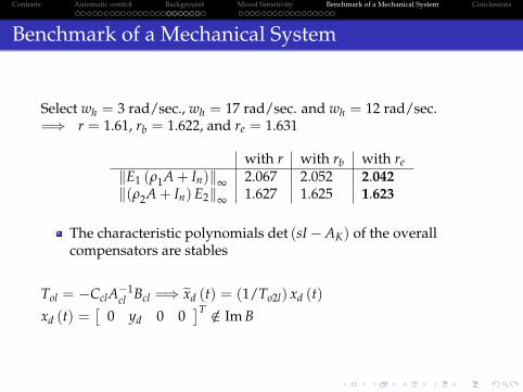
Select wh = 3 rad/sec., wh = 17 rad/sec. and wh = 12 rad/sec.=) r = 1.61, rb = 1.622, and re = 1.631
with r with rb with rekE1 (ρ1A+ In)k∞ 2.067 2.052 2.042k(ρ2A+ In)E2k∞ 1.627 1.625 1.623
The characteristic polynomials det (sI�AK) of the overallcompensators are stables
Tol = �CclA�1cl Bcl =) exd (t) = (1/To2l) xd (t)
xd (t) =�
0 yd 0 0�T /2 Im B
Contents Automatic control Background Mixed Sensitivity Benchmark of a Mechanical System Conclusions
Benchmark of a Mechanical System
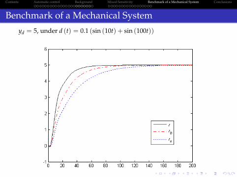
yd = 5, under d (t) = 0.1 (sin (10t) + sin (100t))
Plant output y (t)
Contents Automatic control Background Mixed Sensitivity Benchmark of a Mechanical System Conclusions
Benchmark of a Mechanical System
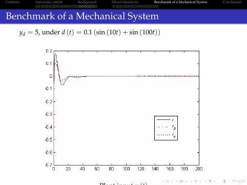
yd = 5, under d (t) = 0.1 (sin (10t) + sin (100t))
Plant input u (t)
Contents Automatic control Background Mixed Sensitivity Benchmark of a Mechanical System Conclusions
Benchmark of a Mechanical System
x2 (t) tracks the reference signal with r, rb and re, under the d (t)and the variation of the parameter m1
d (t) remains as very small oscillations at y (t)Sinusoidal functions of frequencies over wh = 3 rad/sec.,wh = 17 rad/sec. and wh = 12 rad/sec. for r, rb and re, are wellattenuated at y (t)Bigger time response with re and less control energy, the contrarywith r, and rb in the middleSmooth control energyAs m1 ", more energy is required, and the peaks and frequencyof the oscillations decrease
Contents Automatic control Background Mixed Sensitivity Benchmark of a Mechanical System Conclusions
Conclusions
1 A methodology to design a mixed sensitivityH∞ compensatorfor a LTI MIMO plant is proposed
2 A nominal compensator is designed for the nominal plantsolving a mixed sensitivityH∞ problem, in a non-conventionalobserver-compensator scheme
3 A mixed sensitivityH∞ control law and necessary and sufficientstability conditions are given
4 Good performance guaranteeing stability, in spite of theuncertainties and of the external disturbances that are attenuated
5 The controllers with r, rb and re have good performance and theirselection depends on the desired time response and the plantinput specifications
6 An analytic or a numerical method replacing the tuningprocedure is still an open problem

Contents Automatic control Background Mixed Sensitivity Benchmark of a Mechanical System Conclusions
Thank you