automatic control of the heart-lung machine the heart-lung machine ... in this thesis the...
TRANSCRIPT

Automatic Control
of the Heart-Lung Machine
A Dissertation submitted to the
Fakultat fur Elektrotechnik und Informationstechnik
Ruhr-Universitat Bochum
for the degree of Doktor-Ingenieur
Berno Johannes Engelbert Misgeld
Euskirchen, Germany

Dissertation submitted: 27. July, 2006
First examiner: PD Dr. rer. nat. M. Hexamer
Second examiner: Prof. Dr.-Ing. J. Lunze
Oral examination: 16. February, 2007

Kurzfassung
Die vorliegende Arbeit beschreibt die Entwicklung von Regelungsstrategien fur den kardiopul-monalen Bypass mit Unterstutzung der Herz-Lungen-Maschine. Wahrend der Operation amruhenden Herzen ubernimmt die Herz-Lungen-Maschine die Funktion von Herz und Lungeund ermoglicht somit den Eingriff ohne bleibende Schaden fur den Patienten. Hierzu wirddas menschliche Blut dem Korper entnommen, auf kunstlichem Wege mit Sauerstoff angerei-chert und in den Korper zuruckgefuhrt. Obwohl die Herz-Lungen-Maschine uber die letztenJahrzehnte kontinuierlich weiterentwickelt wurde, ist heutzutage noch immer kein geregeltesSystem auf dem Markt erhaltlich. Die Einstellung von wichtigen Vitalvariablen, wie unteranderem Hamodynamik und Blutgase, kann, auch wenn von qualifiziertem Personal vorgenom-men, zu Fehlern fuhren. Dies soll mit der Einfuhrung einer Regelung vermieden werden, um sodas Patientenrisiko zu senken und das behandelnde Personal zu entlasten.Im Hinblick auf eine Regelung von Hamodynamik und Blutgase wurden beide Regelstreckenin detaillierten Modellen in MATLAB/Simulink beschrieben, die teils anhand von Literatur-daten, teils in in-vitro-Experimenten validiert wurden. Anhand dieser Modelle wurden Reglerfur den arteriellen Blutfluss, Blutdruck, Blutfluss mit Blutdruckrandwert und Sauerstoff- bzw.Kohlendioxidpartialdruck entwickelt und eingestellt. Hierbei war die Einstellung der Reglerauf Robustheit bezuglich Nichtlinearitaten, variablen Totzeiten, Artefakten und Parameterun-sicherheiten beim Patienten erforderlich. Alle entwickelten Regler wurden sowohl in Simula-tionen als auch in in-vitro-Experimentalstudien getestet und bewiesen Stabilitat und teils einehohe Gute.Bei der Hamodynamik wurde eine geregelte pulsatile Perfusion in Verbindung mit einer zentrifu-galen Blutpumpe entwickelt. Die arterielle Blutflussregelung war hierbei der Blutdruckregelungdurch die schnelle Einregelzeit und mogliche Ruckflusse, die bei der Blutdruckregelung entste-hen konnen, uberlegen. Die besten Ergebnisse erzielt bei der hamodynamischen Regelung dieBlussflussregelung mit erweiterter Blutdruckrandwertregelung, bei der wahlweise ein stationareroder pulsatiler Modus moglich war. Der arterielle Blutflussregler zeigte das beste Verhalten beiSollwertsprungen oder dem Ausregeln von Druckstorungen.Durch die simultane Regelung der arteriellen Sauerstoff- und Kohlendioxidpartialdrucke konntebei einem gleichzeitig geregelten Blutfluss eine patientengerechte Blutgassituation mit ausrei-chendem Sauerstofffluss ins Gewebe garantiert werden. Die entwickelten Regler reagierten hier-bei mit ausreichender Gute auf Sollwertsprunge. Sowohl in Simulationen als auch im in-vitro-Experiment konnten die Vorgaben bei der Blutgas-Storgroßenregelung unter sich anderndemBlutfluss eingehalten werden.Im Hinblick auf die weitere Validierung im Tierexperiment sowie eine Validierung in zukunf-tigen klinischen Tests konnte ein umfassendes Regelungskonzept fur die Automatisierung derHerz- und Lungenfunktion entwickelt werden, das auf Basis von detaillierter Systemmodel-lierung entworfen und sowohl in Simulationen als auch im in-vitro-Experiment getestet wurde.

Abstract
In this thesis the development of control strategies for cardiopulmonary bypass with heart-lungmachine support is described. During the surgery on the resting heart, the heart-lung machinetakes over the work of heart and lung. To prevent permanent damage to the patient, theblood is withdrawn from the human body, artificially oxygenated and reperfused. Althoughthe heart-lung machine was further developed and improved over the last decades, no appa-ratus with a feedback control strategy is yet commercially available. Therefore, experiencedperfusionist staff is needed, who continually monitor and adjust the important vital variables,like haemodynamics and blood-gases. With the introduction of automatic control for thesevariables errors are to be avoided, thereby increasing patient’s safety and removing workloadfrom the perfusion technician and the anaesthetist.Regarding the control of haemodynamics and blood-gases, the processes for both plants weremodelled in a detailed approach in MATLAB/Simulink. The developed models were then val-idated in parts in experiments and with literature data. With use of these models, controllersfor arterial blood-flow, blood-pressure, blood-flow with augmented pressure boundary valueand oxygen- and carbon dioxide partial pressures were developed and tuned. The controllerswere thereby robustly tuned with regard to nonlinearities, variable time-delays, artifacts andpatient parameter uncertainties. All of the developed controllers were tested in simulations andin in-vitro experimental test series.For haemodynamics a feedback controlled pulsatile perfusion was developed for a rotary bloodpump. During simulations and measurements, the arterial blood-flow control was superior to thearterial pressure control. This was because of the fast control response time with the blood-flowcontrol and the possible backflows with the pressure control. The best results for haemodynamiccontrol were achieved with the arterial blood-flow control with augmented pressure boundarycontrol, with the option for stationary or pulsatile control. The arterial blood-flow controlshowed the best results concerning fast control reference tracking or disturbance rejection.A proper blood-gas situation with an appropriate oxygen flow to the tissues could be achieved bysimultaneous control of oxygen and carbon dioxide partial pressures. The controllers showed asufficiently fast control reference tracking. The guidelines for disturbance rejection, at a chang-ing blood-flow, could be successfully maintained in simulations and in in-vitro experiments.With regard to a further application in animal experiments and in clinical test series a broadstrategy for the automatic control of heart and lung functions could be developed. This con-trol strategy was designed on the basis of extensive system modelling and was validated insimulations and in in-vitro experiments.

Acknowledgements
This thesis is the result of my work as a research associate at the Department for BiomedicalEngineering, Ruhr-University Bochum, from 2004 to 2006. The interaction with many people,whether physicians, natural scientists or engineers contributed to the achievement.
I would like to express my gratitude first of all to my supervisor Dr. rer. nat. M. Hexamer forproviding me with constant encouragement and support. I greatly appreciated his enthusiasmand benefited from his expert knowledge.
I am also very much indebted to the head of the Biomedical Engineering Department, Prof.Dr.-Ing. J. Werner for his continuous support. The exciting discussions pointed out directionsand stimulated ideas, while at the same time I was allowed to freely pursue my own interestsand concepts.
I would also like to thank Prof. Dr.-Ing. J. Lunze for his work as a second examiner.
My work was funded by the German Research Foundation, grant HE 2713/5-1, which I greatlyacknowledge.
These two and a half years passed by quickly, mainly because of the inspiring field of researchand the multi-faceted work. In addition to that the unforgettable support of my colleagues andthe staff of the department was invaluable and helped create a pleasant working atmosphere.Many thanks to all of them.
Equally I owe my warmest thanks to my friends far and near.
Finally, I should like to thank my family for their intense and continuous encouragement,support and amount of time they gave me over these two years. Many thanks to my sisterMaria and my brothers Rainer and Manuel. Last but not least I express my deep gratitude tomy parents Hubert and Ingeborg for their untiring confidence and devotion.
Berno J. E. MisgeldBochum,
27. July 2006

Contents
List of Figures v
List of Tables viii
1 Introduction 1
1.1 Extracorporeal Circulation: A Brief Historical Overview . . . . . . . . . . . . . 2
1.2 Goals of this Work . . . . . . . . . . . . . . . . . . . . . . . . . . . . . . . . . . 2
1.3 Outline . . . . . . . . . . . . . . . . . . . . . . . . . . . . . . . . . . . . . . . . . 5
2 Physiological Background 6
2.1 The Circulatory System . . . . . . . . . . . . . . . . . . . . . . . . . . . . . . . 6
2.2 The Human Heart . . . . . . . . . . . . . . . . . . . . . . . . . . . . . . . . . . 7
2.3 The Vascular System . . . . . . . . . . . . . . . . . . . . . . . . . . . . . . . . . 8
2.3.1 The Systemic Circulation . . . . . . . . . . . . . . . . . . . . . . . . . . 8
2.3.2 The Pulmonary Circulation . . . . . . . . . . . . . . . . . . . . . . . . . 9
2.3.3 Haemodynamics . . . . . . . . . . . . . . . . . . . . . . . . . . . . . . . . 10
2.4 The Blood . . . . . . . . . . . . . . . . . . . . . . . . . . . . . . . . . . . . . . . 11
2.5 Regulation Mechanics . . . . . . . . . . . . . . . . . . . . . . . . . . . . . . . . . 11
2.6 Transport of Blood-Gases and Acid-Base Management . . . . . . . . . . . . . . 12
2.6.1 O2-Transport . . . . . . . . . . . . . . . . . . . . . . . . . . . . . . . . . 13
2.6.2 CO2-Transport . . . . . . . . . . . . . . . . . . . . . . . . . . . . . . . . 15
2.6.3 Acid-Base Management . . . . . . . . . . . . . . . . . . . . . . . . . . . 17
3 Extracorporeal Circulation 18
3.1 Principles and Components of the Extracorporeal Circuit . . . . . . . . . . . . . 18
3.1.1 The Oxygenator . . . . . . . . . . . . . . . . . . . . . . . . . . . . . . . . 20
i

Contents
3.1.2 Blood Pumps . . . . . . . . . . . . . . . . . . . . . . . . . . . . . . . . . 20
3.1.3 Tubing . . . . . . . . . . . . . . . . . . . . . . . . . . . . . . . . . . . . . 22
3.1.4 Other Components . . . . . . . . . . . . . . . . . . . . . . . . . . . . . . 23
3.2 Pathophysiology of Extracorporeal Circulation . . . . . . . . . . . . . . . . . . . 23
3.2.1 The Artificial Environment . . . . . . . . . . . . . . . . . . . . . . . . . . 24
3.2.2 Pathophysiological Response . . . . . . . . . . . . . . . . . . . . . . . . . 26
3.2.3 Blood Component Dysfunction and Oxygen Transport . . . . . . . . . . 27
3.2.4 Pathophysiological Response of the Vascular System . . . . . . . . . . . . 28
3.2.5 Organ Response . . . . . . . . . . . . . . . . . . . . . . . . . . . . . . . . 29
3.3 Anaesthesia for Cardiopulmonary Bypass . . . . . . . . . . . . . . . . . . . . . . 30
3.4 Application of Cardiopulmonary Bypass . . . . . . . . . . . . . . . . . . . . . . 31
3.4.1 Onset Stage . . . . . . . . . . . . . . . . . . . . . . . . . . . . . . . . . . 32
3.4.2 Maintenance Stage . . . . . . . . . . . . . . . . . . . . . . . . . . . . . . 33
3.4.3 Weaning and Postoperative Stage . . . . . . . . . . . . . . . . . . . . . . 34
4 Modelling of the System under Extracorporeal Circulation 35
4.1 Haemodynamic Control Strategy . . . . . . . . . . . . . . . . . . . . . . . . . . 35
4.2 Centrifugal Blood Pump . . . . . . . . . . . . . . . . . . . . . . . . . . . . . . . 37
4.2.1 Brushless DC Motor . . . . . . . . . . . . . . . . . . . . . . . . . . . . . 37
4.2.2 Centrifugal Pump and Nonlinear Motor Characteristics . . . . . . . . . . 39
4.2.3 External Rotary Speed Controller . . . . . . . . . . . . . . . . . . . . . . 41
4.3 The Oxygenator, Cannula and Tubing System . . . . . . . . . . . . . . . . . . . 42
4.4 Vascular System Modelling - A Historical Review . . . . . . . . . . . . . . . . . 43
4.5 The Vascular System . . . . . . . . . . . . . . . . . . . . . . . . . . . . . . . . . 45
4.5.1 Fluid Flow in Elastic Tubes . . . . . . . . . . . . . . . . . . . . . . . . . 45
4.5.2 Simplified Electrical Analogue . . . . . . . . . . . . . . . . . . . . . . . . 46
4.5.3 Vascular Model Structure . . . . . . . . . . . . . . . . . . . . . . . . . . 48
4.6 Vasoactive Drug Extension . . . . . . . . . . . . . . . . . . . . . . . . . . . . . . 48
4.7 Volume Distribution Model . . . . . . . . . . . . . . . . . . . . . . . . . . . . . 49
4.8 Model Interconnection and Augmentation . . . . . . . . . . . . . . . . . . . . . 51
4.9 Modelling of Regulation Mechanisms . . . . . . . . . . . . . . . . . . . . . . . . 51
4.10 Blood-Gas Control Strategy . . . . . . . . . . . . . . . . . . . . . . . . . . . . . 53
4.11 Membrane Oxygenator Modelling . . . . . . . . . . . . . . . . . . . . . . . . . . 54
ii

Contents
4.11.1 Gas Mixing Strategy . . . . . . . . . . . . . . . . . . . . . . . . . . . . . 55
4.11.2 The Gas Blender . . . . . . . . . . . . . . . . . . . . . . . . . . . . . . . 56
4.11.3 Gas Compartment . . . . . . . . . . . . . . . . . . . . . . . . . . . . . . 56
4.11.4 Oxygen Compartment . . . . . . . . . . . . . . . . . . . . . . . . . . . . 57
4.11.5 Carbon Dioxide Compartment . . . . . . . . . . . . . . . . . . . . . . . . 58
4.11.6 The Blood-Gas Analyser . . . . . . . . . . . . . . . . . . . . . . . . . . . 61
4.11.7 Model Implementation and Generalisation . . . . . . . . . . . . . . . . . 61
5 Simulation and Experimental Model Validation 63
5.1 Centrifugal Blood Pump and Rotational Speed Control . . . . . . . . . . . . . . 63
5.1.1 Experimental Setup and Methods . . . . . . . . . . . . . . . . . . . . . . 63
5.1.2 Experimental Results . . . . . . . . . . . . . . . . . . . . . . . . . . . . . 64
5.2 Oxygenator, Arterial Filter and Cannula . . . . . . . . . . . . . . . . . . . . . . 66
5.3 Vascular System Validation . . . . . . . . . . . . . . . . . . . . . . . . . . . . . 67
5.3.1 Experimental Setup and Methods . . . . . . . . . . . . . . . . . . . . . . 68
5.3.2 Simulation Results . . . . . . . . . . . . . . . . . . . . . . . . . . . . . . 69
5.3.3 Comparison of the Simulation Model and a Hydrodynamic Vascular Sim-
ulator . . . . . . . . . . . . . . . . . . . . . . . . . . . . . . . . . . . . . 71
5.3.4 Simulation and Experimental Results . . . . . . . . . . . . . . . . . . . . 72
5.4 Vasoactive Substance Volume Extension . . . . . . . . . . . . . . . . . . . . . . 74
5.5 Model Linearisation . . . . . . . . . . . . . . . . . . . . . . . . . . . . . . . . . . 76
5.6 The Oxygenator . . . . . . . . . . . . . . . . . . . . . . . . . . . . . . . . . . . . 78
6 Control Design 80
6.1 Arterial Blood-Flow . . . . . . . . . . . . . . . . . . . . . . . . . . . . . . . . . . 80
6.1.1 Robust PI - Blood-Flow Control . . . . . . . . . . . . . . . . . . . . . . . 81
6.1.2 Robust H∞ - Blood-Flow Control . . . . . . . . . . . . . . . . . . . . . . 81
6.1.3 Adaptive Control . . . . . . . . . . . . . . . . . . . . . . . . . . . . . . . 83
6.2 Arterial Pressure Control . . . . . . . . . . . . . . . . . . . . . . . . . . . . . . . 87
6.2.1 Total Arterial Pressure Control . . . . . . . . . . . . . . . . . . . . . . . 87
6.2.2 Arterial Pressure Boundary Control . . . . . . . . . . . . . . . . . . . . . 88
6.3 Blood-Gas . . . . . . . . . . . . . . . . . . . . . . . . . . . . . . . . . . . . . . . 91
6.3.1 State Space Substitution . . . . . . . . . . . . . . . . . . . . . . . . . . . 93
6.3.2 Linearisation by State Feedback . . . . . . . . . . . . . . . . . . . . . . . 96
iii
Contents
6.3.3 Robust External Linear pO2-Controller Design . . . . . . . . . . . . . . . 103
6.3.4 pCO2-Controller Design . . . . . . . . . . . . . . . . . . . . . . . . . . . 109
6.3.5 Blood-Gas Control Interconnection . . . . . . . . . . . . . . . . . . . . . 109
7 Simulation and In-vitro Control Study 111
7.1 Arterial Blood-Flow Control . . . . . . . . . . . . . . . . . . . . . . . . . . . . . 113
7.1.1 Stationary Perfusion . . . . . . . . . . . . . . . . . . . . . . . . . . . . . 113
7.1.2 Pulsatile Perfusion . . . . . . . . . . . . . . . . . . . . . . . . . . . . . . 116
7.2 Total Arterial Pressure Control . . . . . . . . . . . . . . . . . . . . . . . . . . . 119
7.3 Arterial Pressure Boundary Control . . . . . . . . . . . . . . . . . . . . . . . . . 120
7.4 Blood-Gas Control . . . . . . . . . . . . . . . . . . . . . . . . . . . . . . . . . . 122
7.4.1 Stationary Blood-Gas Control (Step-Response) . . . . . . . . . . . . . . 124
7.4.2 Stationary Blood-Gas Control (Disturbance Rejection) . . . . . . . . . . 134
8 Conclusion and Discussion 141
A Abbreviations i
B Constants ii
C Notation and Symbols vi
D Experimental Setup x
D.1 Hydrodynamic Vascular System Simulator . . . . . . . . . . . . . . . . . . . . . x
D.2 Pulsatile Control Setpoint . . . . . . . . . . . . . . . . . . . . . . . . . . . . . . xiii
D.3 In-vitro Blood-Gas Control . . . . . . . . . . . . . . . . . . . . . . . . . . . . . . xiv
D.3.1 Experimental Setup . . . . . . . . . . . . . . . . . . . . . . . . . . . . . . xiv
D.3.2 Materials and Methods . . . . . . . . . . . . . . . . . . . . . . . . . . . . xvi
Bibliography xxi
iv

List of Figures
1.1 Controlled variables and controller structure for CPB . . . . . . . . . . . . . . . 3
2.1 Diagram of the simplified human circulation . . . . . . . . . . . . . . . . . . . . 6
2.2 Perfusion in the human pulmonary and systemic circulation . . . . . . . . . . . 9
2.3 Nonlinear oxygen-binding curve . . . . . . . . . . . . . . . . . . . . . . . . . . . 14
2.4 Carbon dioxide transport and reaction . . . . . . . . . . . . . . . . . . . . . . . 15
2.5 Nonlinear carbon dioxide-dissociation curve . . . . . . . . . . . . . . . . . . . . 16
3.1 Components of the extracorporeal circuit . . . . . . . . . . . . . . . . . . . . . . 19
3.2 Roller pump . . . . . . . . . . . . . . . . . . . . . . . . . . . . . . . . . . . . . . 21
3.3 Rotational blood pump . . . . . . . . . . . . . . . . . . . . . . . . . . . . . . . . 22
3.4 Pathophysiological factors . . . . . . . . . . . . . . . . . . . . . . . . . . . . . . 24
3.5 Viscosity increase due to hypothermia . . . . . . . . . . . . . . . . . . . . . . . . 26
3.6 Haemodynamic response . . . . . . . . . . . . . . . . . . . . . . . . . . . . . . . 30
3.7 Application of cardiopulmonary bypass . . . . . . . . . . . . . . . . . . . . . . . 32
4.1 Equivalent electro-mechanical network diagram for the BLDC motor . . . . . . . 38
4.2 Nonlinear static pressure output . . . . . . . . . . . . . . . . . . . . . . . . . . . 40
4.3 Blockdiagram for the nonlinear state space system . . . . . . . . . . . . . . . . . 41
4.4 Electric analogue for a single vascular element . . . . . . . . . . . . . . . . . . . 47
4.5 MATLAB/Simulink implementation for a basic compartment . . . . . . . . . . . 48
4.6 Block diagram of the modelled system for haemodynamic control . . . . . . . . 52
4.7 Blood-gas diffusion exchange over a membrane . . . . . . . . . . . . . . . . . . . 55
4.8 Block diagram of the oxygenator system . . . . . . . . . . . . . . . . . . . . . . 62
5.1 Frequency response for Eq. (5.3) . . . . . . . . . . . . . . . . . . . . . . . . . . 66
v

List of Figures
5.2 Static and dynamic simulation and experimental results for q = 0 lmin−1 of Eq.
(5.3) and (5.4) . . . . . . . . . . . . . . . . . . . . . . . . . . . . . . . . . . . . . 67
5.3 Experimental measurement setup . . . . . . . . . . . . . . . . . . . . . . . . . . 68
5.4 Polynomial nonlinear pressure fitting for the arterial cannula . . . . . . . . . . . 69
5.5 Impedance spectra of the simulated vascular models . . . . . . . . . . . . . . . . 70
5.6 Time series of the vascular models . . . . . . . . . . . . . . . . . . . . . . . . . . 71
5.7 Frequency response comparison of model and vascular system simulator . . . . . 72
5.8 Response to a propofol injection impulse with pressure and flow time series. . . . 75
5.9 Response to a sodium nitroprusside injection impulse with pressure and flow
time series . . . . . . . . . . . . . . . . . . . . . . . . . . . . . . . . . . . . . . . 76
5.10 Frequency response variations of the linearised system with uncertainty . . . . . 77
5.11 Simulation and experimental step-response of the blood-gas process . . . . . . . 78
5.12 Simulation, experimental and corrected step-response of the blood-gas process . 79
6.1 Principal control structure for aortic blood-flow control . . . . . . . . . . . . . . 81
6.2 Root locus of the open-loop compensated system GBF (s)C(s) . . . . . . . . . . 82
6.3 Augmented system for robust control . . . . . . . . . . . . . . . . . . . . . . . . 83
6.4 Sensitivity functions for blood-flow control . . . . . . . . . . . . . . . . . . . . . 84
6.5 Structure of the adaptive control system . . . . . . . . . . . . . . . . . . . . . . 85
6.6 Total arterial pressure control . . . . . . . . . . . . . . . . . . . . . . . . . . . . 88
6.7 Root locus of the open-loop compensated system C(s)GBPC(s) . . . . . . . . . . 89
6.8 Pressure boundary control structure . . . . . . . . . . . . . . . . . . . . . . . . . 89
6.9 Mean arterial pressure difference mapping to a control error . . . . . . . . . . . 90
6.10 Root locus of the open-loop compensated system C(s)GcBFC(s) . . . . . . . . . 91
6.11 pO2-pressure controller . . . . . . . . . . . . . . . . . . . . . . . . . . . . . . . . 93
6.12 pCO2-pressure controller . . . . . . . . . . . . . . . . . . . . . . . . . . . . . . . 93
6.13 Linearisation loop for the nonlinear O2-plant . . . . . . . . . . . . . . . . . . . . 103
6.14 PI-controller sensitivity functions . . . . . . . . . . . . . . . . . . . . . . . . . . 106
6.15 PI- and H∞-controller step-responses . . . . . . . . . . . . . . . . . . . . . . . . 107
6.16 H∞-controller sensitivity functions . . . . . . . . . . . . . . . . . . . . . . . . . 108
6.17 Complete blood-gas control structure . . . . . . . . . . . . . . . . . . . . . . . . 110
7.1 Simulation step response of the three blood-flow controllers . . . . . . . . . . . . 113
7.2 Experimental step response of the three blood-flow controllers . . . . . . . . . . 114
vi
List of Figures
7.3 Disturbance rejection example . . . . . . . . . . . . . . . . . . . . . . . . . . . . 115
7.4 Pulsatile blood-flow control simulation . . . . . . . . . . . . . . . . . . . . . . . 116
7.5 Pulsatile blood-flow control experiment . . . . . . . . . . . . . . . . . . . . . . . 117
7.6 Pulsatile blood-flow experiment 70 beats per minute . . . . . . . . . . . . . . . . 118
7.7 Stationary blood-pressure control comparison . . . . . . . . . . . . . . . . . . . 120
7.8 Stationary blood-pressure control-flow comparison . . . . . . . . . . . . . . . . . 121
7.9 Pulsatile pressure boundary control simulation . . . . . . . . . . . . . . . . . . . 122
7.10 Pulsatile pressure boundary control experiment . . . . . . . . . . . . . . . . . . 123
7.11 Switch-on of blood-gas control simulation . . . . . . . . . . . . . . . . . . . . . . 125
7.12 Switch-on of blood-gas control experiment . . . . . . . . . . . . . . . . . . . . . 127
7.13 Step-response blood-gas control simulation . . . . . . . . . . . . . . . . . . . . . 129
7.14 Step-response blood-gas control simulation 70 % diffusion capacity . . . . . . . . 130
7.15 pCO2-controller step response simulation . . . . . . . . . . . . . . . . . . . . . . 131
7.16 Step-response blood-gas control experiment after four hours of circulation . . . . 132
7.17 pCO2-controller step response experiment . . . . . . . . . . . . . . . . . . . . . 133
7.18 PI blood-gas control disturbance rejection simulation . . . . . . . . . . . . . . . 135
7.19 H∞ blood-gas control disturbance rejection simulation . . . . . . . . . . . . . . 136
7.20 H∞ blood-gas control disturbance rejection experiment . . . . . . . . . . . . . . 137
7.21 PI blood-gas control disturbance rejection experiment . . . . . . . . . . . . . . . 138
7.22 H∞-pO2 blood-gas control disturbance rejection experiment . . . . . . . . . . . 140
D.1 Hydrodynamic System Simulator Elements . . . . . . . . . . . . . . . . . . . . . xi
D.2 Hydrodynamic System Circuit Control Setup . . . . . . . . . . . . . . . . . . . . xii
D.3 Pulsatile control setpoint . . . . . . . . . . . . . . . . . . . . . . . . . . . . . . . xiii
D.4 Blood-gas analysis control setup . . . . . . . . . . . . . . . . . . . . . . . . . . . xv
D.5 De-oxygenator serial connection . . . . . . . . . . . . . . . . . . . . . . . . . . . xvi
D.6 Blood-flow - FiCO2 relationship . . . . . . . . . . . . . . . . . . . . . . . . . . . xix
vii

List of Tables
2.1 Haemodynamics during physiological and extracorporeal circulation . . . . . . . 10
2.2 Blood-gas- and pH-values of an healthy adolescent under physical rest . . . . . . 13
3.1 Percentile O2-consumption and time of HLM shutdown until tissue damage oc-
curs under hypothermia . . . . . . . . . . . . . . . . . . . . . . . . . . . . . . . 25
4.1 Haemodynamic variables and conditions for control . . . . . . . . . . . . . . . . 36
7.1 Simulation and experimental results . . . . . . . . . . . . . . . . . . . . . . . . . 111
7.2 Stationary blood-flow control performance . . . . . . . . . . . . . . . . . . . . . 114
7.3 Pulsatile blood-flow control performance . . . . . . . . . . . . . . . . . . . . . . 119
7.4 Blood-gas analysis control conditions . . . . . . . . . . . . . . . . . . . . . . . . 125
7.5 Simulation performance switch-on . . . . . . . . . . . . . . . . . . . . . . . . . . 126
7.6 Experimental in-vitro performance switch-on . . . . . . . . . . . . . . . . . . . . 128
7.7 Simulation performance step-response . . . . . . . . . . . . . . . . . . . . . . . . 129
7.8 Experimental in-vitro performance step-response . . . . . . . . . . . . . . . . . . 132
7.9 Simulation performance disturbance rejection . . . . . . . . . . . . . . . . . . . 136
7.10 Experimental in-vitro performance disturbance rejection . . . . . . . . . . . . . 138
7.11 pCO2 simulation and experimental performance disturbance rejection . . . . . . 139
D.1 Experimental BGA protocol sample . . . . . . . . . . . . . . . . . . . . . . . . . xviii
viii

1 Introduction
Extracorporeal circulation (ECC) in heart surgery has been established as a routine treatment
for several decades. In the case of a cardio-pulmonary bypass (CPB), ECC with the use of the
heart-lung machine (HLM) allows the surgeon to operate on the resting heart.
At the present time thousands of heart surgeries are performed in Europe every year. Numbers
for heart surgeries in Germany exceed about 100,000 per year and are still increasing. For
example from 1979 to 2001 the number of cardiovascular operations and procedures in the
U.S.A. increased about 417 percent [8]. Among the main reasons for cardiovascular surgery
are coronary heart disease, congestive heart failure, hypertensive disease, cardiac arrhythmias,
rheumatic heart disease, cardiomyopathy, pulmonary heart disease, and others [68, 129]. Most
of these diseases need surgical treatment, while the heart is resting. In the resting condition
the human heart and body are no longer subject to oxygenated blood perfusion, therefore heart
and brain tissue damage would occur in the course of minutes.
As a major advance in medicine, the HLM made it possible for surgeons to operate on the
resting heart. During cardiopulmonary heart-lung support, the HLM takes over the work of
the heart and lungs, that is perfusion and oxygenation. The number of heart surgeries with
HLM support is, like the total number of heart surgeries, rising. Heart surgeries with HLM
support rose in Germany from 36,000 in 1990 to 95,000 in 20031. This extreme increase in
surgical operations can be explained with the expansion of HLM services to older and high risk
patients and to new surgical procedures, such as heart transplantations. Lower mortality rates
and continuously rising surgical experiences made this development possible. Major factors
that contributed to this development include the following advances [29]:
- Myocardial protective arrangements (e.g. cardioplegia solutions).
- ECC procedures (e.g. integrated circuits and priming solutions).
- Surgical procedures (e.g. heart valve protheses).
1German Society for Thorax-, Heart-, and Vascular-Surgery
1

1 Introduction
- Knowledge of the specific action of anaesthetics and analgesics.
- Pathophysiological knowledge of acute cardiovascular diseases and the introduction of
pharmacological concepts for circulatory support.
Today, the highly complex heart-lung machine needs to be controlled by specialised perfusion
technicians, who continually monitor important patient variables and adjust manually the con-
trol input variables of the HLM in agreement with the surgical team. This procedure can lead
to errors, which in turn can increase the risk of post operative damage or the mortality rate.
In order to get a higher degree of reproducibility, increased patient’s safety and less workload
for the perfusion technician the need for automation and control arises.
Even up to today, no automatically controlled heart-lung-apparatus is available for clinical use.
Automatic control of ECC, whether haemodynamics or blood-gases, will still be a challenging
goal and research topic over the next years.
1.1 Extracorporeal Circulation: A Brief Historical Overview
Since its first clinical application by Gibbon, dating back to 1953 [62], many improvements were
made in ECC with HLM machine support.
With the detection of heparin and its anticoagulant properties (Howell, 1900), CPB was pos-
sible right from the start in 1953. During surgery, the blood is exposed to the extracorporeal
circuit and a catastrophic clotting is avoided by the administration of heparin.
Today different HLM components are produced in various forms and from various biomedical
companies, but the trend is moving from modular to integrated machines with extended mon-
itoring and control functions. New developments in HLM systems are comprised of advances
in haemodilution, blood perfusion and monitoring techniques. Even in today’s advanced stage,
CPB with HLM support remains an invasive procedure carrying numerous risks.
1.2 Goals of this Work
The introduction of automatic control is suggested to hold several advantages over manually
controlled HLMs. On the one hand, the well-known properties of automation and automatic
2

1.2 Goals of this Work
control, such as the avoidance of large manual control errors and overshoots and the introduc-
tion of safety mechanisms [73, 94, 136], provide additional reduction of infection risk after ECC
and the prevention of potential organ or tissue damage [4, 124, 125, 133]. With the design
and development of, for example, special perfusion strategies (pulsatile perfusion) or fast and
reliable oxygen partial pressure (pO2) disturbance rejection, the automatic control strategy can
guarantee a more physiological perfusion or respond quickly to changes in patient status.
On the other hand, a feedback control strategy reduces the workload for the staff. Over the
course of a normal heart surgery, where surgeons, anesthetists and perfusion technicians have
to make quick decisions and rely on extensive background knowledge, the reduced amount of
workload is suggested decrease the number of incorrect decisions and thus provide more patient
safety.
The variables to be controlled can be deduced from the requirements to provide a stable phys-
iological perfusion and a sufficient oxygen delivery. Controlled variables should be the arterial
blood-flow qart, the arterial pressure part, the arterial oxygen partial pressure pO2,a and the ar-
terial carbon dioxide partial pressure pCO2,a. Figure 1.1 shows an overview of the four control
circuits, with controlled variables and control actuating principle. The system to be controlled
consists of the HLM, coupled with the human vascular system. During the last 50 years of
q /part art
pO2
pCO2
Bloodpump
FiO2
Gas-flow/
FiCO2
Controlactuatingprinciple
q , pO , pCO , part 2 2 art
ECCcontrol
Operator
Upper systemiccirculation
Lower systemiccirculation
Rightheart
Leftheart
Lung
Oxy-genator
HLM
Patient
Figure 1.1: Controlled variables and controller structure for CPB.
3

1 Introduction
CPB, different kinds of perfusion strategies and HLMs were developed. Variations can be,
for example, the type of oxygenation device (oxygenator) or the venous withdrawal strategy
[62, 68, 129]. The controlled variables strongly depend on the perfusion strategy and the type
of HLM. Since the strategy and management of CPB can vary even between heart centres on
a national level, the guidelines of the Heart- and Diabetes Centre Bad Oeynhausen (Univer-
sity Hospital of the Ruhr-University Bochum) were preferred in this work [68]. This perfusion
strategy is a simple, often used approach to CPB and easily adaptable to other strategies of
CPB. Chapter 3 deals with the different HLM applications and their consequences for control.
Controller design objectives in medical man-machine systems have to fulfil certain more re-
strictive requirements and constraints. These requirements and constraints are due to the
physiological properties or depend on the artificially generated environment during ECC.
Special emphasis has to be laid to the physiological requirements and constraints, which if vi-
olated could lead to unphysiological conditions, causing instability or unwanted damage. The
patient’s vascular system, metabolic/circulatory regulations and the organ blood are highly
complex systems, consisting of various mechanisms and are coupled to the human body and
the HLM. Nonlinearities, parameter uncertainties, artificially induced disturbances and time
variant properties or parameter drift are inherent in these systems. In the case of the artifi-
cially generated environment during ECC, HLM component nonlinearities and dynamics have
to be taken into account. In addition, uncertainties exist for HLM components of different
manufacturers. For the vascular system, parameter uncertainties depending on different perfu-
sion strategies or applied vasoactive drugs are common from patient to patient. In case of the
extracorporeal circuit, special care has to be taken of artifacts and artificial disturbances.
These effects lead to a system which is extremely difficult to control. For the control design,
extensive system modelling and the use of modern robust and nonlinear control theory will be
necessary. Since only the technical parts of the system can be validated on an experimental
basis (due to ethical and safety reasons), the physiological system will require special methods
of modelling. Therefore, a reasonably large chapter of this work will consider technical and
physiological system modelling and will use the modelled system as a basis for control.
Control in the case of CPB has to be compatible with various patients, stable and robust in
the presence of parameter uncertainties, unexpected disturbances, nonlinearities, time-varying
parameters and variable time-delays. The main goal of this work is to design suitable open-
and closed-loop control algorithms which satisfy these conditions and help to raise CPB with
HLM support to a higher state of reliability and efficiency.
4

1.3 Outline
1.3 Outline
This thesis is organised as follows.
Chapter 2: Physiological Background describes the basic knowledge of the human cir-
culatory and vascular system, the organ blood and the coupling to the HLM, necessary to
understand the system modelling in Chapter 4.
Chapter 3: Technical Background introduces the extracorporeal perfusion system, its
components, perfusion concepts, advances in technology and the suggested control strategy.
Chapter 4: System Modelling. In this chapter the systems to be controlled are modelled
in the state of extracorporeal circulation, divided into technical and physiological subsystems
and later on connected to give the models for CPB.
Chapter 5: Simulation and Experimental Model Validation validates the technical
subsystems presented in Chapter 4 in an experimental study and compares physiological sub-
systems to literature.
Chapter 6: Control Design addresses robust, nonlinear and adaptive control design, based
on the modelling results presented in Chapter 4 and validated in Chapter 5.
Chapter 7: Simulation and In-vitro Control Study presents feedback control validation
and performance in simulation and in-vitro experimental test conditions.
Chapter 8: Conclusion and Discussion. Finally, this Chapter ends up with a discussion,
summarising achieved goals, limits and contributions. Conclusions are drawn and directions for
future research are outlined.
Appendix: The appendix closes with constants for modelling and control, some conventions
about notations, symbols and the experimental setup for haemodynamic and blood-gas control.
5

2 Physiological Background
2.1 The Circulatory System
The human circulatory system in the undisturbed condition can be regarded as a continuous
flow circuit made up of distinct parts, satisfying a number of functions. The circulatory system
can be divided into two separated circuits, the systemic (body) and the pulmonary (lung)
circulation, connected by the heart. Figure 2.1 shows the interconnection between the two
circuits and the separated organ heart as the natural blood pump. Blood pumped by the left
heart flows through the aorta and the vascular system and passes the different organ areas, like
brain or muscles. The blood-flows from the arterial to the venous systemic system and back to
the right heart, where it is pumped to the pulmonary (lung) system. There, the gas exchange
Left atrium
Left ventricle
AortaPulmonaryartery
Right ventricle
Right atrium
Pulmonaryvalve
Tricuspid valve
Aortic valve
Mitral valve
Pulmonary circulation
Systemic circulationSeptum
Figure 2.1: Diagram of the simplified human circulation, with the heart, connected to pulmonary(lung) and systemic (body) circulation.
6

2.2 The Human Heart
of oxygen (O2) and carbon dioxide (CO2) is accomplished. Finally the oxygen enriched blood
is transported back to the left heart and again to the organs by the systemic circulation.
The haemodynamics of the circulatory system have to follow the present status of the human
body, which of course is subject to various disturbances such as, for example, physical stress,
change of body posture or blood loss. The perfusion of the organs and different tissue areas
with blood guarantees [43]
- Oxygen delivery.
- Delivery of nutrients, e.g. glucose or amino acids.
- Carbon dioxide removal.
- Removal of hydrogen ions.
- Maintenance of proper concentrations of other ions.
- Transport of various hormones and other specific substances.
- Distribution of body heat.
To achieve these goals under natural and artificial disturbances, the circulatory system is pro-
vided with complex autoregulation systems for haemodynamics. Some of these control mech-
anisms are well understood, while others are still subject to extensive research [112] and are
described in more detail below.
2.2 The Human Heart
The human heart is a hollow muscular organ that serves a principal purpose: Pumping the
blood through the systemic and the pulmonary circuit. For this purpose the heart is divided
in a left and a right heart which are separated by a thick muscular wall, the septum (see
Figure 2.1). Each part of the heart is again separated into a blood collection (atrium) and a
blood ejection (ventricle) chamber. Blood-flow in the heart is achieved by rhythmic contraction
(systole) of the left and right ventricles. A number of heart valves prevent backflow during
relaxation (diastole). The heart is coupled to the vascular system by the aorta ascendens and
the arteria pulmonalis on the arterial side and by the venae cavae superior/inferior and venae
pulmonalis on the venous side. The blood supply for the heart itself is carried out by the
coronary arteries.
7

2 Physiological Background
Heart diseases and disorders, which are the main reason for initiation of cardiopulmonary bypass
(CPB) procedures exist at the time of birth (congenital heart defects) or become established
on a long-term base. Some heart diseases can be treated with minimal invasive procedures, e.g.
the implantation of a cardiac pacemaker. However, for most of the more severe heart diseases
surgical procedures which require HLM support are necessary.
During CPB the heart is ’decoupled’ or closed from the circulatory system and perfused and
cooled with blood and a protective solution. Therefore the pulmonary vascular system is no
longer perfused nor are the lungs for the time in which the CPB is applied.
2.3 The Vascular System
The vascular system can be divided into a systemic circulation or peripheral circulation and
a pulmonary (lung) circulation. The vascular system consists of serial and parallel connected
blood vessels (arteries, capillaries and veins) which transport the blood to separated tissue
areas. Depending on the need for blood, the different organs of the human body, shown in
Figure 2.2, are perfused with blood. Long- and short-term regulation mechanisms are able to
change the resistance of a certain organ area, thereby changing the perfusion rate of that area.
In the case of the pulmonary circulation the lung is perfused with 100 % of the cardiac output.
For the purpose of haemodynamic regulation the blood vessels are endowed with a muscular
wall that is capable of contraction and dilation. In principle, the pulmonary vascular system is
similar to the systemic vascular system.
2.3.1 The Systemic Circulation
Arteries, capillaries and veins make up the systemic circulation and can be further separated in
arterioles and venules belonging on the arterial and venous system respectively. These vessels
are the functional parts of the systemic circulation and all fulfill a certain role.
Arteries transport the blood from the heart to the arterioles and the tissue.
Arterioles consist of a strong muscular wall that can completely close or dilate the arteriole. One
can think of an adjustable resistance to control local tissue perfusion. The arterioles transport
the blood to the capillaries.
8

2.3 The Vascular System
Lung
Coronary vessels
Brain
Muscles
Intestine
Skin, etc.
Right heart Left heart
Kidney
Liver
100 %100 % 100 %
5 %
15 %
20 %
7 %
23 %
20 %
10 %
Figure 2.2: Perfusion in the human pulmonary and systemic circulation, in normal (physiological)conditions and without physical strain [112].
In capillaries fluid, blood-gases, nutrients, electrolytes, hormones and other substances are
exchanged over thin and permeable vascular walls between blood and interstitial spaces.
Venules are small veins that collect the blood from the capillaries and pass it on to the veins.
Veins function as conduits for storage and transport of blood back to the heart. Veins are
muscular blood vessels, possessing the ability to contract and expand.
2.3.2 The Pulmonary Circulation
In the pulmonary circulation, the blood-flows from the right heart through the lung to the left
heart. A small fraction of oxygen rich blood flows from the left heart (arterial) to the right
heart (venous) and supplies the supporting tissues of the lung with oxygen. This small fraction
of only 1 to 2 % is not shown in Figure 2.2. The main blood supply, however, flows from
the right heart through the pulmonary arteries and arterioles (98 to 99 %). The walls of the
pulmonary arteries and arterioles are very thin and distensible, allowing it to accommodate
most of the stroke volume output of the right ventricle. The gas exchange takes place between
9

2 Physiological Background
the capillaries and the alveolar walls of the pulmonary alveoli (see Section 2.6). During ECC
the pulmonary circulation is, like as the heart, temporarily separated or closed from the extra-
corporeal circuit. Therefore the pulmonary vascular system will be disregarded in the system
modelling, in Chapter 4.
2.3.3 Haemodynamics
Haemodynamics in the vascular system follows a complex mathematical relationship and can
be described with the Navier-Stokes equations (NSE). These complexities comprise mainly non-
linearities in distensible tubes including turbulent flows in vessel branches, vessel collapsibility
and the medium blood as a non-Newtonian fluid. Chapter 4 deals with the system modelling
of the vascular system under ECC.
The haemodynamics of physiological and extracorporeal circulation can be classified by a num-
ber of variables. These will be summarised in brief in this section, if further needed for control.
Table 2.1 compares the variables of physiological and extracorporeal circulation. The values of
Table 2.1 were summarised from normal physiology and ECC literature, [43, 68, 112, 129] or
from papers of detailed ECC experiments [30, 41, 42, 45, 67, 69, 90, 105].
The Mean Arterial Pressure (MAP ) is the mean value of the arterial pressure curve over time,
lying between systolic (maximum) and diastolic pressure (minimum).
The Cardiac Output (CO) is the Heart Rate (HR) times Stroke Volume (SV )
CO = HR · SV. (2.1)
In a healthy heart the CO is the same as Mean Arterial Flow (MAF ), since a backflow of blood
to the heart is stopped by the heart valves.
Central Venous Pressure (CV P ) is a measurement of the pressure in the right atrium. CV P
Table 2.1: Haemodynamics during physiological and extracorporeal circulation (extracorporeal refersto a standard CPB procedure). BS is the patient’s body surface in m2.
MAP CO (MAF ) HR CV P TPR Cart
[mmHg] [l/min] [BPM] [mmHg] [mmHg/(l/min)] [ml/mmHg]
Physiological 70-90 4-6 60-90 2-8 15-20 0.5-1.3
Extracorporeal 40-60 2.4·BS - 0 (≤ 10) 7-15 1-2
10

2.4 The Blood
reflects the ability of the right heart to pump blood and is important in CPB to keep the
venous systemic blood vessels from collapsing.
The Total Peripheral Resistance (TPR) refers to the cumulative resistance of the systemic
vascular system. The TPR is a fluid resistance calculated by
TPR =MAP
CO. (2.2)
The Arterial Compliance (Cart) is the ability of the systemic vascular arterial tree to bend to
pressure increases on flow/pressure wave (Windkessel).
2.4 The Blood
Blood is a viscous nontransparent fluid composed of plasma and suspended cells. The blood cells
consist of red (erythrocyte) and white (leukocyte) blood cells and of platelets (thrombocyte).
Most of the blood cells (99 %) are red blood cells and determine the physical characteristics of
the blood. Cellular fraction of the blood is called haematocrit and given in percent.
Blood cells and plasma accomplish versatile functions such as transport, homeostasis, resistance
to body infection and protection from blood loss. Blood plasma consists of water, protein
and other molecular substances and plays an important role in the regulation of a constant
osmolar pressure. The main function of the erythrocytes is to transport haemoglobin, which
in turn serves as an oxygen carrier. Leukocytes are part of the body’s protective system and
thrombocytes are important for blood coagulation.
Before the application of CPB, the extracorporeal circuit is primed with a fluid. This priming
solution (refer to Chapter 3) necessarily expands the total body water and the extracellular
fluid compartments. This process called haemodilution has significant effects on the transport
function of blood-gases, the fluid resistance in terms of blood viscosity, and even indirect effects
on the vascular system. The organ blood under ECC is modelled in Chapter 4.
2.5 Regulation Mechanics
Regulation of the haemodynamics is accomplished by a highly complex system with various
cascaded control structures and can be generally divided in local tissue, nervous and humoral
11

2 Physiological Background
control. A short overview on these regulation mechanisms will be given below.
Local tissue blood-flow control can be further differentiated into rapid and long-term control.
Local control can be a matter of seconds to minutes in the case of acute control, or is achieved
over a period of hours, days or even weeks. The muscle fibers of the small blood vessels re-
act to local concentration factors in the tissues, like oxygen, carbon dioxide, hydrogen-ions,
electrolytes and other substances. Effects of local tissue perfusion cannot be influenced or con-
trolled during ECC. Since the effects of rapid local tissue perfusion regulation can be caused by
the changes in the concentration factors of substances, they have to be taken into account as
uncertainty in system modelling. Long-term local tissue perfusion regulation can be neglected.
Nervous regulation of haemodynamics is rapid response and superimposed on local tissue
haemodynamic control. Nervous regulation is achieved mainly by the autonomous nervous
system that can cause vasoconstrictive or -dilative vessel action. General anaesthesia, as used
in CPB, is the state of unconsciousness produced by anaesthetic agents, with the absence of
pain sensation over the entire body and a greater or lesser degree of muscular relaxation [100].
In the state of anaesthesia the functions of the central nervous system and the autonomous
nervous system are damped or disconnected. This has a significant influence on e.g. TPR,
which can change to more than 100 % of its original value. Chapter 4 refers to this issue, where
changes in the vasculature invoked by different anaesthetic agents are modelled as uncertainties.
Humoral regulation of haemodynamics can be either rapid or long-term based and is superim-
posed on local tissue haemodynamic control. In the humoral regulation system substances are
formed in special glands and are distributed by the blood over the circulatory system. These
substances can be hormones, ions or various chemical factors. Substances can be divided into
vasoconstrictor and vasodilator agents. Due to the artificially generated environment during
CPB, such as the priming of blood and the low temperature (hypothermia), the hormonal con-
centrations are changed and some substances are reperfused or released in greater quantities to
the circulatory system, which has to be considered in modelling, refer to Chapter 3.
2.6 Transport of Blood-Gases and Acid-Base Management
In physiological circulation the de-oxygenated blood is circulated through the lung, where car-
bon dioxide is removed from and oxygen is added to the blood. In CPB, where the heart and
lung are resting, lung function is taken over by an oxygenation device. The general principle
12

2.6 Transport of Blood-Gases and Acid-Base Management
of blood-gas exchange, in either lung or oxygenation device, however, remains the same. Gases
are driven by partial pressure differences and diffuse over membranes between the alveoli and
capillaries in the physiological (lung) case or between gas and blood compartment in the oxy-
genator (CPB).
The transport of oxygen and carbon dioxide is mainly accomplished by the haemoglobin which
is contained in the erythrocytes. Besides this transport function the haemoglobin and other
buffer systems of the blood play a certain role in the regulation of the acid-base management.
Blood-gas- and pH-values are given in Table 2.2, where SO2 is the oxygen saturation of the
blood (see below). Changes to the blood due to haemodilution during ECC mean a change in
the transport of O2 and CO2 and a change in the acid-base management. This will be covered
in detail in Chapter 3.
2.6.1 O2-Transport
Oxygen (O2) in the blood is transported in a physically dissolved or chemically bound condi-
tion. About 30 to 100 times as much oxygen can be transported in chemical binding to the
haemoglobin than physically dissolved oxygen in the blood plasma. After the diffusion process
over the membrane of the lung cells (pulmonary alveoli), the O2-molecule becomes physically
dissolved in the water of the blood and then can react to the haemoglobin.
The amount of physically dissolved oxygen is dependent on the partial pressure of the oxygen
in the gas (refer to Chapter 4).
The amount of chemically bound oxygen in the blood is nonlinearly dependent on various
factors. The O2-binding curve, shown in Figure 2.3, describes this nonlinearity as the O2-
saturation of the haemoglobin (SO2), depending on the O2-partial pressure. O2-saturation is
the ratio of chemically bound O2-concentration ([HbO2]), to the total haemoglobin concentra-
Table 2.2: Blood-gas- and pH-values of an healthy adolescent under physical rest [112].
pO2 SO2 [O2] pCO2 [CO2] pH[mmHg] [%] [lO2/lBlood] [mmHg] [lCO2/lBlood]
Arterial blood 90 97 0.2 40 0.48 7.4Venous blood 40 73 0.15 46 0.52 7.37
13

2 Physiological Background
tion ([Hbtotal]).
SO2 =[HbO2]
[Hbtotal](2.3)
SO2 is usually given in %. At an O2-saturation of 0 % all of the haemoglobin is deoxygenated,
where at an O2-saturation of 100 % every haemoglobin molecule carries its full O2-load. The
SO2-saturation curve depends on a number of other factors, which are temperature, pH, pCO2
and 2,3-diphosphoglycerate (control mechanism for oxygen movement to and from the erythro-
cytes), see Figure 2.3.
100
80
60
40
20
00 20 40 60 80 100 120
pO [mmHg]2
S [%]O2
100
80
60
40
20
00 20 40 60 80 100 120
pO [mmHg]2
S [%]O2
100
80
60
40
20
00 20 40 60 80 100 120
pO [mmHg]2
S [%]O2
100
80
60
40
20
00 20 40 60 80 100 120
pO [mmHg]2
S [%]O2
T= pH=
pCO =2
pH=7.4 T=37°C
v
a
20 30 37 42°C 7.6 7.4 7.2
20 40 60mmHg
Decrease2.3 DPG Increase
2.3 DPG
T=37°C
Figure 2.3: Nonlinear oxygen-binding curve, with dependencies on temperature, pH-value, carbondioxide and 2,3-DPG. The dotted line between point a and v corresponds to arterial (a) andvenous (v) blood under resting conditions [112].
14

2.6 Transport of Blood-Gases and Acid-Base Management
2.6.2 CO2-Transport
Carbon dioxide (CO2) is transported in the blood as physically dissolved CO2, as chemically
bound bicarbonate (HCO−3 ) and as carbamate (Hb · CO2). The chemical binding process for
carbon dioxide is far more complex than that for oxygen, as it also influences the acid-base
balance, and vice versa. Transport of carbon dioxide, even in abnormal conditions is not a
problem because much greater quantities of carbon dioxide than oxygen can be transported.
Figure 2.4 shows the carbon dioxide transport process. The carbon dioxide diffuses from the
tissue cells in gaseous form through the cell membrane. From there it enters the capillary and
the blood, where it initiates the following physical and chemical reactions.
Capillary
Red blood cell
Hb . CO2
Carbonicanhydrase
Hb
H CO2 3 H O + CO2 2
HCO - + H3+
H O2Hb
-
H Hb
H O2
Cl-
Cl-
HCO-
3
Plasma
CO2CO2
Interstitialfluid
Cell
CO2
+
+
CO transported as:1. CO = 7 %2. Hb . CO = 23 %3. HCO - = 70 %
2
2
2
3
Figure 2.4: Carbon dioxide transport and reaction [43].
Dissolved CO2: Only a small portion of carbon dioxide (about 7 % in physiological circulation)
is transported in the dissolved state. Most of the dissolved CO2 in the blood plasma enters the
erythrocyte.
Bicarbonate: The dissolved carbon dioxide reacts with water to form carbonic acid (H2CO3).
In the erythrocyte this reaction is about 5000 times faster, because of the catalysation enzyme
carbonic anhydrase. The resulting time constant for this reaction lies in the range of a small
fraction of a second, which allows enormous amounts of CO2 to be transformed into carbonic
acid. The carbonic acid then is dissociated in hydrogen and bicarbonate ions. Hydrogen ions
15

2 Physiological Background
combine with the haemoglobin in the erythrocytes, a powerful acid-base buffer. Bicarbonate
ions diffuse over the erythrocyte membrane into the blood plasma and chloride ions from the
plasma take their places. The transport of CO2 in bicarbonate form accounts for at least 70 %
of the total CO2 transport in physiological circulation.
Carbamate: In the erythrocytes carbon dioxide also reacts with the haemoglobin, forming the
compound carbamino haemoglobin (Hb · CO2) or carbamate. This is a reversible reaction and
the carbon dioxide is released in the alveoli or the oxygenation device where the carbon dioxide
partial pressure is lower than that of the blood. The quantity of carbon dioxide transported by
the carbamate reaction is approximately 23 %.
The total quantity of carbon dioxide in the blood of all of the above-named forms depends on
the CO2-partial pressure. Figure 2.5 shows the so-called carbon dioxide dissociation curve for
oxygenated and de-oxygenated blood. The difference in the binding of the carbon dioxide in
both cases is due to the Haldane effect [112].
0.7
0.6
0.5
0.4
0.3
0 10 20 30 40 50 60 70
30
25
20
15
CO -content [mmol / l]2
CO -partial-pressure [mmHg]2
a
v
CO -content [ml CO / ml blood]2 2
De-oxygenated blood
Oxygenated blood
Figure 2.5: Nonlinear carbon dioxide-dissociation curve for oxygenated and de-oxygenated blood.The dotted line between point a and v corresponds to arterial (a) and venous (v) blood underresting conditions [112].
16

2.6 Transport of Blood-Gases and Acid-Base Management
2.6.3 Acid-Base Management
Acid-base balance is described as the regulation of the concentration of hydrogen ions (H+),
which can vary from less than 10−14 up to 100 equivalents per litre. The hydrogen ion concen-
tration is expressed by the pH-value and defined as the negative decadic logarithm
pH = log1
[H+]= − log[H+]. (2.4)
A low pH-value corresponds to a high hydrogen ion concentration and is called acidosis, in
contrast to a low hydrogen ion concentration, which corresponds to a high pH-value and is called
alkalosis. In Table 2.2, the pH-values for arterial (oxygenated) and venous (de-oxygenated)
blood are given. Acidosis and alkalosis pH-values are considered to be lethal if below 6.8 or
above 8.0 for a longer time.
To prevent the body fluids from acidosis and alkalosis, several regulation systems of hydrogen
ion concentration are available.
- Acid-base buffer systems prevent excessive changes in the hydrogen ion concentration.
This occurs in fractions of a second.
- The respiratory system is immediately stimulated to overcome changes in the hydrogen
ion concentration. By changing the rate of breathing, the carbon dioxide and therefore
the hydrogen ion content is changed. Regulation of hydrogen ion concentration with the
respiratory system is achieved over the course of minutes.
- On a medium- to long-term scale the kidneys regulate the hydrogen ion concentration by
excreting either acid or alkaline urine.
Chapter 4 covers the regulation systems of hydrogen ion concentration that play a role under
CPB with HLM support.
17

3 Extracorporeal Circulation
Extracorporeal circulation (ECC) refers to the pumping of the blood outside the human body.
In general, blood is taken from a blood vessel, for example for dialysis (minimally invasive)
and is pumped back into another vessel of the circulation system. Invasive procedures of ECC
include extracorporeal membrane oxygenation (ECMO), ventricular assist devices (VAD) or
cardiopulmonary bypass (CPB). In an ECMO, the function of the lung is totally or partially
served by an artificially extracorporeal oxygenation device; the VAD partially takes over the
work of the left or right heart. In CPB, the function of heart and lungs is taken over by an
artificial device, the heart-lung machine (HLM). Even though, a partial CPB with the HLM
is possible, this work refers to the total CPB, where the whole function of heart and lungs is
taken over by the HLM.
3.1 Principles and Components of the Extracorporeal
Circuit
CPB circuits consist of several components, of which a few satisfy the most important functions.
The essential components of an CPB circuit can be seen in Figure 3.1 and are blood pumps (ar-
tificial hearts), oxygenators (artificial lungs) and the tubing system (artificial vascular system).
Additional components are heat exchangers (in most cases included with the oxygenator), a
venous reservoir, a cardioplegia line for myocardial protection, as well as gas, bubble detection
and arterial filters. Partially decoupled from the ECC system is the control and monitoring
system, which consists of different sensors and devices for manual control.
The CPB circuit always has a main line, the tubing system for blood transport. The main line
is called venous return line on the pre-oxygenator and arterial line on the post-oxygenator side.
Added to the main venous return line are the suction lines, a venting line for the heart and a
bypass line for collecting the shed blood. The structure of an CPB circuit may vary, dependent
18

3.1 Principles and Components of the Extracorporeal Circuit
on hospitals. The structure of the HLM for this work was adapted from the University Hospital
of the Ruhr-University Bochum (Heart and Diabetes Center, Bad Oeynhausen, Germany) and
is shown in Figure 3.1.
The main line extracts the carbon dioxide rich blood from the venous side of the human vascular
system, stores it in a small reservoir (venous bag) and pumps the blood through an oxygenator
back to the arterial side of the human vascular system. In the oxygenator, carbon dioxide is
removed from the blood, oxygen is added and before entering the vascular system, the blood is
filtered.
All components that are in direct contact with the blood are single-use sterile components.
There follows a short description of the main components used in a modern ECC circuit.
Mixture ofgases
Venousbag
Bubbledetector
Filter
Drugs
Levelsensor
mainline
Cardioplegia lineArterialline
Cardioplegialine
Cardio-tomy
reservoir
Sucker
Blood substitutesubstances
Ventline
Oxygenator+ heat
exchanger
BGA (art.) PressureFlow
Pressure
Heatexchanger
Controlvariable
blood flow
HLM Patient
Blood pumpandrotary speed controllerw(z)
pAort.qAort.
Blood flow
Influenced byvasoactivesubstances
Cannula
pout
Drugs
Figure 3.1: Components of the extracorporeal cardiopulmonary bypass circuit, with the HLM to theleft and the patient’s vascular system to the right (BGA: blood-gas-analysis (arterial), Ventline:drainage of the ventricle, Cardioplegia line: cooling, suspension of the heart and drug delivery).
19
3 Extracorporeal Circulation
3.1.1 The Oxygenator
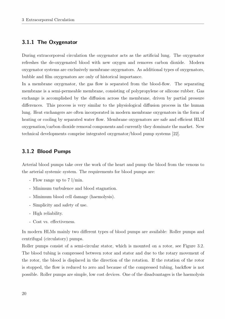
During extracorporeal circulation the oxygenator acts as the artificial lung. The oxygenator
refreshes the de-oxygenated blood with new oxygen and removes carbon dioxide. Modern
oxygenator systems are exclusively membrane oxygenators. As additional types of oxygenators,
bubble and film oxygenators are only of historical importance.
In a membrane oxygenator, the gas flow is separated from the blood-flow. The separating
membrane is a semi-permeable membrane, consisting of polypropylene or silicone rubber. Gas
exchange is accomplished by the diffusion across the membrane, driven by partial pressure
differences. This process is very similar to the physiological diffusion process in the human
lung. Heat exchangers are often incorporated in modern membrane oxygenators in the form of
heating or cooling by separated water flow. Membrane oxygenators are safe and efficient HLM
oxygenation/carbon dioxide removal components and currently they dominate the market. New
technical developments comprise integrated oxygenator/blood pump systems [22].
3.1.2 Blood Pumps
Arterial blood pumps take over the work of the heart and pump the blood from the venous to
the arterial systemic system. The requirements for blood pumps are:
- Flow range up to 7 l/min.
- Minimum turbulence and blood stagnation.
- Minimum blood cell damage (haemolysis).
- Simplicity and safety of use.
- High reliability.
- Cost vs. effectiveness.
In modern HLMs mainly two different types of blood pumps are available: Roller pumps and
centrifugal (circulatory) pumps.
Roller pumps consist of a semi-circular stator, which is mounted on a rotor, see Figure 3.2.
The blood tubing is compressed between rotor and stator and due to the rotary movement of
the rotor, the blood is displaced in the direction of the rotation. If the rotation of the rotor
is stopped, the flow is reduced to zero and because of the compressed tubing, backflow is not
possible. Roller pumps are simple, low cost devices. One of the disadvantages is the haemolysis
20

3.1 Principles and Components of the Extracorporeal Circuit
Adjustmentnut
Tubeguides
Tubingbushing
Roller
Backingplate
Rotationdirection
Outflow Inflow
Figure 3.2: Roller pump.
caused by the compression of the tubing. Furthermore a line restriction upstream will create
an excessive vacuum, leading to a degassing of the blood and a generation of a ’bubble train’
inside the tubing. Conversely, a line restriction downstream will lead to an immediate pressure
build-up, with possible dire consequences depending on the source of obstruction. A roller
pump displaces air and blood in the same way, which could lead to severe organ and tissue
damage when massive amounts of air bubbles are passed towards the patient.
In rotational blood pumps, a rotating impeller moves the blood in the desired direction by
centrifugal forces. In a centrifugal blood pump, the blood is drawn axially to the rotating axis
of the impeller and ejected tangentially. Due to the advanced design process (finite element
simulation methods), used for most modern centrifugal blood pumps, shear stress and turbulent
blood-flow are minimised. Amongst the most prominent advantages of these blood pumps are
the reduced haemolysis, the practical implementation, the long-life time, an only moderate
pressure rise on the occlusion of the arterial line and the small time constants (varying of course
on pump type). Disadvantages are the certainly higher costs (single-use product, pump head
or whole pump), a possible backflow at impeller cessation and the lack of a possible pulsatile
perfusion. Figure 3.3 shows the DeltaStream blood pump as an example for a rotary blood
pump with diagonally streamed rotor. The black arrows in Figure 3.3 indicate the direction of
blood-flow and the direction of the rotational speed of the pump impeller.
21

3 Extracorporeal Circulation
1
2
3
4
Figure 3.3: The DeltaStream blood pump as an example for a rotational blood pump. 1 is thedirection of blood inflow, 2 is the rotating impeller, 3 is the blood stream flowing around theimpeller, and 4 is the rotation direction of the impeller.
3.1.3 Tubing
Considering the fact that during ECC the blood is in contact with a large artificial surface
area (several meters of tubing), the defensive system of the human body may initiate multi-
ple biological reactions. Such defense reaction systems include for example the coagulation,
the fibrinolytic, the complement, the kallikrein and the kinin system [43, 112]. Systemic re-
sponse may be highly inflammatory and can affect heart, lungs, brain and other organs. Since
haemostatic mechanisms within the vascular endothelium are quite complex (and up to now
subject to research), a tubing coated with healthy vascular endothelium, would be the ultimate
biocompatible surface. State-of-the-art is the heparinisation of the blood and heparin-coated
biosurfaces. Clinical and research results of biosurfaces outline beneficial mitigating body de-
fensive system and coagulation response effects [132].
Although different tubing materials are available on the market, the tubing of choice is polyvinyl
chloride (PVC). Today heparin-coated biosurfaces are not only available for the tubing system
but for all other HLM components in contact with blood.
22

3.2 Pathophysiology of Extracorporeal Circulation
3.1.4 Other Components
Besides the main components, described above, various other components are used during
CPB. These include blood reservoirs, heat exchangers, arterial and venous cannulae, sensors,
measurement devices, device drivers, blood-gas analysers, infusion rate controllers and surgical
instruments. If needed for system modelling and automatic control, the components will be
described in detail in Chapter 4.
3.2 Pathophysiology of Extracorporeal Circulation
Pathophysiology of ECC can have different meanings. Physiology refers to the organ function
and regulation under normal conditions. Pathophysiology on the one hand is the abnormal
organ function, the degradation and the inadequate reaction of body organs in association with
the HLM. These are of course invoked by the artificial environment directly influencing hep-
atic, neurologic, renal, haemodynamic and other functions, but primarily by the mechanical
and pharmacological situation, inherent to the machine. On the other hand pathophysiology
can be the dysfunction of the extracorporeal artificial organ caused by a mechanical system
failure or by the inadequate managing of an operator.
The application of the artificial organ heart-lung machine in conjunction with a number of
cardiosurgical and anaesthetical procedures means a major alteration to body and organ func-
tions. Beyond that, CPB is applied in common to patients with cardiovascular or even multiple
diseases, which means a coupling with the pre-CPB pathophysiological situation.
The pathophysiological factors with reference to ECC are generally divided into certain medical
areas, as shown in Figure 3.4. In contrast to that, physiology and pathophysiology of ECC was
divided in the following points with respect to the automatic control aspect of this work.
- The artificial environment, with the major pathophysiological alterations.
- Pathophysiological response to ECC of transport functions of blood and blood loss.
- Blood component dysfunction, foreign surface interaction, haemolysis influences, etc.
- Organ changes and dysfunctions.
- Changes to the vascular system.
23

3 Extracorporeal Circulation
With regard to the main question ’what changes are introduced by CPB circulation and what
changes may occur on a particular dysfunction of the HLM’, the rest of the subsection is organ-
ised. Physiological and pathophysiological changes that occur during CPB and influence the
automatic control system are highlighted, where other non-influential effects may be neglected.
Anti-coagulation
Hypo-thermia
Haemo-dilution
Chirurgicaltrauma
Anesthesia
Haemo-dynamics
Diseases(cardiovasc.)
ECC
Figure 3.4: Pathophysiological factors for extracorporeal circulation (ECC).
3.2.1 The Artificial Environment
The artificially generated environment affects the patient’s physiological system by means of
changed conditions, like haemodilution, hypothermia and haemodynamics.
Haemodilution is the increase in the fluid content of the blood resulting from priming the HLM
with a priming solution fluid. The extracorporeal circuit needs to be primed with either donor
blood, isotonic saline or colloid solutions before establishing the CPB. Priming the blood with
substances other than donor blood is done to overcome the affiliated problems. An increased
viscosity, haemolysis, a transfusion reaction and the transmission of infections are the potential
risks if donor blood is used during hypothermia. These problems are overcome at the expense
of a decreased haematocrit (up to 20-50 % of the original value) and the risk of postoperative
damage, such as the formation of oedemas. On the other hand, the use of crystalloid or colloid
priming fluids decreases the blood’s viscosity and therefore works against the increasing viscosity
effect of hypothermia.
24

3.2 Pathophysiology of Extracorporeal Circulation
Induced hypothermia is the cooling of the blood and the human body. Common CPB ap-
plications of hypothermia range from moderate hypothermia (34 C) to complete circulatory
arrest (at about 10 C). Hypothermia is used in cardiac surgery to damp the metabolic rate,
protecting the tissue and the organs. Advantages of hypothermia are the decrease in the flow
rate due to a rise in the total peripheral resistance (TPR), which results in a lower traumatisa-
tion of the blood and in case of failure of the HLM in more patient safety because of the cooled
and protected organs, see Table 3.1.
Table 3.1: Percentile O2-consumption and time of HLM shutdown until tissue damage occurs underhypothermia [68].
Temperature O2-consumption Time of HLM shutdown[C] [%] [min]
37 100 4-529 50 8-1022 25 16-2016 12 32-4010 6 64-80
A disadvantage of hypothermia is the rise in the viscosity of the blood shown in Figure 3.5,
which can be compensated by blood priming. The effects of a left drift of the O2-saturation
curve due to low temperature can also be seen as a disadvantage since there is a decrease of
O2-delivery to the tissue. This disadvantage can be overcome by the adaption of O2-partial
pressures to the temperature. The sludging effect of the erythrocytes at low temperatures,
which can block the capillaries, is also lowered by the priming of blood.
The haemodynamics during CPB depend on the perfusion strategy and can be the greatest
artificially induced change. The ideal qualities of a blood pump are that of a heart: minimum
haemolysis, pulsatile flow and adjustable stroke volume. However, despite the advanced design
techniques of modern blood pumps, the blood is still damaged by shear stress occurring in
turbulent flows in the pumps and the extracorporeal circuit. The elements between arterial
blood pump and aortic input cannula (oxygenator and arterial filter, see Figure 3.1) prevent
a physiological pressure curve in the aorta, even if a physiological pulsatile flow curve is gen-
erated by the blood pump. The reason for this change is the additional resistance of these
elements and the impedance that changes the dynamics. The long existing debate of pulsatile
vs. non-pulsatile and centrifugal vs. roller generated flow has produced conflicting results
25

3 Extracorporeal Circulation
8
7
6
5
4
3
blood viscosity [mPa s]
at = 213 mPaτ
haematocrit = 40%
temperature [°C]
20 25 30 35 37
Figure 3.5: Increase in the viscosity with decreasing temperature (hypothermia), at a constant shearstress of τ [62].
[21, 30, 31, 89, 124, 131, 140].
In pulsatile vs. non-pulsatile flow, a key issue is the systemic vasoconstriction in certain local ar-
eas after application of CPB with the possibility of potential organ damage. It has been reported
that an increase of peripheral resistance due to multifactorial reasons, such as catecholamine
release, activation of the renin/angiotensin system, vasopressin release and local tissue factor
release occurs [126, 127, 128]. Additionally, the carotid baroreceptors are suggested to be in-
volved in the vasoconstriction process during non-pulsatile perfusion [7]. Pulsatile perfusion
increases the microcirculation and the local tissue metabolism postoperatively. However, most
patients do not suffer from non-pulsatile perfusion because of the use of vasodilative agents.
In addition to the typical advantages and disadvantages resulting from technical constitution,
roller and centrifugal blood pumps differ mainly in the affinity to microembolisation and haemol-
ysis. It has been reported that spallation is common with roller but minimal with centrifugal
pumps [98] and haemolysis is significantly lower with centrifugal pumps [40].
For the haemodynamic values during onset, maintenance and weaning of CPB, see Section 3.4
below.
3.2.2 Pathophysiological Response
The important changes in haemodynamics and the vascular system will be studied in an extra
section in this chapter. Additional changes in blood volume, blood hormone levels (endocrine),
fluids and electrolytes appear during CPB and may lead to significant pathophysiological re-
sponses.
26

3.2 Pathophysiology of Extracorporeal Circulation
The abnormally high release of endocrine hormones can be attributed to the shock-like stress
conferred by ECC. Hormone levels rise on the application of ECC and continue at a high
level after weaning. Antidiuretic hormone (ADH), renin, cortisol and catecholamine levels are
known to rise with induced anaesthesia and surgery alone. ECC further accelerates the distri-
bution of prostaglandins and serotonin, as well as the levels of epinephrine and norepinephrine.
The increased level of these hormones can be traced back to the application of hypothermia,
haemodilution and low perfusion.
Body fluid and electrolyte disorder have been observed during CPB [101]. After the application
of ECC the levels of extracellular fluid and exchangeable sodium were found to be increased,
where the total body potassium was decreased. Hypokalemia is of most important significance
because of the potential of developing arrhythmias.
To guarantee a satisfactory venous blood return to the HLM, lost blood volume resulting from
interstitial fluid shift and renal excretion has to be replaced adequately.
3.2.3 Blood Component Dysfunction and Oxygen Transport
The priming of the blood, blood haemolysis, fibrin formation and clotting as well as immune
defense response affect the different blood components and therefore also the haemodynamics
and the oxygen transport.
Haemolysis is the excessive breakdown of red blood cells (erythrocytes) and occurs in the
HLM in areas with high shear stress rates in the blood, i.e. in regions of turbulent flows.
High shear stress rates also damage other blood cells, which is not so critical in terms of
immunological or haemodynamical response. If erythrocytes are damaged or destroyed, the
contained haemoglobin is distributed to the blood plasma, where it is bound to haptoglobin.
If the binding capacities of the haptoglobin are saturated, the haemoglobin circulates in the
blood and is excreted by renal tubulus cells. In modern HLM systems haemolysis, should not
be a problem and the development of a deficiency of erythrocytes (anemia) is seldom. For
the modelling and control of blood-gas transport the decreasing haemoglobin value has to be
considered.
Foreign surface contact of the blood leads to platelet (thrombocyte) activation and the
formation of fibrin. Even though in modern HLM systems heparin-based and biocompatible
surfaces, as well as the application of heparin as an anticoagulant are available, the effects
27

3 Extracorporeal Circulation
induced by the complex multiple biological reactions involving whole defensive systems, such as
the coagulation, complement, fibrinolytic, kallikrein and kinin systems can only be reduced. If
anti-coagulation techniques are not properly applied, these systems may lead to the activation
and consumption of thrombocytes, the formation of fibrin and clotting and other biological
reactions, which may also affect heart, brain and other organs, known as systemic inflammatory
response or post-perfusion syndrome.
The immune defense response bases on an irritation of the defensive system due to ECC.
Tissue damage to the endothelium and the organs can be the result of the defensive action,
which can be damped by hypothermia and vasoconstriction. Microbiological defense by the
leucocytes as a part of the defensive system can also lead to tissue destruction.
Oxygen transport capabilities of the blood and of the oxygenator are changed at the onset
and degrade during CPB. Oxygen transport influencing variables can be seen from the oxygen
binding curve (refer to Figure 2.3) and are haemoglobin and temperature. The haemoglobin
content of the blood is changed at the beginning of CPB and changes slowly during CPB
(due to haemolysis, etc.). Degradation of oxygen transport capabilities can also depend on the
oxygenator. The diffusion capacities are known to degrade over the course of CPB because of
the blood clotting effect in the microporous membranes of the oxygenator [37]. This means
a change to the inherent system properties of the coupled oxygenator-blood system that is
important for automatic control and is modelled as uncertainty.
3.2.4 Pathophysiological Response of the Vascular System
The response of the vascular system to the application and maintenance of ECC is certainly
complex and constitutes a crossfire of different, superposed reactions and interconnections be-
tween those reactions and connected systems. Vasoactive substances and their effects on the
vascular system are covered in an extra section of this chapter (see below). Figure 3.6 shows
a principal haemodynamic course of a hypothermal CPB. After onset, the TPR drops and is
almost halved. The initial drop in TPR can be explained by the drop in viscosity because of
blood priming with non-sanguine fluids. Additional influences are applied hypothermia (paral-
ysis of vascular musculature), dilution of circulating catecholamines, the increased distribution
of histamine and the application of anaesthetic or vasoactive drugs (see below). There are other
factors that influence this process, but even the involvement of the above-named processes is not
28

3.2 Pathophysiology of Extracorporeal Circulation
clear up to now and subject to research [62]. The subsequent increase of TPR after onset can
be explained with an increased catecholamine release, a compartmental fluid shift, activation of
the renin/angiotensin system, vasopressin release and local tissue factor release. Furthermore,
arteriolar reactions on local metabolic activity, the acidity state, the amplitude of pressure and
flow and the formation of shunts have been suggested influential in TPR rise. The influence
of microcirculation on this process remains uncertain. The TPR of the vascular system as a
characteristic value can change up to and more than ±100 %, where most of the resistance
change is due to the arterioles and not due to the larger arterial blood vessels or the aorta. In
addition to the TPR, the compliance1 of the vascular system and the inertance2 of the fluid
have been reported to change during ECC [109]. Inertance changes are due to the blood prim-
ing and the changed physical characteristics (viscosity) during ECC. The vascular compliance
changes when vasoactive substances or anesthetics are applied (see below), however, not much
is known about other effects during ECC.
3.2.5 Organ Response
ECC involves the use of a prosthetic device and its main alteration to the physiological human
system is the contact of blood with a foreign artificial surface, which replaces the endothelial
surface and the reticulo-endothelial system. If properly used, that is if well-known perfusion,
pH and blood-gas management regimens are preserved, ECC keeps the functions of body or-
gans unchanged during the conduct of the extracorporeal procedure. However, decreased blood
volume (hypovolemia), caused by haemodilution and hypotension, hypothermia, non-pulsatile
perfusion, haemolysis and anesthetisation depending on pre-operative heart disease may result
in tissue damage, temporary or permanent neurological damage, single or multiple organ failure
and inflammatory response, depending on the length of CPB. Errors due to manually controlled
perfusion dynamics and blood-gases may contribute to this process. Prosthetic surface interac-
tion and blood exposure with the resulting blood component damage and complement and other
mediator activation can be identified as the major physiological alteration caused by ECC.
1The compliance in physiology is a measure for the distensibility of body structures. It is used for the charac-terisation and quantification of the elastic properties of the considered tissues.
2The inertance of a fluid is the effective mass for the modelling of the inertia when fluid acceleration is regarded.
29

3 Extracorporeal Circulation
TPR(mmHg/( ))lmin-1
Hct(viscosity)
buffer base(mmol l )-1
BP(mmHg)
CI(lmin m )
-1 -2
ECC flow(lmin m )
-1 -2
Onset Weaning
On bypass3
2
100
60
3020
0-5
3
2
1
time
Figure 3.6: Principal haemodynamic response during conventional cardiopulmonary bypass withhaemodilution, hypothermia and low flow, where CI is cardiac index, BP is blood pressure, TPRis total peripheral resistance and Hct is haematrocrit [62].
3.3 Anaesthesia for Cardiopulmonary Bypass
Anaesthetics and other drugs for CPB are administered in the commencement (pre-operative),
the running and termination (weaning) of CPB, but also post-operatively. Administration
is effected by inhalation and intra-venous injection. During ECC, the anaesthetist has to
guarantee a proper common anaesthesia by means of unconsciousness (hypnosis), painlessness
(analgesia), damping or disconnection of certain reflex activities and the reversible paralysis
of skeletal muscles (muscle relaxation). In addition, haemodynamics, blood-gases and other
ECC effects (hypothermia and haemodilution) have to be monitored to predict the distribution
and the effective circulation period of these substances (pharmacokinetics). Preliminarily to a
success of CPB is the knowledge of
- the haemodynamics in terms of cardiac disorders and the influence of the anaestheticprocedures
30
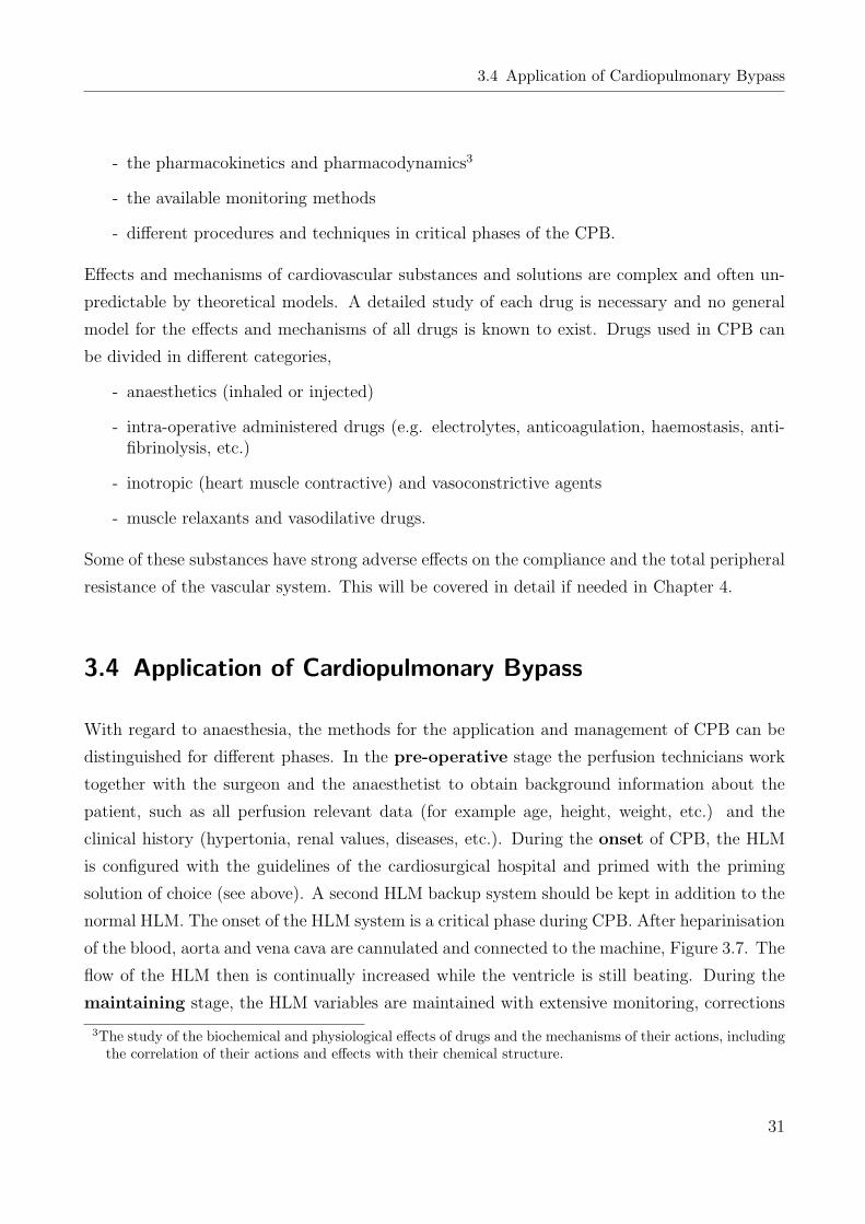
3.4 Application of Cardiopulmonary Bypass
- the pharmacokinetics and pharmacodynamics3
- the available monitoring methods
- different procedures and techniques in critical phases of the CPB.
Effects and mechanisms of cardiovascular substances and solutions are complex and often un-
predictable by theoretical models. A detailed study of each drug is necessary and no general
model for the effects and mechanisms of all drugs is known to exist. Drugs used in CPB can
be divided in different categories,
- anaesthetics (inhaled or injected)
- intra-operative administered drugs (e.g. electrolytes, anticoagulation, haemostasis, anti-fibrinolysis, etc.)
- inotropic (heart muscle contractive) and vasoconstrictive agents
- muscle relaxants and vasodilative drugs.
Some of these substances have strong adverse effects on the compliance and the total peripheral
resistance of the vascular system. This will be covered in detail if needed in Chapter 4.
3.4 Application of Cardiopulmonary Bypass
With regard to anaesthesia, the methods for the application and management of CPB can be
distinguished for different phases. In the pre-operative stage the perfusion technicians work
together with the surgeon and the anaesthetist to obtain background information about the
patient, such as all perfusion relevant data (for example age, height, weight, etc.) and the
clinical history (hypertonia, renal values, diseases, etc.). During the onset of CPB, the HLM
is configured with the guidelines of the cardiosurgical hospital and primed with the priming
solution of choice (see above). A second HLM backup system should be kept in addition to the
normal HLM. The onset of the HLM system is a critical phase during CPB. After heparinisation
of the blood, aorta and vena cava are cannulated and connected to the machine, Figure 3.7. The
flow of the HLM then is continually increased while the ventricle is still beating. During the
maintaining stage, the HLM variables are maintained with extensive monitoring, corrections
3The study of the biochemical and physiological effects of drugs and the mechanisms of their actions, includingthe correlation of their actions and effects with their chemical structure.
31

3 Extracorporeal Circulation
are made and the heart-surgery can take place. In the last stage, the weaning, the patient is
weaned from the machine.
3.4.1 Onset Stage
The onset begins with the configuration and installation of the HLM. Mainly two different HLM
structures are possible and used in modern HLM systems. In an open system, the venous return
and the sucker lines are returned to an open reservoir, from which the blood is pumped to the
arterial line. In a closed system, a closed soft bag and an open reservoir are connected to each
other (refer to Figure 3.1). Because of the venous soft bag the system is likely to collapse on
clearance and therefore closed for air embolism. After configuration and installation the HLM
is primed with donor blood or blood substitute substances. In addition to the heparinisation of
the patient’s blood, donor blood or priming substance in the HLM is heparinised. Hypothermia
is induced after application of ECC, which reduces coronary and bronchial backflow to the heart
Aorta
Truncuspulmonalis
(TP)
Right ventricle(RV)
Rightatrium(RA)
SVC
Venous outflow (VO)
Vena cava inferior (IVC)Vena cava superior (SVC)
IVC
RV
A
B
1
2
LV
D
C
Arterial inflow (AI)Clamp
Arterialcannula
Figure 3.7: Application of cardiopulmonary bypass, with venous cannulation to the left and arterialcannulation to the right, where the arrows for SVC and IVC are the corresponding venous flows.The points A)-D) on the right-hand side in the figure refer to the different cannulation techniques,for example for cardioplegia inflow 1) or left ventricle (LV) suction [129].
32
3.4 Application of Cardiopulmonary Bypass
and provides, with other advantages, better visibility conditions in the operating field.
3.4.2 Maintenance Stage
Extensive monitoring of different patient values is necessary to guarantee a successful and safe
CPB. Among the most important values are blood-flow, blood-gases (pO2 and pCO2), pressure
(arterial and venous), temperature, pH-value, coagulation/clotting status and urine excretion
rate. In addition to these values, the electroencephalography (EEG) can provide additional
information about anaesthetic conditions.
There is no international norm guideline for certain values, their maintenance and procedures.
However, recommendations that are based on clinical and physiological experiences exist (refer
to Table 2.2). Values such as oxygen partial pressure pO2 and arterial blood-flow qart have to
be adapted to artificial conditions depending on haemodilution and body surface (for example
pO2 ≈ 160 mmHg, pCO2 ≈ 40 mmHg, part ≈ 40-60 mmHg and qart ≈ 2.4 l/min/m2 body
surface are typical values). This adaption is achieved by the manual adjustment of control
variables, see Figure 1.1. The gas-flow to the oxygenator and the FiO2-value in the gas are for
example changed to achieve the right arterial blood-gas conditions. Additionally, the arterial
blood-flow may be changed to react appropriately to a change in the venous oxygen saturation
value.
For the blood-gas management during hypothermic CPB two methods exist. In the case of the
pH-stat method the measured values are corrected with translation tables to values at 37 C.
In contrast to the α-stat method, the pH-stat method needs the additional mixture and control
of CO2 gas in the oxygenator. The α-stat method uses (measures) and controls the values at
37 C and tolerates the shifting pH-values at lower temperatures. α-stat is the simpler and
more secure method because the blood-gases are given at 37 C and no correction is necessary.
Experimental measurements show [29], that α-stat keeps the cerebral auto regulation intact
(in contrast to pH-stat) and the global cerebral perfusion seems to be adopted to the patient’s
metabolic needs.
The above-named vital variables have to be continually observed and small to large adjustments
in the control values are needed to maintain these values under changing conditions. Even
under automatically controlled blood-gas and perfusion the perfusion technician is essential to
determine control setpoints and react to artificial disturbances (blood clotting, blood loss, etc.)
or unpredictable system failures (pump failure, blood-gas supply failure, etc.).
33
3 Extracorporeal Circulation
3.4.3 Weaning and Postoperative Stage
Weaning is the end of myocardial blood supply restriction (ischemia) up to the total discon-
nection of ECC. The oxygen consumption of the heart, represented by the heart muscle wall
tension, has to be kept at a minimum to avoid damage. A slow increase of heart ejection is
achieved by regulating the venous backflow to the heart and during that stage the blood and
the body are gradually rewarmed. Unphysiological pressures should be avoided until the HLM
is finally disconnected. The remaining blood in the HLM can be reconditioned.
After thorax occlusion, the patient is subject to intensive care and anaesthetic treatment, to
stabilise the haemodynamics and reduce the risk of post-operative damage and inflammatory
response.
During the weaning stage, the automatic control of the HLM can be further used by adapting
the control setpoint to required weaning changes.
34

4 Modelling of the System under Extracorporeal
Circulation
This chapter addresses system modelling under cardiopulmonary bypass (CPB) for the devel-
opment of control. Before introducing the models for haemodynamic and blood-gas processes,
a short section will address the control strategy. This control strategy section gives an overview
on control of CPB in literature, the suggested feedback variables, the control actuating princi-
ples and limitations, see Section 4.1 for the haemodynamic control strategy and Section 4.10
for the blood-gas control strategy.
The system is modelled in technical and physiological subsystems, which are interconnected
thereafter. The system modelling approach will consider haemodynamic modelling divided in
Sections 4.2-4.9 for each component first and is followed by the modelling of blood-gases in
the oxygenator, Section 4.11. In the oxygenator, the technical subsystem is coupled in an ex-
tracorporeal state with the physiological organ blood. Therefore, modelling of technical and
physiological parts will be done in the same section.
Each modelled subsystem follows a short simulation and validation in Chapter 5 ’Model vali-
dation’. Numerical constants are not included in this chapter and appear in Appendix B.
4.1 Haemodynamic Control Strategy
Different strategies on haemodynamic control of CPB exist in literature. The first applications
of automatic control date back to the 1960-70’s and were focused on the maintenance of an
appropriate pressure and flow in the venous return [130]. This was necessary since at that
time in most HLMs a venous withdrawal pump was used, which had to be monitored for safety
reasons (’venous chatter’). Several authors developed further control strategies, introducing PI
and rule-based control algorithms [17, 18, 35, 123]. Experimental implementation and in-vitro
tests produced good results. In these studies, flow in the central venous return was controlled
35
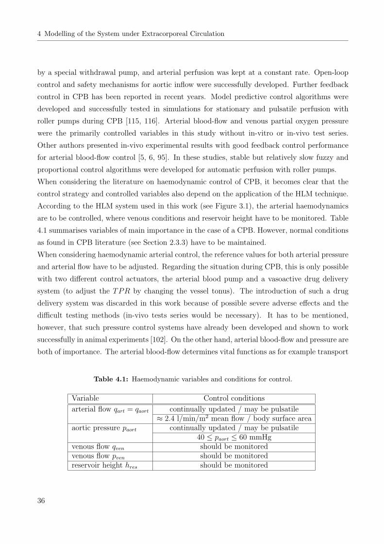
4 Modelling of the System under Extracorporeal Circulation
by a special withdrawal pump, and arterial perfusion was kept at a constant rate. Open-loop
control and safety mechanisms for aortic inflow were successfully developed. Further feedback
control in CPB has been reported in recent years. Model predictive control algorithms were
developed and successfully tested in simulations for stationary and pulsatile perfusion with
roller pumps during CPB [115, 116]. Arterial blood-flow and venous partial oxygen pressure
were the primarily controlled variables in this study without in-vitro or in-vivo test series.
Other authors presented in-vivo experimental results with good feedback control performance
for arterial blood-flow control [5, 6, 95]. In these studies, stable but relatively slow fuzzy and
proportional control algorithms were developed for automatic perfusion with roller pumps.
When considering the literature on haemodynamic control of CPB, it becomes clear that the
control strategy and controlled variables also depend on the application of the HLM technique.
According to the HLM system used in this work (see Figure 3.1), the arterial haemodynamics
are to be controlled, where venous conditions and reservoir height have to be monitored. Table
4.1 summarises variables of main importance in the case of a CPB. However, normal conditions
as found in CPB literature (see Section 2.3.3) have to be maintained.
When considering haemodynamic arterial control, the reference values for both arterial pressure
and arterial flow have to be adjusted. Regarding the situation during CPB, this is only possible
with two different control actuators, the arterial blood pump and a vasoactive drug delivery
system (to adjust the TPR by changing the vessel tonus). The introduction of such a drug
delivery system was discarded in this work because of possible severe adverse effects and the
difficult testing methods (in-vivo tests series would be necessary). It has to be mentioned,
however, that such pressure control systems have already been developed and shown to work
successfully in animal experiments [102]. On the other hand, arterial blood-flow and pressure are
both of importance. The arterial blood-flow determines vital functions as for example transport
Table 4.1: Haemodynamic variables and conditions for control.
Variable Control conditions
arterial flow qart = qaort continually updated / may be pulsatile≈ 2.4 l/min/m2 mean flow / body surface area
aortic pressure paort continually updated / may be pulsatile40 ≤ paort ≤ 60 mmHg
venous flow qven should be monitoredvenous flow pven should be monitoredreservoir height hres should be monitored
36
4.2 Centrifugal Blood Pump
of oxygen to and transport of carbon dioxide from the tissues, and related effects. The pressure
in the vascular system prevents the blood vessels from collapsing, therefore guaranteeing a
sufficient micro-circulation. Furthermore, the pressure determines together with the blood-flow
the delivered static and dynamic energy to the tissues. A direct pressure control, such as in
physiological perfusion achieved by the various regulation mechanisms of the human body, is
also desirable in CPB conditions. Bearing this in mind, a third control strategy was developed
in addition to an arterial blood-flow and an arterial pressure control strategy. For this, the
arterial blood-flow control was augmented with a pressure boundary control, with the arterial
blood pump as the only actuator [84]. The three control strategies are explained in detail in
Sections 6.1-6.2. For the haemodynamic modelling the haemodynamics of the HLM and the
vascular dynamics have to be considered, see below. Measured variables for feedback control
are the arterial line flow and pressure.
4.2 Centrifugal Blood Pump
Today, more and more rotary or centrifugal blood pumps are used in ECC. Since the advantages
of centrifugal blood pumps outweigh the disadvantages (Section 3.1.2), a centrifugal blood
pump was chosen as the haemodynamic control actuator. The Medos DeltaStream pump
is a centrifugal (rotary) blood pump with diagonally streamed rotor, see Figure 3.3. The
DeltaStream was chosen for this work because of the good (low) time constant, low haemolysis
and good controllability.
In order to achieve better control performance, an accurate model of the blood pump including
nonlinearities should be known. Only a few models developed for rotary blood pumps exist in
literature [24]. The nonlinear model developed in this work is based on experiments and is able
to predict outflow and pressure output over the whole range of static and dynamic conditions.
4.2.1 Brushless DC Motor
The rotary blood pump (DeltaStream, Medos AG, Germany) is driven by a brushless direct
current (BLDC) motor. The electrical and mechanical equations for the BLDC motor are
37

4 Modelling of the System under Extracorporeal Circulation
[71, 88]
(Jmot + Jload)dωmot
dt+ bmotωmot = Tmot − bloadωmot
Lmotdimot
dt+ Rmotimot = uin − uemf ,
(4.1)
where J is an inertia, b is a damping, T is a torque, L is the inductance, R a resistance
and u a voltage. The indices mot, load, in, emf refer to the motor, motor-load, input and
electromagnetic feedback, respectively. The electro-mechanical interconnecting equations for
Eqs. 4.1 are
Tmot = Kmotimot
uemf =2
3Kemfωmot,
(4.2)
where Kmot is the motor torque constant and Kemf the electromagnetic feedback gain. The
factor 2/3 is because of the three line coiling control of the motor. Figure 4.1 shows the electro-
mechanical connection of the BLDC motor elements. Rearranging Eqs. (4.1) and (4.2) gives
the following state space (SS) model in its linear representation
[dimot
dtdωmot
dt
]=
−Rmot
Lmot− 2
3Kemf
Lmot
Kmot
Jmot+Jload− bmot+bload
Jmot+Jload
[imot
ωmot
]+
[1
Lmot
0
]uin
y = [0 1]
[imot
ωmot
].
(4.3)
Rmot
JloadJmotbmot
Lmot
DC motor
Uemf
Uin
noutM
Figure 4.1: Equivalent electro-mechanical network diagram for the BLDC motor.
38

4.2 Centrifugal Blood Pump
Eqs. (4.3) are a linear second order SS system. However, certain elements comprise nonlinear
characteristics, which are either modelled to the SS representation or neglected, see below.
4.2.2 Centrifugal Pump and Nonlinear Motor Characteristics
A general nonlinear aspect of BLDC-motor systems is the temperature dependency of the
viscous damping bmot. Due to the cooling effect of the blood along the motor device, great
temperature changes in the DeltaStream centrifugal blood pump system do not occur and this
effect can be disregarded. The nonlinear effects following in this section were observed during
experiments and modelled in order to cope with experiments, where the experimental set-up
and methods are covered in Chapter 5.
In hydrodynamical centrifugal pump systems, the pressure output is dependent on flow and
rotational speed [24, 78]. Steady state gain measurements show that the hydrostatic pressure
difference between pump pressure at outflow and inflow can be characterised by a 2nd-order
polynomial, additionally dependent on pressure at pump inlet
pout = f1(qB, ωmot, pin),
where pin is the pressure at pump inlet and assumed to be constant. Figure 4.2 shows the non-
linear static transfer function as a function of pump flow and rotary speed (data of the Medos
DeltaStream was used for this figure). The second nonlinearity observed during measurements
was the changing damping in the TF due to turbulent flow conditions in the impeller. This
effect was first modelled as a changing damping of the load bload but later on neglected, since
there is no significant impact on the model.
In addition to the hydrostatic pressure output, the motor current limit is modelled as a nonlin-
earity. Here, the generated motor torque is not proportional to motor current, but a nonlinear
saturation function.
Tmot = f2(imot)
39

4 Modelling of the System under Extracorporeal Circulation
1000 2000 3000 4000 5000 6000 7000 8000
rotary speed [R/min]
pump flow [l/min]
500
400
300
200
100
0
-100
-200
pressure [mmHg]
0 l/min
4 l/min
Figure 4.2: Nonlinear static pressure output.
These two nonlinear effects can be described by the following equations
pout = f1(qb, ωmot, pin) = b2ω2mot + b1ωmot − b0qb + pin
Tmot = f2(imot) =
−amot ∀ imot ≤ −amot
imot ∀ −amot < imot < amot
amot ∀ imot ≥ amot
.(4.4)
Eqs. (4.4) lead to the following nonlinear state space (SS) model, which is shown in block
diagram form in Figure 4.3 [110].
[dimot
dtdωmot
dt
]=
−
Rmot
Lmotf2(imot)−
23Kemf
Lmotωmot + 1
Lmotuin
Kmot
Jmotf2(imot)− bmot
Jmotωmot
pout = [f1(qb, ωmot, pin)]
(4.5)
Eq. (4.5) is now a two input one output state space system, with pin assumed to be constant.
Note that the blood-flow input qb depends on the hydrodynamic characteristics of the arterial
and venous line of the HLM circuit and the human vascular system. In the steady state case,
flow depends on the total peripheral resistance (TPR) extended by HLM flow resistance and in
the dynamic case on total hydraulic impedance of the system. Also note that nonlinear effects
40

4.2 Centrifugal Blood Pump
of air inclusion in the pump head (impeller) that highly degrade the flow in the blood pump
are neglected. However, in such a case the whole HLM system has to be stopped as a severe
system failure and air bubbles in the blood have to be removed.
4.2.3 External Rotary Speed Controller
Most centrifugal blood pumps come up with a device driver unit with a rotational speed con-
troller, which is also the case with the Medos DeltaStream system. For the modelling, the
external rotary speed controller has to be taken into the model, where it was implemented to
cope with experiments. For rotational motor speed control of the blood pump, the angular
velocity ωmot is fed back to form the error of angular motor velocities emot
emot = ωr − ωmot
with the control reference signal ωr. A standard proportional plus integral (PI)-controller with
anti-windup saturation was placed in the feedforward path
C(s) =uin(s)
emot(s)= Kp
s + Ki
s, (4.6)
where C(s) is the PI-controller transfer function, Kp is the proportional and Ki the integral
gain. The controller parameters were tuned for the analogue pump system case. In order to
get a fast control response, the system described by Eqs. (4.5) was linearised at minimum
system gain qb → 0 l/min and no current saturation. The PI-controller was tuned for that
case using the root locus procedure with the help of the ’Control System Toolbox’ (MATLAB)
[70, 94]. Tuning the controller at an operating point (OP) with very low system gain leads
([i ] ,[u q ] )
w ''
mot mot
in B 1
in = const.
( ,q , p )wmot
B
[u , q ]'in Bx x
pout
Figure 4.3: Blockdiagram for the nonlinear state space system.
41

4 Modelling of the System under Extracorporeal Circulation
to underdamped system responses at system OPs of higher gain. However, the controller was
tuned to fit to measurement data and stability was ascertained in simulation over the whole
operating range of the blood pump model. By using the backward Euler integration method
[97],1
s≈ Tsz
z − 1(4.7)
the system was discretised with a sampling time constant Ts. The resulting difference equation
for the PI-controller is
uin(k) = fs [uin(k − 1) + Kp([KiTs + 1]emot(k)− emot(k − 1))] (4.8)
with k, the time of discrete sampling step instances and fs the anti-windup function. Anti-
windup is realised by means of a discrete integrator with saturation. With the substitution
x = uin(k − 1) + Kp([KiTs + 1]emot(k)− emot(k − 1))
follows the anti-windup to
fs(x) =
aω, ∀ x ≤ aω
x, ∀ aω < x < bω
bω, ∀ x ≥ bω
, (4.9)
with the PI-controller integrator limits aω, bω. The nonlinear centrifugal pump model with the
closed-loop rotary speed control circuit was implemented in MATLAB/Simulink and connected
to other HLM components, see Figure 4.6. System input is the rotary speed setpoint and the
blood-flow through the pump; system output is rotary speed and pressure at pump outlet.
4.3 The Oxygenator, Cannula and Tubing System
The arterial line components, following the blood pump are oxygenator/heat exchanger, tubing
system, arterial filter and aortic cannula, see Figure 3.1. These components affect the haemody-
namics by means of static flow resistance and impedance and have to be taken into the model.
Model data for the different components were either collected from data sheets or obtained by
experiments (refer to Chapter 5).
42

4.4 Vascular System Modelling - A Historical Review
The haemodynamics of the oxygenator/heat exchanger were modelled as a constant resistance
using measurement data over a wide operating range of different flows, where it showed a linear
behaviour. Although an oxygenator compliance could be measured in experiments [80], it was
neglected because it is about 100 times smaller than the compliance of the vascular system [20].
The tubing system was modelled by its constant fluid resistance and inertance. The formulas of
the linearisation process for parabolic wave flow profile were used to determine the parameters
[108, 122].
The arterial filter was modelled as a constant resistance; the arterial filter compliance, which
was determined during experiments and was about 1000 times smaller than that of the vascular
system, was neglected [20, 80].
A quadratic dependency of pressure drop on flow can be observed in the aortic cannula. Hence,
the resistance of the aortic cannula RC was modelled linearly dependent on flow
RC = aC1qB + aC0, (4.10)
where aC0 is the static resistance and aC1 is a parameter corresponding to the linear depen-
dency on blood-flow. These values were fitted to measurements1 and agreed when compared to
literature [20], see Figure 5.4.
The different components were connected in series and implemented as subsystems in the MAT-
LAB/Simulink block diagram.
4.4 Vascular System Modelling - A Historical Review
Starting with the beginning of the 20th century, various developments and improvements of
cardiovascular system modelling were made. The human vascular system and haemodynamics
were described in a very simplistic model, which incorporated the most important dynamics and
was called the ’Windkessel’ model [34]. In the late 1950s, system modelling based on the lin-
earisation of the Navier-Stokes equations started in linear vascular system modelling [103, 139].
With the advance of technology, models on analogue computers, hybrid system, hydromechan-
ical simulators, and discretised versions were developed [12, 106, 107, 121, 122]. In contrast to
a few highly detailed vascular system models, numerous approaches of cardiovascular system
18 mm arterial cannula, bent tip, Stockert, Munich, Germany
43

4 Modelling of the System under Extracorporeal Circulation
models (including venous return, pulmonary circulation, various nonlinear effects and pulsatile
heart) exist in literature. Almost all of the developed models are based on compartmental
analysis2, which has grown much in the last decades and has applications in different branches
of biomedical engineering [57]. The main aims of vascular system modelling were to develop a
strong theoretical background in either natural or pathological conditions, considering vascular
impedance, wave propagation and reflection, blood and injected substance volume distribution,
haemodynamic control, heart and vascular coupling and the observation of distinct system state
variables. Models were successfully developed, for example, for teaching purposes, control of
heart assist devices, total artificial hearts, or systemic properties in the state of extracorporeal
circulation [9, 10, 11, 23, 25, 38, 58, 64, 65, 75, 99, 106, 107, 111, 117, 118, 142]. Further
developments, addressing signal, pulsatility and nonlinear analysis have been made in the past
few years [92, 86, 114, 115, 119, 135, 137].
During ECC, vascular system parameters are subject to changes according to the artificially gen-
erated environment. Models addressing the coupling of the HLM with the patient’s system and
the artificially generated environment have been developed in recent years [15, 20, 92, 104, 115].
However, the level of details in those models varies widely, where some models are simplistic
but sufficient and others are detailed and nonlinear models of higher order. Only a few authors
validated their models with in-vivo measurements and almost none of those exist for the CPB
case. During CPB, additional complexities and changes arise, for example different effects on
vascular tonus have to be considered (refer to Chapter 3), for which no direct experiments or
experimental methods exist. Due to the application of CPB and the affiliated effects, vascular
resistance, compliance and inertance are changed. However, up to the present no model de-
scribing CPB or anaesthetic effects on the human vascular system in detail is available. The
complex mechanisms of various vasoactive substances are mostly modelled directly in single
model approaches [54] and are based on transport processes, volume distribution and recir-
culation of the drug. In this study, a compartmental volume distribution model [107], which
is coupled to the fluid-flow describing compartments is used. The system parameters of the
vascular fluid-flow compartments will be changed according to the vasoactive substance (see
below). The different effects on vascular tonus at the beginning of ECC can be described by
changing the vascular parameters and can be regarded as vascular system uncertainties.
In contrast to other cardiovascular modelling and simulation studies, the model in this study
2Compartmental analysis is the segmentation of a complex process into a finite number of subsystems, calledcompartments, which interact to each other by well-defined variables and are described by a set of mathe-matical equations.
44

4.5 The Vascular System
is developed and optimised for automatic control. Two approaches for vascular modelling are
chosen: A model of higher order and accuracy is used to describe the frequency-dependent
effects and will be compared to a low order approach. The model of choice is then extended
with certain nonlinearities and furthermore time-variant parameters dependent on vasoactive
substances are being studied. Frequency-dependent properties are modelled to a certain degree
only, since high frequency properties vary strongly and can be handled with robust control.
Even though implemented with modern computer technology, a high order system incorporat-
ing nonlinearities may lead to computational problems if used during real-time simulation and
control. It is suggested that the nonlinear vascular system can be described with a lumped
low order linear system containing the most important low frequency information [28] with
upcoming goals of adding certain nonlinearities and time-varying parameters.
In the next section, the Navier-Stokes equations are linearised with the finite difference method
and simplified to get the difference-differential equations for compartmental modelling [57].
4.5 The Vascular System
4.5.1 Fluid Flow in Elastic Tubes
For homogeneous, incompressible fluid flow through elastic tubes, the Navier-Stokes equation
(NSE) in the general form is [13, 36, 39]
∂v
∂t+ (v · ∇)v = −1
ρ∇ p +
η
ρ∆v + ff , (4.11)
where v is the velocity of flow, ρ is the fluid density, p is the pressure, η is the dynamic
viscosity and ff is the body force (units [N/m3]) applied to a volume element. ∇, ∆ are the
Nabla and the Laplace operator, respectively. For homogeneous, incompressible Newton fluids
holds ρ = const., η = const.. The continuity equation
∂ρ
∂t+ ρ ∇ v = 0 (4.12)
then becomes
∇ v = 0.
45

4 Modelling of the System under Extracorporeal Circulation
If it is assumed that no external force is applied to the blood vessels
ff = 0.
The simplified, still nonlinear, NSE is then
∂v
∂t+ (v · ∇)v = −1
ρ∇ p + ν∆v, (4.13)
with the kinematic viscosity
ν =η
ρ.
4.5.2 Simplified Electrical Analogue
To neglect the nonlinear terms of (4.11) and (4.12), which are the coupled wave velocities and
accelerations, it is assumed (and also shown, [103]) that the maximum and average velocities in
axial direction are small compared to the wave velocity and that the average radial velocity can
be neglected compared to the axial velocity. Linearising these negligible nonlinear terms, leads
to two joint second order partial differential equations [96, 108]. For the further transforming
of the equations to cylindrical coordinates, a parabolic flow profile and homogeneity, elasticity,
isotropy and the validity of Hook’s law for the vessel wall are assumed. Further neglecting the
second order partial derivatives and assuming an incompressible vessel wall results in two first
order partial differential equations,
− ∂p
∂xv
= L∂q
∂t+ R q
− ∂q
∂xv
= C∂p
∂t,
(4.14)
where p and q describe the pressure and flow along the coordinate xv, which is the axis in
flow direction. Note that Eqs. (4.14) do not depend on the radial axis, which is because of
the assumed parabolic flow profile. By applying the finite difference method using a Taylor
approximation [103, 139], Eqs. (4.14) are further simplified. Two location-dependent linear
difference-differential equations of first order are the result, which describe the flow and pressure
46

4.5 The Vascular System
in a tube compartment of finite length xv,
p(t|xv)− p(t|(xv + ∆xv)) = L ∆xvdq(t|xv)
dt+ R ∆xv q(t|xv)
q(t|xv)− q(t|(xv + ∆xv)) = C ∆xvdp(t|(xv + ∆xv))
dt.
(4.15)
Note that the p(t|xv) and q(t|xv) are time-dependent functions at location xv. In Eqs. (4.15),
L is the fluid inertance, C is the vascular compliance and R is the vascular resistance.
Finally the equations for the nth vascular compartment follow from Eq. (4.15) with the intro-
duction of subscript indices, substituting the length descriptions in brackets
pn − pn+1 = Lndqn
dt+ Rn qn
qn − qn+1 = Cndpn+1
dt,
(4.16)
where ∆xv is the the length of the discretised compartment. Variables p and q are time-
dependent. With ∆xvn , the parameters for compartment n are calculated
Ln =9ρ∆xvn
4πr2n
Cn =3πr3
n∆xvn
2Endn
Rn =81ν∆xvn
8πr4n
,
(4.17)
where En is Young’s modulus. Figure 4.4 shows the electric analogue for a vascular element,
where the pressure p = u and the flow q = i are according to a voltage and a current respec-
tively. Eqs. (4.17) are obtained in the linearisation procedure as given in [108]. Note that
np 1+np
nq 1+nq
nC
nR nL
Figure 4.4: Electric analogue for a single vascular element.
47

4 Modelling of the System under Extracorporeal Circulation
the parameters for the computation of the elements depend on the patient’s physiological and
pathophysiological vascular conditions and can vary strongly.
4.5.3 Vascular Model Structure
Eqs. (4.16) were Laplace transformed for one compartment.
Qn(s) =1
sLn + Rn
(Pn(s)− Pn+1(s))
Pn+1(s) =1
sCn
(Qn(s)−Qn+1(s)),(4.18)
where s is the Laplace operator. Eqs. (4.18) were implemented in a MATLAB/Simulink block
diagram as a transfer function. Figure 4.5 shows the Simulink block diagram, where pn and qn
Transfer function
1s
1
1
2
2
pn
pn+1
qn
qn+1
Gain Integrator
+_
+
1L s + Rn n
_Cn
-1
Figure 4.5: MATLAB/Simulink implementation for a basic compartment.
are the pressure and flow at the compartment’s input, pn+1 and qn+1 are the pressure and flow
at the compartment’s output.
4.6 Vasoactive Drug Extension
During ECC, the vascular system is subject to different vasoactive drug infusions. Vasoac-
tive drugs are specifically designed vasoactive agents, for either hypotensive or hypertensive
treatment. In most cases narcotic drugs also show an adverse vasoactive effect on the vascular
system, which is mostly of a dilative nature.
48

4.7 Volume Distribution Model
To describe the vasoactive influence on the vascular system dependent on time, a volume dis-
tribution model is incorporated in the vascular model. Distribution of the drug is modelled by
perfect mixing chambers, coupled to each vascular element. The time-varying nonlinear influ-
ence of the vasoactive drug agent on the vascular resistance and compliance is not precisely
known up to the present. There exists, however, a huge body of scientific and clinic applica-
tion studies of different vasoactive and narcotic drug application and central arterial pressure
control, for example [33, 42, 45, 54, 61, 67, 69, 141].
For the modelling of the drug influence, static TPR and compliance data from in-vivo mea-
surements, where the narcotic and vasoactive drug was applied, can be used. These results are
obtained from clinical studies and are used here to map the concentration of a certain vascular
compartment in a percentage change of the elements of that compartment.
4.7 Volume Distribution Model
In a vascular segment, the blood volume consists of unstressed and elastically stored volume.
The blood volume describing equation is [107]
VnT = VnU + pnCn, (4.19)
where the total volume VnT of compartment n is the sum of unstressed volume VnU plus the
elastically stored volume pnCn. Depending on the pressure in a vascular compartment, the
vessel distends and more volume is stored. The compliance that determines this stored volume
is assumed to be linear in its operating range. The concentration in each compartment is the
ratio of vasoactive substance volume V ∗n to total blood volume
c∗n =V ∗
n
VnT
, (4.20)
where the substance concentration is c∗n. With the substance concentration in each compart-
ment, the substance flow q∗n depends on the direction of blood-flow in that compartment [107]
q∗n =
c∗n−1qn ∀ qn ≥ 0
c∗nqn ∀ qn < 0. (4.21)
49
4 Modelling of the System under Extracorporeal Circulation
Finally the actual compartment substance volume is determined by the integral of the difference
of substance volume inflow and outflow
V ∗n =
t∫
0
(q∗n − q∗n−1)dt + V ∗n (0). (4.22)
A time constant k∗s,Drug, corresponding to the substance half-life time (HLT), has to be intro-
duced and Eq. (4.22) becomes
V ∗n =
t∫
0
(q∗n − q∗n−1 − k∗s,DrugV∗n )dt + V ∗
n (0). (4.23)
Eqs. (4.19), (4.20), (4.21) and (4.23) were implemented in parallel to the compartments of
the model and according to substance volume concentration of for example anesthetic or va-
soactive drugs the system parameters were changed. The parameters of the model therefore
change in dependence of drug application. Two functions, fR and fC map the vasoactive drug
volume in the different compartments to parameter changes of resistance Rn and compliance
Cn and are linear mappings fitted to practically measured data. That is K∗R,Drug = Rn/V ∗
n and
K∗C,Drug = Cn/V
∗n are constant gains, which cause percentage changes to the vascular para-
meters. Substance outflow at the venous return is fed back to the arterial inflow with a special
HLM compartment, describing the substance flow dynamics in the ECC circuit (tubing, venous
bag, etc., modelled with Eqs. (4.19), (4.20), (4.21) and (4.23)). Another variable parameter
is the HLT of the vasoactive substance. The integral time constant k∗s,Drug was obtained by
calculating the time constant of a first order differential equation for the HLT of the drug.
In the case of an injection of vasoactive drugs to the HLM, the substance distributes dynami-
cally over the vascular system, changing vascular resistance and compliance. Nonlinear effects
(e.g. saturation), as well as varying influence of the vasoactive substance to certain vascular
regions (e.g. venous or arterial system) are disregarded, since typical ranges for the injection are
kept during simulations. Note that the vascular system (Eq. 4.16) extended with vasoactive
substance distribution is thereafter nonlinear and its parameters are time-varying. In addi-
tion to that, uncertainty has to be assumed for the vascular parameters of different patients,
including different pathophysiological changes.
50

4.8 Model Interconnection and Augmentation
4.8 Model Interconnection and Augmentation
The model of the vascular system and the vasoactive substance distribution equations are
interconnected and augmented with the subsystems centrifugal blood pump (CBP), oxygenator
and arterial catheter.
The overall system can be described as a nonlinear time-variant multiple input, single output
system, with system uncertainties, including disturbances
x = f(x,u) + ∆f(x,u, t)
y = cx,(4.24)
where the state vector x consists of system’s flow, pressure, vasoactive drug volumes, pump
motor current, pump motor speed and controller output. Input vector u is the CBP input volt-
age for rotary speed reference and vasoactive drug or narcotic drug volume flow u = [ωmot V ∗in].
Output vector c is a linear mapping of the system state aortic inflow qaort or the system state
aortic pressure paort, depending on control usage of the model. System dimensions are u ∈ R2
(if only one vasoactive substance at a time is modeled) and y ∈ R. Note that the state dimen-
sion depends on the vascular compartment model, but is x ∈ R18 with the six compartment
model, see Chapter 5. f(·) and ∆f(·) are smooth nonlinear functions (i.e. f(·), ∆f(·) ∈ C∞).
∆f(·) contains the system uncertainties and functions for time-variant parameters.
Figure 4.6 shows the block diagram of the interconnected model for aortic blood-flow control
(with aortic flow as the output in this case). Blocks in double brackets represent system dynam-
ics with nonlinearities. pout is the pressure at pump outlet, paort the pressure at aortic input and
V∗s (Vasoactive Substances) the input vector of different substance volume flows. The transfer
functions ωmot-Control/M + BP/NPO, O + K and VS correspond to the rotary pump circuit
(speed controlled), the oxygenator and catheter and the vascular system augmented with vol-
ume distributions, respectively. NPO is the static nonlinear pressure output relation, described
by Eq. (4.4).
4.9 Modelling of Regulation Mechanisms
The regulation mechanisms of the body addressed in Section 2.5 react in a different way on
the vascular system than in physiological conditions. Local, neural, nerval and humoral control
51

4 Modelling of the System under Extracorporeal Circulation
-
ω(z) E(z) ωmot -control
U (z)inH
S / H
M + BP O + K VSQ (s)Aort.P (s)out P (s)Aort.ωmot(s)
HLM Patient
Vasoactivesubstances
NPO
Figure 4.6: Block diagram of the modelled system for haemodynamic control with different compo-nents. ωmot-Control: rotational PI-controller, H: hold element, S / H: sample and hold element,M + BP: motor plus blood pump, NPO: Nonlinear pressure output, O + K: oxygenator pluscannula, VS: vascular system.
of haemodynamics are all subject to the artificial environment during a CPB. The traumatic
stress, as induced by the opening of the ribcage, haemodilution and foreign surface contact of
the blood invoke different reactions of the control systems on the vascular system.
The nervous system can be assumed to be sufficiently damped to invoke strong reactions, but
the loss of vasoconstrictor tonus means an decrease of TPR. One of the most important in-
fluences on the vascular system during ECC is the catecholamine release, which is suggested
to depend on humoral and in parts on nervous control mechanisms. Catecholamine release is
opposed to the initial drop of TPR on the onset of ECC, which can be explained with other
superimposed mechanisms. Local haemodynamic tissue control is assumed to have little effect
on the vascular resistance and compliance, since different concentrations (main influence pH-
value) are kept at a physiological level (refer to Chapter 2).
Little is known about the different regulation mechanisms during ECC. Experimental stud-
ies measure the concentrations of different factors (e.g. catecholamines like epinephrine) but
reactions and interactions of the above-named mechanisms are hardly identifiable or quantifi-
able. Since general haemodynamics, like pressure and flow in the aortic arch, can be observed
during ECC with ease, the vascular parameters were assumed to have an extra uncertainty de-
pending on the haemodynamic regulation mechanisms. Figure 3.6 shows the haemodynamics
during CPB. According to the changes in pressure at constant blood-flow, TPR changes can
be determined. Uncertainties in resistance were assumed in the model and considered in the
robust control approach. Note that up to the present almost nothing is known about compli-
ance changes during ECC. Compliance uncertainties are assumed to exist and are based mainly
on observations of vasoactive substances, muscle relaxants or narcotics. These were of course
modelled as parameter uncertainties in the robust control approach.
52

4.10 Blood-Gas Control Strategy
4.10 Blood-Gas Control Strategy
For automatic control of blood-gases during CPB, only few approaches exist in literature.
Besides the control algorithms, different control inputs and sensors were used, as there are
certain different possibilities for this.
The control of oxygen delivery to the tissues, for example, was controlled with the blood-flow,
employed by [76, 77]. The process value hereby was the venous oxygen partial pressure. In
addition to that, venous carbon dioxide partial pressure was controlled with the total gas flow
through the oxygenator. This control strategy was avoided in this work since the change in the
blood-flow can lead to collapsing vessels (if too low) or cause vascular damage (if too high).
The control of venous blood-gas partial pressures was also avoided, since high and intoxicating
partial arterial pressures may occur, depending on the control input signal. A control of venous
blood-gas partial pressure with the oxygen fraction as the control input was developed in a
simulation study by [115].
With the control of arterial gas partial pressures in the blood an appropriate O2-supply and
CO2-removal can be guaranteed at a sufficient arterial blood-flow. As the control input for
arterial oxygen partial pressure pO2,a the O2-fraction in the gas-flow through the oxygenator
is often used. In contrast to that, the arterial carbon dioxide partial pressure pCO2,a in the
blood can be controlled by either applying CO2-gas to the gas-flow through the oxygenator or
by the total gas-flow. The implementation of such a strategy for O2-control only, was reported
by [4]. This study included a linear-quadratic-gaussian self-tuning control system and showed
good performance in in-vitro experiments. It was an improvement on former control strategies,
which mainly relied on linear PI, PID or piecewise linear control. Instability problems in these
studies occurred with linear controllers not properly tuned, or when process dynamics changed
[74]. A control strategy, where pO2,a is controlled by the control input oxygen-fraction FiO2 and
pCO2,a is controlled by the control input total gas-flow qg, seems to be most appropriate [46].
This control strategy is often used in cardiovascular surgery. The drawback of this method is the
coupled control input of gas-flow qg to the oxygen process input (see below) and the nonlinear
process characteristic. Despite these limitations that should be overcome with an advanced
control method, this control strategy has several advantages, such as: The good acceptance
and practical usage (up to the present this strategy is used for manual control); the saving
of an additional CO2-gas supply; a fast and reliable method to obtain almost physiological
blood-gas supply. For the modelling section below the control input for the oxygen process is
53

4 Modelling of the System under Extracorporeal Circulation
the oxygen fraction FiO2. For the carbon dioxide process the control input is the total gas-flow
qg. With these values the appropriate gas-flow through the oxygenator is adjusted by the gas
blender (see below). The arterial gas pressures pO2,a and pCO2,a are fed back as the process
values. Finally, reference values taken from CPB literature apply also for blood-gas control,
refer to Section 2.3.3.
4.11 Membrane Oxygenator Modelling
Blood-gas exchange in the lungs and transport of gas in the blood are difficult mathematical
processes incorporating nonlinearities and process time-delays. Blood-gases are exchanged in
the lung/oxygenator and the gases are transported to the body tissues via the blood stream.
The concentration of blood-gases in the venous blood depends on the metabolic activity of
the human body tissues. The oxygenation/carbon dioxide removal process in a membrane
oxygenator is similar to that in the human lung. For the modelling of the blood-gases during
ECC, a model that describes the dynamics of O2- and CO2-exchange [48, 49, 50] was adapted
to a membrane oxygenator system [47] and used for the development of an automatic control
strategy. Most important differences to the physiological lung blood-gas exchange are the
changed diffusion capacity of the oxygenator and the state of ECC. Hypothermia leads to a
left shift of the O2-binding curve and hypothermia together with anaesthesia reduce oxygen
consumption and carbon dioxide production in the tissues.
The modelling method for blood-gas exchange is compartmental modelling and is based on
the volume accounting equations of the compartments gas, plasma and red blood cells. Figure
4.7 shows a mixing chamber, as a generic compartment, with diffusion along the oxygenator
membrane. The equation that describes the component i is [47, 57]
Vmcd[C]idt
= qb,in[C]i,in − qb,out[C]i,out + Di(pi,ext − pi) + Ri, (4.25)
with Vmc, the volume of the compartment/mixing chamber, d[C]i, the concentration of compo-
nent i, qb,in, qb,out, blood in- and outflow and [C]i,in, [C]i,out, concentrations of component i at
in- and outflow (inflow concentrations of components correspond to venous conditions in the
membrane oxygenator). Di is the diffusion capacity over the oxygenator membrane and finally
Ri is a disturbance of the component i, corresponding to a loss or a chemical reaction. For the
54

4.11 Membrane Oxygenator Modelling
pi,ext
Di
pi
[C]iVmc
qb,outqb,in
[C]i,in [C]i,out
Blood
Membrane
Gas
Figure 4.7: Exchange of gases by diffusion over a membrane between blood and gas compartment.
modelling below, equations similar to (4.25) will be ordered in gas, oxygen and carbon dioxide
(and related) equations and perfect mixing of components will be assumed, i.e. [C]i,out = [C]i.
4.11.1 Gas Mixing Strategy
Most often the ventilating gas used for the oxygenation process in a membrane oxygenator is
a mixture of pure oxygen (O2) and a carrier gas, which is either nitrogen (N2) or ambient air
(21 % O2, 79 % N2). By adjusting the fraction of the pure O2-volume flow in the gas mixer
the oxygen fraction of the total gas stream that flows through the oxygenator can be achieved.
Possible FiO2-values depend on the carrier gas that is used. Values of FiO2 = [0.21 1] for
ambient air or FiO2 = [0 1] for N2 can be achieved. Higher oxygen fractions in the gas mean
higher partial pressures in the oxygenator gas compartment and therefore a higher diffusion
gradient, which leads in turn to a higher O2-partial pressure in the arterial blood. The oxygen
fraction in the gas is determined by both, the flow of oxygen (qO2) and the flow of carrier gas
(qN2) to the oxygenator. At a given total mixed gas-flow to the oxygenator qg, the flow of pure
oxygen is qO2 = FiO2 · qg and the flow of inert gas is qN2 = qg − qO2 , if nitrogen is the inert gas.
The oxygen fraction therefore is
FiO2 =qO2
qO2 + qN2
, (4.26)
which can range from 0 to 1 (or 0 - 100 %). Using Eq. (4.26) the setpoint values of the gas flows
of qO2 and qN2 are calculated according to the given values of FiO2 and qg. The gas flows are
then adjusted automatically by the gas valves, with a control routine already implemented in
the gas valves. During this control process an error in the lower operating range occurs, which
is due to the gas flow valves. This control error in turn leads to a static gain error and has to
55

4 Modelling of the System under Extracorporeal Circulation
be regarded in model validation (see Section 5.6) and control (see Section 6.3).
4.11.2 The Gas Blender
The mixing of oxygen and carrier gases in the blender is modelled as a perfect mixing chamber
with incorporated dynamics [46]
[FiO2(s)
qg(s)
]=
[1
Tg,bs+1e−Td1(qg)s 0
0 1Tg,bs+1
][FiO2,in(s)
qg,in(s)
], (4.27)
where FiO2,in is the fractional oxygen input, qg,in is the gas-flow input command signal, Tg,b is
the gas blender time-constant, Td1(qg) is the gas flow dependent time-delay and s is the Laplace-
transform variable. The time-delay Td1(qg) is a transport delay and is due to the distance from
gas blender to oxygenator. It applies to the oxygen fraction in the gas. The time-delay depends
on the gas-flow and the tubing system
Td1(qg) =π4d2
t,oxylt,oxy
qg
, (4.28)
where dt,oxy is the diameter and lt,oxy is the length of the gas tube between gas blender and
oxygenator. With higher gas-flows, the oxygen fraction time-delay drops to small values.
4.11.3 Gas Compartment
Two components are distinguished in the gas compartment, which are oxygen (O2) and carbon
dioxide (CO2). The gas fraction - partial pressure dependency (Henry’s law) is
pO2,g = pbarFiO2
pCO2,g = pbarFiCO2,(4.29)
where pO2,g, pCO2,g are the gas partial pressures, pbar is the atmospheric pressure and FiO2, F iCO2
are the mixing fractions of the respective gases. With the assumption qg,in = qg,out = qq and
56

4.11 Membrane Oxygenator Modelling
(4.29) the gas compartment describing equations are
VgFiO2
dt= qg(FiO2,in − FiO2,out)−DO2,m(pO2,g − pO2,b)
VgFiCO2
dt= qg(FiCO2,in − FiCO2,out)−DCO2,m(pCO2,g − pCO2,pl).
(4.30)
Note that FiCO2,in in (4.30) is assumed to be zero with the used control strategy (i.e. no
carbon dioxide is in the mixed gas). In the gas compartment model perfect mixing conditions
(FiO2,in = FiO2 and FiCO2,in = FiCO2) and no flow differences (qg,in = qg,out = qg) are
assumed. Substituting Eq. (4.29) into (4.30) and rearranging results in
VgdpO2,g,out
dt= qg(pO2,g,in − pO2,g,out)−DO2,mpbar(pO2,g,out − pO2,b)
VgdpCO2,g,out
dt= qg(pCO2,g,in − pCO2,g,out)−DCO2,mpbar(pCO2,g,out − pCO2,pl).
(4.31)
4.11.4 Oxygen Compartment
Total oxygen concentration [O2]b in the blood is the sum of dissolved and haemoglobin bound
oxygen,
[O2]b = αO2pO2,b + capbS(pO2,virt), (4.32)
where pO2,b is the partial oxygen pressure in the blood. The dissolved oxygen is determined
by the O2-solubility αO2 . Oxygen bound to the haemoglobin depends on the one hand on the
binding capacity
capb = hct · [Hb]rbc, (4.33)
in which hct is the haematocrit and [Hb]rbc is the haemoglobin concentration in the red blood
cells. On the other hand, the haemoglobin bound oxygen depends on the oxygen saturation
curve S(pO2,virt). For the oxygen saturation curve a virtual oxygen partial pressure pO2,virt. is
used, as the curve itself depends on a number of other variables (refer to Chapter 2)
pO2,virt. = xx = pO2,b · 100.024(37−Tb)+0.4(pHvirt−7.4)+0.06 log 40
pCO2 . (4.34)
57
4 Modelling of the System under Extracorporeal Circulation
In Eq. (4.36), Tb is the blood temperature, and pHvirt is the virtual pH-value (see below). With
the substitution xx = pO2,virt, the oxygen saturation curve is
S(xx) =a1xx + a2x
2x + a3x
3x + x4
x
a4 + a5xx + a6x2x + a7x3
x + x4x
, (4.35)
where aj, j = 1, 2..7 are numerical constants fitted to experimentally observed effects [63].
Assuming perfect mixing conditions, the oxygen compartment is described by
Vb
(αO2 + capb
∂S(xx)
∂pO2,virt
∂pO2,virt
∂pO2,b
)dpO2,b
dt= qb ([O2]b,in − [O2]b)+DO2,m(pO2,g−pO2,b), (4.36)
where [O2]b is described by (4.32) and Vb is the oxygenator total blood volume.
4.11.5 Carbon Dioxide Compartment
Carbon dioxide in the blood is transported in dissolved, bicarbonate ion (HCO−3 ) and in car-
bamate (carb) form, refer to Chapter 2. Within the carbon dioxide compartment reactions in
the plasma and the red blood cells (erythrocytes) have to be considered and are separated for
ease. In the following equations the dehydration of bicarbonate
RHCO3,pl = −kuαCO2pCO2,pl +kv
k[H]pl[HCO3]pl
RHCO3,rbc = cat
(−kuαCO2pCO2,rbc +
kv
k[H]rbc[HCO3]rbc
) (4.37)
is taken into account, in which k, ku and kv are the carbonic acid dissociation equilibrium, the
carbon dioxide hydration reaction forward rate and the carbon dioxide hydration backward
rate constant, respectively. In Eq. (4.37) cat is the carbonic anhydrase catalysis factor and
corresponds to the catalysed reaction by the enzyme carboanhydrase, which only exists in the
red blood cells. [H] is the hydrogen ion concentration. With the definitions for the plasma and
the red blood cell (erythrocytes) volumes and flows
Vrbc = hctVb, Vpl = Vb(1− hct), qrbc = qbhct, qpl = qb(1− hct), (4.38)
58

4.11 Membrane Oxygenator Modelling
the equations for the carbon dioxide transfer are
Vpld[CO2]pl
dt= VplαCO2
dpCO2,pl
dt
= qpl ([CO2]pl,in − [CO2]pl) +
DCO2,m(pCO2,g − pCO2,pl) + DCO2,rbc(pCO2,rbc − pCO2,pl) + VplRHCO3,pl
(4.39)
for the plasma part and
Vrbcd[CO2]rbc
dt= VrbcαCO2
dpCO2,rbc
dt
= qrbc ([CO2]rbc,in − [CO2]rbc) +
DCO2,m(pCO2,pl − pCO2,rbc) + VrbcRHCO3,rbc − Vrbcd[carb]
dt
(4.40)
for the red blood cell part. Note that Eq. (4.39) is directly coupled to the gas compartment by
the diffusion term DCO2,m(pCO2,g − pCO2,pl). The red blood cell compartment (4.40) is then
coupled to the plasma compartment by the interconnection term DCO2,m(pCO2,pl − pCO2,rbc).
In Eq. (4.40) [carb] is the carbamate concentration, interconnected to the plasma compart-
ment. The bicarbonate transfer equations for blood plasma ([HCO3]pl) and red blood cells
([HCO3]rbc) are
Vpld[HCO3]pl
dt= qpl ([HCO3]pl,in − [HCO3]pl)−
DHCO3,rbc
([HCO3]pl − [HCO3]rbc
r
)− VplRHCO3,pl
(4.41)
and
Vrbcd[HCO3]rbc
dt= qrbc ([HCO3]rbc,in − [HCO3]rbc) +
DHCO3,rbc
([HCO3]pl − [HCO3]rbc
r
)− VrbcRHCO3,rbc.
(4.42)
In Eqs. (4.41) and (4.42) r is due to a diffusion of [HCO3] across the membrane of the red
blood cells and some complex biochemical effects [49]
r = (0.058pHvirt − 0.437) S(xx)− 0.529pHvirt + 4.6. (4.43)
59

4 Modelling of the System under Extracorporeal Circulation
These effects are responsible for the virtual pH-value
pHvirt = − log (r[H]rbc) (4.44)
used in Eq. (4.36). The diffusion capacities DCO2,rbcand DHCO3,rbc
are estimated based on
in-vitro measurements [49]
DCO2,rbc= 0.693
αCO2
τrbc
VrbcVpl
Vrbc + Vpl
, DHCO3,rbc= 0.693
αCO2
τHCO3
VrbcVpl
Vrbc + Vpl
. (4.45)
In Eq. (4.45) τrbc and τHCO3 are the HLT of RBC membrane diffusion and RBC membrane
chloride shift, respectively. Within the carbamate reaction the carbamate is directly bound
in the red blood cells to the haemoglobin by the carbamino reaction
Vrbcd[carb]
dt= qrbc ([carb]in − [carb]) +
ka[CO2]rbcVrbc([Hb]− [carb])
(kzoS(xx)
kzo + [H]rbc
+kzr(1− S(xx))
kzr + [H]rbc
)−
Vrbcka[carb][H]rbc
kc
,
(4.46)
where ka, kzo and kzr are CO2-Hb forward reaction-time constant, oxygenated Hb amino group
ionisation- and reduced Hb amino group ionisation-constant. The exchange of hydrogen
ions, described by concentrations takes place in plasma ([H]pl) and red blood cells ([H]rbc) and
is of importance for the other reactions. The hydrogen ion concentration in the plasma
Vpld[H]pl
dt= qpl ([H]pl,in − [H]pl)− Vpl
2.303
βrbc
[H]rbcRHCO3,pl (4.47)
is influenced by the bicarbonate dehydration RHCO3,pl in the plasma, where in the red blood
cells hydrogen ion concentration
Vrbcd[H]rbc
dt= qrbc ([H]rbc,in − [H]rbc)−
Vrbc2.303
βrbc
[H]rbc
(−RHCO3,rbc + 1.5
d[carb]
dt− 0.6cap
dS(xx)
dt
) (4.48)
is influenced additionally by the carbamate d[carb]dt
and the oxygenation of Hb capdS(xx)dt
. In Eqs.
(4.47) and (4.48) βpl and βrbc are the plasma and the red blood cells buffer capacities.
60

4.11 Membrane Oxygenator Modelling
4.11.6 The Blood-Gas Analyser
In contrast to former blood-gas analysis (BGA), where blood samples had to be taken to special
BGA machines, modern blood-gas analysers are able to observe the blood-gas values pO2 and
pCO2 continually, at a predefined sampling time of Ts,BGA = 6 s. The blood-gas analyser used
in this study (CDI 500, Terumo, Japan) was modelled with a first-order lag differential equation
in the Laplace-domain
[pO2(s)
pCO2(s)
]=
[1
TBGAs+10
0 1TBGAs+1
][pO2(s)
pCO2(s)
], (4.49)
with TBGA = 20 s, the blood-gas analyser time constant for the partial pressure oxygen and
carbon dioxide input. The outputs pO2 and pCO2 are subject to an error due to amplitude
quantisation, because of discretisation, with quantisation interval 1 mmHg. A time-delay Td2(qb)
dependent on blood-flow and corresponding to the blood transport from arterial and venous
lines of the oxygenator to the BGA
Td2(qb) =π4d2
t,BGAlt,BGA
at1(0.01qb + at0), (4.50)
was introduced with the tubing length lt,BGA and the tubing diameter dt,BGA, where at0 is a
time-delay offset to prevent very large times-delays at zero flows. at1 is the conversion factor
from l/min to m3/s. With the time-delay (4.50) Eq. (4.49) becomes
[pO2,out(s)
pCO2,out(s)
]=
[1
TBGAs+10
0 1TBGAs+1
] [pO2(s)
pCO2(s)
]e−Td2(qb)s. (4.51)
4.11.7 Model Implementation and Generalisation
Eqs. (4.27) - (4.51) were implemented as subsystems in MATLAB/Simulink as shown in Figure
4.8. To get rid of the algebraic loop in Eq. (4.44), a first order differential equation with a fast
time constant was introduced in (4.44) to
dpHvirt
dt= 10 (−pHvirt − log (r[H]rbc)) . (4.52)
61

4 Modelling of the System under Extracorporeal Circulation
OxygenatorD + NL
pO2GBD
GBD
GBTD
BGAD TD + Q
pO2
pCO2
FiO2,in
Gas blender Oxygenator Blood gas analyser
qb
qg,in pCO2^
^FiO2
qg
Figure 4.8: Block diagram of the oxygenator system with, GBT: Gas Blender Dynamics, GBDT:Gas Blender Dynamics Delay-Time, Oxygenator D + NL: Dynamics and Nonlinearities, BGAD:Blood-Gas Analysis Dynamics and TD + Q: Time-Delay + Quantisation (and discretisation).
The resulting system is a three input, two output system, with inputs composed of the oxygen
fraction FiO2, the gas flow qg and the blood-flow qb, outputs composed of oxygen partial
pressure pO2, carbon dioxide partial pressure pCO2.
The system of Eqs. (4.27) to (4.51) can be substituted to a state space (SS) model of the form
(without time-delay)
x = foxy(x) + ∆goxy(x,u)
y = coxyx,(4.53)
where foxy(x) ∈ R15 is the new extended vector field, ∆goxy(x,u) ∈ R15 is the nonlinear in-
put vector field, containing the excerpted input terms and coxy ∈ R2×15 is the linear output
mapping. In Eq. (4.53) the state vector is x ∈ R15 and the output is y ∈ R2. foxy(·) and
∆goxy(·) are smooth nonlinear functions (foxy(·), ∆goxy(·) ∈ C∞). The model of (4.53) is re-
arranged in Section 6.3 to a single input-single output state-linearisation model (6.22). The
state-linearisation model (see below) has FiO2 input and pO2 output only and is reduced to 13th
order by neglecting the relatively small gas-blender dynamics. In contrast to that, the inputs to
the full process model are qb, FiO2 and qg and the output vector is yT =[pO2 pCO2
](without
sampling). To describe the real BGA-device (CDI 500, Terumo, Japan), the full process model
(4.53) is sampled at Ts,BGA with an output quantisation of 1 mmHg. For a detailed description
of the substituted state space model see Section 6.3.
62

5 Simulation and Experimental Model Validation
Models developed in Chapter 4, were validated in a simulation/experimental stage. For mea-
surement and control, the dSpace real-time environment1 was used for haemodynamic control
validation. For the blood-gas plant a special control software with an xPC Target control com-
puter was used. xPC Target provides a high-performance, host-target prototyping environment
that enables a connection of Simulink and Stateflow models to physical systems and executes
them in real time on PC-compatible hardware2. The experimental setup for blood-gas exchange
model validation is described in detail in Appendix D.3. The experimental setup for the vali-
dation of the haemodynamic model uses parts of the haemodynamic control validation model
(Appendix D.1). Pressures were measured with special pressure transducers and amplifiers3 and
with the DeltaStream Driving console (see below). The flow was measured using an ultrasonic
flow meter4. During all measurements tubing5 of 3/8’ was used. Details on the experimental
validation of different parts of the haemodynamic model are given below if needed.
5.1 Centrifugal Blood Pump and Rotational Speed Control
5.1.1 Experimental Setup and Methods
The DeltaStream blood pump system is a rotational blood pump with axially streamed im-
peller, including a driving device with speed control and parameter visualization6 [3]. The
1DS 1104 R&D controller board and CP1104 connector panel, dSpace, Paderborn, Germany2xPC Target, Mathworks, Natick, U.S.A3ISOTEC pressure transducer, TAM-A amplifier, Hugo Sachs Elektronik, Harvard Apparatus GmbH, March-
Hugstetten, Germany4T110 flow meter, 9XL flow probe, Transonic Systems Inc., Ithaca, NY, USA5Tygon, Raumedic, Helmbrechts, Germany6DeltaStream, Rotary blood pump and driving console, Medos AG, Stolberg, Germany
63

5 Simulation and Experimental Model Validation
DeltaStream system uses a Maxon BLDC motor with the digital electronic control unit includ-
ing the BLDC power amplifier7, [2]. For model validation, the pressures at pump inlet and
pump outlet were measured, using two DeltaStream pressure sensors. Rotary speed is directly
given by the DEC 50/5 control unit (with internal motor hall sensors).
All signals were discretised with the dSPACE real-time environment, at a sampling time of
Ts,cbp = 5 ms. During the measurements, the pump was tested at different hydrostatic pres-
sures at pump inflow, but also at different arterial line flow resistances.
The model was initialised with parameters from Maxon motor data sheets [1], given in Ap-
pendix B. Inertia of the pump impeller was theoretically acquired by standard formulas for the
geometric shapes of a cylinder and a truncated cone, see Figure 3.3. Formulas for the cylinder
and the truncated cone are [16]
Jcylinder =mcylinderr
2
2
Jtcone =3
10
r52 − r5
1
r32 − r3
1
mtcone
(5.1)
with the masses
mcylinder = ρπr2h
mtcone =1
3ρπh(r2
2 + r2r1 + r21),
(5.2)
where ρ is the density of blood. The whole inertia is composed of motor inertia, pump impeller
inertia and the motor rotor inertia (Jmot = Jcylinder + Jtcone + Jrot), which is simply denoted as
Jmot for the total inertia. Parameters for the nonlinear functions (4.4) were acquired by post-
processing of measurement data and polynomial fitting. During the measurements, a time-delay
of about Tt,m ≈ 40 ms occurred at the rotary speed signal. This time-delay originates from the
rotary speed measurement (hall sensors) at the µ-controller for measurement samples and is
therefore not modelled for control. The model was initialised with these parameters.
5.1.2 Experimental Results
Experimental results of the measurements are divided in time and frequency domain analysis.
To validate the system, two transfer functions can be distinguished (see also Figure 4.6). The
7DEC 50/5, Maxon, Sachseln, Switzerland
64

5.1 Centrifugal Blood Pump and Rotational Speed Control
dynamic BLDC motor transfer function (TF) is given by
Gmot(s) =ωmot
uin
. (5.3)
The dynamic plus hydrostatic nonlinear output TF is
Gcbp(s) =pout
uin
. (5.4)
Eq. (5.3) is used to validate the dynamic results of the BLDC motor including rotary speed
control. Eq. (5.4) contains the hydrostatic and dynamic system properties, as the pressure,
generated by the pump, is the system output. Frequency domain analysis is done for extreme
values of flow. The frequency responses are obtained using cross and power spectral density
of the Welch method [14, 52]. The experiment was set up using inductile tubes, with water
as pump medium. To keep the pressure at the pump inlet constant, a water reservoir with a
capacity of VW was used and filled with 1.6 l of water. The experimental setup was similar to
Figure 5.3, without the component tested.
Measurement data was collected by generating a sinusoidal chirp signal as the blood pump
input voltage, which leads to a rotary speed output around ωmot = 4000 Rmin
± 500 Rmin
. The
experiment was repeated for the open and closed (clamped) tube. In data post-processing,
the average mean of both input and output times series signals were removed and frequency
response data compared to the model results. Coherence function values did not drop below a
value of 0.9 in the frequency range up to 20 Hz.
Figure 5.1 shows the frequency response plot for TF (5.3). In the case of static gain and
resonance frequency the model matches the experimental data very well, in terms of system
damping the frequency response of the experimental data shows a more underdamped result.
The large phase drop at higher frequencies results from the measurement time-delay in the
motor revolution processing devices (see above). Figure 5.2 shows the time domain results for
static and dynamic system behavior and zero flow q = 0 l/min condition. The upper figures
correspond to the transfer function of Eq. (5.3), the lower figures to Eq. (5.4). By exchanging
the system parameters, the model can be easily adapted to different rotary pumps. However,
the lower damping of the resonance frequency at q = 0 l/min has to be taken into account for
control design, but because of much more bandwidth, TF (5.4) for maximum flow will be used.
65

5 Simulation and Experimental Model Validation
gain [dB]90
80
70
60
50
40
30
100 101
frequency [Hz]
phase [deg]
100
0
-100
-200
-300
-400
-500
-600
q = 0 (experiment)q = max (experiment)q = 0 (model)q = max (model)
q = 0 (experiment)q = max (experiment)q = 0 (model)q = max (model)
Figure 5.1: Experimental and simulation frequency responses for the TF of Eq. (5.3).
5.2 Oxygenator, Arterial Filter and Cannula
In contrast to the aortic cannula, which was modelled as a resistance linear-dependent on flow,
the oxygenator and the arterial filter were modelled as constant resistances (see Section 4.3).
Oxygenator, arterial filter and cannula were analysed in static and dynamic measurements.
Dynamic measurements showed a negligible dependency on frequency, and therefore dynamics
were neglected in the modelling (Chapter 4). Figure 5.3 shows the measurement setup for
the oxygenator and catheter experiments. A polynomial fitting, with a linear dependency
of the arterial cannula resistance on flow was obtained with measurement values, see Figure
5.4. Although a compliance of the arterial filter and of the oxygenator were measured in the
experiments, see Figure 5.3, the compliance was neglected, as they are small compared to the
compliance of the vascular system.
66

5.3 Vascular System Validation
5 10 15 20 25 30 353000
4000
5000
6000
7000
8000
simulation outputmeasurement output
rotary speed [R/min]
time [s]15 15.2 15.4 15.6 15.8 16
5000
5500
6000
6500rotary speed [R/min]
time [s]
simulation outputmeasurement output
5 10 15 20 25 30 350
50
100
150
200
250
300
350
400
450
500
P [mmHg]out
time [s]
simulation outputmeasurement output
15 15.2 15.4 15.6 15.8 16150
200
250
300
time [s]
simulation outputmeasurement output
P [mmHg]out
Figure 5.2: Static and dynamic simulation and experimental results for q = 0 lmin−1 of Eq. (5.3)and (5.4).
5.3 Vascular System Validation
The equations (4.18) given by the linearisation process are used for the vascular system mod-
elling. Two different kinds of models were developed and implemented in Simulink:
1. Following Avolio’s [12] detailed and complex 128-compartment approach, the arterial tree
is split into different elements, which are interconnected to each other. Parallel intercon-
nection is solved using the superposition principle, that means adding the back-propagated
flow of those elements in parallel. Parameters of the model (inertance, compliance and
resistance) were calculated with the vascular data of Avolio [12], Noordergraf [96] and
67

5 Simulation and Experimental Model Validation
Reservoir
CBP UFs
Ps1
Ps
Ps2 Ps3
Component
Ps4
Tubing
Tubing
Oxygenator
Syringec
(a) (b)
Figure 5.3: Experimental setup for the measurement of a component’s hydrodynamic parameters(a) and compliance of a component (oxygenator) (b), with Ps: the pressure sensors, UFs: theultrasonic flow sensor, CBP: the centrifugal blood pump, and c: T-connector.
Westerhof [138]. The model includes systemic arterial circulation only and is of 256th
order.
2. The second approach uses the parameters of Reul’s lumped model of human systemic cir-
culation [106]. The model consists of five different compartments in serial interconnection,
which represent aorta, arterial and venous circulation. The lumped parameters were orig-
inally estimated by Reul in an iterative process, to suit data from in-vivo measurements.
The model is of 9th order and includes venous circulation and venous return.
5.3.1 Experimental Setup and Methods
Both of the models were initialised from parameter files, containing compartment data for pa-
rameter calculation in the case of the 128-compartment model and experimentally estimated
parameters in the case of the five-compartment lumped model.
The 128-compartment model was furthermore reduced from 256th to 70th order. For this pur-
pose, Laplace-domain pole-zero pairs under a certain tolerance threshold were eliminated in a
first step. In a second step, the balanced model realisation with diagonal controllability- and
observability-Gram-matrices was calculated and further states with a small numerical values
in the Gram matrix (representative for combined controllability and observability) were elimi-
nated [51, 78, 145].
The three different systems are then compared in the frequency domain and finally simulated
with physiological pulsatile pressure curves. For the frequency response of the vascular system,
68

5.3 Vascular System Validation
0 1 2 3 4 5 60
5
10
15
20
25
30
35
pressure [mmHg]
flow [l/min]
polynomial fittingexperiment
Figure 5.4: Polynomial nonlinear pressure fitting for the arterial cannula, 8 mm bent tip, Stockert,Munich, Germany.
the system’s transfer function, corresponding to the system impedance is
Zvasc(s) = Gvasc(s) =Paort(s)
Qaort(s), (5.5)
where Paort(s) and Qaort(s) are the Laplace-transformed pressure and flow at the descending
aorta. Units of pressure and flow are [p] = mmHg and [q] = l/min. The unit of the magnitude
of impedance |Zvasc(jω)| is then [|Zvasc(jω)|] = mmHg/(l/min) and corresponds to a resistance.
Magnitude and phase are defined as
|Zvasc(jω)| = Magnitude,
arg(Zvasc(jω)) = Phase.(5.6)
5.3.2 Simulation Results
Figure 5.5 shows the results of frequency response validation of the models, varying in com-
plexity and order. In the frequency range of interest, f ≈ [0..15] Hz (but even up to 30 Hz),
where the most important cardiac output harmonics appear, all three models do not differ
much. The variations in magnitude and phase occurring in the higher order models depend
on the branching structure of the human arterial tree. However, main magnitude and phase
information at low frequencies is contained by the lower order model (disregarding any of the
69

5 Simulation and Experimental Model Validation
higher 256 order modelreduced 70 order modellow order model
magnitude [mmHg/(l/min)]30
25
20
15
10
5
0
-5
phase [deg.]
80
60
40
20
0
-20
-40
-60
0 2 4 6 8 10 12 14 16
frequency [Hz]
Figure 5.5: Impedance spectra of the simulated vascular models.
nonlinearities in all of those cases). The variations in the amplitude have to be considered for
control and are modelled later on as uncertainty.
Applying a certain cardiac output pressure curve as the vascular aortic input and using aortic
flow as the output, the three different models were compared in the time domain. The aortic
output pressure signal was generated with a pulsatile heart model [135]. Average mean aortic
input pressure is paort ≈ 100 mmHg and heart frequency is fht ≈ 70 BPM (beats per minute).
The resulting mean aortic inflow is qaort ≈ 4.4 l/min with both the complex 256th and the re-
duced 70th order model and ≈ 3.7 l/min with the low 9th order model. The difference between
the two models is due to different parameters of the vascular tree, resulting in a different TPR.
Inflow of the two vascular arterial models of higher and reduced order does not differ much, but
compared to the low order vascular model, depicted in Figure 5.6, the flow shape of the higher
order models shows stronger variations (depending on reflections of the human arterial tree).
Included in Figure 5.6 is also the mean venous flow, taken from the low-order vascular model.
Venous flow does not differ much, because of the larger time constants of that transfer function
(note that parameters for the models from which the frequency responses were calculated are
70

5.3 Vascular System Validation
0
0
0.5
0.5
1
1
1.5
1.5
2
2
2.5
2.5
3
3
3.5
3.5
4
4
4.5
4.5
5
5
60
70
80
90
100
110
120
130
-10
0
10
20
30
40
50
60complex order modelreduced order modellow order modelmean average venous flow
time [s]
Time [s]
aortic pressure [mmHg]
aortic flow [l/min]
Figure 5.6: Time series of the three different vascular models of the aortic pressure as input (upperpart) and corresponding aortic flow (lower part).
for the physiological parameter case. By changing the resistances and compliances, the models
were then adapted to the pathophysiological conditions that occur during ECC. This is shown
below).
5.3.3 Comparison of the Simulation Model and a Hydrodynamic Vascular
Simulator
Frequency responses of the linear 70th and 9th order systems were calculated and compared to a
hydrodynamic vascular system simulator (MOCK). This MOCK was developed and designed at
the Department for Biomedical Engineering, Ruhr-University-Bochum [91], refer to Appendix
D.1. In frequency response tests, the MOCK was validated against other higher-order models
and showed good agreement in a frequency range f = [0..15] Hz. At higher frequencies, dy-
namic effects of the measurement equipment (especially pressure sensors) appear and lead to
an amplitude damping and a phase drop. The magnitude and the phase of the three simulated
71
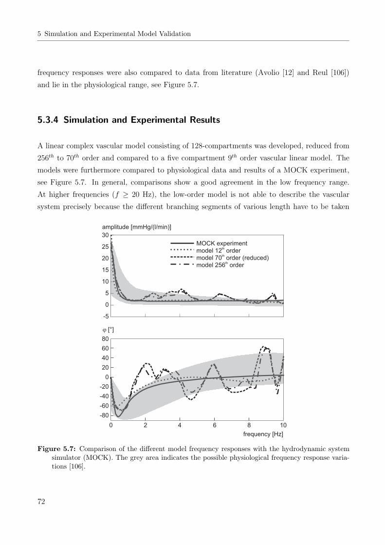
5 Simulation and Experimental Model Validation
frequency responses were also compared to data from literature (Avolio [12] and Reul [106])
and lie in the physiological range, see Figure 5.7.
5.3.4 Simulation and Experimental Results
A linear complex vascular model consisting of 128-compartments was developed, reduced from
256th to 70th order and compared to a five compartment 9th order vascular linear model. The
models were furthermore compared to physiological data and results of a MOCK experiment,
see Figure 5.7. In general, comparisons show a good agreement in the low frequency range.
At higher frequencies (f ≥ 20 Hz), the low-order model is not able to describe the vascular
system precisely because the different branching segments of various length have to be taken
30
25
20
15
10
5
0
-5
80
60
40
20
0
-20
-40
-60
-80
amplitude [mmHg/(l/min)]
frequency [Hz]
0 2 4 6 8 100 2 4 6 8 10
MOCK experimentmodel 12 ordermodel 70 order (reduced)model 256 order
th
th
th
j [°]
Figure 5.7: Comparison of the different model frequency responses with the hydrodynamic systemsimulator (MOCK). The grey area indicates the possible physiological frequency response varia-tions [106].
72

5.3 Vascular System Validation
into account (higher frequency modes). Higher-order complex n-compartment models can be
used for wave propagation, precise analysis of perfusion and pressure curves at certain vascular
segments or simulation of pathological vascular conditions. They are, however, unsuitable for
real-time applications, such as adaptive control and parameter- or state estimation. Adding
nonlinearities to these complex models would demand even further calculation cost and would
make the application of hardware in the loop or similar real-time strategies impossible, even
with today’s advanced computer technology. Since the modelling of the different branches relies
on the superposition principle, the extension of the model with nonlinearities in certain vascular
branches (such as renal perfusion) would lead to errors. As robust control is later on developed
to reject higher-order frequency uncertainties, the MOCK circuit can be used as an adequate
simulation device (note that resonance frequencies depending on turbulent flows also appear in
the MOCK). Critical parameter changes or differences affect mostly low-order frequencies and
can therefore be simulated by changes in the MOCK elements.
To develop and validate control algorithms for central arterial flow and pressure control, low-
order linear models with parameter initialisation depending on patient’s age, gender, weight,
height, hypothermia status and blood or priming fluid properties are sufficient to describe
the complex vascular system at a distinct operating point for a short time. Nonlinearities
depending on these parameters can be merged as parameter uncertainties to simplify simulation
and modelling. However, to implement automatic blood-flow or pressure control (BFC/BPC)
during all phases of CPB, more, and especially nonlinear and time-varying system knowledge is
needed. In the case of the human vascular system, flow- and pressure-dependent nonlinearities
can be disregarded [28]. Parameter uncertainties and nonlinear disturbances must still be
taken into account, for robust control synthesis. For BFC/BPC, parameter variations for the
above-named nonlinearities are considered as slowly time-varying effects. They are therefore
assumed to be persistent over a time and can be sufficiently modelled by parameter changes.
The distribution of vasoactive drugs in the vascular system, dependent on flow and pressure,
will be considered and has to be taken into the model (see below).
Based on the developed nonlinear model, including the HLM-components and the vascular
system, an analysis of nonlinearities with added uncertainties will be necessary to guarantee
robust stability and performance (see below).
73

5 Simulation and Experimental Model Validation
5.4 Vasoactive Substance Volume Extension
The vascular system of 9th order, consisting of equations (4.16), was coupled with vasoactive
substance distribution equations (4.19) - (4.23). Different vasoactive substances (anaesthetic
and vasoactive drugs) can be modelled in terms of different half-life times and changes of the
vascular elements (vascular resistance and compliance). Drugs that are used during a CPB can
be found in literature, stating the main influence on the vascular elements [32, 68, 129]. These
drugs can be divided into the following categories: Injection narcotic, inhalation narcotic, mus-
cle relaxant, cardiovascular (CV) and vasodilator drugs. Following these categories, the drugs
with certain impact on the vascular system were examined and modelled to the vascular com-
partment system. To give an example of the vascular effect on haemodynamics, two vasoactive
substances for simulation were chosen. The vascular resistance decreases with vasodilative sub-
stances and increases with vasoconstrictive substances. For the controlled aortic flow, a lower
TPR means a higher system gain in the TF (5.5) and therefore control destabilisation (in most
cases expressed with less gain and phase margin).
A few of the vasodilative substances lead to a rise in the compliance of the vascular system
(in total). A higher compliance mostly results in a shift of the resonance frequency (to lower
frequencies) and small changes in the system damping. Two vasoactive substances were chosen
as exemplarily for simulation for the following reasons.
1. Propofol, as an injection narcotic influences both TPR and aortic compliance strongly
with more than 100 % change as an adverse effect [69]. It is a hypnotic only and not
analgetic. Propofol is used mostly for initiation and maintenance of anaesthesia, together
with opiates. Amongst various benefits are that it is non-cumulative and allows rapid
initiation of anaesthesia and a smooth awakening on discontinuation of perfusion.
2. The other vasoactive substance for simulation is sodium nitroprusside (SNP), which shows
a strong effect on vascular resistance (effects on vascular compliance are also reported,
[105]). SNP acts as a pure vasoactive agent and is used in the treatment of hypertension.
It causes a relaxation of the peripheral vasculature muscles, which leads to strong blood
pressure reduction. The vasodilative effect is dosage-dependent. Special care must be
taken to avoid intoxication at dose rates > 1 µg/kg body weight.
The vascular model of Eq. (4.16), coupled with vasoactive substance distribution Eqs. (4.19) -
(4.23), is initialised with parameters corresponding to the vasoactive drugs (see Appendix B).
74

5.4 Vasoactive Substance Volume Extension
As shown in Figure 5.8 and 5.9, the input to the vascular model is a step in the vasoactive sub-
stance infusion rate, at constant blood perfusion. In Figure 5.8, the vascular system response
to a Propofol infusion is shown. Note that for simplicity reasons and in contrast to other mod-
elling approaches for vasoactive substances [54, 61], in this model the percentage changes in the
vascular parameters are linearly depending on vasoactive substance concentrations. Additional
nonlinear dynamics and gain (saturation), depending for example on recirculation are discarded
here. Depending on pressure and flow conditions at the time of injection, the vasoactive volume
distributes over the vascular system, causing a decrease in pressure and an increase in blood-
flow. The differences between Propofol and SNP injection can be seen in Figure 5.8 and 5.9.
These are the HLT and the percentage gain, that are due to the changed resistances and com-
pliances. Vasoactive substance infusion simulations like those shown in Figure 5.8 and 5.9 were
used to validate the robust stability of the haemodynamic controllers (see below). Controllers
developed in Section 6, were designed regarding vascular parameter changes (see Section 5.5 on
model linearisation below).
0.25
0.2
0.15
0.1
0.05
0
100
80
60
40
5
4
3
2
arterial linearterial system
0 100 200 300 400 500 600time [s]
propofol injection [mg/s]
p [mmHg]
q [l/min]b
Figure 5.8: Response to a propofol injection impulse with pressure and flow time series.
75

5 Simulation and Experimental Model Validation
0.02
0.015
0.01
0.005
0
100
80
60
40
5
4
3
20 100 200 300 400 500 600
time [s]
SNP injection [mg/min]
arterial linearterial system
p [mmHg]
q [l/min]b
Figure 5.9: Response to a sodium nitroprusside injection impulse with pressure and flow time series.
5.5 Model Linearisation
To analyse the influence of the different nonlinearities and uncertainties, the 18th order model of
Eq. (4.24) was linearised at a number of certain operating points. In addition, the parameters
of the vascular system were changed to cope with the observed effects on haemodynamics. The
model linearisation yields the linear system
x = A(t)x + B(t)u
y = cx,(5.7)
with the approximate Jacobians
A(t) =∂f(x,u)
∂x
∣∣∣∣x=xL,u=uL
+∂∆f(x,u, t)
∂x
∣∣∣∣x=xL,u=uL
B(t) =∂f(x,u)
∂u
∣∣∣∣x=xL,u=uL
+∂∆f(x,u, t)
∂u
∣∣∣∣x=xL,u=uL
,
(5.8)
76

5.5 Model Linearisation
where xL are the system’s state conditions for linearisation and uL are the input linearisation
conditions for the input vector. The influence of the vasoactive substances with time was ne-
glected (time dependency in the Jacobians), as the maximum change in the vascular parameters
at time tvasc was modelled as additional uncertainty. Eq. (5.7) therefore becomes
x = Ax + Bu
y = cx,(5.9)
with time parameter in Eq. (5.8): t = tvasc. Nonlinearities in Eq. (4.24) were analysed in
a loop linearisation procedure, where the states that influence the nonlinearities are changed
over a broad range. The vascular parameters were adapted to haemodynamics during ECC and
additional uncertainty was applied: TPR and compliance were changed up to 400 %, inertance
up to 100 %. Frequency responses of the linearised system at different operating points were
calculated and compared to each other. Figure 5.10 shows the result of the frequency domain
analysis, with variations induced by parameter changes. According to Figure 5.10, an upper
bound for uncertainty was defined for the development of robust control.
-30
-20
-10
0
10
20
30
amplitude [dB]
10-2 10-1 100 101 102
frequency [Hz]
Example for an amplitude response
~ 40dB/Decade
Worst case
Figure 5.10: Frequency response variations of the linearised system (4.24) with incorporated uncer-tainty.
77

5 Simulation and Experimental Model Validation
5.6 The Oxygenator
The oxygenator model, that was adapted from the physiological lung model was first validated
using real clinical data of a cardiopulmonary bypass surgery [47]. The model showed good
agreement in static gains, but a discrepancy with the transient response and the time-delay
was observed. The oxygenator model was therefore extended with gas mixer-, BGA-dynamics
and time-delay, see Section 4.11. Using real porcine blood, the transient response and the time-
delay were then validated in in-vitro experimental conditions (see Appendix D.3.1 for a detailed
description of the experimental methods). Step responses for the FiO2-fraction were applied
over the whole operating range and under various blood- and gas-flow conditions. Figure 5.11
shows an example of such a step-response. The venous conditions that were set up on the
pre-oxygenator side are pO2,v = 63 mmHg and pCO2,v = 46 mmHg. The measurement was
conducted at a blood-flow of qb = 4 l/min, a gas flow through the oxygenator of qg = 2 l/min,
a blood temperature of Tb = 28 C, a pH = 7.35 and at a haematrocrit value of Hct = 21 %.
52
50
48
46
44
42
40
320
300
280
260
240
0 20 40 60 80 100 120 140 160 180 200time [s]
FiO [%]2
pO [mmHg]2
experimentmodel
Figure 5.11: Simulation and experimental step-response to an FiO2-change of 40 to 50 % of theblood-gas oxygen process, at qb = 4 l/min, qg = 2 l/min.
78

5.6 The Oxygenator
Model and experiment show good transient response and time-delay agreement, but a static
gain error can be observed. This static gain error is due to an offset error in the gas valves
that occurs at lower gas-flow values (see Section 4.11.1). The error in the gas-flow leads to
a gain error of ≈ 7 % during these conditions but is higher at lower gas flows. Figure 5.12
shows such a step-response with venous conditions set to pO2,v = 45 mmHg and pCO2,v = 40
mmHg. The measurement was conducted at a blood-flow of qb = 2 l/min, a gas flow through
the oxygenator of qg = 1 l/min, a blood temperature of Tb = 28C, a pH = 7.35 and at a
haematrocrit value of Hct = 21 %. Figure 5.12 shows the step responses of the uncorrected
and the corrected model. For the correction of the model input the real FiO2-inflow value was
measured during an experiment. The corrected curve in Figure 5.12 shows the system response
to the corrected oxygen fraction control input of FiO2 = 26 to 35 %. Now the corrected model
shows a very good behaviour in transient response and steady-state conditions. Note that the
experimental results in Section 7.4 were obtained without any correction to the control input of
the gas mixers. For the experimental study it was assumed that the robustly tuned blood-gas
controllers had to handle those uncertainties.
experimentmodelmodel (corrected)
32
30
28
26
24
22
20
220
200
180
160
140
120
1000 20 40 60 80 100 120 140 160 180 200
time [s]
FiO [%]2
pO [mmHg]2
Figure 5.12: Simulation, experimental and corrected step-response to an FiO2-change of 21 to 30 %of the blood-gas oxygen process, at qb = 2 l/min, qg = 1 l/min.
79

6 Control Design
This chapter is divided into haemodynamic and blood-gas control (BGC).
For haemodynamic control three different control strategies were developed and compared to
each other. Controlled process values are hereby the arterial (aortic) blood-flow qb (Section 6.1)
or the aortic pressure paort (Section 6.2.1). As a third control strategy a pressure boundary
control, superimposed on blood-flow control (Section 6.2.2), was suggested.
For the oxygen delivery and carbon dioxide removal in the blood, a simultaneous control strategy
was chosen. To control the partial pressures of oxygen (pO2) and carbon dioxide (pCO2) in the
blood, the gas oxygen inflow fraction to the oxygenator FiO2 was used for pO2- and the total
gas flow to the oxygenator qg was used for pCO2-control (Section 6.3).
6.1 Arterial Blood-Flow
Three different discrete controllers were designed and tuned for stationary and pulsatile arterial
blood-flow control. In order to guarantee stable control of the nonlinear circulatory system in
the presence of patient parameter uncertainties and disturbances, a proportional-plus-integral-
(PI) and a H∞-controller were robustly tuned, using linearised models of Section 5.5, Eq.
(4.24).
Additionally, a self-tuning general predictive controller (GPC) with a parameter estimating
Kalman Filter (KF) was developed to adapt to slight nonlinearities and follow time-varying
parameters.
The principle control structure for the aortic blood-flow control is given in Figure 6.1. The
nonlinear transfer function in Figure 6.1 represents the system model of Eq. (4.24). Controlled
variable is the aortic inflow qaort, control setpoint is r = qref . The control block CBF refers to
one of the above-named controllers.
80
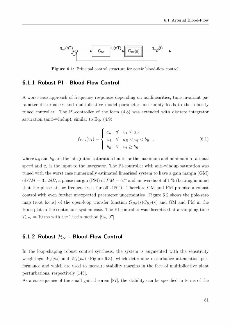
6.1 Arterial Blood-Flow
G (s)BF
u(nT) q (t)aort
+CBF_
q (nT)ref
Figure 6.1: Principal control structure for aortic blood-flow control.
6.1.1 Robust PI - Blood-Flow Control
A worst-case approach of frequency responses depending on nonlinearities, time invariant pa-
rameter disturbances and multiplicative model parameter uncertainty leads to the robustly
tuned controller. The PI-controller of the form (4.8) was extended with discrete integrator
saturation (anti-windup), similar to Eq. (4.9)
fPI,s(uI) =
aR ∀ uI ≤ aR
uI ∀ aR < uI < bR
bR ∀ uI ≥ bR
, (6.1)
where aR and bR are the integration saturation limits for the maximum and minimum rotational
speed and uI is the input to the integrator. The PI-controller with anti-windup saturation was
tuned with the worst case numerically estimated linearised system to have a gain margin (GM)
of GM = 31.2dB, a phase margin (PM) of PM = 57 and an overshoot of 1 % (bearing in mind
that the phase at low frequencies is far off -180). Therefore GM and PM promise a robust
control with even further unexpected parameter uncertainties. Figure 6.2 shows the pole-zero
map (root locus) of the open-loop transfer function GBF (s)CBF (s) and GM and PM in the
Bode-plot in the continuous system case. The PI-controller was discretised at a sampling time
Ts,PI = 10 ms with the Tustin-method [94, 97].
6.1.2 Robust H∞ - Blood-Flow Control
In the loop-shaping robust control synthesis, the system is augmented with the sensitivity
weightings W1(jω) and W3(jω) (Figure 6.3), which determine disturbance attenuation per-
formance and which are used to measure stability margins in the face of multiplicative plant
perturbations, respectively [145].
As a consequence of the small gain theorem [87], the stability can be specified in terms of the
81

6 Control Design
-2000 -1000 0 1000
-2000
-1500
-1000
-500
0
500
1000
1500
2000
2500
real axis
imag axis
-40
-20
0
20
40
60
80magnitude [dB]
10-2
10-1
100
101
102
103
104
-225
-180
-155
-90
frequency [rad/s]
phase [deg]
GM
PM
Figure 6.2: Root locus of the open-loop compensated system GBF (s)C(s).
control system with the frequency-dependent weights, via the inequalities
|S(jω)W1(jω)| < 1
|T (jω)W3(jω)| < 1(6.2)
with the corresponding sensitivity functions
S(jω) =1
GBF (jω)CBF (jω) + 1
T (jω) =GBF (jω)CBF (jω)
GBF (jω)CBF (jω) + 1
(6.3)
In Eq. (6.3) S(jω) determines the disturbance attenuation. T (jω) is used to measure multi-
plicative plant uncertainty [53, 87]. With the sensitivity functions (6.3), the closed-loop transfer
function matrix for the augmented plant, Figure 6.3, leads to the mixed-sensitivity weighted
cost function
GY1,3U1 =
[W1(jω)S(jω)
W3(jω)T (jω)
]. (6.4)
82

6.1 Arterial Blood-Flow
U (jw)1
Y (jw)1
Y (jw)3
C (jw)BF
G (jw)BF
E(jw) Y(jw)
U (jw)2
W (jw)3
W (jw)1
Figure 6.3: Augmented system for robust control.
This in turn leads to the H∞-norm control problem, which is to find a stabilising controller
C(jω), such that the closed-loop controller satisfies the inequality
‖GY1,3U1(jω)‖∞ = supω∈R
|GY1,3U1(jω)| < 1. (6.5)
A 7th orderH∞-controller was calculated using MATLAB’s ’Robust Control Toolbox’ numerical
solution routines and was tuned with the frequency weightings for the ’worst case’ linearised
augmented system (4.24) with applied disturbances and parameter uncertainties, [71, 143, 144].
To guarantee a fast disturbance attenuation, setpoint tracking and no steady-state error, the
frequency-dependent weight W1(jω) was fitted with integral gain and a relatively high corner
frequency. W3(jω) was adjusted to match the suggested multiplicative uncertainty, and is
shown with the system (4.24) in Figure 6.4 [94, 97]. Note that for robust control a small upper
boundary for uncertainties was added to the ’worst case’ linearised system of Eq. (4.24) to
determine W3(jω). The controller was finally discretised at a sampling time of Ts1 = 10 ms.
6.1.3 Adaptive Control
Self-tuning and adaptive control may be described in two ways: As an adaption or an automatic
tuning mechanism [134]. Basically, self-tuning refers to the idea of an initial controller tuning,
an algorithm which is switched off afterwards. In contrast to that, in an adaptive system,
83

6 Control Design
40
30
20
10
0
-10
-20
-30
-40103102100 101
frequencyrads
w (j )1 ω
T(j )ω
S(j )ω
w (j )3 ω
magnitude [dB]
Figure 6.4: Sensitivity functions for robust blood-flow control stability and performance specificationwith frequency-dependent weightings.
a continuous method is used for adjustment of control to varying system parameters. The
control structure considered here is different to model reference adaptive control (MRAC) or
expert tuning systems and is the automatic adjustment of control by estimation of the system
parameters (which are of course expected to vary). This adaptive control structure is sometimes
referred to as self-tuning control and is shown in Figure 6.5.
The control system of Figure 6.5 is divided into a parameter estimation routine and a predictive
controller. The parameter estimation routine (for example a recursive least squares (RLS)
algorithm, or a Kalman Filter (KF)) estimates the system parameters at each sampling step
and updates the controller with the new parameter data. The estimation routine should have the
ability to suppress noise disturbances, that is by the use of a priori noise information, and should
be able to handle slight nonlinearities and time-varying parameters. As the second part of the
discrete adaptive control system, the control algorithm is updated at every sampling instant
with new parameter information, provided by the parameter estimation routine. A general
predictive control (GPC) algorithm in turn generates a control signal from the past control
input, system output and parameter data. This adaptive control approach has the advantage
of operating under the conditions of uncertainty, that is, unknown system parameters. The
characteristics of the plant are to be found to which the system can adapt itself on-line.
84

6.1 Arterial Blood-Flow
Plant
Measurementnoiseu(nT )s
G (s)BF
y(t)
TsTsTs
Estimation routine(e.g. KF)
Parameter vector
Adaptivecontrol (GPC)
y(nT)
r(nT)
Figure 6.5: Structure of the adaptive control system.
Kalman Filter Implementation
As the base of the estimation routine, an autoregressive moving average model with exogenous
input (ARMAX) was used as the estimation model [93]
A(q−1)y(k) = q−mB(q−1)u(k) + C(q−1)ν(k), (6.6)
where u(k) is the input and y(k) is the output. ν(k) is assumed to be a white noise sequence
(average mean of zero) with constant known variance
µ = Eν = 0
σ2 = E(ν − µ)2.(6.7)
The polynomials for (6.6) are defined as
A(q−1) = 1 + a1q−1 + a2q
−2 + ... + anaq−na
B(q−1) = b0 + b1q−1 + b2q
−2 + ... + bnbq−nb ,
C(q−1) = 1 + c1q−1 + c2q
−2 + ... + cncq−nc
(6.8)
85

6 Control Design
with na ≥ nb, b0 6= 0, m > 1 and q−1 the backward shift operator [93]. Eq. (6.6) is rearranged
with the parameter vector
θ = [a1 a2 ... ana ; b0 b1 ... bnb]T (6.9)
and the observation vector
χ(k) = [−y(k− 1) − y(k− 2) ... − y(k−na); u(k−m) u(k−m− 1) ... u(k−m−nb)]. (6.10)
Substituting Eqs. (6.9) and (6.10) into (6.6) gives
y(k) = χ(k)θ + ε(k)
ε(k) = C(q−1)ν(k).(6.11)
In further considerations, the noise colouring polynomial C(q−1) is assumed to be one. Therefore
Eq. (6.11) simplifies to
y(k) = χ(k)θ + ν(k). (6.12)
The parameter estimating KF equations for (6.12) were obtained from the well-known KF
observer equations by making the transition for state vector x → θ and output mapping c → χ,
[59, 60, 72]. Recursive KF equations are separated in a prediction and a correction phase.
Prediction:
θ(k|k − 1) = θ(k − 1|k − 1)
Φ(k|k − 1) = Φ(k − 1|k − 1) + Rw
(6.13)
Correction:
θ(k|k) = θ(k|k − 1) + φ(k)[y(k)− χ(k)θ(k|k − 1)]
φ(k) = Φ(k|k − 1)χT (k)[rv + χ(k)Φ(k|k − 1)χT ]−1,
Φ(k|k) = [I− φ(k)χ(k)]Φ(k|k − 1)
(6.14)
where θ(k|k − 1) is the estimated parameter vector, rv is the noise variance, Rw is the process
noise covariance matrix, Φ is the covariance matrix, φ is the Kalman gain vector, and I is
the identity matrix (all of appropriate dimensions). The notation θ(k|k − 1) indicates the
parameter estimate at time k, based on information of and up to k− 1. Eqs. (6.13) and (6.14)
are implemented for online estimation of the parameters of a second order system.
86

6.2 Arterial Pressure Control
General Predictive Control
The GPC controller is designed and tuned using the general minimum variance cost function
law with integral control action ∆u(k) = u(k)− u(k − 1) [26].
JGPC = Emin
hp∑
j=kc
[y(k + j)− r(k + j)]2 +hc∑
j=1
[φGPC∆u(k + j − 1)]2
(6.15)
with control delay kc, prediction and control horizon hp and hc and φGPC is the control input
cost weighting. There are two terms in the cost function (6.15) that are to be minimised for the
controller. The first term is future deviations of the system output to the control set point and
the second term is the variance of future incremental control action. The incremental control
cost can thereby be ’tuned’ by the weighting φGPC . Minimising the GPC cost function (6.15)
leads to the GPC controller [26], based on the ARMAX model (6.12). The GPC controller is
updated with estimated parameters at each sampling instance and is therefore self-tuning.
For simulation and experimental implementation, the sampling time Ts2 = 100 ms of the system
was chosen to fit the time-delay. For parameter estimation, second order dynamics na = 2,
nb = 1 were assumed in the KF, which gave the best results in control experiments. Since
a linear prediction series in a nonlinear system may lead to errors, the prediction horizon hc
was chosen to hc = 1. The time series of future control reference values was assumed to be
unknown, therefore hp = 1. Another reason for the short prediction horizon are the system
inherent nonlinear characteristics, to which the self-tuning routine has to adapt (to prevent
system prediction errors due to nonlinearities, not predicted in the recursive prediction).
6.2 Arterial Pressure Control
6.2.1 Total Arterial Pressure Control
Similar to arterial blood-flow control, the arterial pressure was fed back and compared to the
pressure setpoint to form the error as input for control, see Figure 6.6. With regard to the
model, this means that the aortic pressure of the first vascular compartment is used. Eq.
(4.24) was only changed in terms of the output mapping vector c.
Note that during CPB a direct aortic pressure measurement is in most cases not available.
87

6 Control Design
Pressure is measured in certain arteries and therefore subject to error, depending on the vascular
system. In Section 4.3 the flow pressure curve of the aortic cannula was shown to have a
quadratic behaviour (Figure 5.4). Therefore, the measured pressure has to be corrected by
the cannula curve, corresponding to the tip diameter of the cannula. According to (4.10), the
pressure drop over the cannula ∆pC is dependent on blood-flow
∆pC = qbRC(qB). (6.16)
With this pressure drop over the cannula, the measured pre-cannula pressure was then corrected
to the aortic pressure
paort = part −∆pC , (6.17)
see pressure correction (PC) block (Figure 6.6). For the tuning of a PI-controller, the model
(4.24) with aortic pressure output was linearised in the same way as in Section 6.1.1. The
resulting linear TF is
GBPC(s) =Paort(s)
Uin(s), (6.18)
where in the linearisation process a constant value for vasoactive drug injection (using Propofol
as one of the most influencing substances) is used. With the root-locus method [71, 94], a
PI-controller of the form (4.6) - (4.9) was tuned with the worst case linearised model to have a
gain margin of GM = 17.9 dB and a phase margin of PM = 66.3. Figure 6.7 shows the root
locus-plot, together with the Bode-Plot of the open-loop compensated system (C(s)GBPC(s)).
Control G (s)BP
u(nT) p (t)artp (nT)ref
+_
PCp (t)aort
Figure 6.6: Total arterial pressure control with pressure correction (PC) in the feedback-loop.
6.2.2 Arterial Pressure Boundary Control
To keep the mean arterial pressure (MAP) within boundaries 40-60 mmHg (see Section 4.1) a
cascaded control structure was developed, which adjusts the mean blood-flow control reference
88
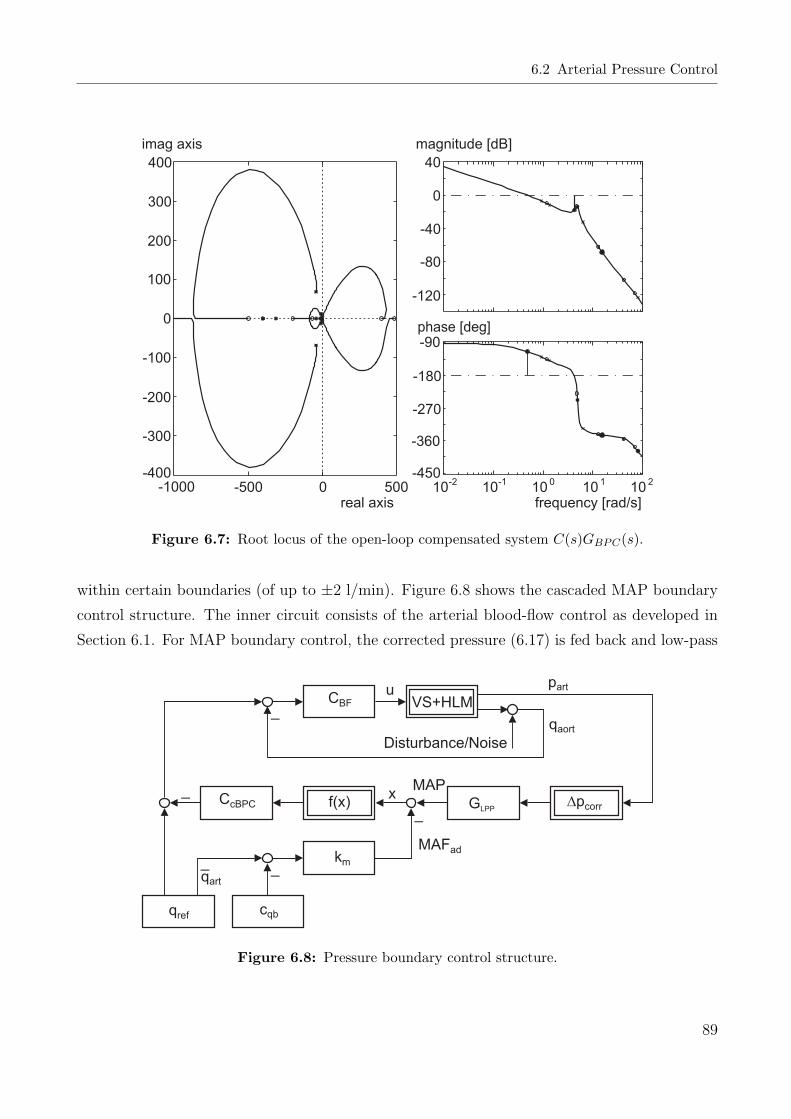
6.2 Arterial Pressure Control
-1000 -500 0 500-400
-300
-200
-100
0
100
200
300
400
real axis
imag axis
-120
-80
-40
0
40
magnitude [dB]
10-2
10-1
100
101
102
-450
-360
-270
-180
-90
frequency [rad/s]
phase [deg]
Figure 6.7: Root locus of the open-loop compensated system C(s)GBPC(s).
within certain boundaries (of up to ±2 l/min). Figure 6.8 shows the cascaded MAP boundary
control structure. The inner circuit consists of the arterial blood-flow control as developed in
Section 6.1. For MAP boundary control, the corrected pressure (6.17) is fed back and low-pass
Disturbance/Noise
f(x) GLPP
qaort
km
VS+HLM
_
_
_
_
upart
qart
_
Dpcorr
CBF
CcBPC
cqbqref
MAFad
xMAP
Figure 6.8: Pressure boundary control structure.
89

6 Control Design
filtered, by a filter of the form
GLPP (s) =MAP (s)
paort(s)=
1
TLPP s + 1. (6.19)
The MAP is then compared with the reference mean arterial pressure (MAFad), determined
from the flow operating point by the linear function
MAFad = kqb(qart − cqb), (6.20)
in which kqb is a gain and cqb is a constant, both determined to fit mean arterial flow to mean
arterial pressure. A function f(x) maps the absolute difference pcorr = x = MAP - MAFad to
an control error ep (Figure 6.9). Function f(x) is a hyperbolic weighting of the form
f(x) =1
kg
sinh(x− cg), (6.21)
with the gain kg and the normal operating-point for pressure cg, at which the control input error
goes to zero. Eqs. (6.16) - (6.21) were combined with a PI-controller CcBPC(s) of the form (4.6)
- (4.9), which was tuned with the worst case linearised model of the closed arterial blood-flow
circuit to have a gain margin of GM = 17.3 dB and a phase margin PM = 54. Figure 6.10
shows the root-locus plot, together with the Bode-Plot of the open-loop compensated system
(CcBPC(s)GcBFC(s)), in which GcBFC is the closed blood-flow control circuit.
20 30 40 50 60 70 80-20
-15
-10
-5
0
5
10
15
20
e [ ] = f (x)pw
p [mmHg] = xcorr
Figure 6.9: Mean arterial pressure difference mapping to a control error.
90

6.3 Blood-Gas
-2000 -1000 0 1000 2000-2000
-1500
-1000
-500
0
500
1000
1500
2000
real axis
imag axis
-100
-50
0
50
magnitude [dB]
10-2
10-1
100
101
102
-225
-180
-135
-90
-45
frequency [rad/s]
phase [deg]
Figure 6.10: Root locus of the open-loop compensated system C(s)GcBFC(s).
6.3 Blood-Gas
’Fortunately’ in physiological terms the transport of blood-gases in the human body is by
itself a highly nonlinear process. This nonlinear behaviour together with other physiological
control mechanisms prevents the body from under- or over oxygenation and keeps the carbon
dioxide content and the affiliated pH-values within normal ranges in physiological conditions.
’Unfortunately’ in control engineering terms the artificial blood-gas circuit includes a number
of properties, complicating the development of control algorithms, such as
a) nonlinearities, which are mainly oxygen saturation and flow dependent dynamics and
result in process gain changes of 700 % and above,
b) uncertainties, for example the haemoglobin content of the blood, which depends on blood
priming and determines the binding capacities of oxygen and carbon dioxide and therefore
model gains (note that the haemoglobin content is measurable online during CPB),
c) time-varying parameters, for example the clotting of blood in the oxygenator and the
91

6 Control Design
resulting reduction of the diffusion capacities (and therefore process gain) with time,
d) flow and tubing system dependent time-delays, which can vary up to and over 300 %.
Since classic linear feedback control theory performs only suboptimally on uncertain nonlinear
systems incorporating time-varying process characteristics and time-delays and therefore cannot
guarantee global stability, modern robust nonlinear control theory will be needed. A controller
for feedback control of blood-gases has to guarantee robust stability and performance under
the above-named system properties. The control approach, developed in this work, is described
below.
The Smith-predictor, as proposed in the 1950s [120], can improve the close-loop performance
of linear systems incorporating time-delays. However, special care has to be taken in Smith-
predictor design if performance and disturbance rejection in the closed-loop control circuit facing
uncertainties in the form of modelling errors is of concern. The Smith-predictor structure relates
to the internal model control (IMC) structure, which in turn offers performance advantages by
addressing the robustness problem explicitly [87]. With the help of modern geometric theory
of nonlinear control a large class of nonlinear systems can be linearised by a nonlinear state
feedback control law [44, 55, 56, 110]. In this way, the Smith-predictor structure can be extended
to this class of nonlinear systems by the use of open-loop observers (similar to IMC). By adding
an external linear controller, the linearised system compensated for time-delay can be made
robust with respect to time-delay errors and uncertainties [66].
The structure for blood-gas control can be divided into oxygen partial pressure pO2- and carbon
dioxide partial pressure pCO2-control. Figure 6.11 shows the structure of the suggested O2-
controller with Smith-predictor and open-loop state observer, linearisation by state feedback
Ψ(·) and external linear controller. The figure shows also the process input values gas flow
qg, blood-flow qb and oxygen fraction FiO2. Note that the process gain of the linearised plant
still varies with blood-flow qb, which can be seen as a predictable disturbance. The external
O2-controller is therefore gain-scheduled depending on blood-flow qb.
The process characteristics for pCO2-plant and controller are not so critical. An adaptive gain
controller, dependent on arterial blood-flow qb, as seen in Figure 6.12 was used for pCO2-control.
The structure of this section is as follows. First, the model of Eqs. (4.30) - (4.48) is substituted
to a suitable nonlinear affine state space model. After feedback linearisation the external linear
(pO2) controller and the adaptive gain (pCO2) controller are developed. The section ends up
with simulation results for setpoint tracking and disturbance rejection performance.
92
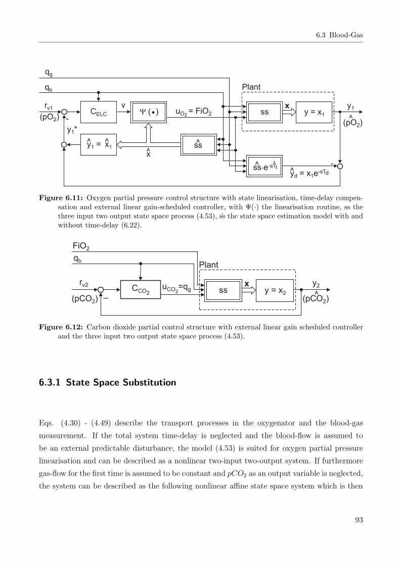
6.3 Blood-Gas
Y ( )•
x
-
-
CELC
rv1
y = x11
xss
ss.e-s^Tt
ssu = FiOO 22 y = x1
y1
y = x ed 1-sTd
Plant
v
qg
qb
(pO )2(pO )2
^
y *1
Figure 6.11: Oxygen partial pressure control structure with state linearisation, time-delay compen-sation and external linear gain-scheduled controller, with Ψ(·) the linearisation routine, ss thethree input two output state space process (4.53), ss the state space estimation model with andwithout time-delay (6.22).
CCO2u =qCO g2
y2rv2
qb
_(pCO )2 (pCO )2
FiO2
xss y = x2 ^
Plant
Figure 6.12: Carbon dioxide partial control structure with external linear gain scheduled controllerand the three input two output state space process (4.53).
6.3.1 State Space Substitution
Eqs. (4.30) - (4.49) describe the transport processes in the oxygenator and the blood-gas
measurement. If the total system time-delay is neglected and the blood-flow is assumed to
be an external predictable disturbance, the model (4.53) is suited for oxygen partial pressure
linearisation and can be described as a nonlinear two-input two-output system. If furthermore
gas-flow for the first time is assumed to be constant and pCO2 as an output variable is neglected,
the system can be described as the following nonlinear affine state space system which is then
93
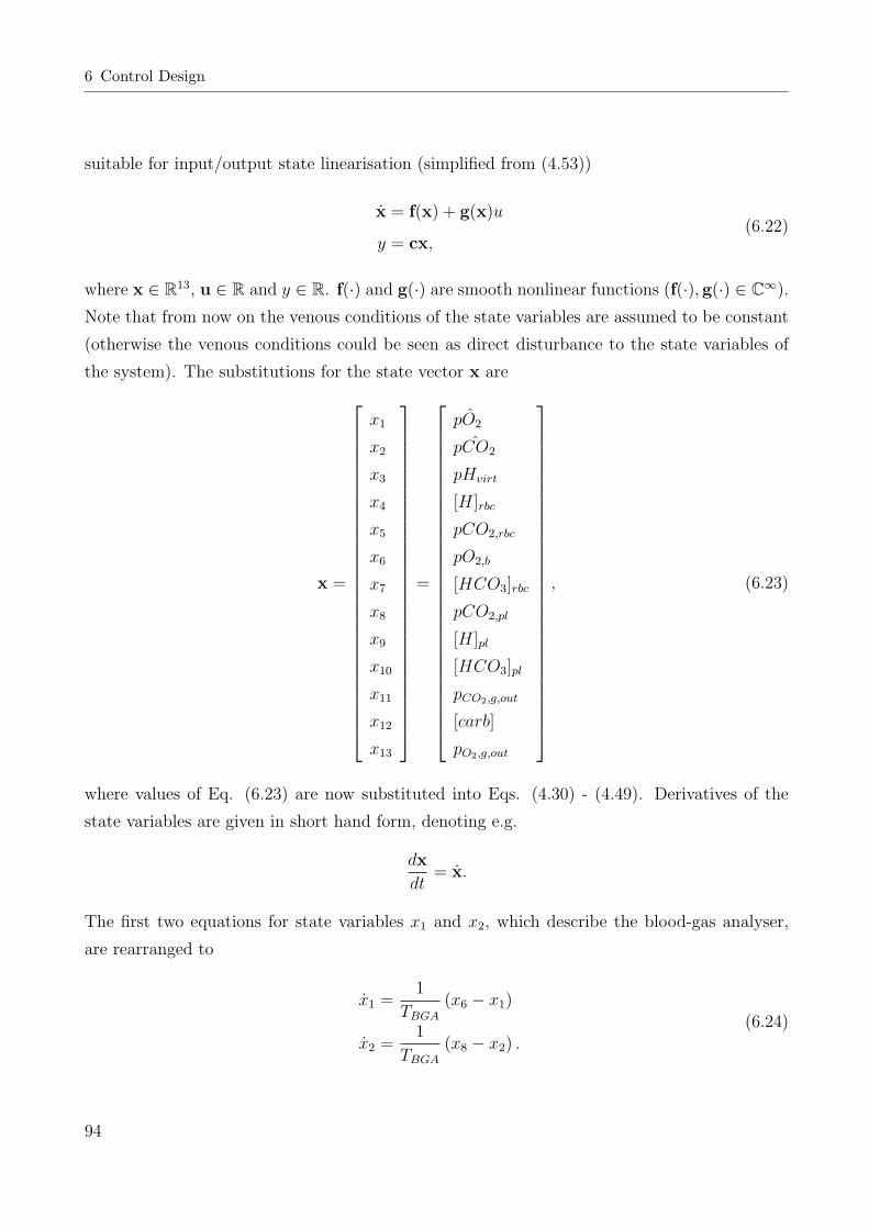
6 Control Design
suitable for input/output state linearisation (simplified from (4.53))
x = f(x) + g(x)u
y = cx,(6.22)
where x ∈ R13, u ∈ R and y ∈ R. f(·) and g(·) are smooth nonlinear functions (f(·),g(·) ∈ C∞).
Note that from now on the venous conditions of the state variables are assumed to be constant
(otherwise the venous conditions could be seen as direct disturbance to the state variables of
the system). The substitutions for the state vector x are
x =
x1
x2
x3
x4
x5
x6
x7
x8
x9
x10
x11
x12
x13
=
pO2
pCO2
pHvirt
[H]rbc
pCO2,rbc
pO2,b
[HCO3]rbc
pCO2,pl
[H]pl
[HCO3]pl
pCO2,g,out
[carb]
pO2,g,out
, (6.23)
where values of Eq. (6.23) are now substituted into Eqs. (4.30) - (4.49). Derivatives of the
state variables are given in short hand form, denoting e.g.
dx
dt= x.
The first two equations for state variables x1 and x2, which describe the blood-gas analyser,
are rearranged to
x1 =1
TBGA
(x6 − x1)
x2 =1
TBGA
(x8 − x2) .(6.24)
94

6.3 Blood-Gas
Eqs. (4.30) - (4.48) become now, sorted in state order
x3 =1
TpH
[−x3 − log (x4 ((0.058x3 − 0.437) S(xx)− 0.529x3 + 4.6))]
x4 =1
Vrbc
[qrbc ([H]rbc,in − x4)− Vrbc
2.303
βrbc
x4
(−RHCO3,rbc + 1.5x12 − 0.6capS(xx)
) ]
x5 =1
αCO2Vrbc
[qrbc ([CO2]rbc,in − αCO2x5) + DCO2,m(x8 − x5) + VrbcRHCO3,rbc − Vrbcx12
]
x6 =qb ([O2]b,in − [O2]b) + DO2,m(x13 − x6)
Vb
(αO2 + capb
dS(xx)dxx
dxx
x6
)
x7 =1
Vrbc
[qrbc ([HCO3]rbc,in − x7) + DHCO3,rbc
(x10 − x7
r
)− VrbcRHCO3,rbc
]
x8 =1
VplαCO2
[qpl ([CO2]pl,in − αCO2x8) +
DCO2,m(x11 − x8) + DCO2,rbc(x5 − x8) + VplRHCO3,pl
]
x9 =1
Vpl
[qpl ([H]pl,in − x9)− Vpl
2.303
βrbc
x9RHCO3,pl
]
x10 =1
Vpl
[qpl ([HCO3]pl,in − x10)−DHCO3,rbc
(x10 − x7
r
)− VplRHCO3,pl
]
x11 =1
Vg
(qg(pCO2,g,in − x11) + DCO2,mpbar(x8 − x11)
)
x12 =1
Vrbc
[qrbc ([carb]in − x12) +
kaαCO2Vrbcx5([Hb]− x12)
(kzoS(xx)
kzo + x4
+kzr(1− S(xx))
kzr + x4
)− Vrbc
kax12x4
kc
]
x13 =1
Vg
(qg(pO2,g,in − x13) + DO2,mpbar(x6 − x13)
).
(6.25)
Note that the state equation for x3 is rearranged from Eqs. (4.43) and (4.44). The state
equation for the Eqs. (4.43), (4.44) is introduced because of simulation problems with the
algebraic loop. The new time constant TpH is introduced to keep the transient responses of
state equation x3 as minimal as possible with the goal of avoiding a stiff system at the same
time.
95
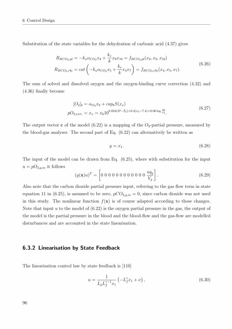
6 Control Design
Substitution of the state variables for the dehydration of carbonic acid (4.37) gives
RHCO3,pl = −kuαCO2x8 +kv
kx9x10 = fHCO3,pl(x8, x9, x10)
RHCO3,rbc = cat
(−kuαCO2x5 +
kv
kx4x7
)= fHCO3,rbc(x4, x5, x7).
(6.26)
The sum of solved and dissolved oxygen and the oxygen-binding curve correction (4.32) and
(4.36) finally become
[O2]b = αO2x6 + capbS(xx)
pO2,virt. = xx = x6100.024(37−Tb)+0.4(x3−7.4)+0.06 log 40
x5 .(6.27)
The output vector c of the model (6.22) is a mapping of the O2-partial pressure, measured by
the blood-gas analyser. The second part of Eq. (6.22) can alternatively be written as
y = x1. (6.28)
The input of the model can be drawn from Eq. (6.25), where with substitution for the input
u = pO2,g,in it follows
(g(x)u)T =
[0 0 0 0 0 0 0 0 0 0 0 0
uqg
Vg
]. (6.29)
Also note that the carbon dioxide partial pressure input, referring to the gas flow term in state
equation 11 in (6.25), is assumed to be zero, pCO2,g,in = 0, since carbon dioxide was not used
in this study. The nonlinear function f(x) is of course adapted according to those changes.
Note that input u to the model of (6.22) is the oxygen partial pressure in the gas, the output of
the model is the partial pressure in the blood and the blood-flow and the gas-flow are modelled
disturbances and are accounted in the state linearisation.
6.3.2 Linearisation by State Feedback
The linearisation control law by state feedback is [110]
u =1
LgLγ−1f x1
(−Lγfx1 + ν
), (6.30)
96

6.3 Blood-Gas
where Lfx1 and LgLfx1 are the Lie-differentials defined by
Lfx1 =∂x1
∂xf(x)
LgLfx1 =∂x1
∂xg(x).
(6.31)
The linearisation procedure can be described as to differentiate the system output y until the
system input u appears in the term LgLγ−1f x1 and is bounded away from zero for all x ∈ U ,
where U is an open subset of R13, containing the equilibrium point of the undriven system x0.
The linearised system is then the γth order linear system from the new substituted input ν to
the output y.dγy
dtγ= ν (6.32)
(with the strict relative degree γ, [110]).
If the system of (6.22) has stable zero dynamics and (6.22) has the strict relative degree γ, the
state feedback law [19, 110]
u =1
LgLγ−1f x1
(−
γ∑j=0
βjLjfx1 + ν
)(6.33)
with the polynomial
sγ + βγ−1sγ−1 + · · ·+ β1s + β0, βγ = 1 (6.34)
which makes the system of (6.22) exponentially stable. The polynomial (6.34) is assumed to
be Hurwitz, i.e. has real positive coefficients and roots which are either negative or pairwise
conjugate with negative real parts. The (locally) exponential stable linear system yields
γ∑j=0
βjy(j) = ν. (6.35)
Note that the coefficients βj, j = 0 . . . γ cannot be chosen arbitrarily, as can the time constant
of the asymptotically linearised system. Special care has to be taken of input saturation and
sampling-time.
For the linearisation law for asymptotic stabilisation (6.35), the Lie-differentials LgLγ−1f x1 and
Ljfx1 up to j = γ are needed. This procedure with respect to the blood-gas system is described
97

6 Control Design
below. Differentiating the system output of equation
x = f(x) + g(x)u
y = x1,(6.36)
with respect to time yields
dy
dt= y =
∂x1
∂xf(x) +
∂x1
∂xg(x)u, (6.37)
where∂x1
∂x= [1 0 0 0 0 0 0 0 0 0 0 0 0] . (6.38)
Expansion of Eq. (6.37) leads to
y =1
TBGA
(x6 − x1) . (6.39)
The second term in Eq. (6.37) corresponding to the input is zero. Therefore, further differen-
tiating of the output y gives
dy
dt= y =
∂Lfx1
∂xf(x) +
∂Lfx1
∂xg(x)u
= L2fx1 + LgLfx1u,
(6.40)
where
∂Lfx1
∂x=
∂ 1TBGA
(x6 − x1)
∂x
=
[− 1
TBGA
0 0 0 01
TBGA
0 0 0 0 0 0 0
].
(6.41)
Incorporating (6.41) into (6.24)-(6.25) results in
L2fx1 =
[− 1
TBGA
0 0 0 01
TBGA
0 0 0 0 0 0 0
]f(x)
=1
TBGA
1
TBGA
(x1 − x6) +qb ([O2]b,in − [O2]b) + DO2,m(x13 − x6)
Vb
(αO2 + capb
dS(xx)dxx
dxx
x6
) .
(6.42)
98

6.3 Blood-Gas
Since the second term of Eq. (6.40) LfLgx1 is zero, Eqs. (6.40) and (6.42) combine to
y =1
TBGA
1
TBGA
(x1 − x6) +qb ([O2]b,in − [O2]b) + DO2,m(x13 − x6)
Vb
(αO2 + capb
dS(xx)dxx
dxx
x6
) . (6.43)
For a third differentiation of the output y and the partial derivative∂L2
f x1
∂x, a few prerequisites
have to be made:
For the differentiation of the oxygen saturation curve (4.35), numerator and denominator are
Sn(xx) = a1xx + a2x2x + a3x
3x + x4
x
Sd(xx) = a4 + a5xx + a6x2x + a7x
3x + x4
x.(6.44)
Differentiation with respect to xx gives
dSn(xx)
dxx
= a1 + 2a2xx + 3a3x2x + 4x3
x
d2Sn(xx)
dx2x
= 2a2 + 6a3xx + 12x2x,
(6.45)
and
dSd(xx)
dxx
= a5 + 2a6xx + 3a7x2x + 4x3
x
d2Sd(xx)
dx2x
= 2a6 + 6a7xx + 12x2x.
(6.46)
Further needed is the squared denominator polynomial
S2d(xx) =
(a4 + a5xx + a6x
2x + a7x
3x + x4
x
) (a4 + a5xx + a6x
2x + a7x
3x + x4
x
)
= a4 + a4a5xx + a4a6x2x + a4a7x
3x + a4x
4x
+ a4a5xx + a25x
2x + a5a6x
3x + a5a7x
4x + a5x
5x
+ a4a6x2x + a5a6x
3x + a2
6x4x + a6a7x
5x + a6x
6x
+ a4a7x3x + a5a7x
4x + a6a7x
5x + a2
7x6x + a7x
7x
+ a4x4x + a5x
5x + a6x
6x + a7x
7x + x8
x
= a4 + 2a4a5xx + (2a4a6 + a25)x
2x + 2(a4a7 + a5a6)x
3x + (2a4 + 2a5a7 + a2
6)x4x
+ 2(a5 + a6a7)x5x + (2a6 + a2
7)x6x + 2a7x
7x + x8
x
(6.47)
99

6 Control Design
and its differentiation
dS2d(xx)
dxx
= 2a4a5 + 2(2a4a6 + a25)xx + 6(a4a7 + a5a6)x
2x + 4(2a4 + 2a5a7 + a2
6)x3x
+ 10(a5 + a6a7)x4x + 6(2a6 + a2
7)x5x + 14a7x
6x + 8x7
x.
(6.48)
From Eqs. (6.44)-(6.48) and Eq. (4.35) result the differentiation for Eq. (4.35) to
dS(xx)
dxx
=S ′n(xx)Sd(xx)− Sn(xx)S
′d(xx)
S2d(xx)
, (6.49)
where S ′(xx) = dS(xx)dxx
. Differentiating (6.49) a second time, results in
d2S(xx)
dx2x
= [S ′′n(xx)Sd(xx) + S ′n(xx)S′d(xx)− Sn(xx)S
′′d (xx)− S ′n(xx)S
′d(xx)] S
2d(xx)
− [S ′n(xx)Sd(xx)− Sn(xx)S′d(xx)]
dS2d(xx)
dxx
1
S4d(xx)
=[S ′′n(xx)Sd(xx)− Sn(xx)S
′′d (xx)] S
2d(xx)− [S ′n(xx)Sd(xx)− Sn(xx)S
′d(xx)]
dS2d(xx)
dxx
S4d(xx)
.
(6.50)
Further prerequisites for the partial differential∂L2
f x1
∂xare the inner derivatives of the oxygen
saturation curve (4.35), which apply to the pO2-correction Eq. (4.36)
∂xx
∂x3
= 0.4 ln(10)x6100.024(37−Tb)+0.4(pHvirt−7.4)+0.06 log 40
pCO2
∂xx
∂x5
= −0.06x6
x5
100.024(37−Tb)+0.4(pHvirt−7.4)+0.06 log 40
pCO2
∂xx
∂x6
= 100.024(37−Tb)+0.4(pHvirt−7.4)+0.06 log 40
pCO2 ,
(6.51)
and
∂
∂x3
(∂xx
∂x6
)= 0.4 ln(10)10
0.024(37−Tb)+0.4(pHvirt−7.4)+0.06 log 40pCO2
∂
∂x5
(∂xx
∂x6
)= −0.06
1
x5
100.024(37−Tb)+0.4(pHvirt−7.4)+0.06 log 40
pCO2 .
(6.52)
100

6.3 Blood-Gas
The derivation of the oxygenation saturation curve derivative with respect to the state variables
x3, x5 and x6 is for j = 3, 5, 6
∂
∂xj
(∂S(xx)
∂xx
)=
∂S2(xx)
∂x2x
∂xx
∂xj
(6.53)
Using Eqs. (6.44)-(6.53), the different terms for the partial derivative∂L2
f x1
∂xare
∂L2fx1
∂x2
=∂L2
fx1
∂x4
=∂L2
fx1
∂x7
=∂L2
fx1
∂x8
=∂L2
fx1
∂x9
=∂L2
fx1
∂x10
=∂L2
fx1
∂x11
=∂L2
fx1
∂x12
= 0, (6.54)
∂L2fx1
∂x3
=∂
∂x3
fz︷ ︸︸ ︷qb ([O2]b,in − [O2]b) + DO2,m(x13 − x6)
TBGAVb
(αO2 + capb
dS(xx)
dxx
dxx
dx6
)
︸ ︷︷ ︸fn
=∂
∂x3
fz
fn
=−qbcap∂S(xx)
∂xx
∂xx
∂x3fn − TBGAVbcap ∂
∂x3
(∂S(xx)
∂xx
)∂
∂x3
(∂xx
∂x6
)fz
f 2n
∂L2fx1
∂x5
=∂
∂x5
fz︷ ︸︸ ︷qb ([O2]b,in − [O2]b) + DO2,m(x13 − x6)
TBGAVb
(αO2 + capb
dS(xx)
dxx
dxx
dx6
)
︸ ︷︷ ︸fn
=∂
∂x5
fz
fn
=−qbcap∂S(xx)
∂xx
∂xx
∂x5fn − TBGAVbcap ∂
∂x5
(∂S(xx)
∂xx
)∂
∂x5
(∂xx
∂x6
)fz
f 2n
∂L2fx1
∂x6
= − 1
T 2BGA
+∂
∂x6
fz︷ ︸︸ ︷qb ([O2]b,in − [O2]b) + DO2,m(x13 − x6)
TBGAVb
(αO2 + capb
dS(xx)
dxx
dxx
dx6
)
︸ ︷︷ ︸fn
= − 1
T 2BGA
+∂
∂x6
fz
fn
= − 1
T 2BGA
+
[(−qb
(cap
∂S(xx)
∂xx
∂xx
∂x6
+ αO2
)−DO2,m
)fn
− TBGAVbcap∂
∂x6
(∂S(xx)
∂xx
)∂xx
∂x6
fz
]1
f 2n
,
(6.55)
101

6 Control Design
and
∂L2fx1
∂x1
=1
T 2BGA
∂L2fx1
∂x13
=DO2,m
Vb
(αO2 + capb
dS(xx)dxx
dxx
x6
) .(6.56)
From equation (6.54)-(6.56) follows
∂L2fx1
∂x=
[∂L2
fx1
∂x1
0∂L2
fx1
∂x3
0∂L2
fx1
∂x5
∂L2fx1
∂x6
0 0 0 0 0 0∂L2
fx1
∂x13
](6.57)
and∂L2
fx1
∂xf(x) = L3
fx1. (6.58)
The Lie-derivative with respect to the input is
∂L2fx1
∂xg(x) = LgL
2fx1 =
DO2,m
qg
Vg
Vb
(αO2 + capb
dS(xx)dxx
dxx
x6
) , (6.59)
where during linearising control a gas flow of qg → 0 has to be prevented to guarantee the relative
degree γ = 3 (see Eq. (6.30)). This design issue is of special importance when designing the
pCO2-controller, which uses the gas flow qg as the control input. With
d3y
dt3=
∂L2fx1
∂xf(x) +
∂L2fx1
∂xg(x)u,
= L3fx1 + LgL
2fx1u,
(6.60)
follows the linearising feedback law to
u =1
LgL2fx1
(−
3∑j=0
βjLjfx1 + ν
), (6.61)
with
LgL2fx1 6= 0 ∀ x ∈ U . (6.62)
The parameters β0 . . . β3 were adapted to the input constraints and sampling time Ts,BGA =
6 s of system (6.36) such that the closed-loop asymptotic linearised system’s time constant is
102

6.3 Blood-Gas
placed at the triple pole p1,2,3 = 0.25 (see Appendix B). Figure 6.13 shows the block diagram
of the linearisation loop, applied to the nonlinear O2-plant with y1 = y as the output.
The linearisation model was implemented together with the nonlinear state-space system in
MATLAB/Simulink and showed asymptotic stabilisation over the whole operating range. However,
for practical implementation the problem of unavailability of the system states remains. There
are two ways to solve this problem guaranteeing robustness of the external linear control (which
is to be applied later).
1. The implementation of a robust discrete (exponential) observer.
2. The implementation of a robust internal model control (IMC) like structure, with the
estimation model as an open-loop state observer.
Since the first approach means additional and unpredictable complexity and calculation cost,
the second approach was chosen for an application. By designing the external linear controller
(ELC) with regard to model and predicted delay-time uncertainty, robustness can be achieved.
6.3.3 Robust External Linear pO2-Controller Design
Following the Smith-predictor structure [120], a Smith-like predictor with linearisation feedback
for asymptotic stabilisation (Section 6.3.2) was combined with the prediction feedback
y∗1 = y1 + (y1 − yd), (6.63)
to form the nonlinear control-loop for the real plant output y1 = ˆpO2, see Figure 6.11. In Eq.
(6.63) y1 is the predicted oxygen partial pressure system output without any time-delay, and
yd is the predicted time-delayed oxygen partial pressure output. An external linear controller
CELC was gain-scheduled in dependance of the blood-flow through the oxygenator. This is
because of the changing linear system gain in dependance of the blood-flow qb.
Y ( )•
v xx f(x) g(x)•
= + u y = x1
y =1u =FiOO 22 ^
pO2^^
Figure 6.13: Linearisation loop (6.61) for the nonlinear O2-plant without time-delay.
103

6 Control Design
The requirements for the external linear controller are robustness and performance in the face of
uncertainties, whether in the degrading plant or the prediction and linearisation routines. In a
first step, uncertainty was assumed for the linearised system (6.35) in the form of unstructured
multiplicative and time-delay uncertainty.
The unstructured multiplicative uncertainty was modelled with the nominal model Glin(s),
which is the linear transfer function, obtained by the state linearisation (see above). The
multiplicative uncertainty was modelled such that
Gp = Glin(s)(1 + lm(s)) (6.64)
describes a member of the family of plants, with lm(s) the unstructured multiplicative uncer-
tainty. The family of plants is then given by
Π =
Gp(s) :
|Gp(s)−Glin(s)||Glin(s)| ≤ lm(ω)
, (6.65)
where lm(ω) ≥ |lm(s)| is the unstructured multiplicative uncertainty bound [87].
Multiplicative uncertainty was assumed in terms of bound lm1(s) and lm2(s). lm1(s) is composed
of uncertainties of the linearisation and the state estimation process and is described by the
’worst case’ transfer function G(s)
G(s) =αw0
βw3s3 + βw2s2 + sβw1 + βw0
, (6.66)
which is the linearised TF with static gain and high frequency gain uncertainty, where it is
assumed that all TFs of the plant family are described by (6.66). Note that the linearised TF
is of third order, because of the relative degree of the linearisation process. Parameters for Eq.
(6.66) are given in Appendix B. The uncertainty lm1(s) follows to
lm1(s) =G(s)−Glin(s)
Glin(s). (6.67)
The multiplicative uncertainty lm2(s) is the error in the time-delay, when neglecting the input
time-delay at the linearisation (which is not large) and other time-delays in the prediction. If
the total time-delay is
Tdt = Td + Tδ (6.68)
104

6.3 Blood-Gas
and composed of total process time-delay Td = Td1 + Td2 and time-delay uncertainty Tδ, the
multiplicative uncertainty can be described as
lm2(s) =e−sTdt − esTd
e−sTd
= e−sTδ − 1.
(6.69)
From Eq. (6.69) follows for the time-delay uncertainty to
|lm2(s)| =
2 sin ωTδ
2∀ ω ≤ π
Tδ
2 ∀ ω ≥ πTδ
.(6.70)
The time-delay uncertainty was modelled with a frequency-bound approximation lm2(s) for
(6.70) of the form
lm2(s) = km2s + αm2
s + βm2
, (6.71)
with constants to be found in Appendix B. The total system multiplicative unstructured
uncertainty is then lumped as
lm(s) = lm1(s) · lm2(s). (6.72)
With the requirement for robust stability, Eq. (6.2) becomes
‖T (jω)lm(jω)‖∞ < 1, (6.73)
where in this case the complementary sensitivity function is
T (jω) =CELC(jω)Glin(jω)
CELC(jω)Glin(jω) + 1, (6.74)
as defined in (6.3).
To determine sufficient disturbance rejection the sensitivity function (6.3)
S(jω) =1
CELC(jω)Glin(jω) + 1, (6.75)
can used, which leads to the nominal performance condition (6.2)
‖S(jω)w1(jω)‖∞ < 1, (6.76)
105

6 Control Design
where w1(s) is the performance weighting function yet to be specified. For integral control with
relatively high corner frequency (-3dB at 0.06 rad/sec), the control performance sensitivity
weighting was chosen to
w1(s) = kp1s + αp1
s. (6.77)
An external linear PI-controller CELC(s) was tuned with the linear system of (6.35) with re-
gard to the nominal performance (6.76) and the robust stability (6.73) condition. Figure 6.14
shows the sensitivity functions with the uncertainty, the performance weighting, and the robust
stability specification. The PI-pO2-controller performance to a step with the system, including
system uncertainty lm1(s) only is shown in Figure 6.15. The step response with the system
incorporating total uncertainty lm(s) is also shown in this figure.
As a second approach, a H∞-controller was tuned using the same performance weighting spec-
ification as in the PI-controller approach. For H∞-controller synthesis, the nominal plant was
augmented with the performance weighting w1 and the total unstructured multiplicative un-
20
10
0
-10
-20
-30
-40
magnitude [dB]
10-3 10-2 10-1 100 101
frequencyrads
T(j )w
S(j )w
w (j )1 w
l (j )m w
Figure 6.14: Sensitivity functions for robust stability and performance specification including thefrequency-dependent weightings for the PI-controller.
106
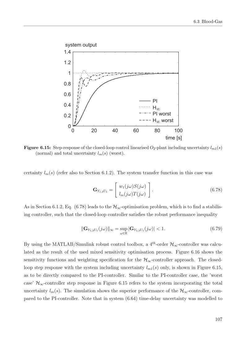
6.3 Blood-Gas
1.4
1.2
1
0.8
0.6
0.4
0.2
0
system output
0 20 40 60 80 100
time [s]
PI
H
PI worst
H worst
¥
¥
Figure 6.15: Step-response of the closed-loop control linearised O2-plant including uncertainty lm1(s)(normal) and total uncertainty lm(s) (worst).
certainty lm(s) (refer also to Section 6.1.2). The system transfer function in this case was
GY1,3U1 =
[w1(jω)S(jω)
lm(jω)T (jω)
]. (6.78)
As in Section 6.1.2, Eq. (6.78) leads to the H∞-optimisation problem, which is to find a stabilis-
ing controller, such that the closed-loop controller satisfies the robust performance inequality
‖GY1,3U1(jω)‖∞ = supω∈R
|GY1,3U1(jω)| < 1. (6.79)
By using the MATLAB/Simulink robust control toolbox, a 4th-order H∞-controller was calcu-
lated as the result of the used mixed sensitivity optimisation process. Figure 6.16 shows the
sensitivity functions and weighting specification for the H∞-controller approach. The closed-
loop step response with the system including uncertainty lm1(s) only, is shown in Figure 6.15,
as to be directly compared to the PI-controller. Similar to the PI-controller case, the ’worst
case’ H∞-controller step response in Figure 6.15 refers to the system incorporating the total
uncertainty lm(s). The simulation shows the superior performance of the H∞-controller, com-
pared to the PI-controller. Note that in system (6.64) time-delay uncertainty was modelled to
107

6 Control Design
20
10
0
-10
-20
-30
-40
magnitude [dB]
10-3 10-2 10-1 100 101
frequencyrads
S(j )w
T(j )w
w (j )1 w
l (j )m w
Figure 6.16: Sensitivity functions for robust stability and performance specification including thefrequency-dependent weightings for the H∞-controller.
the uncertain linearised TF (6.66) with the frequency weight approximation (6.71).
With the linearisation routine, as given in Section 6.3.2, the process is linearised for in-
put/output behaviour, but the process gain changes occur at different blood-flows qb. Since
the pO2-controller was tuned with high static gains in the lower operating area of qb, control
performance will degrade with higher flows, as there are lower system gains. This degradation
of control performance can be overcome with a gain-scheduled control, depending on arterial
flow qb. Therefore, the controller gain kp of the PI- and the H∞-controller were scheduled in
dependence of qb as
kp(qb) =
3kp0(qb − 1.5) ∀ qb ≥ 1.504 l/min
0.1kp0 ∀ qb < 1.504 l/min,(6.80)
where kp0 is the proportional controller gain. The saturation in Eq. (6.80) is to avoid negative
gains, when the blood-flow qb moves out of the operating range. However, during automatic
pO2-control blood-flows below the operating range limit of qb = 2 l/min lead to small controller
gains and the control response is slowed down.
Both, the PI- and the H∞-controller were finally discretised at the sampling time Ts,BGA = 6 s.
The controllers were implemented to the MATLAB/Simulink model for simulation evaluation.
108

6.3 Blood-Gas
6.3.4 pCO2-Controller Design
The control of the arterial carbon dioxide pressure is not so critical, compared with the pO2-
control. For the pCO2-process, the nonlinear static process gains differ far less than in the pO2
case and an input time-delay does not apply to the gas flow qg.
For pCO2-control, a PI-controller of the form (4.6) was tuned with the carbon dioxide plant.
The plant was approximated with a first order differential equation (time constant), output
time-delay and process gain to
GCO2(s) =kCO2
TCO2s + 1e−sTt,CO2 , (6.81)
with parameters to be found in Appendix B. The time constant TCO2 and the time-delay Tt,CO2
were adapted to the ’worst case’ process time-constant. For the process gain kCO2 , the static
gain value corresponding to a gas-flow of qg = 0.5 l/min and a blood-flow of qb = 2 l/min was
used.
Since the absolute value of the process gain |kCO2| decreases with blood-flow [46], the per-
formance of the controller will decrease with a rising blood-flow. This degradation of control
performance is similar to pO2-control and can be overcome with a gain-scheduling control. The
controller gain kCO2 of the PI-controller was scheduled in dependence of qb in the same way
as in (6.80). The operating region used for pO2-control applies also for pCO2-control, where
blood-flows below the operating range limit of qb = 2 l/min lead to a decelerated control re-
sponse. The CCO2-controller was finally discretised at a sampling time of Ts,BGA = 6 s and was
implemented to the MATLAB/Simulink model for simulation evaluation. The pCO2-controller
showed stability in simulation studies, tested over the whole operating range.
6.3.5 Blood-Gas Control Interconnection
pO2- and pCO2-control mechanisms were implemented and interconnected for simulation studies
as seen in Figure 6.17. To guarantee stability during the start of a simulation and in the real
plant, the control input variables uO2 = FiO2 and uCO2 = qg of both controllers were limited
(bounded away from zero, refer to Section 6.3.2). The discrete form of the CELC-PI- and the
CCO2-PI-controller were finally implemented in the discrete form
u(k) = fS [u(k − 1) + kp([kITs + 1]e(k)− e(k − 1))] , (6.82)
109

6 Control Design
with the proportional gain kp (kpO2for the pO2- and kpCO2
for the pCO2-controller), the integral
gain kI (kIO2for the pO2- and kICO2
for the pCO2-controller), the time at discrete sampling
time instances k, and a saturation function fS. This saturation function is of the same form
as (6.81). It has the lower and upper bounds a, b (aO2 , bO2 for the pO2- and aCO2 , bCO2 for the
pCO2-controller).
Y ( )•
x
-
-
CELC
y = x1 1
xss ss.e-s
^Td
ss
y = x ed 1-sTd
SimulatedPlant
v
CCO2
u = qCO g2
coxy
qb
-
y
(pCO )
2
2^
^
y
(pO )
1
2
LinearisationLoop
Discrete
Continuousr(pCO )
v2
2
r(pO )
v1
2 u = FiOO 22
Ts, BGA
y*Ts, BGA
Figure 6.17: Control strategy for pCO2- (upper part) and pO2-control (lower part). The estimatedstate space model ss for state linearisation is also implemented for the Smith-like predictor asss · e−sTd using the full process model with time-delay. ss denotes the state space model ofthe full time-delayed process (4.53), including time-delay and static gain (diffusion capacity)uncertainty. CELC is either the PI- or the H∞-external linear gain scheduled-controller.
110

7 Simulation and In-vitro Control Study
The different control systems developed in Chapter 6 were implemented in MATLAB/Simulink
for the simulation and in a real-time control environment (dSpace and XPC-Target) for the
in-vitro study. Closed-loop control performance was first studied in a simulation stage. In a
second stage, the controllers were tested in in-vitro experiments. Results of simulation and
in-vitro studies are shown in each section. Following the approach of Chapter 6, this chapter is
divided into haemodynamic and blood-gas control. Haemodynamic control is further divided
into arterial blood-flow and arterial pressure control. Each section shows stationary and pul-
satile control, for which simulation and experimental results are presented. Table 7.1 specifies
the order of appearance for the simulation and experimental results in this chapter.
Details on the experimental setup for the heart-lung machine, the haemodynamic vascular
system simulator and the blood-gas control setup are given in Appendix D.
During all simulation and in in-vitro experiments for haemodynamic control the vascular system
Table 7.1: Simulation and experimental results shown in this chapter.
Section Control Method Reference Setpoint Results
7.1 Blood-flow control Stationary Perfusion SimulationExperimental
Pulsatile Perfusion SimulationExperimental
7.2 Blood-pressure control Stationary Perfusion SimulationExperimental
7.3 Blood-pressure Pulsatile Perfusion Simulationboundary control Experimental
7.4 Blood-gas control Stationary Control Simulation(Step response) ExperimentalStationary Control Simulation(Disturbance) Experimental
111
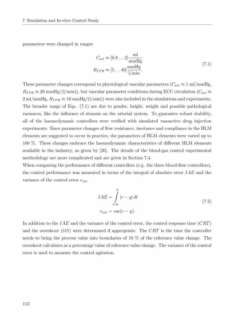
7 Simulation and In-vitro Control Study
parameters were changed in ranges
Cart ≈ [0.8 . . . 2]ml
mmHg
RTPR ≈ [5 . . . 40]mmHg
l/min.
(7.1)
These parameter changes correspond to physiological vascular parameters (Cart ≈ 1 ml/mmHg,
RTPR ≈ 20 mmHg/(l/min)), but vascular parameter conditions during ECC circulation (Cart ≈2 ml/mmHg, RTPR ≈ 10 mmHg/(l/min)) were also included in the simulations and experiments.
The broader range of Eqs. (7.1) are due to gender, height, weight and possible pathological
variances, like the influence of stenosis on the arterial system. To guarantee robust stability,
all of the haemodynamic controllers were verified with simulated vasoactive drug injection
experiments. Since parameter changes of flow resistance, inertance and compliance in the HLM
elements are suggested to occur in practice, the parameters of HLM elements were varied up to
100 %. These changes embrace the haemodynamic characteristics of different HLM elements
available in the industry, as given by [20]. The details of the blood-gas control experimental
methodology are more complicated and are given in Section 7.4.
When comparing the performance of different controllers (e.g. the three blood-flow controllers),
the control performance was measured in terms of the integral of absolute error IAE and the
variance of the control error evar
IAE =
T∫
t=0
|r − y| dt
evar = var(r − y).
(7.2)
In addition to the IAE and the variance of the control error, the control response time (CRT )
and the overshoot (OS) were determined if appropriate. The CRT is the time the controller
needs to bring the process value into boundaries of 10 % of the reference value change. The
overshoot calculates as a percentage value of reference value change. The variance of the control
error is used to measure the control agitation.
112

7.1 Arterial Blood-Flow Control
7.1 Arterial Blood-Flow Control
The three different controllers, developed in Section 6.1 were connected to the model of (4.24)
and simulated in stationary and pulsatile perfusion. The two sections below show also the
in-vitro results of the test series with the HLM and the hydrodynamic vascular system simu-
lator (MOCK). A detailed description of the hydrodynamic system simulator can be found in
Appendix D.1.
7.1.1 Stationary Perfusion
For stationary control, disturbances in the form of vasoactive substances and step-like setpoint
changes were applied over the whole flow operating range (qb = 0 . . . 6 l/min). Figure 7.1
shows a simulation of a typical system response to a control setpoint change of 2-3 l/min. The
system response of the PI-, the H∞- and the GPC- controller is given. The lumped vascular
system parameters that correspond to this simulation are Cart ≈ 2 ml/mmHg and RTPR ≈ 10
mmHg/(l/min). All three controllers were stable during the simulation test series and showed
good performance. The performance of the GPC-controller degraded in operating regions that
show a greater variance in system gain.
The results for the experimental study were similar to the results obtained in simulations. All
BFCs showed stability over the whole operating range and under varying vascular parameters.
Figure 7.2 shows the system response to a setpoint step of 2-3 l/min of an in-vitro experiment.
The parameters for the hydrodynamic system simulator that correspond to this experiment are
3.2
3
2.8
2.6
2.4
2.2
2
1.8
flow [l/min]
setpointsystem output GPCsysrem output PIsystem output Hinf
time [s]
0 0.5 1 1.5 2 2.5 3 3.5 4
Figure 7.1: Simulation step response of the three blood-flow controllers with modelled white noisesequence on the output.
113

7 Simulation and In-vitro Control Study
3.2
3
2.8
2.6
2.4
2.2
2
1.8
setpointsystem output GPCsysrem output PIsystem output Hinf
flow [l/min]
time [s]
0 0.5 1 1.5 2 2.5 3 3.5 4
Figure 7.2: Experimental step response of the three blood-flow controllers.
Cart ≈ 2 ml/mmHg and RTPR ≈ 10 mmHg/(l/min). The results of the experimental study were
similar to the results obtained in the simulation, although the control response in simulation
was a bit faster. The H∞-controller showed the best results, whereas the GPC-controller was
near instability in operating regions of a greater variance in system gain (which is mainly due
to the nonlinear static gain of the rotary blood pump and the aortic cannula). The control
response time (CRT ) during all simulations and experiments remained below CRT = 1 s with
all three controllers and below CRT = 0.5 s with the PI- and the H∞-controller. Table 7.2
summarises the results of a few exemplary BFC tests under in-vitro conditions. The IAE of the
H∞-controller is about half of the PI-controller. The GPC-controller gives the worst results,
which is because of the more ’sluggish’ control. As an indicator for haemolysis, the control
error variance of the H∞-controller is somewhat higher than that of the PI-controller.
Figure 7.3 shows an example for an experiment with stationary BFC and disturbance rejection
during time-varying system parameters. The blood-flow is kept constant at 3 l/min. At the
same time the TPR was changed by the clamping of the tube and pressure disturbance steps
Table 7.2: Performance of the three stationary blood-flow controllers at different operating pointsand under in-vitro conditions. MOCK parameters: TPR = 15 mmHg/(l/min), C = 1.5 ml/mmHg.
Performance index IAE [norm] ×103 var(ec) ×103
Steps to setpoint 1-2 l/min 2-3 l/min 3-4 l/min 1-2 l/min 2-3 l/min 3-4 l/min
GPC 142.9 305.6 193.2 31.2 72.7 52PI 74.6 63.9 57 35.3 28.6 29.2H∞ 24.5 30.56 28.6 38.2 32.1 29.2
114

7.1 Arterial Blood-Flow Control
22.5
33.5
4
flow[l/min]
050
100150200
pressure[mmHg]
010203040
TPR[mmHg/(l*min )]
-1
0 50 100 150 200 250 300 350 400 450 500 5501
1.5
2
2.5
time [s]
C[ml/mmHg]
setpoint
system output
8 10 12 14 16 18 20 22 241
1.2
1.4
1.6
1.8
2
2.2
C[ml/mmHg]
TPR [mmHg/(l*min )]-1
A
A
B
B
C
C
D
D
A
B
CD
Figure 7.3: PI-blood-flow control experiment with time-varying MOCK parameters and pressuredisturbances. The points A,B,C and D in the lower part of the figure refer to the time course ofpressure and flow values in the upper part of the figure.
were used to change the water level in the compliance chamber. Both TPR and compliance
changes were recorded with the MOCK control computer and are shown in the lower part of
Figure 7.3. This variation of vascular parameters is higher than in a real ECC. The high value
of the TPR for example leads to unphysiological high pressures. All controllers showed a very
115
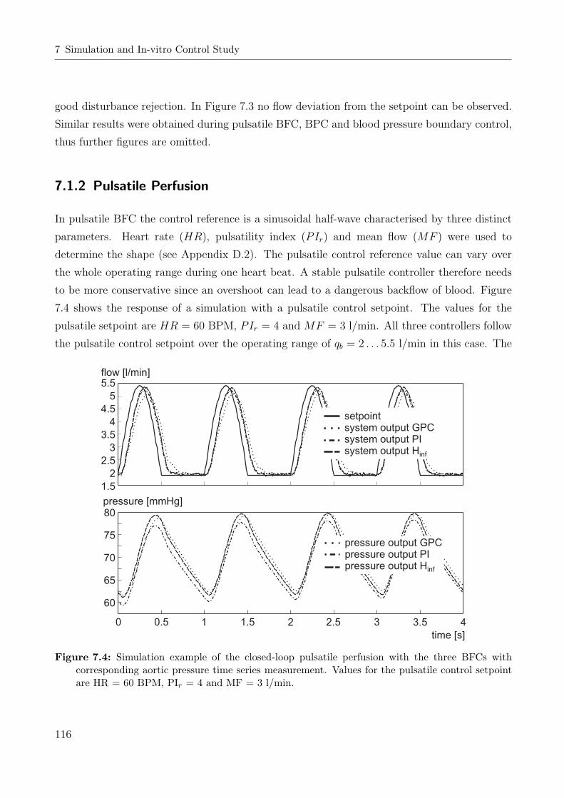
7 Simulation and In-vitro Control Study
good disturbance rejection. In Figure 7.3 no flow deviation from the setpoint can be observed.
Similar results were obtained during pulsatile BFC, BPC and blood pressure boundary control,
thus further figures are omitted.
7.1.2 Pulsatile Perfusion
In pulsatile BFC the control reference is a sinusoidal half-wave characterised by three distinct
parameters. Heart rate (HR), pulsatility index (PIr) and mean flow (MF ) were used to
determine the shape (see Appendix D.2). The pulsatile control reference value can vary over
the whole operating range during one heart beat. A stable pulsatile controller therefore needs
to be more conservative since an overshoot can lead to a dangerous backflow of blood. Figure
7.4 shows the response of a simulation with a pulsatile control setpoint. The values for the
pulsatile setpoint are HR = 60 BPM, PIr = 4 and MF = 3 l/min. All three controllers follow
the pulsatile control setpoint over the operating range of qb = 2 . . . 5.5 l/min in this case. The
0 0.5 1 1.5 2 2.5 3 4
time [s]
3.5
5.5
5
4.5
4
3.5
3
2.5
2
1.5
80
75
70
65
60
pressure [mmHg]
flow [l/min]
setpointsystem output GPCsystem output PIsystem output Hinf
pressure output GPCpressure output PIpressure output Hinf
Figure 7.4: Simulation example of the closed-loop pulsatile perfusion with the three BFCs withcorresponding aortic pressure time series measurement. Values for the pulsatile control setpointare HR = 60 BPM, PIr = 4 and MF = 3 l/min.
116

7.1 Arterial Blood-Flow Control
H∞-controller achieved the best results accompanied by the highest pressure variation in the
aortic arch. The lumped vascular system parameters that correspond to this simulation are
Cart ≈ 2 ml/mmHg and RTPR ≈ 20 mmHg/(l/min). Simulation test series were repeated with
simulated vasoactive substance injections and pressure disturbances and the controllers showed
stability and sufficient performance.
In experiments with the hydrodynamic system simulator, the pulsatile perfusion was validated.
Figure 7.5 shows an example of a pulsatile perfusion with the three BFC’s. The values for
the pulsatile setpoint are HR = 40 BPM, PIr = 4 and MF = 3 l/min. In the lower part
of Figure 7.5, the pressure variation measured in the aortic arch of the MOCK is given. The
MOCK parameters that correspond to this experiment are Cart ≈ 2 ml/mmHg and RTPR ≈ 20
mmHg/(l/min). In accordance with the measurements, the pressure variation generated by the
GPC-controller shows the worst results and is outmatched by the PI- and the H∞-controller.
The control response of the H∞-controller is faster than that of the PI-controller. Therefore
the H∞-controller shows slightly more pressure variation in the corresponding pressure curve.
0 0.5 1 1.5 2 2.5 3 4
time [s]
3.5
5.5
5
4.5
4
3.5
3
2.5
2
1.5
80
75
70
65
60
55
pressure [mmHg]
flow [l/min]
setpointsystem output GPCsystem output PIsystem output Hinf
pressure output GPCpressure output PIpressure output Hinf
Figure 7.5: Experimental example of the closed-loop pulsatile perfusion with the three BFCs withcorresponding aortic pressure measurement. Values for the pulsatile control setpoint are HR =40 BPM, PIr = 4 and MF = 3 l/min.
117

7 Simulation and In-vitro Control Study
The three BFCs were tested under different vascular conditions (7.1) and with various values
for the pulsatile setpoint. Stable control was achieved over these operating conditions, but the
control performance degraded with higher heart rates. The GPC-controller, in particular due
to the lower sampling time, cannot guarantee a pulsatile perfusion with higher HRs. In case of
a HR ≥ 60 BPM, the result of the GPC-controller is an almost stationary perfusion. PI- and
H∞-controller can provide pulsatile perfusion at higher HRs. Figure 7.6 depicts the result of
a MOCK measurement with the pulsatile values HR = 70 bpm, PIr = 4 and MF = 3 l/min.
The pressure course has a good variation, but the effect of turbulent flows on the pressure can
be seen in the sharp peaks in both curves.
In Table 7.3, control performance indices are listed for two pulsatile perfusion examples with
the three blood-flow controllers. The IAE and control error variance in the measurements at
a HR of 40 BPM show a great difference to that of a HR of 70 BPM. At 40 BPM the PI- and
the H∞-controller are superior to the GPC-controller. That is because they are able to follow
the pulsatile control setpoint. At a HR of 70 BPM a larger phase shift can be observed (see
0 0.5 1 1.5 2 2.5 3 4
time [s]
3.5
setpointsystem output GPCsystem output PIsystem output Hinf
pressure output GPCpressure output PIpressure output Hinf
6
4
2
0
90
80
70
60
50
flow [l/min]
pressure [mmHg]
Figure 7.6: Experimental example of the closed-loop pulsatile perfusion with the three BFCs withcorresponding aortic pressure measurement. Values for the pulsatile control setpoint sinusoidalhalf-wave are HR = 70 BPM, PIr = 4 and MF = 3 l/min.
118

7.2 Total Arterial Pressure Control
Figure 7.6), which leads to a large value in both performance indices. The IAE and the control
error variance are in that case no measure for the pulsatile performance of control.
Table 7.3: Performance of the three pulsatile blood-flow controllers at different operating pointsunder in-vitro conditions. Lumped MOCK parameters: TPR = 15 mmHg/(l/min), C = 1.5ml/mmHg.
Performance index IAE [norm] ×103 var(ec) ×103
HR, [BPM] 40 70 40 70
GPC 1020 1840 1680 4080PI 670 2240 840 8130H∞ 651 2470 887 9580
7.2 Total Arterial Pressure Control
The blood pressure PI-controller developed in Section 6.2.1 was connected to the model (4.24)
with the corrected line pressure as the system output. The corrected arterial pressure was then
low-pass filtered for noise reduction (fg = 15 Hz) and fed back to be compared to the control
setpoint. Figure 7.7 shows a simulated step response of the arterial blood pressure controller
in the typical operating range. The more ’sluggish’ control response of the pressure control
compared to the blood-flow control is due to the transfer function time constant, which is big-
ger than that of the arterial blood-flow output. In addition to that, the noise filter limits the
bandwidth of the control system to a further extent. The PI-controller was stable during all
simulations with different vascular and HLM parameters and during simulated vasoactive sub-
stance injections. The lumped vascular system parameters that correspond to this simulation
are Cart ≈ 1.5 ml/mmHg and RTPR ≈ 10 mmHg/(l/min) and correspond to the ECC case.
Figure 7.7 also shows the response of the arterial BPC to a control setpoint step of 20 to 50
mmHg. The vascular parameters of this experiment were set to values of Cart ≈ 2 ml/mmHg
and RTPR ≈ 10 mmHg/(l/min). The control response time is about 1 s with a small overshoot
of less than 10 %. The two control responses shown in Figure 7.7 differ mainly in the CRT ,
which is due to the difference in the compliance. The difference in the compliance originates
due to additional compliances in the 9th order vascular model. Similar results to Figure 7.7
were achieved over the whole operating range, where in regions of decreasing static system gain
119

7 Simulation and In-vitro Control Study
time [s]
pressure [mmHg]
pressure setpointsytem output simulationsystem output MOCK
0 0.5 1 1.5 2 2.5 3 3.5 4
55
45
35
25
15
Figure 7.7: Experimental example of the closed-loop stationary pressure control with the PI-BPC.Lumped MOCK parameters were TPR = 10 mmHg/(l/min), C = 2 ml/mmHg.
the overshoot is diminished but the control response time increases to about 1.5 s. Though
the control response is relatively fast and gives good results, the flow can take unphysiological
values during CPB. This can be caused by different means such as the rapid drop in TPR (see
discussion below). Figure 7.8 depicts a comparison of a simulation and an experimental result,
where the MOCK parameters are the same as the simulation parameters. The control system
in both cases is subject to a setpoint step of 30-50 mmHg. In addition to the arterial pressures
the corresponding aortic flow is given.
7.3 Arterial Pressure Boundary Control
The cascaded control structure of Section 6.2.2 was implemented in MATLAB/Simulink with
the model of (4.24). Similar to Section 7.1 the BFC (inner control loop) could be operated in
stationary and pulsatile perfusion. The pressure boundary control (PBC) is stable in stationary
control and except for the pressure correction based on the pressure boundary, the results are
congruent with Section 7.1. Therefore, the figures for stationary PBC will be omitted in this
section.
In pulsatile perfusion, for which a simulation example is shown in Figure 7.9, the corrected
(controlled) aortic pressure is given in the upper part of the figure with the corresponding
arterial line flow in the lower part. The three arterial flow curves are the reference value for
the flow, the flow reference value corrected by the PBC and the system output. The closed-
loop BFC operated at a HR = 60 BPM, a PIr = 4 and a MF = 3 l/min, when a pressure
120
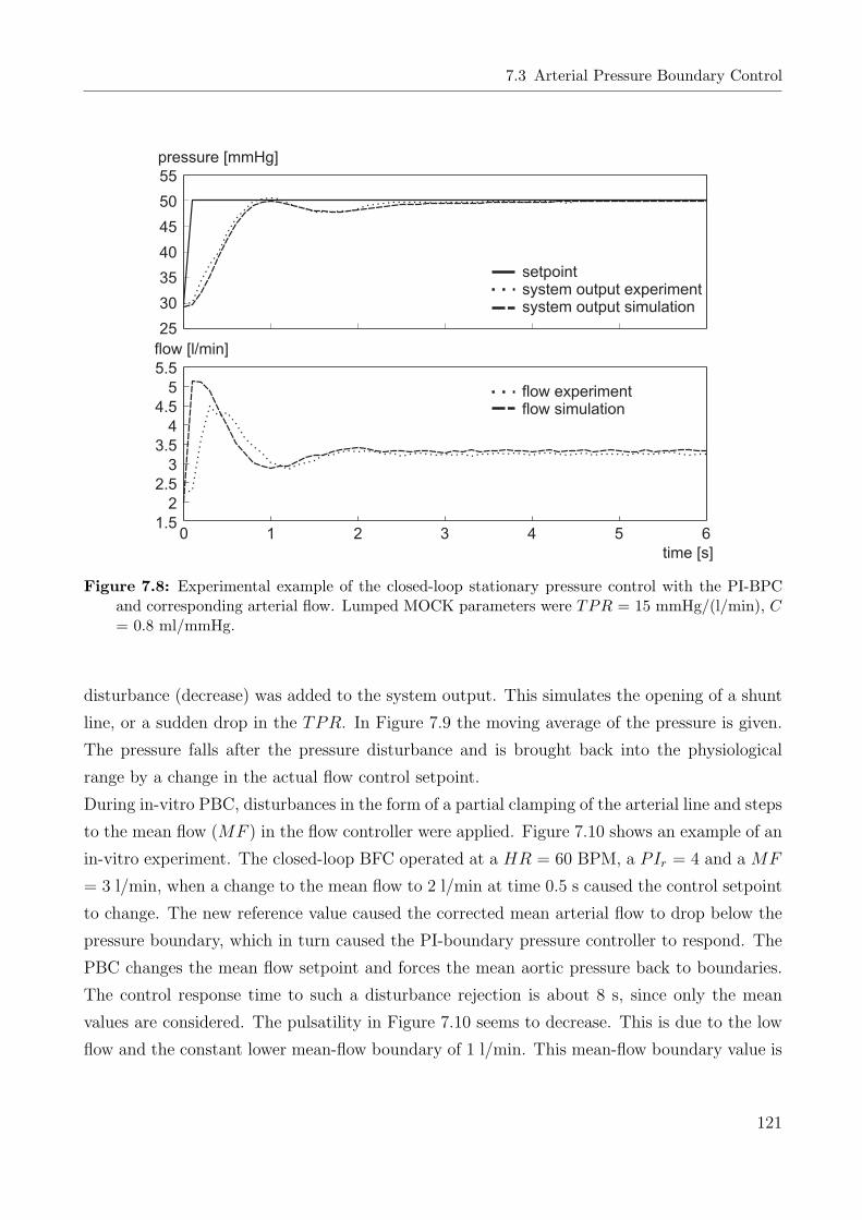
7.3 Arterial Pressure Boundary Control
pressure [mmHg]
flow [l/min]
0
time [s]
55
50
45
40
35
30
25
5.5
5
4.5
4
3.5
3
2.5
2
1.51 2 3 4 5 6
setpointsystem output experimentsystem output simulation
flow experimentflow simulation
Figure 7.8: Experimental example of the closed-loop stationary pressure control with the PI-BPCand corresponding arterial flow. Lumped MOCK parameters were TPR = 15 mmHg/(l/min), C= 0.8 ml/mmHg.
disturbance (decrease) was added to the system output. This simulates the opening of a shunt
line, or a sudden drop in the TPR. In Figure 7.9 the moving average of the pressure is given.
The pressure falls after the pressure disturbance and is brought back into the physiological
range by a change in the actual flow control setpoint.
During in-vitro PBC, disturbances in the form of a partial clamping of the arterial line and steps
to the mean flow (MF ) in the flow controller were applied. Figure 7.10 shows an example of an
in-vitro experiment. The closed-loop BFC operated at a HR = 60 BPM, a PIr = 4 and a MF
= 3 l/min, when a change to the mean flow to 2 l/min at time 0.5 s caused the control setpoint
to change. The new reference value caused the corrected mean arterial flow to drop below the
pressure boundary, which in turn caused the PI-boundary pressure controller to respond. The
PBC changes the mean flow setpoint and forces the mean aortic pressure back to boundaries.
The control response time to such a disturbance rejection is about 8 s, since only the mean
values are considered. The pulsatility in Figure 7.10 seems to decrease. This is due to the low
flow and the constant lower mean-flow boundary of 1 l/min. This mean-flow boundary value is
121
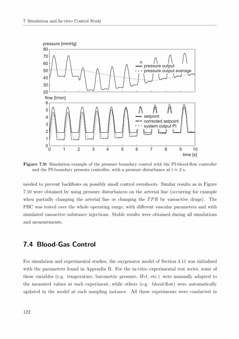
7 Simulation and In-vitro Control Study
0 1 2 3 4 5 6 7 8 9 10
time [s]
pressure [mmHg]
flow [l/min]
setpointcorrected setpointsystem output PI
pressure outputpressure output average
6
5
4
3
2
1
0
80
70
60
50
40
30
20
Figure 7.9: Simulation example of the pressure boundary control with the PI-blood-flow controllerand the PI-boundary pressure controller, with a pressure disturbance at t ≈ 2 s.
needed to prevent backflows on possibly small control overshoots. Similar results as in Figure
7.10 were obtained by using pressure disturbances on the arterial line (occurring for example
when partially clamping the arterial line or changing the TPR by vasoactive drugs). The
PBC was tested over the whole operating range, with different vascular parameters and with
simulated vasoactive substance injections. Stable results were obtained during all simulations
and measurements.
7.4 Blood-Gas Control
For simulation and experimental studies, the oxygenator model of Section 4.11 was initialised
with the parameters found in Appendix B. For the in-vitro experimental test series, some of
these variables (e.g. temperature, barometric pressure, Hct, etc.) were manually adapted to
the measured values at each experiment, while others (e.g. blood-flow) were automatically
updated in the model at each sampling instance. All these experiments were conducted in
122

7.4 Blood-Gas Control
time [s]
60
50
40
30
20
pressure [mmHg]
6
5
4
3
2
1
0
flow [l/min]
0 1 2 3 4 5 6 7 8 9 10
reference setpointcorrected reference setpointsystem output
Figure 7.10: Experimental example of the pressure boundary control with the PI blood-flow con-troller and the PI-pressure boundary controller. The mean flow setpoint changes at 0.5 s.
a strict predefined procedure, detailed in Appendix D.3. The controllers were tested over a
range of blood-flows (see below) and varying operating conditions such as temperature and
haematrocrit (Hct). Besides the changing blood-flow during a real CPB procedure mainly
temperature and Hct influence the static nonlinear process characteristics and have therefore
to be taken into account. However, the condition of the oxygenator (occlusion because of blood
platelet degradation) as a more severe influence on the nonlinear process characteristics was
not adapted in the state-predictor model. Experimental studies were conducted under varying
blood temperature and Hct conditions of
Tb ≈ [24 . . . 32], C Hct ≈ [21 . . . 36] %, (7.3)
which correspond to common values for most ECC procedures, given in literature [62, 68, 129].
In addition to the verification of stability of the controllers in all operating regions of interest,
three different types of tests were applied.
1. Disregarding the current state of the process, the controllers were switched-on. In sim-
123

7 Simulation and In-vitro Control Study
ulation the states at time zero were 0. During the in-vitro test series, the states of the
process were venous conditions or manually set-up pO2- or pCO2-values. The results of
controller switch-on as a special form of a step response will be shown in Section 7.4.1.
2. The responses to step-like setpoint changes were recorded in different operating regions.
3. As a direct disturbance to the BGA the extracorporeal blood-flow was changed over the
normal operating range 2 ≤ qb ≤ 5 l/min.
A total of 10 test series was conducted with primed porcine blood, where the different experi-
mental boundary conditions were set up. Furthermore, some of these test series were conducted
for up to eight hours of continuous blood circulation. Hence, a partial occlusion of the oxygena-
tor can be assumed in addition to the highly blood traumatising effects due to turbulent pump
flows. The high blood-flows (up to 6 l/min) and the long perfusion time caused the Hct value
of the primed blood to drop below 14 % at the end of some of the measurements. The results
from the simulation and in-vitro experimental study are shown in the following two sections.
Details on the experimental in-vitro setup can be found in Appendix D.3.
7.4.1 Stationary Blood-Gas Control (Step-Response)
The blood-gas partial pressures should be generally kept over a value of about 100 mmHg (about
97 % O2-saturation in normal, unstressed circulation conditions). On the other hand, the pO2
pressure of the venous system in the mean is about 40 mmHg (about 71 % O2-saturation
in normal conditions). The venous saturation value depends on blood-flow and on the O2-
consumption rate, which is about 120 ml/min O2 at 28C body temperature [29, 62] (about
240 ml/min O2 at 37C body temperature). Since different variables such as pH, temperature,
2,3-DPG and pCO2 can cause a right-shift to the oxygen saturation curve, a higher pO2 than
100 mmHg should be kept to maintain a sufficient oxygen supply. Too high pO2-values on the
other hand can lead to cerebral and tissue damage. A suggested value of 160 mmHg for arterial
oxygen partial pressure can be found in the literature, where arterial carbon dioxide partial
pressure should be kept at 40 mmHg. For most of the simulation and experimental results
the controllers were tested with the following values, considered as ’normal’ for ECC, shown in
Table 7.4. If not otherwise mentioned, these values are the conditions for the figures and tables
following below. ’On-switching’ of the controllers leads (like setpoint changes) to a transient
response.
124

7.4 Blood-Gas Control
Table 7.4: Values for BGA and control considered as ’normal’ during ECC.
Variable Value Variable Value
qb 4 l/min Pbaro 760 mmHgHct 21 % pO2,v 40 mmHgHb 6.96 g/dl pCO2,v 46 mmHgTb 28 C
On-Switch Simulation
In simulation the controllers were switched on with the initial model (zero states). In reality,
when switching on the controllers, the process is already in a certain state and the transient
response is assumed to vary strongly from that of simulation (see below). Figure 7.11 shows the
transient response of the PI- and the H∞-controller. The system response of the H∞-controller
has more overshoot but the faster CRT (about 50 sec faster). The transient response of the PI-
pCO2-controller in both simulations is the same. On-switching of the controllers was simulated
time [s]
250
200
150
100
50
0
4540353025201510
50
pO2 [mmHg]
pCO2 [mmHg]
0 20 40 60 80 100 120 140 160 180 200
pO setpointH processPi process
2
inf
pCO setpointpCO process (PI)
2
2
Figure 7.11: Simulation of blood-gas control switch-on.
125

7 Simulation and In-vitro Control Study
with different model conditions (see above) and at different flows. The results are similar to
those of Figure 7.11, with stability given in all simulations. Table 7.5 shows the performance
of the transient response after on-switching of the controllers. The simulation results shown in
Table 7.5 at a shunt value of 70 % refer to a reduction of the diffusion capacities in the process
model of the oxygenator to 70 %. The values of Table 7.5 confirm the simulation results of
Figure 7.11 with theH∞- being superior to the PI-controller. With the change in the oxygenator
diffusion capacities the higher gain of the H∞-controller leads also to a higher CRT in addition
to the higher overshoot. In the simulated occluded oxygenator case, the performance of the
PI-controller increases. This is a result of the uncertainties modelled to the nonlinear process.
On-Switch Experiment
In experimental in-vitro conditions, the effect of partial oxygenator occlusion could not be
determined exactly in terms of percentage loss of diffusion capacity. However, on-switching of
the controllers was conducted directly at the beginning of an experiment, and again after four
hours of continuous blood circulation. Figure 7.12 shows the experimental transient response
after on-switching of the controller at four hours of continuous circulation, which is suggested to
correspond to a shunt occlusion and a diffusion capacity reduction. The arterial pre-switching
conditions in that experiment were pO2,a ≈ 100 mmHg and pCO2,a ≈ 45 mmHg, whereas
responses of the gain-scheduled pCO2-controller in each of the two experiments were the same.
The final steady-state values of the FiO2-control input (lower part of Figure 7.12) differ by
about ≤ 1 %. This is due to a change in the process gains. Note that the experiments shown
in Figure 7.12 could not be executed at the same time and so the time offset between those two
experiments already caused a diffusion capacity loss at the PI-control experiment. The CRT
of the H∞-controller is about 40 seconds faster in the partially occluded system, whereas the
total CRT of both controllers is a lot more sluggish in the in-vitro experiment, see Table 7.6.
Table 7.5: Performance of the PI- and the H∞-controller in simulation after on-switch.
Simulation IAE [norm] OS [%] CRT [s] var(ec)
Normal PI 1114 5.62 102 2625.5Normal H∞ 942 23.75 48 2833.3Shunt (70 %) PI 952 19.37 66 2680.6Shunt (70 %) H∞ 1013 26.25 84 2893.8
126

7.4 Blood-Gas Control
180
160
140
120
100
pO [mmHg]2 pCO [mmHg]2
FiO [%]2
36
34
32
30
28
26
24
20
18
q [l/min]Gas
54.5
43.5
32.5
21.5
10.5
0 0100 100200 200300 300400 400500 500
time [s] time [s]
50
45
40
35
30
pO setpointH processPI process
2
inf
pCO setpointpCO process
2
2
H control inputPI control input
inf
Figure 7.12: Experiment of a blood-gas control switch-on with control input actuating variables inthe lower part.
As already mentioned above, this is caused by the exited process differing from the states of
the linearisation and prediction model. The H∞ CRT at the start of the experiment is only 20
seconds faster than the CRT of the PI-controller. This agrees with the simulation results, where
the PI-controller was faster with the occluded system. In in-vitro experimental conditions,
however, the H∞-controller is faster in both cases. Regarding CRT and an overshoot of less
than 10 %, the results for the non-occluded oxygenator control switch-on are better than those
of the partially occluded oxygenator. However, both transient switch-on responses (and all other
transient responses with different arterial pre-control conditions) are far from instability. Table
7.6 shows the experimental performance of the two controllers at different experimentation
times. Entries (start) in Table 7.6 refer to measurements that were conducted directly after
the start of the experiment or after four hours of continuous perfusion (4 hours). Comparing
the experimental results of Table 7.6 to simulation results of Table 7.5 one can see that in the
in-vitro experiment the IAE is approximately doubled, but the variance of control errors is a lot
lower. This is due to the more ’sluggish’ response in in-vitro switch-on (note that the variance
127

7 Simulation and In-vitro Control Study
var(ec) was chosen as a measure for agitation during control). The results of the gain-scheduled
pCO2-controller in simulation and in in-vitro conditions are far less critical than those of the
pO2-controllers. Figure 7.11 and 7.12 also show the transient pCO2-process value response
after on-switching of the pCO2-controller. The pCO2-controller switch-on without initial state
adaption leads to a drop in total gas-flow directly after the start of the experiment. Note that
this in-process on-switching without adaption to the process states was conducted as a sort of
’worst case’ on-switching. Furthermore, no significant difference in control performance indices
were found in simulation and in-vitro experiments at different oxygenator shunt fraction values.
This emphasises the the result from the modelling section, that the pCO2-process nonlinearities,
varying time constant and time-delay are less critical for control.
Table 7.6: Performance of the PI- and the H∞-controller in the in-vitro experiment after on-switch.
Experiment IAE [norm] OS [%] CRT [s] var(ec)
PI (start) 1968.3 6.87 210 741.24H∞ (start) 1945.5 4.53 192 695.4PI (4 hours) 1977.7 0 240 492.83H∞ (4 hours) 1959.3 0 204 701.13
Step Response Simulation
During experiments, control reference changes in the form of steps were applied to the steady
state PI- and H∞-controlled system in the normal range of operating points. An example of a
simulation step response with an oxygenator shunt fraction of 100 % (full diffusion capacity) can
be seen in Figure 7.13. In the steady-state controlled condition, the reference value was changed
from 120 to 160 mmHg, showing PI- and H∞-controller system responses. The robustly tuned
H∞-controller has less overshoot (22.5 % in contrast to 45 %), whereas the control response
time of the PI-controller is about 20 seconds faster. The FiO2 control-input of both controllers
can be seen in the lower part of Figure 7.13. Steps were applied in other operating areas over
the whole operating range (pO2 = [100...250] mmHg) and similar results were obtained. The
simulations of reference value step changes were repeated with other blood-flow values (change
in linearised system gain) and the effect of the gain-scheduling was examined. However, results
are similar to those shown in Figure 7.13.
To simulate the result of a partially occluded oxygenator, the diffusion capacities in the model
128

7.4 Blood-Gas Control
0 10 20 30 40 50 60 70 80 90
time [s]
180
170
160
159
140
130
120
40
35
30
25
20
pO setpointH processPI process
2
inf
H control inputPI control input
inf
pO [mmHg]2
FiO [%]2
Figure 7.13: Simulation of a blood-gas control step-response from 120-160 mmHg.
were changed to 70 % (see above) and simulation was repeated. Figure 7.14 shows the result of
a step response with the occluded oxygenator. In this case, the H∞-controller has a more ’slug-
gish’ response compared to that of the PI-controller which reacts faster with more overshoot.
Control simulations with 70 % oxygenator diffusion capacities were repeated over the whole
process operating range and at different flows (see above) and stability and performance were
ascertained. Table 7.7 summarises the results of control performance indices for the two step
response simulations. Values of IAE and control error variance do not differ much. Serious
differences can be found in the OS and CRT . As already seen in the transient response at
Table 7.7: Step-response performance of the PI- and the H∞-controller in simulation.
Simulation IAE [norm] OS [%] CRT [s] var(ec)
Normal PI 177 45 36 153.75Normal H∞ 171 22.5 60 141.98Shunt (70 %) PI 172 35 42 148.8Shunt (70 %) H∞ 188 22.5 60 148.16
129
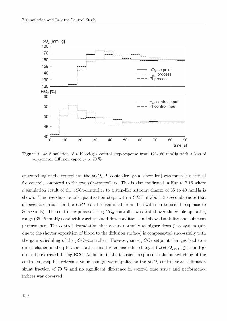
7 Simulation and In-vitro Control Study
0 10 20 30 40 50 60 70 80 90
180
170
160
159
140
130
120
60
55
50
45
40
pO setpointH processPI process
2
inf
H control inputPI control input
inf
time [s]
pO [mmHg]2
FiO [%]2
Figure 7.14: Simulation of a blood-gas control step-response from 120-160 mmHg with a loss ofoxygenator diffusion capacity to 70 %.
on-switching of the controllers, the pCO2-PI-controller (gain-scheduled) was much less critical
for control, compared to the two pO2-controllers. This is also confirmed in Figure 7.15 where
a simulation result of the pCO2-controller to a step-like setpoint change of 35 to 40 mmHg is
shown. The overshoot is one quantisation step, with a CRT of about 30 seconds (note that
an accurate result for the CRT can be examined from the switch-on transient response to
30 seconds). The control response of the pCO2-controller was tested over the whole operating
range (35-45 mmHg) and with varying blood-flow conditions and showed stability and sufficient
performance. The control degradation that occurs normally at higher flows (less system gain
due to the shorter exposition of blood to the diffusion surface) is compensated successfully with
the gain scheduling of the pCO2-controller. However, since pCO2 setpoint changes lead to a
direct change in the pH-value, rather small reference value changes (|∆pCO2,ref | ≤ 5 mmHg)
are to be expected during ECC. As before in the transient response to the on-switching of the
controller, step-like reference value changes were applied to the pCO2-controller at a diffusion
shunt fraction of 70 % and no significant difference in control time series and performance
indices was observed.
130

7.4 Blood-Gas Control
pCO setpoint2
pCO system output2
41
40
39
38
37
36
35
qg [l/min]
2.5
2
1.5
1
0.50 10 20 30 40 50 60 70 80 90
time [s]
q control inputg
pCO [mmHg]2
Figure 7.15: Simulation step response of the pCO2-PI-controller to a step-like setpoint change of35-40 mmHg.
Step Response Experiment
The same reference value changes that were applied to the two pO2-controllers in simulation
were now applied in in-vitro experimental conditions. For this purpose, step-like reference
value changes around the operating point of pO2 = 160 mmHg were applied to the PI- and
H∞-controllers. Figure 7.16 shows an example of a step-like reference value change of 120 to
160 mmHg of both controllers after four hours of continuous circulation. The H∞-controller
has more overshoot, but the faster CRT . Table 7.8 lists the results of a reference value change
of pO2,ref = 120-160 mmHg directly after the start of an experiment and of one after four
hours. In contrast to the simulation study, the OS of the H∞-controller is higher during the
experiment. The time series at the beginning of the experiment is similar to that after four
hours and is omitted. The performance of the H∞-controller in this experiment was inferior to
the PI-controller, with more overshoot and a higher CRT . Also note that the CRT in Table
7.8 is similar to that of the simulation results in Table 7.7. The OS in the experimental study is
even less. Furthermore, the values of IAE and the variance of the control error are only slightly
131

7 Simulation and In-vitro Control Study
pO setpointH processPI process
2
inf
H control inputPI control input
inf
time [s]
160
150
140
130
120
pO [mmHg]2
36
34
32
30
28
26
FiO [%]2
0 20 40 60 80 100 120 140 160 180
Figure 7.16: Experiment of a blood-gas control step-response from 120-160 mmHg after four hoursof continuous circulation.
Table 7.8: Step-response performance of the PI- and the H∞-pO2-controller in the in-vitro experi-ment.
Experiment IAE [norm] OS [%] CRT [s] var(ec)
PI (start) 217.55 5 42 219.97H∞ (start) 222.02 15 66 230.75PI (4 hours) 263.62 5 60 200.6H∞ (4 hours) 216.45 7.5 54 231.33
worse during the in-vitro experiment. As in the simulation study before, the pO2-controllers
were tested in a range of operating conditions (7.3), pO2 reference values and with varying flow.
Long-term measurements were conducted for up to eight hours of continuous circulation, with
high flow rates and partially occluded oxygenators. Sufficient performance was ascertained dur-
ing all experiments, where the performance did not seem to suffer from oxygenation diffusion
capacity loss. The CRT and the OS in other operating conditions/ranges were similar to those
of Table 7.8 and underlined the good performance of the controllers in in-vitro experiments.
For the experimental test of the gain-scheduled pCO2-controller, reference values of pCO2 =
132

7.4 Blood-Gas Control
35-45 mmHg were chosen (like in simulation before). Figure 7.17 shows an experimental result
of a step-response with a reference value change of 35 to 40 mmHg. The reference value was
changed in the steady-state control condition, with a gas-flow of about 5 l/min at the beginning.
The response of in-vitro pCO2-control is more ’sluggish’, with an approximately doubled CRT .
However, the CRT is hard to compare since the control OS of one quantisation step is already
20 %. Like the pO2-controllers, the pCO2-controller was tested with long-term measurements
of up to eight hours. Performance and stability were ascertained during all experimental mea-
surements under different operating conditions (see pO2-control above).
In addition to the simulation experiments mentioned above, pCO2-control was tested on sta-
bility within other temperatures and Hct values, following Equation (7.3). In the case of a
temperature shift, the control degraded compared to higher temperatures, but remained stable
with sufficient performance even up to high temperature values of 32 C. The results of these
studies are similar to the results presented above and are therefore omitted.
pCO setpoint2
pCO system output2
time [s]
q control inputg
42
41
40
39
38
37
36
35
pCO [mmHg]2
5
4.5
4
3.5
3
2.5
2
q [l/min]g
0 50 100 150 200 250 300 350
Figure 7.17: Experimental step response of the pCO2-PI-controller to a step-like setpoint change of35 to 40 mmHg.
133

7 Simulation and In-vitro Control Study
7.4.2 Stationary Blood-Gas Control (Disturbance Rejection)
By choosing the correct values for pO2 and pCO2, not only a sufficient oxygen supply but also
the correct pH-value are determined during CPB. The oxygen supply is also determined by
the blood-flow (which is due to the haemodynamical requirements and which should be auto-
matically controlled, Section 7.1). Even in closed-loop controlled condition, the mean arterial
blood-flow control will vary over the course of an CPB procedure. Right after onset of CPB,
the blood-flow is continually increased, when the heart is slowly brought to a resting condition.
The general guideline for the blood-flow of 2.4 l/min/m2 body surface is not met at the begin-
ning of a CPB. Furthermore, the blood-flow will be decreased in the weaning phase at the end
of CPB. In the onset and in the weaning stage, the HLM is driven in partial bypass condition
according to the conditions of the heart. During ECC, unwanted changes in flow may also not
be excluded, since perfusion technicians must be able to correspond to the patient’s current sit-
uations such as blood volume loss, leakage, adequate pressure maintenance or O2-consumption
rate change. Regarding this, a changing blood-flow can be seen as a direct disturbance to the
process states, which in turn carries forward to the system output, delayed only by blood-flow
dependent time-delay and BGA time constant. The pO2- and pCO2-controllers have to be
stable and respond adequately to blood-flow disturbances. This means that by changing the
blood-flow the partial oxygen pressure must not fall below 97 % oxygen saturation (≈ 100
mmHg) to guarantee a continuous oxygen supply. On the other hand, the pO2 value should
not stay at higher pressures (≥ 250 mmHg) to avoid cerebral, nervous and tissue damage. The
carbon dioxide partial pressure should be maintained at any time in the range of 35-45 mmHg
(better 37-43 mmHg) to guarantee an appropriate pH-value of the blood.
The blood-gas control experimental disturbance test series follow the same procedure as de-
scribed in Section 7.4.1. As normal conditions during ECC, values of Table 7.4 were adjusted to
simulate a cardiopulmonary bypass procedure in simulation and in in-vitro conditions. In ad-
dition to the changing blood-flow, controllers were tested in other operating conditions given in
Equation (7.3). The reference values for the disturbance blood-gas control test series are pO2,ref
= 160 mmHg and pCO2,ref = 40 mmHg (see Section 7.4.1). The blood-flow disturbance, which
was used for testing the controllers, was a stair function with step-like changes of 1 l/min in
the ranges qb = [2 . . . 5] l/min. Note that these abrupt flow changes are not likely to occur in
ECC, since such a flow change could cause severe tissue or vascular damage. These blood-flow
changes as accomplished in this work are therefore more conservative in control terms.
134

7.4 Blood-Gas Control
The blood-flow disturbance has an influence on both, pO2 and pCO2. Figure 7.18 shows the
result of a simulation with the PI-controller at 100 % oxygenator diffusion capacity. The tran-
sient response of the pO2-controller, which seems to be underdamped, is due to process coupling.
The simultaneous pCO2-controller intervention in gas-flow, used to correct the pCO2-value, also
influences the pO2-process. From Figure 7.18 can also be seen, that the pO2-value does not
exceed 200 mmHg nor does it fall below 140 mmHg. The flow disturbances for pCO2-control
are not by far as serious as in pO2-control. The pCO2-process value remains within ± 2 mmHg
of the reference value. The simulation was repeated with the H∞-controller and shows a similar
behaviour with the pO2-process value remaining within 140-200 mmHg. Table 7.9 shows the
control performance of the PI- and H∞-controller in simulation. During disturbance rejection,
larger control deviations occurred at lower flows. This is because of the larger time-delays that
are caused by the low blood-flow and the low gas-flow. Note that the pO2-process has input
and output time-delay and the control deviation at lower blood-flows is more severe.
The percentage overshoot values in this section are the maximum disturbance overshoot values
0 200 400 600 800 1000 1200 1400
time [s]
qb [l/min]
arterial line flow
pCO setpoint2
pCO system output2
pO setpoint2
pO system output2
200
150
100
50
0
40
30
20
10
0
5
4
3
2
1
pO [mmHg]2
pCO [mmHg]2
Figure 7.18: Response of the PI-pO2- and PI-pCO2-controllers to a blood-flow disturbance in simu-lation with oxygenator diffusion capacity of 100 %.
135

7 Simulation and In-vitro Control Study
Table 7.9: Disturbance rejection performance of the PI- and the H∞-controller in simulation.
Simulation IAE [norm] OS [%] var(ec)
Normal PI 1900 46.87 364.15Normal H∞ 1659 31.87 223.11Shunt (70 %) PI 901 21.25 73.15Shunt (70 %) PI H∞ 998 21.87 82.94
referring to pO2,ref = 160 mmHg. Therefore, a disturbance of for example 21.25 % would mean
an overshoot (undershoot) of 36 mmHg. The critical value for an overshoot in the experiments
is 62.5 %, which could mean a drop to pO2,a = 100 mmHg. In addition to the normal control
simulation, the performance values of a reduced oxygenator diffusion capacity of 70 % are given.
Figure 7.19 shows the result of a simulation with the H∞-controller at 70 % oxygenator diffu-
sion capacity. Note that this result is similar to that of Figure 7.18. Simulation disturbance
rejection series were repeated at different temperatures and Hct values (7.3), where similar
0
50
100
150
200
250
0
10
20
30
40
0 200 400 600 800 1000 1200 14001
2
3
4
5
time [s]
qb [l/min]
arterial line flow
pCO setpoint2
pCO system output2
pO setpoint2
pO system output2
pO [mmHg]2
pCO [mmHg]2
Figure 7.19: Response of the H∞-pO2- and PI-pCO2-controllers to a blood-flow disturbance in sim-ulation with oxygenator diffusion capacity of 70 %.
136

7.4 Blood-Gas Control
results to the performance of Table 7.9 were observed. During all simulations, the PI- and the
H∞-controller were stable and the OS did not exceed the critical value of 62.5 %.
Figure 7.20 depicts the result of an in-vitro experiment with the H∞-pO2-controller and PI-
pCO2-controller at a Hct value of 28 %. This measurement was conducted shortly after the
beginning of the experiment. The OS of the pO2-controller remains below the critical value
of 62.5 %, but the control response is a bit longer (as also the total time range of the experi-
ment is 1800 s in contrast to 1400 s in the simulation). The performance values IAE, OS and
variance of control error were calculated for four sample experiments directly at the onset of
simulation and after 4.5-5 hours at a temperature of 24C and 32C. Table 7.10 lists the results
for these sample experiments. Compared to the simulation of disturbance rejection, the IAE
almost doubles, but does not increase significantly with a partially occluded oxygenator. The
overshoot in pO2,a of the sample experiments, but also of all others in the whole experimental
in-vitro test series, is OS ≤ 25 %, which is a much better result than in simulation.
The time series of the experiments conducted at different temperatures is similar to that of
time [s]
pO setpointpO process
2
2
pCO setpointpCO process
2
2
200
150
100
50
0
50
40
30
20
10
0
6
5
4
3
2
1
qb [l/min]
pO [mmHg]2
pCO [mmHg]2
0 200 400 600 800 1000 1200 1400 1600 1800 2000
Figure 7.20: Response of the H∞-pO2- and PI-pCO2-controllers to a blood-flow disturbance in anexperiment with a Hct-value of 28 % after the beginning of circulation.
137
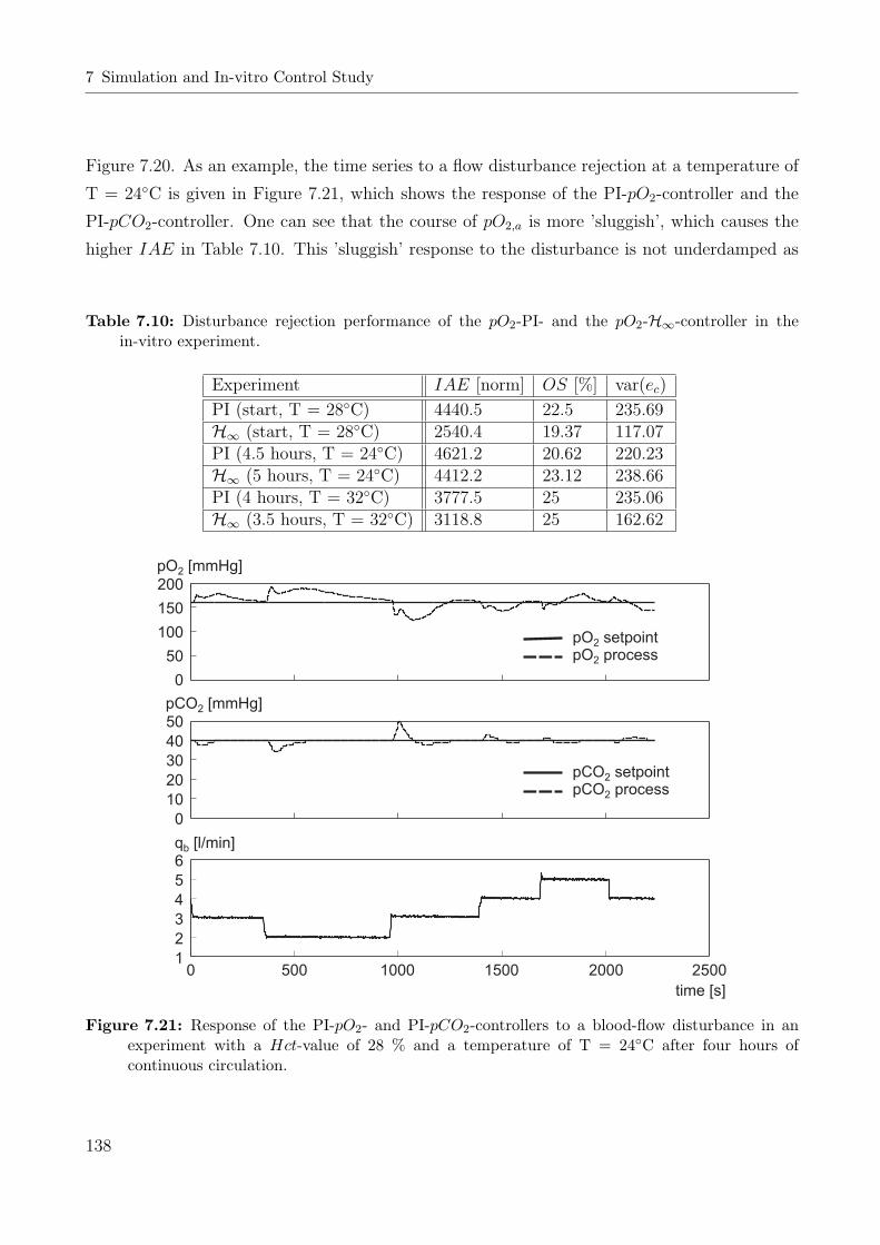
7 Simulation and In-vitro Control Study
Figure 7.20. As an example, the time series to a flow disturbance rejection at a temperature of
T = 24C is given in Figure 7.21, which shows the response of the PI-pO2-controller and the
PI-pCO2-controller. One can see that the course of pO2,a is more ’sluggish’, which causes the
higher IAE in Table 7.10. This ’sluggish’ response to the disturbance is not underdamped as
Table 7.10: Disturbance rejection performance of the pO2-PI- and the pO2-H∞-controller in thein-vitro experiment.
Experiment IAE [norm] OS [%] var(ec)
PI (start, T = 28C) 4440.5 22.5 235.69H∞ (start, T = 28C) 2540.4 19.37 117.07PI (4.5 hours, T = 24C) 4621.2 20.62 220.23H∞ (5 hours, T = 24C) 4412.2 23.12 238.66PI (4 hours, T = 32C) 3777.5 25 235.06H∞ (3.5 hours, T = 32C) 3118.8 25 162.62
pO setpointpO process
2
2
pCO setpointpCO process
2
2
200
150
100
50
0
50
40
30
20
10
0
6
5
4
3
2
1
qb [l/min]
pO [mmHg]2
pCO [mmHg]2
time [s]
0 500 1000 1500 2000 2500
Figure 7.21: Response of the PI-pO2- and PI-pCO2-controllers to a blood-flow disturbance in anexperiment with a Hct-value of 28 % and a temperature of T = 24C after four hours ofcontinuous circulation.
138
7.4 Blood-Gas Control
it seems, but due to the change in gas-flow, as a result of the PI-pCO2-disturbance rejection.
This leads, as in simulation, to a change in the pO2,a-process value and accumulates in addition
to the disturbance of the blood-flow. The result is even more severe than in simulation, since
a change in blood-flow changes the pCO2,v-value after the de-oxygenators (note that in simu-
lation the venous pCO2 pressure conditions were assumed to be constant). This effect is due
to the in-vitro-dependent O2-removal technique (see Appendix D.3.2) that changes the pCO2,v
much more strongly than in a real CPB. As a reaction to that, the pCO2-controller changes
the total gas-flow to the oxygenator. This in turn can be seen as a control disturbance on the
FiO2-input, as it is directly coupled to the gas-inflow (6.29).
The gain-scheduled PI-pCO2-control in the flow disturbance rejection experiments is far from
instability, but the OS induced by the blood-flow changes can be as high as 25 %. Note that this
must be distinguished from the results in the simulation studies, where the OS never exceeded
2 mmHg (5 %). In fact, these high OS values are caused by the deoxygenation technique
to simulate the human body (see Appendix D.3.2). The high diffusion capacity for carbon
dioxide DCO2,m and lower binding affinity lead to these large changes in the venous carbon
dioxide partial pressure condition, to which the pCO2-control has to respond. Hence, the PI-
pCO2-control has a slightly longer CRT , but works in terms of stability and performance as
predicted in simulation. Table 7.11 concludes with the performance values for simulation and
experimental in-vitro disturbance rejection test results. Note that the values of the in-vitro
experiments in Table 7.11 are inferior compared to simulations due to the reasons mentioned
above, but would be sufficient for ECC. Since the venous pCO2 is not subject to such fluctuation
on a blood-flow change, the pCO2-control strategy can be assumed to function even under worst
conditions.
To give an example of how control performs without coupling and deoxygenation technique dis-
Table 7.11: Disturbance rejection performance of the PI-pCO2-controller in simulation and in-vitroexperiment (EXP: Experiment, SIM: Simulation).
Test IAE [norm] OS [%] var(ec)
PI-pCO2 (normal) SIM 33 5.26 0.21PI-pCO2 (start) EXP 247.21 22.5 2.29PI-pCO2 (Sht 70 %) SIM 28 5.26 0.17PI-pCO2 (4.5 hours, T = 24C) EXP 299.41 25 2.72
139

7 Simulation and In-vitro Control Study
turbances, the pCO2-controller was deactivated and the performance of the pO2-controller was
tested alone. Figure 7.22 shows the result of a H∞-pO2-control in-vitro experiment. The perfor-
mance values of this experiment are IAE = 980.53, OS = 31.25 % and var(ec) = 150.23 and are
similar to the performance obtained in simulation. Since the venous conditions are not expected
to change much on a blood-flow change, a result similar to Figure 7.22 is expected in in-vivo
application with a real patient, with process coupling similar to the simulation examples. Even
if slight to little changes to venous conditions occur the control is stable and shows sufficient
performance (see examples with changing venous conditions above). A detailed description of
the de-oxygenation conditions and consequences can be found in Appendix D.3.2.
In Figure 7.22, it can be clearly seen, that the OS at lower blood-flows is higher than in other
blood-flow operating regions. This prolonged disturbance rejection is due to the higher time-
delay at lower blood-flows. In addition, the model-process mismatch, that derives from the
gas-valve error offset at lower gas-flows contributes to this effect.
250
200
150
100
50
0
pO [mmHg]2
5.5
5
4.5
4
3.5
3
2.5
2
1.5
qb [l/min]
time [s]
0 100 200 300 400 500 600 700 800 900
pO setpointpO process
2
2
Figure 7.22: Response of the H∞-pO2-controller to a blood-flow disturbance in an experiment afterfour hours of continuous circulation.
140

8 Conclusion and Discussion
The goal of this work was to develop automatic control strategies and algorithms for the con-
trol of cardiopulmonary heart-lung support. Although modern integrated heart-lung machines
comprised of several safety systems are available on the market, none with a feedback control
strategy exist up to now and important vital variables are still adjusted manually during the
surgical procedure. The main reason for this is the safety requirement. A closed-loop controller
may become unstable, which could cause damage to the patient. A closed-loop control algo-
rithm has therefore to satisfy robust stability in addition to the desired performance. Robust
stability must be guaranteed in a complex biological system coupled to an artificial organ, the
HLM. Difficulties for control are inherent in the system and comprise nonlinearities, parameter
uncertainties for different patients and pathological vascular variances, changing transport time-
delays and time-varying parameters induced by various drugs or physiological body’s agents.
Although, all these difficulties exist in the HLM and the human body, and some of these mech-
anisms are not well known up to the present, an automatic control is suggested to increase
the patient’s safety on the one hand and remove workload from the perfusionist technician on
the other hand. The well-known advantages of an automatic control, such as fast responses
to control reference changes and good disturbance rejection are expected to optimise the car-
diopulmonary bypass routine, thereby minimising the risk of tissue damage or inflammatory
response.
In addition to the difficulties that arise with the system that is to be controlled the right control
strategy has to be chosen. The question that arises in this context are mainly ’what’ should
be controlled and ’how’ concerning control inputs, reference variables and reference values. For
this reason, the physiological and technical background knowledge was presented (Chapter 2
and 3) and the literature on CPB control was critically examined. Among the most impor-
tant vital variables during CPB are certainly the haemodynamics and the blood-gas exchange,
bearing in mind that the HLM takes over the work of heart and lung (transport of blood and
oxygenation/carbon dioxide removal). Other control of vital variables, such as blood and body
141

8 Conclusion and Discussion
temperature or pH-value in the blood were not considered here. Blood and body temperature
are easily controlled by thermostats and in the case of pH-value anaesthetists prefer the manual
application of drugs. The haemodynamics (blood pressure and flow) and the blood-gas exchange
(oxygen and carbon dioxide partial pressures) were considered to be of main importance and
this work concentrated on the control of these vital variables. For control, a haemodynamic
and a blood-gas model were developed (Chapter 4), validated (Chapter 5) and controllers were
designed, based on these models (Chapter 6). The controllers were then validated in simulations
and in special in-vitro experiments (Chapter 7). In the in-vitro experiments, the physiological
human system was reproduced in parts by simulation circuits that simulate the physiological
behaviour of those systems. This is necessary before the application in in-vivo animal or human
test series.
The evident control actuator for haemodynamic control is the blood pump (artificial heart).
Based on the blood pump as the control actuator, three different control strategies were de-
veloped and compared to each other for performance [85]. A feedback control is proposed and
introduced for arterial flow, arterial pressure and combined arterial flow/pressure. In contrast
to other authors [18, 115, 123], in this work only arterial pressure and flow were controlled. In
a HLM system with a buffered venous bag the control of venous conditions plays a secondary
role. Furthermore, the use of vasoactive agents (vasoconstrictive or vasodilative) as an addi-
tional control actuator for arterial conditions, as for example used by [54, 61, 142] were avoided.
Vasoactive agents if applied over a longer time show severe adverse effects and are preferably
applied by anaesthetists manually.
For haemodynamic control, the system was divided in a technical and a physiological subsystem.
The technical subsystem, which comprised the haemodynamics of the HLM’s components, was
implemented in MATLAB/Simulink and was validated in experiments. Particular attention was
laid to the modelling of a rotary blood pump with diagonally streamed impeller. Experimental
results show a good agreement in static and frequency domain measurements. The physiologi-
cal system comprised the vascular system described by the linearised Navier-Stokes equations.
Two models varying in complexity were implemented in MATLAB/Simulink. These two mod-
els were then compared in the frequency range to real vascular frequency responses taken from
literature. As a result, the low order model, that can adequately describe the patient’s vessel
dynamics, was preferred to the high order model. This low order model was then extended with
equations for vasoactive drug distribution. In a next step, technical and physiological models
were implemented and interconnected in MATLAB/Simulink. For the development of control,
142

the model was finally linearised in its ’worst case’.
Based on this linearised model, three controllers were developed and tuned for arterial blood-
flow control. A PI- and a H∞-controller were tuned with the ’worst case’ linearised model,
whereas a general predictive controller including a Kalman filter was tuned with the model in
simulation routines. The arterial blood-flow controllers were tested in simulations and with
a hydrodynamic vascular system simulator coupled to a HLM (Appendix D). All controllers
showed stability over the operating range. The H∞-controller outmatched the PI- and the
GPC controller, but only a slight advantage over the PI-controller was observed [79]. This only
slight advantage of the H∞-controller is due to the good modelling of the plant for PI-controller
tuning, regarding ’worst case’ linearisation and uncertainty. The GPC controller including KF
was inferior in performance terms to the H∞- and the PI-controller. This lack of performance
can be explained by the problems of the KF self-tuning routine to adapt to the system non-
linearities [80]. Since the PI-controller showed overall good performance and is well-suited for
arterial blood-flow control, it was also used for the arterial pressure control. The PI-controller
was re-tuned with the ’worst case’ linearised haemodynamic model with pressure output. The
controller was then tested in simulation routines first and later on in the hydrodynamic vascular
system simulator coupled to a HLM. The PI-arterial pressure controller showed stability over
the operating range but had a lower control response time, which is due to the higher time
constant of the process with arterial pressure as the output. For the third control strategy,
the PI-arterial blood-flow control circuit was extended by a PI-pressure boundary controller.
This controller intervenes in the mean arterial flow (MAF ) if pre-defined mean arterial pres-
sure boundaries are violated. The pressure boundary controller changes the MAF to bring the
pressure back within boundaries and may change the MAF only up to a pre-defined value.
The blood-flow control with pressure boundary control was tested in simulations and on the
hydrodynamic vascular system simulator, coupled to a HLM. The pressure boundary controller
was stable over the operating range and control response times were depending mainly on the
averaging filter.
It has to be mentioned that the hydrodynamic vascular system simulator consisted of a Wind-
kessel (compliance) chamber and a flow resistance. This simulator describes a two-element
compartment model of second order and was not able to describe higher vascular resonance
frequencies occurring on branching vessels. However, the system simulator performed well in
a frequency range of up to 15 Hz and vascular parameters of the simulator could be changed
over a broad range, simulating the influence of vasoactive drugs, the artificial situation for the
143
8 Conclusion and Discussion
patient and the influence of pathological changes. Furthermore, the high order vascular reso-
nance frequencies are successfully controlled in simulations and are therefore assumed not to
play a destabilising role during in-vivo control.
All three haemodynamic control strategies were tested in stationary and in pulsatile experi-
ments. During pulsatile control the sinusoidal control reference was described by three variables:
Heart rate, mean flow and pulsatility index. A pulsatile perfusion simulates the pumping func-
tion of the human heart, thus generating flow waves. During pulsatile perfusion experiments a
further advantage of the blood-flow controllers over the pressure controller became obvious. In
pulsatile pressure control, backflows of blood were possible, depending on the haemodynamic
situation. From the simulation and in-vitro study can be concluded, that the arterial blood-
flow control strategy has to be preferred to the arterial pressure control. If both values are to
be controlled with different control actuators, arterial pressure has to be manually controlled
by drug infusions or an automatically controlled drug infusion system has to be introduced.
The arterial blood-flow control with pressure boundary control showed the best performance,
in which the blood-flow control generates the pulsatile flow and the pressure boundary control
corrects boundary violations [84, 85]. The perfusion strategy, whether stationary or pulsatile,
is left to the surgical staff, but both strategies are offered. The combined beneficial effects of a
rotary blood pump with the closed-loop controlled pulsatile perfusion suggest less haemolytical
effect and a more physiological perfusion, but are yet to be analysed in future studies (see
below).
In the case of blood-gas control, on the one hand the oxygen fraction FiO2 of the gas that is
streamed through the oxygenator was used as control input for oxygen partial pressure control.
Depending on the oxygen fraction in the gas, a partial pressure is reached in the oxygenator,
which drives the diffusion process and therefore oxygen to the blood. On the other hand, the
total gas-flow qb of the gas that is streamed through the oyxgenator was used as control input
for carbon dioxide partial pressure control. The total gas-flow determines the diffusion gradient
for CO2 in the oxygenator and determines carbon dioxide diffusion. The disadvantage of this
control approach, however, is that the total gas flow is directly coupled to the oxygenation pro-
cess. The control actuating principle has the advantage that the additional supply of carbon
dioxide gas, which is sometimes used as a secondary control input, is not necessary. In addition,
the control strategy as described above is used in most cardiovascular heart surgery centres and
is therefore well-known.
To develop appropriate control strategies for oxygen and carbon dioxide partial pressure con-
144

trol the whole blood-gas exchange process was modelled and the model was implemented in
MATLAB/Simulink. The model could be divided in three parts; the gas blender (as control ac-
tuator), the oxygenator (where diffusion processes take place) and the blood-gas analyser (BGA,
where the partial pressures are measured). The technical parts of the system gas-blender and
BGA where modelled by their dynamics and process time-delays. In the case of the oxygenator,
a physiological lung model was adapted to an artificial lung. The blood-gas process model was
validated in simulation routines using data of a cardiopulmonary bypass routine for comparison
[47] and during in-vitro experimental measurements. In in-vitro experimental measurements,
a blood-gas exchange plant was coupled to a de-oxygenation device [81] (Appendix D). Fresh
primed porcine-blood was used as the blood-gas transport medium. The de-oxygenation device
was adjusted to venous gas partial pressure conditions. During in-vitro tests, the static and
dynamic response of the blood-gas system was determined using steps on the control input.
A good agreement with the model could be observed, concerning time-delay and dynamic re-
sponse approximation. However, a static error between experiment and model was observed in
operating areas where the gas flow in the gas blender was low. This static error was asserted as
a gas-flow offset in the gas valves occurring in lower gas-flow operating ranges. If this control
input error is corrected in the model, good static agreement between model and experiment
could be observed.
For the development of adequate controllers, the blood-gas process was analysed in simulation
routines and difficulties were determined. The carbon dioxide process is less complicated in
control terms, compared to the oxygen process. The carbon dioxide process has slight static
nonlinear behaviour, a transport time-delay at the output and a strongly varying gain, depend-
ing on blood-flow through the oxygenator. In contrast to that, the oxygen process shows a
strong static nonlinear behaviour, a transport time-delay at input and output and a strongly
varying gain, depending on blood-flow through the oxygenator. For carbon dioxide pressure
control a linear PI-controller was tuned with the ’worst case’ linearised model, approximated
by a first order transfer function with additional time-delay. The carbon dioxide PI-controller
was then gain-scheduled depending on blood-flow through the oxygenator. For oxygen partial
pressure control a more complicated control approach had to be developed. In a first step,
the oxygen process was linearised with an input/output state linearisation routine, in which a
process model that supplies the states was run parallelly to the process. Secondly, an external
linear PI-controller was extended by a Smith-predictor for time-delay compensation and gain-
scheduled depending on blood-flow through the oxygenator. The PI-controller was robustly
145

8 Conclusion and Discussion
tuned with the linearised process at maximum gain (low blood-flows) and regarding uncer-
tainties in the linearisation routine, in the process and in the Smith-predictor time-delay. In
addition, an H∞-controller was tuned in the same way as the external linear PI-controller but
using the H∞-optimal approach. All of the developed blood-gas controllers were tested first in
simulation routines [82] and then during several in-vitro experiments in alternating conditions
over the operating range [83]. During simulations and in-vitro experiments, the oxygen and the
carbon dioxide controllers were tested simultaneously with either the PI-pCO2- and PI-pO2-
or the PI-pCO2- and H∞-pO2-controllers operating at a time. Stability and good performance
were observed during simulations and experiments [82, 83].
To test the controllers in in-vitro experiments, a test strategy was developed which allowed a
simulation of blood-gas exchange in a patient by a de-oxygenation and a carbonation routine
using three oxygenators in special gassing mode. By applying nitrogen and carbon dioxide
gases to the oxygenators, oxygen was successfully removed and carbon dioxide was added to
the blood to achieve an adequate oxygen consumption rate and venous gas partial pressure
conditions as in a normal cardiopulmonary bypass routine. The in-vitro experimental circuit
consisted in addition of a HLM and was filled with fresh primed porcine blood. Porcine blood
was used to simulate the highly nonlinear transport capabilities of human blood. The in-vitro
experimental circuit showed good results and normal oxygen flow rates, but also normal venous
conditions could be achieved and operated. A disadvantage, however, became obvious during
measurements. When changing the blood-flow in the circuit, the venous O2-condition behind
the de-oxygenators did not vary much. In contrast to that, the venous CO2-condition showed
great variance on varying blood-flow. This effect is due to the lower affinity of carbon diox-
ide to the blood and the hence accelerated diffusion process of CO2. In addition to that, the
oxygen and carbon dioxide saturation and binding curves given in Section 2.6 contribute to
this effect. Although the effect was ’damped’ with the implementation of an open-loop CO2-
de-oxygenation gas-flow control (Appendix D), variations in carbon dioxide partial pressure
still could be observed. Experiments were conducted for up to eight hours and above and so
especially long CPB routines could be simulated.
Two different tests were invoked on the blood-gas controllers during simulations and in-vitro
experiments. On the one hand step responses, in which after a step-like control reference change
the system response was recorded, were applied over the whole operating range. On the other
hand, the arterial blood-flow was changed and the control rejection to this disturbance was
recorded. Arterial blood-flow changes occur at the beginning (onset) of a CPB, in the main-
146

tenance stage (if necessary) and during the weaning of the patient from the machine. These
blood-flow disturbances were conducted with 1 l/min flow steps over a large flow range. Al-
though the simultaneous switch-on of the pO2- and pCO2-controllers without model and control
initialised states showed a slow response, inferior to manual control, good results were achieved
in step response tests. In step response tests the blood-gas controllers showed a fast control
response compared to manual control and an acceptable overshoot. The control behaviour of
the H∞-pO2-controller was only slightly better than that of the PI-pO2-controller and the cou-
pling of the pO2- to the pCO2-controller and vice versa was minimal. The H∞-pO2-controller
is only slightly better because of the similarly robust control approach (multiplicative model
uncertainty) and the appropriate and well-tuned PI-pO2-controller. During blood-flow distur-
bance test series, fast disturbance rejection was observed in simulation and in-vitro tests. The
H∞-pO2-controller in these tests was also slightly superior to the PI-pO2-controller, as it showed
a higher degree towards stability and better performance. Compared to manual control and
to literature ([4] and others) the simultaneous control of pO2 and pCO2 showed a fast control
reference tracking and a very good disturbance rejection. The control remained stable even un-
der the more conservative in-vitro test conditions. The artificially induced strong variations of
venous carbon dioxide pressure led to a stronger control action of the pCO2-controller, therefore
increasing the coupling effect to the pO2-controller. Simulation and in-vitro experiments were
conducted under different conditions. The in-vitro experimental tests for example were con-
ducted at varying temperatures, haematocrit values and over a long time. Although a control
degradation was observed in certain operating areas, the control remained stable and reliable.
During all disturbance rejection tests the predefined operating area of pO2 = 100-200 mmHg
and pCO2 = 35-45 mmHg for gas partial pressures was not violated and therefore a sufficient
oxygen supply under physiological pH-values could be guaranteed.
By attaching importance to the haemodynamics and the blood-gases during a cardiopulmonary
bypass routine, an automatic control strategy could be developed that is suggested to increase
the patient’s safety and remove workload from the perfusion technician. If both control ap-
proaches, haemodynamic and blood-gas are used simultaneously in a cardiopulmonary bypass
routine, the main life support function of the HLM is automated as follows: By guaranteeing a
sufficient oxygen partial pressure in the blood, the oxygen flow to the tissues is guaranteed at
a certain and automatically controlled blood-flow. In addition, the carbon dioxide pressure in
the blood is controlled to keep the pH-value on a secure level avoiding body acidosis or alka-
losis. In order to get good control performance for reference changes and disturbance rejection
147

8 Conclusion and Discussion
in a complex biological system coupled to an artificial organ, extensive system knowledge and
the use of modern control techniques are required. For that reason, two models for haemody-
namic and for blood-gas control were successfully developed and used for control. Controllers
were successfully developed and tuned for haemodynamic and blood-gas processes with regard
to nonlinearities, parameter variations/uncertainties and varying time-delays. The controllers
showed stability and good performance in simulations and in two specifically designed mockup
in-vitro experiments.
Although the feasibility and performance of the developed control strategies and algorithms
were shown, numerous possibilities for future research arose during this work, of which a few
will be given here.
The controllers could be extended by several possible safety mechanisms, for example: the
automatic detection of a pressure or flow rise on occlusion of the arterial line and controller
reaction; the detection and response to a sensor failure.
Considering the in-vitro experiments, the haemodynamic vascular system simulator could be
extended to simulate other vessel compartments or branches. For the blood-gas exchange sim-
ulator, a control strategy could be developed to maintain the venous carbon dioxide partial
pressure. Finally, haemodynamic and blood-gas exchange simulators could be combined and
be driven with porcine blood to end up with a heart-lung machine coupled to a simulated pa-
tient as under real conditions. In addition, this circuit could serve for teaching purposes.
The oxygen partial pressure controller uses an input/output linearisation routine with a model
running in parallel to the process. A nonlinear blood-gas state observer could be developed
for state estimation to reduce the prediction error, therefore optimising control. Furthermore,
a simplified external linear PI-pO2-controller could be introduced and could be compared to
the complex one. The input/output linearisation routine could be substituted by a nonlinear
feedforward compensation [46]. This simplified controller could comprise a gain scheduling,
time-delay compensation and an either static or self-tuning/neural network based feedforward
compensation.
Finally, the control strategies have to be validated under real cardiopulmonary bypass con-
ditions, first in animal experiments and at last in a normal cardiovascular surgery. During
these validation series, numerous medical research issues could evolve, dealing for example with
haemolysis reduction, pulsatile vs. stationary perfusion, vascular and blood-gas modelling or
the effect of automatic control on increasing safety and decreasing the mortality rate.
148

For further validation of automatic control in in-vivo experiments, the following strategy is
recommended:
- The implementation of the simultaneous control of the haemodynamics and the blood-gas
pressures in an animal experiment or in a real cardiopulmonary bypass routine.
- The use of the PI-arterial blood-flow controller with the extended PI-pressure boundary
controller, the PI-pO2- and the PI-pCO2-controller (with time-delay compensation, state
linearisation and gain-scheduling, as described above) in their real-time control environ-
ments, as in the in-vitro experiments.
- On-switching of control at the onset of CPB until the end of the weaning phase of the
patient from the machine.
- A comparison of the automatic control of the HLM to manual control, as achieved by
specialised perfusionist staff.
In order to compare the performance of an automatic to a manual control, not only the usual
control performance indices should be used. The introduction of appropriate variables may
help to determine the qualitative performance in physiological terms. Appropriate physio-
logical variables hereby may be [27, 124]: The rate of spontaneous cardiac conversion, in-
otropic drug use, urine output (hepatic, pancreatic and renal flow), skin temperature, platelet
count, fibrinogen concentration, plasma-free haemoglobin level, inflammatory response, tissue
metabolism/toxicity and oxygen consumption. The use of indices for control performance and
physiological quality may then contribute towards the automatic control of the HLM, in order
to give a definite statement on increasing patient’s safety and decreasing the mortality rate.
149

A Abbreviations
Abbr. Meaning Abbr. Meaning
ACT Active Clotting Time KF Kalman Filter
ARMAX AutoRegressive Moving MAF Mean Arterial Flow
Average with eXogenous input MAP Mean Arterial Pressure
BGA Blood Gas Analysis MRAC Model Reference Adaptive
BGC Blood Gas Control Control
BLDC BrushLess Direct Current NPO Nonlinear Pressure Output
BFC Blood Flow Control PI Proportional plus Integral
BPC Blood Pressure Control PM Phase Margin
BPM Beats Per Minute SISO Single Input Single Output
BS Body Surface SNP Sodium NitroPrusside
BW Body Weight SS State Space
CPB CardioPulmonary Bypass TPR Total Peripheral Resistance
CRT ControlResponse Time VS Vascular System
CV CardioVascular
ECC ExtraCorporeal Circulation
ECMO ExtraCorporeal Membrane
Oxygenation
ELC External Linear Controller
GM Gain Margin
GPC General Predictive Control
HLM Heart-Lung Machine
HLT Half Life Time
IAE Integral of Absolute Error
IMC Internal Model Control
i
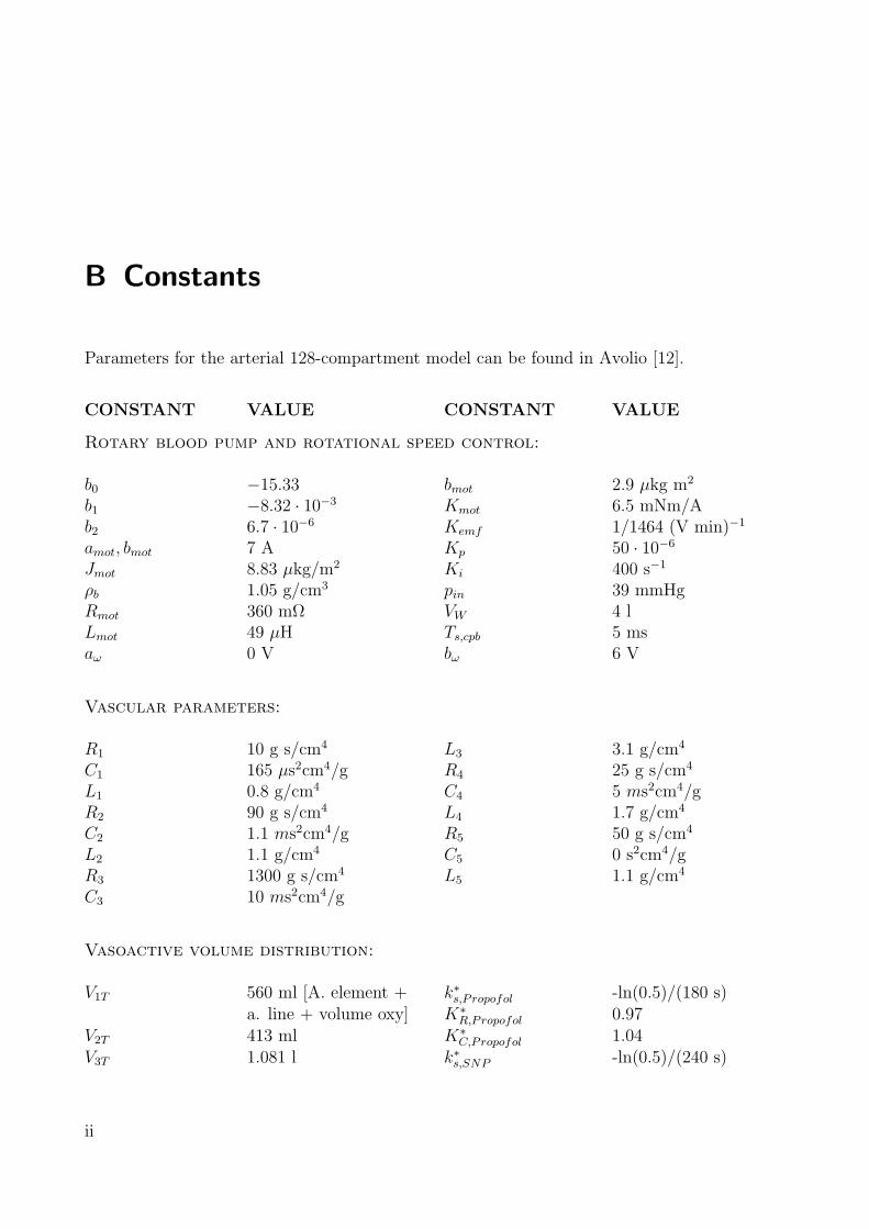
B Constants
Parameters for the arterial 128-compartment model can be found in Avolio [12].
CONSTANT VALUE CONSTANT VALUE
Rotary blood pump and rotational speed control:
b0 −15.33 bmot 2.9 µkg m2
b1 −8.32 · 10−3 Kmot 6.5 mNm/Ab2 6.7 · 10−6 Kemf 1/1464 (V min)−1
amot, bmot 7 A Kp 50 · 10−6
Jmot 8.83 µkg/m2 Ki 400 s−1
ρb 1.05 g/cm3 pin 39 mmHgRmot 360 mΩ VW 4 lLmot 49 µH Ts,cpb 5 msaω 0 V bω 6 V
Vascular parameters:
R1 10 g s/cm4 L3 3.1 g/cm4
C1 165 µs2cm4/g R4 25 g s/cm4
L1 0.8 g/cm4 C4 5 ms2cm4/gR2 90 g s/cm4 L4 1.7 g/cm4
C2 1.1 ms2cm4/g R5 50 g s/cm4
L2 1.1 g/cm4 C5 0 s2cm4/gR3 1300 g s/cm4 L5 1.1 g/cm4
C3 10 ms2cm4/g
Vasoactive volume distribution:
V1T 560 ml [A. element + k∗s,Propofol -ln(0.5)/(180 s)a. line + volume oxy] K∗
R,Propofol 0.97V2T 413 ml K∗
C,Propofol 1.04V3T 1.081 l k∗s,SNP -ln(0.5)/(240 s)
ii

V4T 4.387 l K∗R,SNP 0.975
V5T 1.01 l K∗C,SNP 1
VRT 942.5 ml [V. return]
Oxygenator, Arterial Filter, Tubing and Catheter:
Roxy 477.12 g/(cm4 s) Loxy 56.56 g/cm4
Coxy 10.35 µs2cm4/g Rfil 107.74 g/(cm4 s)Cfil 1.12 µs2cm4/g Rtub 107.74 g/(cm4 s)Ltub 66.8 g/cm4 aC1 4.44 g/(cm7 s)aC0 16 g/(cm4 s) Lcath 10.4 g/cm4
Hydrodynamic Vascular System Simulator:
Ts,1 10 ms Ts,MOCK 540 msTs,2 100 ms fgm 15 Hz
Gas blender:
Tg,b 0.3 s lt,oxy 2 mdt,oxy 5 mm
Oxygenator:
Vg 0.1 l ku 120 ms−1
Vb 0.25 l kv 89 s−1
pbar 760 mmHg ka 5 kM−1s−1
DO2,m 11.291 µl/(mmHg s) kzo 8.4 nMDCO2,m 414.64 µ l/(mmHg s) kzr 72 nMa1 -8532 cat 13·10−3
a2 2121 αO2 1.35 mM/mmHga3 -67.07 αCO2 3 mM/mmHga4 936·10−3 βpl 6 mM/pHa5 -31.35·10−3 βrbc 57.7 mM/pHa6 2.396·10−3 τrbc 1 msa7 −67.10 τHCO3 200 msk 559 · 10−6 M TpH 100 ms
iii

B Constants
Oxygenator venous input conditions:
[O2]b 6.8 mM [HCO3]pl 26.3 mMpO2,b 40 mmHg [HCO3]rbc 18.2 mM[CO2]pl 1.38 mM r 0.69pCO2,pl 46 mmHg [H]pl 42.3 mM[CO2]rbc 1.38 mM [H]rbc 61 nMpCO2,rbc 46 mmHg [carb] 2.35 mM
Blood-gas analyser:
TBGA 20 s dt,BGA 2 mmTs,BGA 6 s at1 0.05 (min m3)/(l s)Aq 1 mmHg at0 16.667·10−6
lt,BGA 1 m
Blood-flow control:
Kp,BFC 150·10−3 Ts,PI 10 msKi,BFC 8 s−1 aR 0 V (≈ 0 R/min)bR 2 V (≈ 10000 R/min) φGPC 0.1rv 0.1 Rw diag(1, 1, 100, 1000)hp 1 hc 1
Arterial Pressure Control:
Kp,BPC 30·10−3 Ts,PI 10 msKi,BPC 2.41 s−1 aR 0 VbR 2 V
Arterial Pressure Boundary Control:
TLPP 318.3 ms kg 1/80kqb 5 mmHg/(l/min) cg 50 mmHgcqb 3 l/min Ts,PI 10 msKp,PBC 50·10−3 Ki,PBC 0.714 s−1
km 5
Blood-gas control:
β3 1 km2 2.5
iv

β2 0.75 αm2 0.08β1 0.1875 βm2 0.4β0 0.0156 kp1 0.5α0 0.125 αp1 0.06αw0 27/1000 Tδ 5 sβw3 1 kCO2 -8βw2 9/10 TCO2 25βw1 27/100 Tt,CO2 5-10 sβw0 27/1000 aO2 0bO2 ∞ aCO2 0.5 l/minbCO2 7 l/min kp0,O2 0.05kI,O2 0.12 s−1 kp0,CO2 -0.05kI,CO2 0.11 s−1
v
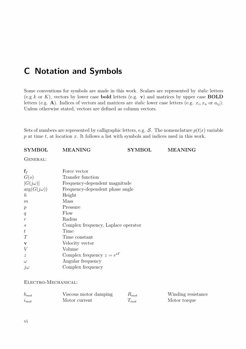
C Notation and Symbols
Some conventions for symbols are made in this work. Scalars are represented by italic letters(e.g k or K), vectors by lower case bold letters (e.g. v) and matrices by upper case BOLDletters (e.g. A). Indices of vectors and matrices are italic lower case letters (e.g. xi, xn or aij).Unless otherwise stated, vectors are defined as column vectors.
Sets of numbers are represented by calligraphic letters, e.g. S. The nomenclature p(t|x) variablep at time t, at location x. It follows a list with symbols and indices used in this work.
SYMBOL MEANING SYMBOL MEANING
General:
ff Force vectorG(s) Transfer function|G(jω)| Frequency-dependent magnitudearg(G(jω)) Frequency-dependent phase angleh Heightm Massp Pressureq Flowr Radiuss Complex frequency, Laplace operatort TimeT Time constantv Velocity vectorV Volumez Complex frequency z = esT
ω Angular frequencyjω Complex frequency
Electro-Mechanical:
bmot Viscous motor damping Rmot Winding resistanceimot Motor current Tmot Motor torque
vi

J Inertia uemf Back electro-magneticKemf Back EMF constant field (EMF) voltageKmot Motor torque constant uin Input voltageLmot Motor inductance ωmot Rotational motor speed
Haemodynamics:
C Vascular compliancec∗n Substance concentration of compartment nCn Fluid compliance of compartment ndn Diameter of vessel, compartment nGvasc(s) Vascular transfer functionJcl Inertia of a cylinderJco Inertia of a truncated conek∗s Half-life time constant of vasoactive substanceL Fluid inertanceLn Fluid inertance of compartment nmcy Mass cylindermco Mass truncated coneqb Blood-flowq∗n Substance flow of compartment npCO2 Carbon dioxide partial pressurepO2 Oxygen partial pressurepin Pressure at pump inletpout Pressure at pump outletR Fluid resistanceRC Fluid resistance, cannulaRcath Fluid resistance, catheterrn Radius of vessel, compartment nRn Fluid resistance of compartment nRoxy Fluid resistance, oxygenatorRtub Fluid resistance, tubing systemV ∗
n Substance volume of compartment nVnT Total volume of compartment nVnU Unstressed volume of compartment nxv Longitudinal vascular axisZvasc(jω) Vascular impedanceη Dynamic viscosityν Kinematic viscosityρ Density of bloodτ Shear stress
vii

C Notation and Symbols
blood-Gas:
[C] Concentration of component CD Diffusion constantFiO2 Oxygen fraction in the gasHb HaemoglobinHct Haematocrit valuepO2 Oxygen blood-gas partial pressurepCO2 Carbon dioxide blood-gas partial pressurepO2,g Oxygen gas partial pressurepCO2,g Carbon dioxide gas partial pressureqg Gas flowRi Dehydration term associated to index iS(·) Saturation functionα Solubilityβ Buffer capacityτi Half-life time associated to a certain drug i
Control:
A System matrixb, B Input vector, matrixc, C Output vector, matrixd, D Straight-way scalar, matrixe, e Control error scalar, vectorG(s), G(s) Transfer function, matrixhc Control horizonhp Prediction horizonI Unity matrixkc Control delayKp Proportional gain constantKi Integral gain constantr, r Control reference scalar, vectorrv Noise varianceRw Process noise covariance matrixTs Sampling timeu, u System input scalar, vectorx System state vectory, y System output scalar, vector
θ Estimated parameter vectorφ Kalman gain vectorφGPC Control input cost weighting
viii

Φ Covariance matrix
Math:
n, m, i, j Integer indices, ∈ Z+
C Set of complex numbersCn×m Complex matrix of dimension n×mf(·), f(·) Scalar or vector functionR Set of real numbersRn n-dimensional vector space of real numbersRn×m Real matrix of dimension n×mZ+ Set of non-negative integers∀ For all
INDICES MEANING INDICES MEANING
aort Aorta mot Motorart Arterial m Membraneb Blood n Referring to indexbar Barometric out OutputBGA Blood-Gas Analysis oxy Oxygenatorc Control, controller p Predictioncath Catheter pl Plasma (blood)cl Cylinder rbc Red blood cellsco Cone (erythrocytes)emf Electro-magnetic field ref Referencefil Filter (arterial) s Samplingf Force tub Tubing Systemg Gas v Vascularht Heart vasc Vascularin Input
ix
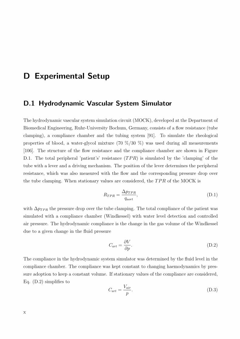
D Experimental Setup
D.1 Hydrodynamic Vascular System Simulator
The hydrodynamic vascular system simulation circuit (MOCK), developed at the Department of
Biomedical Engineering, Ruhr-University Bochum, Germany, consists of a flow resistance (tube
clamping), a compliance chamber and the tubing system [91]. To simulate the rheological
properties of blood, a water-glycol mixture (70 %/30 %) was used during all measurements
[106]. The structure of the flow resistance and the compliance chamber are shown in Figure
D.1. The total peripheral ’patient’s’ resistance (TPR) is simulated by the ’clamping’ of the
tube with a lever and a driving mechanism. The position of the lever determines the peripheral
resistance, which was also measured with the flow and the corresponding pressure drop over
the tube clamping. When stationary values are considered, the TPR of the MOCK is
RTPR =∆pTPR
qaort
, (D.1)
with ∆pTPR the pressure drop over the tube clamping. The total compliance of the patient was
simulated with a compliance chamber (Windkessel) with water level detection and controlled
air pressure. The hydrodynamic compliance is the change in the gas volume of the Windkessel
due to a given change in the fluid pressure
Cart =∂V
∂p. (D.2)
The compliance in the hydrodynamic system simulator was determined by the fluid level in the
compliance chamber. The compliance was kept constant to changing haemodynamics by pres-
sure adoption to keep a constant volume. If stationary values of the compliance are considered,
Eq. (D.2) simplifies to
Cart =Vair
p. (D.3)
x

D.1 Hydrodynamic Vascular System Simulator
DM
L
TS
LE LD
A /Ain out
ACC
BCC
(a) (b)
qb,outqb,in
Figure D.1: Schematic diagram of the hydrodynamic simulation circuit (MOCK) elements. (a) Fluidresistance with driving mechanism DM, the tubing system TS and the lever L. (b) The compliancechamber (Windkessel) with air in- and outflow Ain/Aout, the air in the compliance chamber Acc,the equivalent fluid to blood in the compliance chamber Bcc, the light emitter LE and the lightdetector LD for the level detector.
Both elements, TPR and compliance of the MOCK were adjustable and computer-controlled
and showed almost linear behaviour over the whole operating range [91]. The hydrodynamic
vascular system elements were connected by a tubing system1 (2m length, 3/8’ diameter, 3/32’
wall thickness), which was connected with a HLM, Figure D.2.
To simulate the total cardiopulmonary bypass case with HLM support, the human heart, which
is simulated by another blood pump, was disconnected and the HLM with components oxy-
genator2, arterial filter3 (not shown in Figure D.2) and cannula4 was connected to the MOCK.
A number of additional blood-flow5 and pressure6 sensors were connected to the circuit, for data
recording with the dSpace7 real-time simulation and control environment. The rotary blood
pump8 was connected to the automatic control system (Figure D.2) and the haemodynamic
controllers were initialised in the real-time software for the dSpace environment. The sampling
time for pressure and flow measurement and control with the dSpace control setup was Ts,1 for
the PI- and H∞-controller and Ts,2 for the GPC-controller. Arterial compliance and TPR are
1Tygon, Raumedic, Helmbrechts, Germany2Quadrox, Jostra, Hirrlingen, Germany3Affinity, Medtronic, Minneapolis, USA4TPD 3439, Jostra, Hirrlingen, Germany5T110 flow meter, 9XL flow probe, Transonic Systems Inc., Ithaca, USA6Isotec pressure transducer, TAM-A amplifier, Hugo Sachs Elektronik, Harvard Apparatus GmbH, March-
Hugstetten, Germany7DS1104, dSpace, Paderborn, Germany8DeltaStream, Medos AG, Stolberg, Germany
xi

D Experimental Setup
W
P P PR
VH
PC(parameter
control)
Arterial system
O CP
F
P
BP
P
dSpace control
A
F
Figure D.2: Setup of the hydrodynamic system circuit, with A: dSpace control unit, BP: blood pump,C: cannula, F: flow sensor, H: heart (disconnected, RH →∞), R: total peripheral resistance, O:oxygenator, P: pressure transducer, V: venous system (level-controlled reservoir), W: compliancechamber (Windkessel).
both computer-controlled by a personal computer with AD converter card9 and serial interfaces,
at a sampling time of Ts,MOCK . Arterial compliance and TPR could be changed in the ranges
Cart = [0.8 . . . 2]ml
mmHg
RTPR = [5 . . . 40]mmHg
l/min.
(D.4)
The DeltaStream blood pump was monitored by a driving console and was placed about 40 cm
below the operating table (patient/MOCK). Noisy analogue pressure signals for exact MOCK
control were filtered with a variable filter10 at a 3dB cut-off frequency of fgm. A venous cannula
(not shown in Figure D.2) was implemented in the venous return path of the HLM.
After filling the HLM and the MOCK with the substitute fluid, the whole system was vented.
The controllers were initialised in the real-time code in the dSpace board and haemodynamic
control was started. Over the course of the experiments, the fluid resistance of the oxygenator
and the arterial filter were checked as a matter of routine to detect a partial occlusion of these
components. In the case of any problems they were replaced.
9PCI - 6035, National Instruments, Austin, USA10VDF 8 - 4, Kemo, Inc., Jacksonville, USA
xii

D.2 Pulsatile Control Setpoint
D.2 Pulsatile Control Setpoint
The setpoint for pulsatile control was made out of three variables: Heart rate (HR), mean flow
(MF ) and pulsatility index (PIr). Sinusoidal half-waves with an additionally added DC-part
were used for the blood-flow control reference signal and were determined by MF and HR
(frequency). The pulsatility index PIr determines the ratio of sinusoidal peak value to DC part
flow, refer to Figure D.3. PIr is defined as PIr = A/MF , where A = peak - valley (see Figure
D.3). The given values MF and PI were used to calculate the amplitude A = MF · PI and
the value a0 = MF − A/PI. With these values the pulsatile reference signal is
qb,ref (t) =
A sin(2π·HR
60· t) ∀ 0 < t ≤ T
2
a0 ∀ T2
< t ≤ T. (D.5)
A simple control was implemented in the program to prevent the user from entering values that
would cause unphysiological flows. Also at a given PIr, MF and HR, the pulsatile setpoint
was calculated to satisfy all these values with a flow curve corresponding to the predefined
boundaries (qb = [0 · · · 6] l/min). For that reason, appropriate boundaries for the values in Eq.
(D.5) were defined.
qb [l/min]
time [s]
5
4
3
2
1
00 0.5 1 1.5 2 2.5 3
1/HR
A
Positivesinusoidalhalf wave
MF (mean flow)A/MF=PIr
6
a0
Figure D.3: Pulsatile control setpoint for the arterial blood-flow made out of heart rate (HR), pul-satility index PIr and mean flow MF .
xiii

D Experimental Setup
D.3 In-vitro Blood-Gas Control
For in-vitro evaluation of automatic blood-gas control, the conditions during real CPB were
simulated by use of an artificial blood-gas control circuit [81]. Since the experiments could
neither be accomplished in in-vivo conditions nor with real human blood, the following two
substitutions were made:
- To simulate the highly nonlinear transport capabilities of the human blood, fresh porcine
blood was used as a substitute. Porcine blood has similar haemodynamic and blood-gas
transport properties to human blood [113].
- The blood de-oxygenation and carbonation effect of the human body was simulated by the
use of an oxygenator in de-oxygenation mode with applied nitrogen and carbon dioxide
gas. Since one de-oxygenator cannot remove enough oxygen, three de-oxygenators had to
be used and were connected in series (blood), each having its own gas supply. Nitrogen
and carbon dioxide gases were then controlled to achieve venous conditions of blood-gases.
A detailed description of the in-vitro gas control setup and the materials and methods that
were used follows below.
D.3.1 Experimental Setup
As in the normal total CPB case, the venous return line was connected to an (open) reservoir,
see Figure D.4. From there the deoxygenated carbon dioxide rich blood was pumped through
the oxygenator11 1 and an arterial filter12 back to the simulated patient. The patient was
simulated by means of de-oxygenators 2,3,4, which were connected in series, see Figure D.5.
Blood for the BGA13 was collected directly from the oxygenator (pre-oxygenator = venous
BGA, post-oxygenator = arterial BGA) and was fed back to the reservoir. Pressures in the loop
were measured with pressure sensors14, pre- and post-blood pump15, behind the oxygenator 1
and between oxygenators 2,3,4, and the reservoir. Both gas blenders16 had O2-, CO2- and
11Quadrox, Jostra, Hirrlingen, Germany12Affinity NT Oxygenator, Medtronic, Minneapolis, USA13CDI 500, Terumo, Japan14Isotec pressure transducer, TAM-A amplifier, Hugo Sachs Elektronik, Harvard Apparatus GmbH, March-
Hugstetten, Germany15Deltastream, Medos AG, Stolberg, Germany16GFC 17, Analyt GmbH & CO KG., Mulheim, Germany
xiv

D.3 In-vitro Blood-Gas Control
Oxy 1
Th
erm
osta
t
Pre
ssu
reF
low
Filt
er
Ga
sb
len
de
r 1
BG
A
Re
se
rvo
ir
Blo
od
,p
rim
ing
Ga
sb
len
de
r 2
Oxy´s
2,3
,4(D
e-O
xy)
Oxy 1
Ga
s-
mix
ture
1
Ga
s-
mix
ture
2
Dru
gs
Da
ta s
am
plin
g(X
PC
)
Blo
od
pu
mp
Pre
ssu
reP
ressu
reP
ressu
re
Blo
od
sa
mp
le
Ho
st
PC
(co
ntr
ol)
(a)
Figure D.4: Setup of the blood-gas control circuit with cooling water, blood-gas, arterial and venousline, blood pump, oxygenator, de-oxygenator, reservoir, pressure/flow sensors, thermostat, datasampling unit (XPC Target PC) and Host PC (control). A detailed description of the de-oxygenators (a) is given in Figure D.5.
xv

D Experimental Setup
(a)
Gascompartment
Water in Water in Water in
Water out Water out Water out
qb qb
Gascompartment
Gascompartment
Figure D.5: Serial connection of the three oxygenators in de-oxygenation mode.
N2-gas inputs with automatically controlled gas-flow valves and operating range gas-flow of 0
to 10 l/min. Gas mixtures in each gas mixer could be changed from 0-100 % for each gas.
The blood of the circuit was cooled using a thermostat17 connected to the oxygenators with
water as cooling medium. The blood-gas control circuit elements were connected by a tubing
system18 (2m length, 3/8’ diameter, 3/32’ wall thickness) and additional Luer-Lock connections
were implemented for a drug (pre-oxygenator 1) and a blood sample (post-oxygenator 1) port.
The blood-flow was measured in the arterial line with an ultrasonic flow meter19. A PC with
XPC Target for data collection and control operating at a sampling time of Ts,XPC = 1s was
connected to an AD-converter card20 and communicated with a Host-PC over the serial port.
Data sampling and control were implemented on the Host-PC, where the controllers developed
in Chapter 6 operated with sampling time of the BGA, Ts,BGA = 6s.
D.3.2 Materials and Methods
The fresh porcine blood was collected in a pre-heparinised21 bowl (10000 IU, international
units), directly after regular slaughtering of the pig with high-voltage shock. The collected blood
(about 4-5 l) was bottled and depending on the amount of blood an additional heparin dosage
was applied. The heparin amount was chosen to be around 5000-10000 IU/Litre, where a normal
dosage of 8000 IE/Litre was applied, see sample protocol of an experiment in Table D.1. During
all measurements, additional heparin was applied (if necessary) to keep the active clotting time
(ACT ) above 400 s. The ACT was measured22 every four hours. Before starting the experiment,
17FP 45, JULABO Labortechnik GmbH, Seelbach, Germany18Tygon, Raumedic, Helmbrechts, Germany19T110 flow meter, 9XL flow probe, Transonic Systems Inc., Ithaca, USA20PCL 712PG, Advantech, USA21Heparin-Sodium, Ratiopharm, Ulm, Germany22ACT II, Medtronic, Minneapolis, USA
xvi
D.3 In-vitro Blood-Gas Control
the online BGA control circuit was primed with Ringer-Lactate priming solution23 and reference
measurements were made with a calibration BGA device24. The blood was then applied to the
circuit through a cardiotomy-filter and the circuit was vented. The amount of blood given to
the circuit was calculated using the formula
HctHaem =Vb
Vs + Vb
Hct, (D.6)
with the actual haematocrit value of blood Hct, the desired haematocrit value of the haemo-
diluted fluid HctHaem, the blood volume Vb and the priming solution volume Vs. At a given
haematocrit value and a desired one of e.g. 21 %, Equation D.6 was rearranged to give the
blood volume to
Vb =Vs
HctHctHaem
− 1. (D.7)
Before conducting the BGA control measurements, the base excess (BE) was set to zero, by
the application of sodium hydrogen carbonate25. The gas flows in the de-oxygenators were then
adjusted to agree with venous conditions. This was achieved with the following procedure:
1. An arterial blood-flow rate of qb = 4 l/min was set by the blood pump.
2. The gas flow rate of the oxygenator 1 was set to a total gas-flow 3 l/min with an O2-
concentration of 21 %. At the same time, the nitrogen gas-flow rates of the three de-
oxygenators were set in order to get an oxygen consumption rate of about 110-130 ml/min
(oxygen flow VO2). This oxygen consumption value corresponds to the total oxygen con-
sumption of a typical patient during anaesthesia with applied hypothermia of 28C [68].
Arterial O2-saturation in these conditions was about 99 %, venous O2-saturation about
72 %.
3. To get a venous CO2-partial pressure of about 46 mmHg, the percentage carbon dioxide
flow of the three de-oxygenators was set to a value of FiCO2 = 15-25 %.
After the procedure, venous conditions (pO2,v ≈ 55 mmHg, pCO2,v ≈ 46 mmHg) were obtained,
but a problem occured when changing the blood-flow. Since a total of three de-oxygenators
is needed to de-oxygenise the venous blood, the high gas-flow dramatically changes pCO2,v
23Ringer-Lactat, B. Braun AG, Melsungen, Germany24ABL 77 Series, Radiometer Copenhagen, Copenhagen, Denmark25Molar 8.4 % electrolyte concentrate, Serag-Wiessner GmbH & Co. KG, Naila, Germany
xvii

D Experimental Setup
Table D.1: Sample of an in-vitro BGA-control experimental protocol.
Date: 01/02/06 Experiment No. 8
Start time (killing) 6:10 h
Time to removal of blood ≤ 1 min
Initial amount of heparin ≈ 10,000 IU
Amount of blood 5 l
Total amount of heparin ≈ 8,000 IU/l
Start experiment 8:10h
Starting values
Hct: 26 %
Priming volume: 0.5 l
Temperature (Blood): 28 C
ACT: 420 s
Barometric pressure: 760 mmHg
BGA (reference): pO2,a = 31 mmHg, pCO2,a = 54 mmHg,
pH = 7.38
End of experiment 16:00h
Length experiment 7:50h
Ending values
Hct: 14 %
Priming volume: -
Temperature (Blood): 28 C
ACT: 400 s
Barometric pressure: 760 mmHg
BGA (reference): pO2,a = 140 mmHg, pCO2,a = 27 mmHg,
pH = 7.34
at blood-flow changes. In contrast to that, pO2,v does not change very much. This can be
explained by the following two effects.
1. Oxygen in the blood has a much higher binding affinity than carbon dioxide. This is
because of the chemical binding of oxygen to haemoglobin. A large diffusion pressure
xviii

D.3 In-vitro Blood-Gas Control
difference is therefore needed to remove the oxygen from the blood. This is not the case
with carbon dioxide, which is removed at certain lower gas-flows. The de-oxygenators
were therefore vented with carbon dioxide gas (see above).
2. When considering the oxygen and carbon dioxide binding curves as given in Figure 2.3
and 2.5, it becomes clear that the carbon dioxide pressure varies stronger to a change of
content than the oxygen partial pressure. This is due to the shape of the curve at the
venous pO2,v- and pCO2,v-values.
These effects lead to very low carbon dioxide pressures at low blood-flows and higher carbon
dioxide pressures at higher flows. In order to overcome this highly unphysiological side ef-
fect, an open-loop control was proposed which directly changes the FiCO2-value depending on
flow. Measurements of pCO2,v show an almost quadratic relationship between blood-flow and
percentage of carbon dioxide gas-flow to obtain pCO2,v conditions. The open-loop control was
modelled by a fourth order polynomial and implemented in the real-time process control, Figure
D.6. However, even if pCO2,v is controlled in this way, it breaks down for about 20-30 s when
the blood-flow is changed. This is because the change in the blood-flow is a direct disturbance
to the states of the BGA system and reacts directly on the output (with the time-constant of
the BGA device). The control of the new FiCO2-value corrects pCO2,v after these 20-30 s.
2 2.5 3 3.5 4 4.5 5
32
30
28
26
24
22
20
18
FiCO [%]2
q [l/min]B
Figure D.6: Blood-flow - FiCO2 relationship to keep a constant venous carbon dioxide partial pres-sure, approximated for real-time control by a fourth order polynomial.
xix

D Experimental Setup
Right at the beginning of the experiment, a sample of the haemodiluted blood was taken for the
calibration of the blood-gas analysis and for ACT determination. This procedure was repeated
in steady-state blood-gas control conditions during the experiment and at the end of each ex-
periment. The values of the BGA calibration measurements were compared to the values of the
online BGA. During all in-vitro experiments, the temperature gradient between cooling water
and primed blood was kept below 5 C.
The online BGA measurements for automatic control were conducted in the α-stat mode of
the online BGA device (see Section 3.4.2 for details). Before application of the controller,
the MATLAB/Simulink control model was updated with temperature, Hct, etc. values. Dur-
ing experimental in-vitro control measurements, variables were written on hard-disk from the
MATLAB program at different sampling times.
xx

Bibliography
[1] Maxon AG. Ec 22. Data Sheet, April, 2003.
[2] Maxon Motor AG. Maxon motor control. User Manual, July, 2001.
[3] Medos AG. Deltastream. Medos Medizintechnik, Product Information, 2003.
[4] J. Allen, A. C. Fisher, J. D. Gaylor, and A. R. Razieh. Development of a digital adaptive
control system for pO2 regulation in a membrane oxygenator. J. Biomed. Eng., 14(5):404–
11, 1992. 0141-5425 Journal Article.
[5] J. Anbe, H. Nakajima, Y. Ogura, M. Ozeki, T. Mitsuishi, T. Akasaka, and T. Tobi.
Development of a computer-regulated extracorporeal circulation system. Artif. Organs
Today, 2(2):117–125, 1992.
[6] J. Anbe, T. Tobi, H. Nakajima, T. Akasaka, and K. Okinaga. Microcomputer-based
automatic regulation of extracorporeal circulation: A trial for the application of fuzzy
inference. Artif. Organs, 16(5):532–8, 1992. 0160-564x Journal Article.
[7] J. J. E. Angell. The effects of altering mean pressure, pulse pressure and pulse frequency
of the impulse activity in baroreceptor fibres from the aortic arch and right subclavian
artery in the rabbit. J. Physiol., 214:65–88, 1971.
[8] American Heart Association. Heart disease and stroke - statistics 2004 update. 2004.
[9] G. Avanzolini, P. Barbini, and A. Cappello. Comparison of algorithms for tracking short-
term changes in arterial circulation parameters. IEEE Trans. Biomed. Eng., 39(8):861–7,
1992. 0018-9294 Journal Article.
[10] G. Avanzolini, P. Barbini, A. Cappello, and G. Cevenini. Cadcs simulation of the closed-
loop cardiovascular system. Int. J. Biomed. Comput., 22(1):39–49, 1988. 0020-7101
Journal Article.
xxi
Bibliography
[11] G. Avanzolini, P. Barbini, A. Cappello, and M. R. Massai. Sensitivity analysis of the
systemic circulation with a view to computer simulation and parameter estimation. J.
Biomed. Eng., 11(1):43–7, 1989. 0141-5425 Journal Article.
[12] A. P. Avolio. Multi-branched model of the human arterial system. Med. Biol. Eng.
Comput., 18(6):709–18, 1980. 0140-0118 Journal Article.
[13] H. D. Baehr and K. Stephan. Warme- und Stoffubertragung. Springer, Berlin, 1996.
[14] L. Balmer. Signals and Systems. Prentice Hall, London, 1997.
[15] R. Bauernschmitt, E. Naujokat, H. Mehmanesh, S. Schulz, C. F. Vahl, S. Hagl, and
R. Lange. Mathematical modelling of extracorporeal circulation: Simulation of different
perfusion regimens. Perfusion, 14(5):321–30, 1999. 0267-6591 Journal Article.
[16] W. Beitz and K. H. Kuttner. Taschenbuch fur den Maschinenbau. Springer-Verlag, Berlin
- Heidelberg - New York, 1995.
[17] T. Beppu, Y. Imai, and Y. Fukui. Computer-controlled cardiopumonary bypass system.
Systems and Computers in Japan, 23(11):74–84, 1992.
[18] T. Beppu, Y. Imai, and Y. Fukui. A computerized control system for cardiopulmonary
bypass. J. Thorac. Cardiovasc. Surg., 109(3):428–38, 1995. 0022-5223 Clinical Trial
Controlled Clinical Trial Journal Article.
[19] R. Berber and C. Kravaris, editors. Nonlinear Model Based Control. Kluwer Academic
Publishers, Dordrecht, 1998.
[20] F. Boschetti, F. M. Montevecchi, and R. Fumero. Virtual extracorporeal circulation
process. Int. J. Artif. Organs, 20(6):341–351, 1997.
[21] H. Brandes, J. M. Albes, A. Conzelmann, M. Wehrmann, and G. Ziemer. Comparison of
pulsatile and nonpulsatile perfusion of the lung in an extracorporeal large animal model.
Eur. Surg. Res., 34(4):321–9, 2002. 0014-312x Journal Article.
[22] G. Cattaneo, A. Strauss, and H. Reul. Compact intra- and extracorporeal oxygenator
developments. Perfusion, 19(4):251–255, 2004.
xxii

Bibliography
[23] S. Choi, J. F. Antaki, R. Boston, and D. Thomas. A sensorless approach to control of a
turbodynamic left ventricular assist system. IEEE Trans. Contr. Sys. Tech., 9:473–482,
2001.
[24] S. Choi, J. R. Boston, D. Thomas, and J. F. Antaki. Modelling and identification of an
axial flow pump. Proc. Am. Control Conference, 4:3714–3715, 1997.
[25] Jr. Clark, J. W., G. R. Kane, and H. M. Bourland. On the feasibility of closed-loop
control of intra-aortic balloon pumping. IEEE Trans. Biomed. Eng., 20(6):404–12, 1973.
0018-9294 Journal Article.
[26] D. W. Clarke, C. Mohtadi, and P. S. Tuffs. Generalized predictive control. Automatica,
23(2):137–160, 1987.
[27] R. de Vroege, P. M. Rutten, C. Kalkman, T. A. Out, P. G. Jansen, L. Eijsman, B. J.
de Mol, and C. R. Wildevuur. Biocompatibility of three different membrane oxygenators:
Effects on complement, neutrophil and monocyte activation. Perfusion, 12(6):369–75,
1997. 0267-6591 Clinical Trial Journal Article Randomized Controlled Trial.
[28] D. E. Dick, J. E. Kendrick, G. L. Matson, and V. C. Rideout. Measurement of nonlinearity
in the arterial system of the dog by a new method. Circ. Res., 22(2):101–11, 1968. 0009-
7330 Journal Article.
[29] A. Doenicke, D. Kettler, W. F. List, J. Radke, and J. Tarnow, editors. Anasthesiologie.
Springer, Berlin, 1995.
[30] J. J. Driessen, H. Dhaese, G. Fransen, P. Verrelst, L. Rondelez, L. Gevaert, M. van
Becelaere, and E. Schelstraete. Pulsatile compared with nonpulsatile perfusion using
a centrifugal pump for cardiopulmonary bypass during coronary artery bypass grafting.
Effects on systemic haemodynamics, oxygenation, and inflammatory response parameters.
Perfusion, 10(1):3–12, 1995.
[31] V. B. Fiedler. Effects of pulsatile and non-pulsatile perfusion on the isolated canine heart.
Res. Exp. Med. (Berl.), 179(3):183–98, 1981. 0300-9130 Journal Article.
[32] W. Forth, D. Henschler, and W. Rummel. Allgemeine und spezielle Pharmakologie und
Toxikologie. Bibliographisches Institut, Mannheim, 1983.
xxiii
Bibliography
[33] P. Francheteau, J. L. Steimer, H. Merdjan, M. Guerret, and C. Dubray. A mathematical
model for dynamics of cardiovascular drug action: Application to intravenous dihydropy-
ridines in healthy volunteers. J. Pharmacokin. Biopharm., 21(5):489–513, 1993.
[34] O. Frank. Die Grundform des arteriellen Pulses. Z. Biol., 37:483–526, 1899.
[35] Y. Fukui, K. Tsuchiya, and Y. Imai. Computer controlled extracorporeal circulation
(ECC) with pulsatile perfusion for an infant. Trans. Am. Soc. Artif. Intern. Organs,
28:133–7, 1982. 0066-0078 Journal Article.
[36] Y. C. Fung. Biomechanics Circulation. Springer, New York - Berlin - Heidelberg, 1997.
[37] C. Gao, A. H. Stammers, R. L. Ahlgren, T. A. Ellis, H. B. Holcomb, B. T. Nutter, R. G.
Schmer, and L. Hock. The effects of preprimed oxygenators on gas transfer efficiency. J.
Extra. Corpor. Technol., 35(2):121–6, 2003. 0022-1058 Journal Article.
[38] J. F. Gardner, M. Ignatoski, U. Tasch, A. J. Snyder, and D. B. Geselowitz. Aortic
pressure estimation with electro-mechanical circulatory assist devices. J. Biomech. Eng.,
115(2):187–94, 1993. 0148-0731 Journal Article.
[39] K. Gersten and H. Herwig. Stromungsmechanik. Vieweg, Braunschweig, 1992.
[40] C. Gobel, A. Arvand, R. Eilers, O. Marseille, C. Bals, B. Meyns, W. Flameng, G. Rau,
and H. Reul. Development of the MEDOS/HIA deltastream extracorporeal rotary blood
pump. Artif. Organs, 25(5):358–65, 2001. 0160-564x Journal Article.
[41] R. J. Gordon, M. Ravin, G. R. Daicoff, and R. E. Rawitscher. Effects of hemodilution on
hypotension during cardiopulmonary bypass. Anesth. Analg., 54(4):482–8, 1975. 0003-
2999 Journal Article.
[42] W. Gundel, G. Cherry, B. Rajagopalan, L. B. Tan, G. Lee, and D. Schultz. Aortic input
impedance in man: Acute response to vasodilator drugs. Circulation, 63(6):1305–14,
1981. 0009-7322 Journal Article.
[43] A. C. Guyton. Textbook of Medical Physiology. W. B. Saunders Company, Philadelphia,
1986.
[44] M. A. Henson and D. E. Seborg. Critique of exact linearization strategies for process
control. J. Proc. Cont., 1:122–139, 1991.
xxiv

Bibliography
[45] D. A. Hettrick, P. S. Pagel, and D. C. Warltier. Differential effects of isoflurane and
halothane on aortic input impedance quantified using a three-element windkessel model.
Anesthesiology, 83(2):361–73, 1995. 0003-3022 Journal Article.
[46] M. Hexamer, B. Misgeld, A. Prenger-Berninghoff, U. Schutt, H. J. Knobl, R. Korfer, and
J. Werner. Automatic control of the extra-corporal bypass: System analysis, modelling
and evaluation of different control modes. Biomed. Technik, 49:316–321, 2004.
[47] M. Hexamer and J. Werner. A mathematical model for the gas transfer in an oxygenator.
In D. Feng and E. Carson, editors, Modelling and Control in Biomedical Systems, pages
409–414, Melbourne, Australia, 2003.
[48] E. P. Hill, G. G. Power, and L. D. Longo. A mathematical model of carbon dioxide
transfer in the placenta and its interaction with oxygen. Am. J. Physiol., 224(2):283–99,
1973. 0002-9513 Journal Article.
[49] E. P. Hill, G. G. Power, and L. D. Longo. Mathematical simulation of pulmonary O2 and
CO2 exchange. Am. J. Physiol., 224(4):904–17, 1973. 0002-9513 Journal Article.
[50] E. P. Hill, G. G. Power, and L. D. Longo. Kinetics of O2 and CO2 exchange. In J. B.
West, editor, Bioengineering aspects of the lung, pages 459–514. Marcel Dekker Inc., New
York and Basel, 1977.
[51] MathWorks Inc. Control System Toolbox. The MathWorks, Natick, Mass., 2002.
[52] MathWorks Inc. Signal Processing Toolbox. The MathWorks, Natick, Mass., 2002.
[53] MathWorks Inc. Robust Control Toolbox. The MathWorks, Natick, Mass., 2004.
[54] S. Isaka and A. V. Sebald. Control strategies for arterial blood pressure regulation. IEEE
Trans. Biomed. Eng., 40(4):353–63, 1993. 0018-9294 Journal Article Review.
[55] A. Isidori, editor. Nonlinear Control Systems. Springer-Verlag, Berlin, 1989.
[56] A. Isidori and C. I. Byrnes. Output regulation of nonlinear systems. IEEE Trans. Au-
tomat. Contr., 35(2):131–140, 1990.
[57] J. A. Jacquez, editor. Compartmental Analysis in Biology and Medicine. University of
Michigan Press, Ann Arbor, 1985.
xxv

Bibliography
[58] D. Jaron, T. W. Moore, and P. He. Control of intraaortic balloon pumping: Theory and
guidelines for clinical applications. Ann. Biomed. Eng., 13(2):155–75, 1985. 0090-6964
Journal Article.
[59] R. E. Kalman. A new approach to linear filtering and prediction problems. ASME - J.
Basic Eng., 82:35–45, 1960.
[60] R. E. Kalman and R. Bucy. New results in filtering and prediction theory. J. Basic Eng.,
83:95–108, 1961.
[61] H. Kaufman, R. Roy, and X. Xu. Model reference adaptive control of drug infusion rate.
Automatica, 20(2):205–209, 1984.
[62] P. H. Kay and C. M. Munsch. Techniques in extracorporeal circulation. Arnold, London,
2004.
[63] G. R. Kelman. Digital computer subroutine for the conversion of oxygen tension into
saturation. J. Appl. Physiol., 21:1375–1376, 1966.
[64] T. Kitamura. Left atrial pressure controller design for an artificial heart. IEEE Trans.
Biomed. Eng., 37(2):164–9, 1990. 0018-9294 Journal Article.
[65] G. K. Klute, U. Tasch, and D. B. Geselowitz. An optimal controller for an electric
ventricular assist device: Theory, implementation and testing. IEEE Trans. Automat.
Contr., 39(4):394–403, 1992.
[66] C. Kravaris and R. A. Wright. Deadtime compensation for nonlinear processes. AIChE
J., 35(9):1535–1542, 1989.
[67] T. W. Latson, W. C. Hunter, N. Katoh, and K. Sagawa. Effect of nitroglycerin on aortic
impedance, diameter, and pulse-wave velocity. Circ. Res., 62(5):884–90, 1988. 0009-7330
Journal Article.
[68] G. Lauterbach. Handbuch der Kardiotechnik. Gustav Fischer Verlag, Lubeck, 1996.
[69] D. Lowe, D. A. Hettrick, P. S. Pagel, and D. C. Warltier. Propofol alters left ventricular
afterload as evaluated by aortic input impedance in dogs. Anesthesiology, 84(2):368–76,
1996. 0003-3022 Journal Article.
xxvi

Bibliography
[70] K. Lu, J. W. Clark, F. H. Ghorbel, D. L. Ware, and A. Bidani. An integrated model
of the human cardiopulmonary system. In Proc. 23rd IEEE Eng. Med. Biol. Soc., pages
412–414, Piscataway, NJ, 2001.
[71] J. Lunze. Regelungstechnik 1. Springer-Verlag, Berlin, 2002.
[72] J. Lunze. Regelungstechnik 2. Springer-Verlag, Berlin, 2002.
[73] J. Lunze. Automatisierungstechnik. Oldenbourg, Munchen, 2003.
[74] S. P. Marlow. A PO2 regulation system for a membrane oxygenator. PhD thesis, Univer-
sity of Strathclyde, 1982.
[75] B. C. McInnis, Z.-W. Guo, P. C. Lu, and J.-C. Wang. Adaptive control of left ventricular
bypass assist devices. IEEE Trans. Automat. Contr., 30(4):322–329, 1985.
[76] S. I. Merz. Automatic Control of Extracorporeal Life Support. PhD thesis, University of
Michigan, 1993.
[77] S. I. Merz, R. H. Bartlett, J. M. Jenkins, and P. T. Kabamba. Controller design for
extracorporeal life support. In Proc. 18th IEEE Eng. Med. Biol. Soc., pages 1733–1735,
Piscataway, NJ, 1996.
[78] B. J. E. Misgeld and M. Hexamer. Modellierung und Regelung des arteriellen Blutflusses
wahrend der extrakorporalen Zirkulation. Automatisierungstechnik, 53(9):454–461, 2005.
[79] B. J. E. Misgeld, J. Werner, and M. Hexamer. Automatic control of extracorporeal
circulation: Arterial blood flow control. Biomed. Technik, 50:857–858, 2005.
[80] B. J. E. Misgeld, J. Werner, and M. Hexamer. Robust and self-tuning blood flow control
during extracorporeal circulation in the presence of system parameter uncertainties. Med.
Biol. Eng. Comput., 43:589–598, 2005.
[81] B. J. E. Misgeld, J. Werner, and M. Hexamer. In-vitro experimental setup for the simu-
lation of blood-gas exchange during cardiopulmonary bypass. Biomed. Technik, 2006.
[82] B. J. E. Misgeld, J. Werner, and M. Hexamer. Nonlinear robust blood gas control by state
linearisation for the cardiopulmonary bypass. Control Eng. Practice, 2006. submitted.
[83] B. J. E. Misgeld, J. Werner, and M. Hexamer. Simultaneous control of O2- and CO2-blood
gases during cardiopulmonary bypass. Biomed. Technik, 2006.
xxvii
Bibliography
[84] B.J.E. Misgeld, J. Werner, and M. Hexamer. Strategies for haemodynamic control of ex-
tracorporeal circulation. In 6th IFAC Symposium on Modelling and Control in Biomedical
Systems, pages 351–356, Reims, France, 2006.
[85] B.J.E. Misgeld, J. Werner, and M. Hexamer. Automatisierung der extrakorporalen
Zirkulation: Ein Vergleich verschiedener Regelansatze. In O. Simanski, editor, Automa-
tisierungstechnische Methoden und Systeme fur die Medizin (AUTOMED), pages 55–56,
Rostock, Germany, 2006.
[86] D. Moeller. Ein geschlossenes nichtlineares Modell zur Simulation des Kurzzeitverhaltens
des Kreislaufsystems und seine Anwendung zur Identifikation. PhD thesis, Universitat
Bremen, Berlin, 1981.
[87] M. Morari and E. Zafiriou. Robust Process Control. Prentice-Hall International, Inc.,
Englewood Cliffs, NJ, 1989.
[88] P. Moreton. Industrial Brushless Servomotors. Reed Educational and Professional Pub-
lishing, Oxford, 2000.
[89] A. Mori, K. Watanabe, M. Onoe, S. Watarida, Y. Nakamura, T. Magara, R. Tabata, and
Y. Okada. Regional blood flow in the liver, pancreas and kidney during pulsatile and
nonpulsatile perfusion under profound hypothermia. Jpn. Circ. J., 52(3):219–27, 1988.
0047-1828 Journal Article.
[90] M. H. Nadjmabadi, H. Rastan, M. T. Saidi, and E. Aftandelian. Hamodynamische Veran-
derungen nach akuter intraoperativer Hamodilution bei offener Herzchirurgie. Anaesthe-
sist, 27(8):364–369, 1978.
[91] M. Nagel. Aufbau eines Versuchsstandes zur Simulation des menschlichen Kreislaufs unter
den Bedingungen der extrakorporalen Membranoxygenation (ECMO). Master’s thesis,
Dortmund University, 2004.
[92] E. Naujokat. Ein Beobachtersystem fur den Patientenzustand in der Herzchirurgie. PhD
thesis, Universitat Karlsruhe, Aachen, 2002.
[93] O. Nelles. Nonlinear System Identification. Springer-Verlag, Berlin, 2001.
[94] N. S. Nise. Control Systems Engineering. Wiley and Sons Inc., New York, 2004.
xxviii

Bibliography
[95] H. Nishida, T. Beppu, M. Nakajima, T. Nishinaka, H. Nakatani, K. Ihashi, T. Katsumata,
M. Kitamura, S. Aomi, M. Endo, and et al. Development of an autoflow cruise control
system for a centrifugal pump. Artif. Organs, 19(7):713–8, 1995. 0160-564x Journal
Article.
[96] A. Noordergraaf, A. P. D. Verdouw, and H. B. C. Boom. The use of an analog computer
in a circulation model. Prog. Cardiovasc. Dis., 5:419–39, 1963.
[97] K. Ogata. Discrete - Time Control Systems. Prentice Hall, Englewood Cliffs, NJ, 1987.
[98] J. M. Orenstein, N. Sato, B. Aaron, B. Buchholz, and S. Bloom. Microemboli observed in
deaths following cardiopulmonary bypass surgery: Silicone antifoam agents and polyvinyl
chloride tubing as sources of emboli. Hum Pathol, 13(12):1082–90, 1982.
[99] M. Oshikawa, K. Araki, K. Nakamura, H. Anai, and T. Onitsuka. Detection of total assist
and sucking points based on the pulsatility of a continuous flow artificial heart: In vivo
evaluation. Asaio J., 44(5):M704–7, 1998. 1058-2916 Journal Article.
[100] M. T. O’Toole, editor. Encyclopedia and Dictionary of Medicine, Nursing and Allied
Health. Saunders, Philadelphia, 2003.
[101] A. D. Pacifico, S. Digerness, and J. W. Kirklin. Acute alterations of body composition
after open intracardiac operations. Circulation, 41(2):331–41, 1970.
[102] C. C. Palerm, B. W. Bequette, and S. Ozcelik. Robust control of drug infusion with time
delays using direct adaptive control: Experimental results. In Proc. Am. Contr. Conf.,
volume 5, pages 2972–2976, Chicago, U.S.A., 2000.
[103] L. De Pater. An Electrical Analogue of the Human Circulatory System. PhD thesis,
University of Groningen, Rotterdam, 1966.
[104] G. Pennati, G. B. Fiore, K. Lagana, and R. Fumero. Mathematical modeling of fluid
dynamics in pulsatile cardiopulmonary bypass. Artif. Organs, 28(2):196–209, 2004.
[105] C. J. Pepine, W. W. Nichols, Jr. Curry, R. C., and C. R. Conti. Aortic input impedance
during nitroprusside infusion. A reconsideration of afterload reduction and beneficial ac-
tion. J. Clin. Invest., 64(2):643–54, 1979. 0021-9738 Journal Article.
[106] H. Reul, H. Minamitani, and J. Runge. A hydraulic analog of the systemic and pulmonary
circulation for testing artificial hearts. Proc. ESAO II, 2:120–127, 1975.
xxix

Bibliography
[107] V. C. Rideout. Cardiovascular system simulation in biomedical engineering education.
Trans. Biomed. Eng., 19(2):101–107, 1972.
[108] V. C. Rideout and D. E. Dick. Difference-differential equations for fluid flow in distensible
tubes. IEEE Trans. Biomed. Eng., 14(3):171–7, 1967. 0018-9294 Journal Article.
[109] W. C. Rose and A. A. Shoukas. Two-port analysis of systemic venous and arterial
impedances. Am J Physiol, 265(5 Pt 2):H1577–87, 1993. 0002-9513 Journal Article.
[110] S. Sastry, editor. Nonlinear Systems. Springer-Verlag, New York, 1999.
[111] H. Schima, J. Honigschnabel, W. Trubel, and H. Thoma. Computer simulation of the
circulatory system during support with a rotary blood pump. ASAIO Trans., 36(3):M252–
4, 1990. 0889-7190 Journal Article.
[112] R. F. Schmidt, G. Thews, and F. Lang, editors. Physiologie des Menschen. Springer,
Berlin, 2000.
[113] K. Schmidt-Nielsen. Animal Physiology. Cambridge University Press, London, 1975.
[114] S. Schulz, R. Bauernschmitt, F. Maar, A. Schwarzhaupt, C. F. Vahl, and U. Kiencke. Mod-
ellierung des Barorezeptorreflexes in einem pulsatilen Modell. Biomed. Techn. (Suppl.),
43:310–311, 1998.
[115] A. Schwarzhaupt. Regelung der extrakorporalen Zirkulation auf der Basis eines Modells
des menschlichen Kreislaufes. PhD thesis, Universitat Karlsruhe, Gottingen, 2002.
[116] A. Schwarzhaupt, B. Qaqunda, and U. Kiencke. Entwurf eines pradiktiven MIMO-Reglers
fur Herz-Lungen-Maschinen auf der Grundlage eines Modells der extrakorporalen Zirku-
lation. Biomed. Tech. (Suppl.), 43:336–337, 1998.
[117] P. Segers, F. Dubois, D. De Wachter, and P. Verdonck. Role and relevancy of a cardio-
vascular simulator. CVE, 3(1):48–56, 1998.
[118] T. Shimooka, Y. Mitamura, and T. Yuhta. Investigation of parameter estimator and
adaptive controller for assist pump by computer simulation. Artif. Organs, 15(2):119–28,
1991. 0160-564x Journal Article.
xxx

Bibliography
[119] B. W. Smith, J. G. Chase, G. M. Shaw, and R. I. Nokes. Experimentally verified mini-
mal cardiovascular system model for rapid diagnostic assistance. Control Eng. Practise,
13:1183–93, 2004.
[120] O. J. M. Smith. Closer control of loops with dead time. Chem. Eng. Progress, 53(3):217–
219, 1957.
[121] M. F. Snyder and V. C. Rideout. Computer simulation studies of the venous circulation.
IEEE Trans. Biomed. Eng., 16(4):325–34, 1969. 0018-9294 Journal Article.
[122] M. F. Snyder, V. C. Rideout, and R. J. Hillestad. Computer modeling of the human
systemic arterial tree. J. Biomech., 1:341–353, 1968.
[123] K. Soejima, Y. Nagase, K. Ishihara, Y. Takanashi, Y. Imai, K. Tsuchiya, and Y. Fukui.
Computer-assisted automatic cardiopulmonary bypass system for infants. In K. Atsumi,
M. Maekawa, and K. Ota, editors, Progr. Artif. Organs, pages 918–922. ISAO Press,
Cleveland, OH, 1983.
[124] Z. Song, C. Wang, and A. H. Stammers. Clinical comparison of pulsatile and nonpulsatile
perfusion during cardiopulmonary bypass. J. Extra. Corpor. Technol., 29(4):170–5, 1997.
0022-1058 Clinical Trial Journal Article Randomized Controlled Trial.
[125] K. M. Sutherland, D. T. Pearson, and L. S. Gordon. Independent control of blood gas
pO2 and pCO2 in a bubble oxygenator. Clin. Phys. Physiol. Meas., 9(2):97–105, 1988.
[126] K. M. Taylor, W. H. Bain, and J. J. Morton. The role of angiotensin II in the development
of peripheral vasoconstriction during open-heart surgery. Am Heart J, 100(6 Pt 1):935–7,
1980. 0002-8703 Journal Article.
[127] K. M. Taylor, W. H. Bain, M. Russell, J. J. Brannan, and I. J. Morton. Peripheral vascular
resistance and angiotensin II levels during pulsatile and no-pulsatile cardiopulmonary
bypass. Thorax, 34(5):594–8, 1979. 0040-6376 Journal Article.
[128] K. M. Taylor, J. J. Brannan, W. H. Bain, P. K. Caves, and I. J. Morton. Role of
angiotensin ii in the development of peripheral vasoconstriction during cardiopulmonary
bypass. Cardiovasc Res, 13(5):269–73, 1979. 0008-6363 Journal Article.
[129] R. J. Tschaut. Extrakorporale Zirkulation in Theorie und Praxis. Pabst Science Publish-
ers, Lengerich, 1999.
xxxi

Bibliography
[130] M. Turina, B. Litchford, I. Babotal, M. Intaglietta, and N. S. Braunwald. Servo-controlled
extended cardiopulmonary bypass. Trans. Am. Soc. Artif. Intern. Organs, 19:504–10,
1973. 0066-0078 Journal Article.
[131] W. Saggau und I. Baca, E. Ros, H. H. Storch, and W. Schmitz. Klinische und expe-
rimentelle Studie uber den pulsatilen und kontinuierlichen Fluß wahrend des extrakorpo-
ralen Kreislaufs. Herz, 5(1):42–50, 1980.
[132] V. Videm, T.E. Mollnes, P. Garred, and J.L. Svennevig. Biocompatibility of extracorpo-
real circulation. In vitro comparison of heparin-coated and uncoated oxygenator circuits.
J. Thorac. Cardiovasc. Surg., 101(4):654–660, 1991.
[133] J. Wada, T. Hino, K. Kaizuka, and W. R. Ade. Automatic regulation of the cardiopul-
monary bypass. Perfusion, 1:117–124, 1986.
[134] P. E. Wellstead and M. B. Zarrop. Self-Tuning Systems. Wiley and Sons Ltd., Chichester,
1991.
[135] C. Welp, J. Werner, D. Boehringer, and M. Hexamer. Ein pulsatiles Herz/Kreislauf-
Modell fur die Herzschrittmachertechnik. Automatisierungstechnik, 50(7):326–333, 2002.
[136] J. Werner, editor. Kooperative und autonome Systeme der Medizintechnik. Oldenbourg,
Munchen, 2005.
[137] J. Werner, D. Bohringer, and M. Hexamer. Simulation and prediction of cardiotherapeu-
tical phenomena from a pulsatile model coupled to the guyton circulatory model. IEEE
Trans. Biomed. Eng., 49(5):430–9, 2002. 0018-9294 Journal Article.
[138] N. Westerhof and A. Noordergraaf. Arterial viscoelasticity: A generalized model. J.
Biomech., 3:357–79, 1970.
[139] J. R. Womersley. An elastic tube theory of pulse transmission and oscillatory flow in
mammalian arteries. WADC Technical Report, pages 56–614, 1957.
[140] G. Wright. The hydraulic power outputs of pulsatile and non-pulsatile cardiopulmonary
bypass pumps. Perfusion, 3:251–262, 1988.
[141] T. Yaginuma, A. Avolio, M. O’Rourke, W. Nichols, J. J. Morgan, P. Roy, D. Baron,
J. Branson, and M. Feneley. Effect of glyceryl trinitrate on peripheral arteries alters left
ventricular hydraulic load in man. Cardiovas. Resarch, 20:153–160, 1986.
xxxii

Bibliography
[142] Y.-C. Yu, J. R. Boston, M. A. Simaan, and J. F. Antaki. Estimation of systemic vascular
bed parameters for artificial heart control. IEEE Trans. Automat. Contr., 43(6):765–778,
1998.
[143] G. Zames. Feedback and optimal sensitivity: Model reference transformations, multiplica-
tive seminorms, and approximate inverses. IEEE Trans. Automat. Contr., 26(2):301–320,
1981.
[144] G. Zames and B. A. Francis. Feedback, minimax sensitivity, and optimal robustness.
IEEE Trans. Automat. Contr., 28(5):585–601, 1983.
[145] K. Zhou, J. C. Doyle, and K. Glover, editors. Robust and Optimal Control. Prentice-Hall,
New Jersey, 1996.
xxxiii

Curriculum Vitae
Personal Details
Name: Berno Johannes Engelbert Misgeld
Date of birth: 22. March, 1979
Place of birth: Euskirchen, Germany
Education
08/1996 - 06/1998: Technical High School, Euskirchen, Germany
Military Service
07/1996 - 05/1999: German Airforce, Fernmelderegiment 122, Cochem, Germany
Academic Education
10/2002 - 10/2003: Master of Science (M.Sc.) in Informatics and Control Engineering
Coventry University, Coventry, U.K.
10/1999 - 10/2003: Diplom Ingenieur (FH) in Electrical Engineering
Specialisation: Automation Engineering
Aachen University of Applied Sciences, Aachen, Germany
Work Experience
since 08/2006: Development engineer for automatic flight control/steering
system engineering at Diehl BGT Defence, Nurnberg, Germany
02/2004 - 07/2006: Research associate at the Department for Biomedical Engineering,
School of Medicine, Ruhr-University Bochum, Bochum, Germany
06/2003 - 09/2003: Master Thesis at TRW LucasVarity, System modelling and control
of electric power steering systems, Birmingham, U.K.
04/2002 - 08/2002: Engineering student research project at HiTec Zang,
Automatic control for bio-chemical reactors, Aachen, Germany