Automatic Detection of Flaws in Recorded Music Using Wavelet Fingerprinting

Ryan Laney

A thesis submitted in partial fulfillment of requirements for the degree of Bachelor of Science in

Physics from the College of William & Mary

Accept for: Bachelor of Science in Physics (Honors)

Advisor: Dr. Mark Hinders

Dr. Charles Perdrisat

Dr. John Delos

Dr. Greg Bowers

April 2011

2

Contents

1 Background 7

1.1 Cylinder Recording and Associated Flaws 7

1.2 Digital Recording and Associated Flaws 8

1.3 Previous Work in Automatic Flaw Detection 9

1.4 Current Work in Automatic Flaw Detection 10

2 Theory 15

3 Wavelet Fingerprinting in MATLAB 19

4 Data and Analysis 21

4.1 Method and Analysis of a Non-Localized Extra-Musical Event (Coughing) 21

4.2 Errors Associated with Digital Audio Processing 26

4.3 Automatic Detection of Flaws in Cylinder Recordings using Wavelet Filtering and Wavelet Fingerprint Analysis 29

4.4 Automatic Detection of Flaws in Digital Recordings using Wavelet Filtering and Wavelet Fingerprint Analysis 40

5 Conclusions and Future Work 49

3

List of Figures 1. An Edison phonograph (left) (http://en.wikipedia.org/wiki/Phonograph). An Edison

wax cylinder (right) (http://en.wikipedia.org/wiki/Phonograph_cylinders). 8

2. Wavelet Fingerprint Tool. Top plot: the entire input waveform. Middle plot: a selected portion of the filtered waveform. Bottom plot: fingerprint of the selected part. 11

3. Precise synchronization of waveforms in Pro Tools. The two axes on top refer to the time in minutes and seconds (top) and samples (bottom). 13

4. Comparing samples for synchronization using our MATLAB audio workstation. This image shows the entire waveform, but we are able to zoom in and verify that they are lined-up. 15

5. A spectrogram of a track we analyzed, created with out MATLAB audio workstation. We show frequency, from 0 to 22.05 kHz, on the y-axis and time on the x-axis. 17

6. Shapes of the coiflet3 wavelet (left) and the haar wavelet (right) 18

7. Wavelet fingerprints of an excerpt generated by the coiflet3 wavelet (top) and haar wavelet (bottom) 18

8. Superimposing recorded errors with a signal in the Pro Tools 9 DAW 21

9. Analyzing the data with the Wavelet Fingerprint Tool 23

10. Comparing Wavelet Fingerprints using the Wavelet Fingerprint Tool (no error present) 24

11. Difference in fingerprint with (bottom) and without (top) coughing 24

12. Comparing many different recorded coughs 25

13. Cross-fade of an acoustic guitar in Pro Tools 9 26

14. Comparing acoustic guitar splices: a correct splice (top), a bad splice (middle), zero data in front of splice (bottom) 27

15. Comparing vocal splices: a correct splice (top), a bad splice (middle), zero data in front of splice (bottom) 28

16. Comparing splices of a live recording: a correct splice (top), a bad splice (middle), zero data in front of splice (bottom) 29

17. Comparing Unedited (top) and Edited (bottom) Cylinder Wave Files using our MATLAB Audio Workstation 30

18. Comparing Wavelet Fingerprints of the data in Figure 17 (between 2,257,600 and 2,258,350 samples): edited data (top), unedited data containing pop (bottom) 31

4

19. Instance of a click at 256,000 samples (between 300 and 400 samples in the fingerprint): edited waveform fingerprint (top) and unedited waveform fingerprint (bottom) 31

20. Instance of a click at 103,300 samples (slightly less than 400 samples in the fingerprint): edited waveform fingerprint (top), unedited waveform fingerprint (bottom) 31

21. Using the error at 2,258,000 samples as our generic flaw, we automatically detected the flaw at 256,500 samples (beginning at 296 samples in the fingerprint) using our flaw detection program. 32

22. Using the coiflet3 wavelet to de-noise the input data, we observed the flaw at 256,500 samples with the haar wavelet (about 400 samples in the fingerprint): filtered edited data (top) and its associated fingerprint (second from top), filtered unedited data (second from bottom) and its associated fingerprint (bottom) 33

23. Using the coiflet3 wavelet to de-noise the input data, we observed the flaw at 103,300 samples with the haar wavelet (about 400 samples in the fingerprint): filtered edited data (top) and its associated fingerprint (second from top), filtered unedited data (second from bottom) and its associated fingerprint (bottom) 34

24. We took the shape in Figure 23 as our generic flaw and automatically detected the error in Figure 22 using our flaw detection program. 35

25. Using wavelet filtering and fingerprinting to find where clicks occur between 192,800 and 193,550 samples: filtered edited data (top) and its associated fingerprint (second from top), filtered unedited data (second from bottom) and its associated fingerprint (bottom) 36

26. Using wavelet filtering and fingerprinting to find where clicks occur between approximately 292,600 and 293,350 samples: filtered edited data (top) and its associated fingerprint (second from top), filtered unedited data (second from bottom) and its associated fingerprint (bottom) 37

27. Match values for the unedited waveform between 292,600 and 293,350 samples and the fork-shaped flaw 39

28. Match values for the edited waveform between 292,600 and 293,350 samples and the fork-shaped flaw 39

29. Two versions of a vocal splice from pitch correction in pro tools: a correct cross-fade (top) and a bad splice (bottom) 41

30. Instance of a splice at 81,600 samples (about 400 samples in the fingerprint): edited waveform (top) and associated fingerprint (second from top), unedited waveform (second from bottom) and associated fingerprint (bottom). Fingerprint created using the haar wavelet. 41

5

31. Using the coiflet3 wavelet to de-noise the input data, we observed the flaw at 81,600 samples with the haar wavelet (about 400 samples in the fingerprint): filtered edited data (top) and its associated fingerprint (second from top), filtered unedited data (second from bottom) and its associated fingerprint (bottom) 42

32. At 117,300 samples, we saw the vocal track stay in the positive region for too long as a result of an unmusical splice, which manifested itself musically as a loud pop. 43

33. Instance of a splice at 117,300 samples (about 400 samples in the fingerprint), with the second through fifth detail coefficients removed using the coiflet3 wavelet: edited waveform (top) and associated fingerprint (second from top), unedited waveform (second from bottom) and associated fingerprint (bottom). Fingerprint created using the haar wavelet. 44

34. Instance of a splice at 117,300 samples (slightly before 400 samples in the fingerprint), with the second through fifth detail coefficients removed as well as the fifth approximation coefficient using the coiflet3 wavelet: edited waveform (top) and associated fingerprint (second from top), unedited waveform (second from bottom) and associated fingerprint (bottom). Fingerprint created using the haar wavelet. 45

35. A bad splice in an electric guitar track as a result of time compression on the data to the left. 46

36. Using haar wavelet to create the fingerprint without any pre-filtering, we observed the flaw at about 567,130 samples (slightly before 400 samples in the fingerprint): filtered edited data (top) and its associated fingerprint (second from top), filtered unedited data (second from bottom) and its associated fingerprint (bottom) 47

37. Using the coiflet3 wavelet to de-noise the input data, we observed the flaw at 81,600 samples with the haar wavelet (between 300 and 400 samples in the fingerprint): filtered edited data (top) and its associated fingerprint (second from top), filtered unedited data (second from bottom) and its associated fingerprint (bottom) 48

6

Abstract This thesis describes the application of wavelet fingerprinting as a technique to analyze

and automatically detect flaws in recorded audio. Specifically, it focuses on time-localized

errors in digitized wax cylinder recordings and contemporary digital media. By taking the

continuous wavelet transform of various recordings, we created a two-dimensional binary

display of audio data. After analyzing the images, we implemented an algorithm to

automatically detect where a flaw occurs by comparing the image matrix against the matrix of a

known flaw. We were able to use this technique to automatically detect time-localized clicks,

pops, and crackles in both cylinders and digital recordings. We also found that while other extra-

musical noises, such as coughing, did not leave a traceable mark on the fingerprint, they were

distinguishable from samples without the error.

7

1 Background 1.1 Cylinder Recording and Associated Flaws

Practical audio recording began in the late 19th century with Thomas Edison’s wax

cylinders (Figure 1). The product of experimentation with tinfoil as a recording medium, wax

was found to be a more viable and marketable method of capturing sound. A performer would

play sound into the recording apparatus, shaped like a horn, and the pressure would increase as

sound traveled down the horn. It would then cause a stylus to etch a groove into the wax mold,

which could be played back. Unfortunately, the material would degrade during playback, and

the recording would become corrupted as the wax eroded. This problem persisted into the

twentieth century, even as the production process continued to improve.1 Among the flaws

produced are time-localized pops and crackles, which often render cylinder recordings

unlistenable. The first step in preserving these cylinders is digitization, because at this point the

recording cannot undergo any further damage. While many cylinders have been digitized, many

of these are not of sufficient commercial value to merit fixing by an engineer. Our project aims

to make this next phase easier. If we can automatically detect where the flaws are in a digitized

recording that make it unlistenable, an engineer will have a much easier time fixing them and the

process will be less expensive. Moreover, if multiple recordings of a particular piece exist, an

engineer can select which one is worth fixing based on which has the least amount of errors.

Thus, more of these historically important recordings will be preserved.

8

Figure 1: An Edison phonograph (left) (http://en.wikipedia.org/wiki/Phonograph). An Edison wax cylinder (right) (http://en.wikipedia.org/wiki/Phonograph_cylinders).

1.2 Digital Recording and Associated Flaws

Flaws associated with digital recording are undoubtedly easier to manage than those in

digitized cylinders. Most recording studios now use digital audio workstations (DAWs) on

computers in conjunction with physical mixing stations, and it is common for audio to be

recorded at bit depths at or above 24 bits and 96 kHz, although this is usually truncated down to

16 bits and 44.1 kHz for commercial production. Unlike the case of digitized cylinders,

engineers have each instrument’s individual track (or tracks) to work with rather than just one

master track. Often this means that a flaw can be isolated to just one track, and a correction on

that level is less musically offensive than altering the master. Common problems which

recording engineers spend hours finding and fixing include bad splices, accidental noises from an

audience, and extra-musical sounds from the performers such as vocal clicks, guitar pick noises,

and unwanted breathing. A time-consuming and monotonous portion of many recording

engineers’ jobs is to go through a track little by little, find these errors, and then correct them.

9

Fortunately, the circumstances of digital recording allow for much easier correction of errors. It

is usually a simple matter to create a “correct” version of a track using various processing

techniques, as the digital realm gives the engineer essentially unlimited room to duplicate,

manipulate, and test different variations. This makes automatic detection of the errors much

easier in most cases.

1.3 Previous Work in Automatic Flaw Detection

Programs do exist for correcting errors in audio at a very fine level. CEDAR

(http://www.cedar-audio.com), commercial audio restoration software, lets the user look at a

spectrogram of the sound and remove unwanted parts by altering the image of the spectrogram.

Even cross-fading and careful equalization in most DAWs can eliminate time-localized clicks,

pops, and splice errors. However, this can be both a time-consuming and expensive process, as

the engineer has to both recognize all the errors in a recording and then figure out how to correct

them. In the music industry this never happens unless the recording is highly marketable in the

first place. Due to financial limitations, many historically important recordings on cylinders,

magnetic tape, other analog media, and even digital media don’t merit a human cleaning. The

time and cost it takes to do this would be greatly reduced with an algorithm that automatically

detects errors. There is no effort on the engineer’s part to find the errors; he simply has to make

the correction at the given time. In addition, if multiple versions of a recording exist, an engineer

could select which one would be worth fixing based on the amount of flaws that require

attention.

Previous work in this field has involved using spectrographic analysis as a basis to de-

noise a signal using the continuous wavelet transform. The Single Wavelet Transform 1-

Dimensional De-Noising toolbox in MATLAB (The MathWorks, Inc.) was used to generate a

10

spectrogram of an input signal followed by the spectrogram of the filtered signal. The

continuous wavelet transform yields coefficients of “approximations” and “details”, or lower

frequencies and higher frequencies, which can be individually modified with a certain gain. In a

sense, this is a type of equalization that relies on a wavelet transform as opposed to a Fourier

transform, as all the coefficients belonging to a certain group will be changed according to their

individual gain.2

Unfortunately, spectrographic analysis was not a very practical tool in automating noise

removal. While it was useful in making individual sections of a recording better, large-scale de-

noising on the recording did not make it more listenable. For a given moment in time, it was

appropriate to kill some of the detail coefficients, while removing them at other moments

actually detracted from the musical quality.

1.4 Current Work in Automatic Flaw Detection

We are using a Graphical User Interface (GUI) in MATLAB implemented by the Non-

Destructive Evaluation lab at the College of William & Mary to display and analyze the wavelet

fingerprint of filtered data (Figure 2). The continuous wavelet transform is used to evaluate

patterns related to frequency and intensity in the music, but the output is not a plot of frequency

intensities over time (like a spectrogram), but rather a 2-dimensional binary image. This is a

viable model because it is much easier to recognize patterns in a binary image than in a

spectrogram, and it’s easier to tell a computer how to look at it. By examining raw and filtered

fingerprints for many variations of a certain type of input, we can make generalizations about

how a flaw in a recording will manifest itself in the wavelet fingerprint.3 The wavelet fingerprint

tool works similarly to MATLAB’s built-in wavelet tool: we input sound data from the

workspace in MATLAB and view it as a waveform in the user interface. Below that, we see a

11

filtered version of the wave file according to the filter parameters, and then the wavelet

fingerprint below that.

Figure 2: Wavelet Fingerprint Tool. Top plot: the entire input waveform. Middle plot: a selected portion of the filtered waveform. Bottom plot: fingerprint of the selected part.

The process of writing a detection algorithm involves several important steps. When

working with digital recordings, we reproduced a given flaw via recording or processing in a

digital audio workstation. Using Avid’s Pro Tools DAW (http://www.avid.com), we recorded

coughs, instrumental sounds, and generated other noises one might find in a recording. We

gathered multiple variations of a type of recorded data from multiple people; it does not reveal

anything if the manifestation of one person’s cough is unique, for instance, because then the

algorithm would only be valid for finding that one error. The amplitude, panning, and reverb of

the error can be edited in Pro Tools and then synchronized in time with the clean audio tracks.

The wave files are then exported separately, imported into a workspace in MATLAB, and

analyzed using the Wavelet Fingerprint Tool. Files are compared against other files containing

12

the same error as well as a control file without the error. We can then filter the waveform using

Fourier or wavelet analysis and examine the fingerprints for patterns and similarities.

When working with cylinder recordings, we took a slightly different approach. In this

case, we did not simply insert an error into a clean recording; the recordings we worked with had

the error to begin with. This lack of control meant that, initially, we did not know exactly what

we are looking for. Fortunately, we have access to files that have been processed through

CEDAR’s de-clicking, de-crackling, and de-hissing system. This does help make the recording

more listenable, but the errors are still present to a smaller degree. The cleaned-up files are also

louder and include the proper fades at the beginning and end of the track. Thus, this process is

somewhat analogous to the mastering process in digital music—the final step in making a track

sound its best. By synchronizing the cleaned-up track with the raw track, we can figure out what

we are looking for in the wavelet fingerprint. The errors that are affected by CEDAR will appear

differently in the edited track, and the rest of the track should manifest itself in a similar way.

However, synchronizing the files can be rather challenging. In a digital audio

workstation, it is relatively simple to get the files lined-up within several hundredths of a second.

At this point, the files will sound like they overlap almost completely, but the sound will be more

“full” due to the delay. However, several hundredths of a second at the industry-standard 44.1

kHz sample rate can be up to about 2,000 samples. Due to the visual nature of the wavelet

fingerprint, we need to get the files synchronized much better than that. Synchronization within

about 100 samples is sufficient.

One method of synchronizing the files is simply to examine them visually in a

commercial DAW. By filtering out much of the non-musical information using an equalization

program, the similarities in the unedited and edited waveforms become clearer. We can continue

13

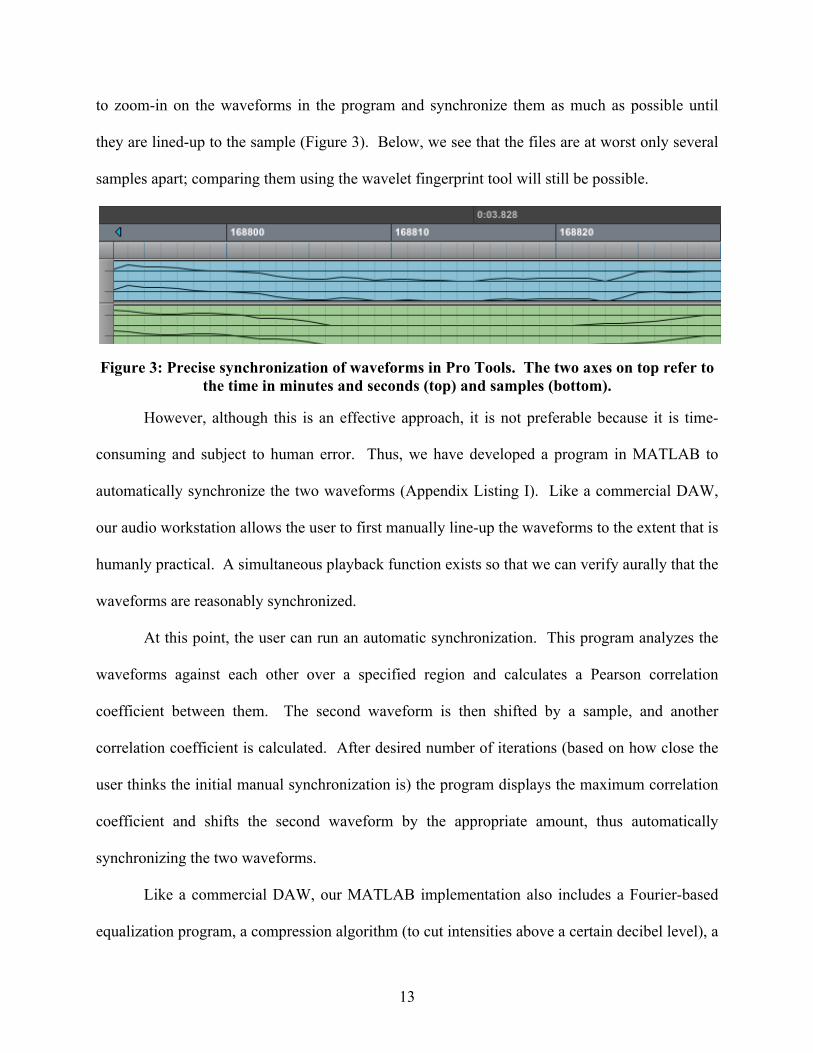
to zoom-in on the waveforms in the program and synchronize them as much as possible until

they are lined-up to the sample (Figure 3). Below, we see that the files are at worst only several

samples apart; comparing them using the wavelet fingerprint tool will still be possible.

Figure 3: Precise synchronization of waveforms in Pro Tools. The two axes on top refer to the time in minutes and seconds (top) and samples (bottom).

However, although this is an effective approach, it is not preferable because it is time-

consuming and subject to human error. Thus, we have developed a program in MATLAB to

automatically synchronize the two waveforms (Appendix Listing I). Like a commercial DAW,

our audio workstation allows the user to first manually line-up the waveforms to the extent that is

humanly practical. A simultaneous playback function exists so that we can verify aurally that the

waveforms are reasonably synchronized.

At this point, the user can run an automatic synchronization. This program analyzes the

waveforms against each other over a specified region and calculates a Pearson correlation

coefficient between them. The second waveform is then shifted by a sample, and another

correlation coefficient is calculated. After desired number of iterations (based on how close the

user thinks the initial manual synchronization is) the program displays the maximum correlation

coefficient and shifts the second waveform by the appropriate amount, thus automatically

synchronizing the two waveforms.

Like a commercial DAW, our MATLAB implementation also includes a Fourier-based

equalization program, a compression algorithm (to cut intensities above a certain decibel level), a

14

gate algorithm (to cut intensities below a certain decibel level), gain control, and a trim function

to change the lengths of a waveform by adding zero values. Unlike most DAWs, however, our

program allows for a more critical examination and alteration of a waveform, including

frequency spectrum analysis by way of a discrete Fourier transform, and spectrograms of the

waveforms.

The equilization tool, while not a paragraphic equalizer, allows for carefully constructed

multi-band rectangular filters to be placed on a waveform after Fourier analysis. This is

particularly helpful in the synchronization process; by removing the low-end of the signal (below

anything that is musically important) and removing the high-end (above any of the fundamental

pitch frequencies, usually no more than several thousand hertz), we can store the unedited and

edited waveforms as temporary variables that end up looking much more like each other than

they did initially. By running the synchronization algorithm on the musically similar temporary

variables, we know exactly how the actual waveforms should match up.

With the unedited and edited files synchronized, we can examine them effectively with

the wavelet fingerprint tool (Figure 4). The more significant differences between the fingerprint

of the unedited sound and that of the edited sound will likely indicate an error. After we

examine multiple instances, if we have enough reason to relate a visual pattern to an audio error,

we can use our detection algorithm to automatically locate a flaw.

15

The detection algorithm we have

implemented involves a numerical evaluation

of the similarity between a known flaw and a

given fingerprint (Appendix Listing II).

Because the wavelet fingerprint is in reality

just a pseudocolor plot of ones and zeros, we

can incrementally shift a smaller flaw matrix

over the larger fingerprint matrix and

determine how similar the two matrices are.

To do this, we simply increase a value

representing how similar the matrices are by a

given amount every time there is a match. The

user is able to decide how many points are

awarded for a match of zeroes and how many

points are awarded for a match of ones. After

the flaw is shifted over the entire waveform

from beginning to end, we plot the match

values and determine where the error is

located. The advantage to this approach is that

it not only points out where errors likely are, but also allows the user to evaluate graphically

where an error might be, incase there is something MATLAB failed to catch.

In using the detection algorithm to analyze audio data, we found that it is often necessary

to increase the width of the ridges and decrease the number of ridges for a reasonable evaluation.

Figure 4: Comparing samples for synchronization using our MATLAB audio workstation. This image shows the entire waveform, but we are able to zoom in and

verify that they are lined-up.

16

Multiple iterations of one error (a pop, for instance) often manifest themselves very differently in

the fingerprint. Thus, it is helpful to have a more general picture of what is happening sonically

from the fingerprint. The match value technique in the detection algorithm gives us an

unrepresentative evaluation of similarity between the given flaw and the test fingerprint if we set

the ridge detail too fine.

2 Theory A Fourier transform is a powerful tool in showing the frequency decomposition of a

given signal. With a given intensity vs. time signal, we can find a set of Fourier coefficients that

when multiplied by a series of sine waves yield the original signal4. These Fourier coefficients

are thus important because they show all frequency components of the spectrum (Equation 1).

€

F(ω ) = f (t)e−iωt dt−∞

∞

∫ (1)

Where F is the frequency vs. intensity representation, f is the original intensity vs. time

signal, and is a complex exponential that can be reduced to its real and imaginary parts.

(Equation 2).

€

F(ω ) = f (t)(cos(ωt) − isin(ωt))dt−∞

∞

∫ (2)

However, the problem with the Fourier transform is that it yields only the frequency vs.

intensity of an intensity vs. time signal. We would like to see frequency, intensity, and time all

in one representation. A spectrogram does meet this criteria—by showing time and frequency on

two axes and intensity with color, we can see what frequencies are present, and how much, at a

given time (Figure 5).5 Programs exist which allow the user to modify the colors in the

17

spectrogram to edit the sound, but spectrograms are difficult to use for automation because the

image is difficult to mathematically associate with a particular type of flaw.

Figure 5: A spectrogram of a track we analyzed, created with out MATLAB audio workstation. We show frequency, from 0 to 22.05 kHz, on the y-axis and time on the x-axis.

A wavelet transform lends itself to our goals much better. Essentially, we calculate the

similarity between a wavelet function and a section of the input signal, and then repeat the

process over the entire signal.6 The wavelet function is then rescaled, and the process is

repeated. This leaves us with many coefficients for each different scale of the wavelet, which we

can then interpret as “approximation” or “detail” coefficients (Equation 3).

€

C = f (t)Ψ(t)dt−∞

∞

∫ (3)

Where f is the original intensity vs. time signal and Ψ is the wavelet, taken at different

scales (up to the length of the input signal) and at different positions along the input signal.

Scale is closely related to frequency, since a wavelet transform taken at a low scale will

18

correspond to a higher frequency component.7 This is easy to understand by imagining how

Fourier analysis works; by changing the scale of a sine wave, we are essentially just changing its

frequency. At this point, we now have a representation of time, frequency, and intensity, all at

once. We can plot the coefficients in terms of time and scale simultaneously. The wavelet

fingerprint tool we have implemented takes these coefficients and creates a binary image of the

signal, much like an actual fingerprint, which is easy for both humans to visually interpret and

computers to mathematically analyze.8 Two of the wavelets we use to a great extent in our

analyses are the coiflet3 wavelet and the haar wavelet, shown below with fingerprints (of the

same excerpt) that they were used to generate (Figures 6 and 7).

Figure 6: Shapes of the coiflet3 wavelet (left) and the haar wavelet (right)

Figure 7: Wavelet fingerprints of an excerpt generated by the coiflet3 wavelet (top) and haar wavelet (bottom)

19

3 Wavelet Fingerprinting in MATLAB The Wavelet Fingerprint tool currently runs from a 650-line code in MATLAB, which we

are continuously modifying for practicality and functionality as it relates to this project. The

function is implemented in a GUI, so users can easily manipulate input parameters. By clicking

on a section of the filtered signal, the user can view the signal’s fingerprint manifestation, and

clicking on the fingerprint will also let the user view what is happening at that point in the signal

to cause that particular realization.

The mathematically interesting part of the code occurs almost exclusively just in the last

hundred lines, where it creates the fingerprint from the filtered waveform. It obtains the

coefficients of the continuous wavelet transform from MATLAB’s built-in cwt function. It

takes the input parameters of the filtered wave from the specified left and right bounds selected

by the user, the number of levels (which is related to scale) to use, and the wavelet to use for the

analysis. This creates a two-dimensional matrix of coefficient values, which are then normalized

to 1 by dividing each component of the matrix by the overall maximum value.9 Initially, the

entire fingerprint matrix is set to the value zero, and then certain areas will be set to one based on

the values of the continuous wavelet transform coefficients, the parameter selected by the user of

how many of these “ridges” there will appear, and how thick they will be. Throughout the

domain of the fingerprint, if the coefficients are greater than the number of ridges minus half

their thickness and less than the number of ridges plus half their thickness, we set the fingerprint

value at that point to be one. This outputs a “fingerprint” whose information is contained in a

two-dimensional matrix. For each fingerprint, the two-dimensional matrix is displayed as a

pseudocolor plot at the bottom of the interface.

20

Several modifications have been made to the original version of this code throughout the

past year. For speed and ease-of-use, this version’s capability to recognize binary or ASCII

input data has been eliminated. We use only data imported into MATLAB’s workspace, so there

is no need to create an error while running the program by accidentally clicking the wrong

button. Several of the program’s default parameters have also been changed. Namely, the

wavelet fingerprint no longer needs to discern between “valleys” (negative intensities) or

“peaks” (positive intensities), because it is only the amplitude of the wave that contains relevant

sonic information. We set a more full 75 “levels” of the wavelet fingerprint by default, rather

than 50, so we can examine all frequencies contained in the data more efficiently. The highest

frequency we can be concerned with is 22.05 kHz, as we cannot take any information from

frequencies higher than half the sampling rate (we always use the industry standard 44.1 kHz).

More practically, the user can now highlight any part of the fingerprint, input signal, or filtered

signal for analysis. The program will still respond even if the user selects left and right bounds

that don’t work, but rather will alter the bounds so that the entire domain shifts over. Titles and

axis labels on all plots of the waveform and the fingerprints are now included as well.

21

4 Data and Analysis

4.1 Method and Analysis of a Non-Localized Extra-Musical Event (Coughing)

To analyze extra-musical events as errors in MATLAB, we generated them artificially

using Pro Tools, and tested many different variations of them with the wavelet fingerprint tool.

Figure 8: Superimposing recorded errors with a signal in the Pro Tools 9 DAW

Figure 8 shows about a 7-second excerpt of a WAV file of Igor Stravinski’s ballet,

Petrouchka. The second track, below that, is a cough. When the file is played back, we can hear

the cough superimposed with the music. In this simulation, the recording is clean, and the error

that we inserted is ultimately what needs to be detected in the signal. We then exported both

tracks together as a WAV file to be used in MATLAB. We always specify WAV file because it

is lossless audio and gives us the best possible digital sound of our original recording. We never

want to experience audio losses due to compression and elimination of higher frequencies in

formats like mp3, despite the great reduction of file size.

The file was then sent to the workspace in MATLAB. By muting the cough, we created a

control file without any extraneous noise and sent that to the workspace in MATLAB as well.

We always exported audio files in mono rather than stereo, because currently the wavelet

22

fingerprint tool can only deal with a single vector of input values rather than two (one each for

left and right). For each file, we renamed the “data” portion of the file, containing the intensity

of the sound at each sample, and remove the “fs” portion, containing the sampling rate (44.1

kHz). This created two files in the workspace: a vector of intensities for the “uncorrupted” file

and a vector for the file with coughing.

When we call the Wavelet Fingerprint Tool in the command window, the loaded

waveform appears above its fingerprint (Figure 9). In the top plot, we see the original waveform.

The second plot shows an optionally filtered (this one is still clean) version of the selected part of

the first plot. The third image shows the fingerprint, in this case created by the coiflet3 wavelet.

The black line on the fingerprint corresponds to the red line on the second plot, so we can see

how the fingerprint relates to the waveform. In the third plot, the yellow areas represent ridges,

or “ones” in the modified wavelet transform coefficients matrix. We can also load the file with

the coughing and examine it in a similar fashion. As a convention, we always set the ridge

number to 15 and ridge thickness to 0.03 for unfiltered data.

23

Figure 9: Analyzing the data with the Wavelet Fingerprint Tool

The code allows us to take a snapshot of all the loaded fingerprints with the “compare

fingerprints” button. This lets us see each of the fingerprints within the most recent bounds of

the middle plot (shown in Figure 9). Purposely, we have selected an area of the fingerprint that

does not contain a cough (Figure 10). There is no visually obvious difference in the fingerprint—

as we expect, if there is no difference in the fingerprint, an error does not exist in this part of the

sample. Shifting the region of interest to a spot with the error (Figure 11), we see in the second

fingerprint that the thumbprint looks very skewed at higher levels. The ridges seem to stretch

significantly further than they did at the lower levels, but their orientation and position is very

much unchanged.

24

Figure 10: Comparing Wavelet Fingerprints using the Wavelet Fingerprint Tool (no error present)

Figure 11: Difference in fingerprint with (bottom) and without (top) coughing

As expected, introducing an error also introduces a difference in the waveform. But now,

we have to test against many other types of errors to determine what the relationship is.

Fortunately, Pro Tools makes it easy to keep track of many different tracks and move sound clips

to the appropriate location in time. We then compared the many different coughing samples in

MATLAB (Figure 12).

25

Figure 12: Comparing many different recorded coughs

While these coughs manifest themselves differently in the music, one similarity we do

notice is an exaggeration of some of the upper-level characteristics in the clean sample (the top

fingerprint). For instance, in most variations, we notice a distortion in the “hook” that occurs at

500 samples around level 50. While this observation is vague, it is still somewhat significant,

since these samples are taken from different “types” of coughs and from different people.

Unfortunately, after testing the same coughing samples against several different audio

recordings, the fingerprints did not show sufficient visual consistency. Although these results

are inconclusive, we think that if we filter the track in some ideal way in future studies, we

26

should be able to identify where a cough might likely occur. The rest of our analysis focuses on

more time-localized errors.

4.2 Errors Associated with Digital Audio Processing

In mixing music, if an engineer wants to put two sounds together in immediate sequence,

he lines them up next to each other in a DAW and cross-fades each portion with the other over a

short time span (Figure 13). One signal fades out while the other fades in. When this is done

incorrectly, it can leave an awkward jump in the sound that sometimes manifests itself as an

audible and very un-musical popping noise. For this analysis, we worked with three different

types of music one might have to splice in the studio: tracks of acoustic guitar strumming, vocal

takes spliced together, and the best takes of recorded audio from a live performance spliced

together (which is very useful if there are multiple takes and the performers mess some of them

up).

Figure 13: Cross-fade of an acoustic guitar in Pro Tools 9

First, we examined chord strumming recorded by an acoustic guitar. One part of a song

was recorded, and then the second part was recorded separately, and the two pieces were put

together. The three plots in Figure 14 show the track spliced together correctly, at a musically

acceptable moment with a brief cross-fade, followed by two incorrect tracks, which are missing

the cross-fade. The last track even has the splice come too late, so there is a very short silence

27

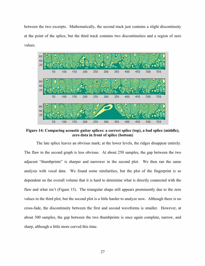
between the two excerpts. Mathematically, the second track just contains a slight discontinuity

at the point of the splice, but the third track contains two discontinuities and a region of zero

values.

Figure 14: Comparing acoustic guitar splices: a correct splice (top), a bad splice (middle), zero data in front of splice (bottom)

The late splice leaves an obvious mark; at the lower levels, the ridges disappear entirely.

The flaw in the second graph is less obvious. At about 250 samples, the gap between the two

adjacent “thumbprints” is sharper and narrower in the second plot. We then ran the same

analysis with vocal data. We found some similarities, but the plot of the fingerprint is so

dependent on the overall volume that it is hard to determine what is directly connected with the

flaw and what isn’t (Figure 15). The triangular shape still appears prominently due to the zero

values in the third plot, but the second plot is a little harder to analyze now. Although there is no

cross-fade, the discontinuity between the first and second waveforms is smaller. However, at

about 300 samples, the gap between the two thumbprints is once again complete, narrow, and

sharp, although a little more curved this time.

28

Figure 15: Comparing vocal splices: a correct splice (top), a bad splice (middle), zero data in front of splice (bottom)

Finally, to work ensemble playing into our analysis, we chose to examine a performance

of an original composition for piano, guitar, percussion, and tenor saxophone (Figure 16). This

piece was performed at a reading session, so splicing together different parts of the piece from

the best takes is what made the complete recording; a full-length, un-spliced recording does not

exist. Once again, in the third plot, we see the characteristic triangle shape. In the upper plots,

however, there is little difference, but there is a slight sharpening of the gap right after 300

samples in the second pot. While this result certainly is helpful, it is probably not code-able,

since sharpness of a gap is not an artifact unique to not cross-fading. However, the presence of

similar visual patterns confirmed that investigating splices further was necessary. Refer to

section 4.4 for a continued analysis of splice errors and detection.

29

Figure 16: Comparing splices of a live recording: a correct splice (top), a bad splice (middle), zero data in front of splice (bottom)

4.3 Automatic Detection of Flaws in Cylinder Recordings using Wavelet

Filtering and Wavelet Fingerprint Analysis

Using files from the University of California at Santa Barbara’s Cylinder Conservation

Project, we compared the fingerprints of unedited and edited digitized cylinders using the

Wavelet Fingerprint tool. The files provided were in stereo, but in actuality are the same in both

the left and right channel, because stereo sound did not exist in cylinder recording. So, we

converted the files to mono by taking only the left channel’s data. As before, the unedited file

and edited file are each a vector the length of the waveform in samples.

Because a complete song is millions of samples long, it is impractical for the wavelet

fingerprint program to process all the data at once. Thus, we examined the complete audio file

using our digital audio workstation implemented in MATLAB to look for more specific spots we

wanted to check for errors (Figure 17). The file on the bottom has been decreased by twelve

decibels so that it looks similar to the first file (for visually accurate comparison). Evidently,

CEDAR’s de-clicking program did a relatively good job getting rid of the many of the louder

clicks, but they still affect the sound in a less overbearing way. We chose two regions to

30

examine with the wavelet fingerprint tool: two million to three million samples, and one to one

million samples.

Figure 17: Comparing Unedited (top) and Edited (bottom) Cylinder Wave Files using our

MATLAB Audio Workstation

We compared several fingerprints of clicks in the unedited waveform with the

fingerprints of the edited waveform. We used a relatively large ridge width of 0.1 and 20 ridges

so we could look for more general trends in the fingerprint (Figure 18). At about 2,258,000

samples, we found a noticeable difference in the two images. The flower-like shape that occurs

at about 400 samples is common in other instances of clicks as well. From about 256,000-

256,750 samples (Figure 19) and about 103,300 samples (Figure 20), we observed a similar

shape. We found that this particular manifestation was more visually apparent when the

musically important information is quieter than the noise.

31

Figure 18: Comparing Wavelet Fingerprints of the data in Figure 17 (between 2,257,600 and 2,258,350 samples): edited data (top), unedited data containing pop (bottom)

Figure 19: Instance of a click at 256,000 samples (between 300 and 400 samples in the fingerprint): edited waveform fingerprint (top) and unedited waveform fingerprint

(bottom)

Figure 20: Instance of a click at 103,300 samples (slightly less than 400 samples in the fingerprint): edited waveform fingerprint (top), unedited waveform fingerprint (bottom)

32

We then chose a flaw to use as the control. We compared this against a larger segment of

the wavelet fingerprint, and using our automatic flaw detection algorithm, found the exact

location of the error. Taking the first error to generate our generic pop fingerprint, we store the

area from 400 to 450 samples in a 75 x 50 matrix. This was shifted over the entire test

fingerprint, counting only the values of the ridges that match, as we can see by looking at the

fingerprint the placement of the zero values do not seem to have much consistency between each

shape. Assigning one match point for each ones match and no points for each zeros match, the

program detected the flaw slightly early at 296 samples (Figure 21). However, it is very visually

apparent that the flaw most likely occurs in the neighborhood of 300 samples, so it did a

reasonably good job of locating it.

Figure 21: Using the error at 2,258,000 samples as our generic flaw, we automatically detected the flaw at 256,500 samples (beginning at 296 samples in the fingerprint) using our

flaw detection program.

We expanded on this method further by filtering the waveform before the fingerprint was

created. Creating a temporary variable from the original waveform revealed useful information

about where important events are located in the waveform. Using the coiflet3 wavelet as our de-

33

noising wavelet, we removed the third through fifth approximation coefficients as well as the

second through fifth detail coefficients on the above excerpts. We found that while much of the

musical information is lost, information about where the errors occurred was exaggerated. At

256,500 samples, we observed a prominent fork shape in the unedited fingerprint (Figure 22). In

taking this data we normalized each fingerprint individually due to the large difference in

intensities between the filtered versions of the clean and unedited wave files. We observed the

same shape at 103,300 samples (Figure 23). For all filtered data, we use a ridge number of 20

and thickness of 0.05.

Figure 22: Using the coiflet3 wavelet to de-noise the input data, we observed the flaw at 256,500 samples with the haar wavelet (about 400 samples in the fingerprint): filtered

edited data (top) and its associated fingerprint (second from top), filtered unedited data (second from bottom) and its associated fingerprint (bottom)

34

Figure 23: Using the coiflet3 wavelet to de-noise the input data, we observed the flaw at 103,300 samples with the haar wavelet (about 400 samples in the fingerprint): filtered

edited data (top) and its associated fingerprint (second from top), filtered unedited data (second from bottom) and its associated fingerprint (bottom)

Taking this feature as our representative pop sample, we counted the number of zeros and

ones in the first fingerprint that match up to see if we can automatically locate it. Our program

caught the flaw perfectly at about 350 samples (Figure 24). The weakness of using this method

is that it appears more likely, for instance, that there is a flaw at zero samples than at 300

samples. For a more accurate search, we need to develop a method that does not count the zero

matches unless there is a significant amount of ones matches.

35

Figure 24: We took the shape in Figure 23 as our generic flaw and automatically detected the error in Figure 22 using our flaw detection program.

Interestingly, we found that while it is difficult to locate the crackling noise made by

cylinders just by looking at the waveform, we believe that we can successfully identify many

instances through the same filtering process. Since these are so widespread throughout the

unedited waveform, we simply selected a portion of the file and examined the fingerprint for the

above shape. For instance, we chose the region at approximately 192,800-193,550 samples in

the same file (Figure 25) and saw less-defined fork shapes appear frequently in the edited

waveform than the unedited waveform. At about 292,000 samples we observed a similar pattern

(Figure 26).

36

Figure 25: Using wavelet filtering and fingerprinting to find where clicks occur between 192,800 and 193,550 samples: filtered edited data (top) and its associated fingerprint

(second from top), filtered unedited data (second from bottom) and its associated fingerprint (bottom)

37

Figure 26: Using wavelet filtering and fingerprinting to find where clicks occur between approximately 292,600 and 293,350 samples: filtered edited data (top) and its associated

fingerprint (second from top), filtered unedited data (second from bottom) and its associated fingerprint (bottom)

38

While both fingerprints contain the fork shape throughout, they are more defined in the

unedited waveform. Since the forks seem to correspond to intensity extremes when they are

well-defined, we think that this means they relate to the degree of presence of the crackling

sounds. Unfortunately, our algorithm for locating these forks is of little use in this situation. We

need a program to count the number of occurrences of forks,rather than individual points, per a

certain number of samples. When we run the fingerprint through the algorithm we already have,

our results are only reasonable. We assign match points for both ones and zeros so that we can

account for how defined the fork shapes are. Figure 27 shows the relative likelihood of a flaw in

the unedited waveform, and Figure 28 shows the same for the edited waveform. We see that in

Figure 27, the peaks in the match values are higher than in Figure 28, suggesting that there is

more crackling present in the unedited version.

39

Figure 27: Match values for the unedited waveform between 292,600 and 293,350 samples and the fork-shaped flaw

Figure 28: Match values for the edited waveform between 292,600 and 293,350 samples and the fork-shaped flaw

40

4.4 Automatic Detection of Flaws in Digital Recordings using Wavelet Filtering and Wavelet Fingerprint Analysis

A common issue in editing is the latency of the cross-fade between splices. For example,

it is often necessary for an engineer to go through vocalists’ recordings and make sure everything

is in tune. This can be fixed in a DAW by selecting the part of the file that is out of tune and

simply raising or lowering its pitch. However, an extraneous noise such as a click or pop may be

created from a change in the waveform. There might be a discontinuity, or the waveform may

stay in the positive or negative region for too long. Oftentimes an automatically generated cross-

fade will not solve the problem, so an engineer needs to go through a recording, track by track,

and listen for any bad splices. Moreover, after the problem is located, the engineer must make a

musical judgment on how to deal with it. The cross-fade cannot be too long, or the separate

regions will overlap, and filtering only a portion of the data could make the sound too strange.

However, using wavelet filtering and fingerprinting comparison techniques, it is simple to

automatically locate bad splices that require additional attention.

In Pro Tools, simulating this is straightforward. We took the vocal track from a

recording session and fully examined it, finding and correcting all the pitch errors. Then, we

listened to the track for any sort of error that resulted from the corrections. We duplicated the

corrected track, and at each instance of an error, manually fixed it on the control track (Figure

29). The track was exported from Pro Tools and examined using the Wavelet Fingerprint Tool

(Figure 30). Fortunately, since we were working in the digital realm, we already knew exactly

where the flaws were, and there was no need to use our audio workstation to automatically sync

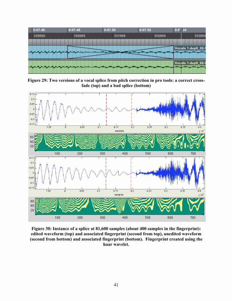
the two tracks. At about 81,500 samples, we see a very distinct image corresponding to the flaw:

a discontinuity in the waveform that sounds like a small click.

41

Figure 29: Two versions of a vocal splice from pitch correction in pro tools: a correct cross-fade (top) and a bad splice (bottom)

Figure 30: Instance of a splice at 81,600 samples (about 400 samples in the fingerprint): edited waveform (top) and associated fingerprint (second from top), unedited waveform (second from bottom) and associated fingerprint (bottom). Fingerprint created using the

haar wavelet.

42

The unedited waveform, unlike the control, has a triangular feature in the middle of the

fingerprint. Removing the fifth approximation coefficient using the coiflet3 wavelet as well as

the second through fifth detail coefficients, however, reveals a very distinct fork shape (Figure

31). We already know from our analysis of cylinder flaws that it is possible to code for this

shape. In one way, this is a very good thing, because it means that this shape, when it is well-

defined, is indicative of a flaw and a computer has a relatively easy time finding it. However, it

does not say much about which particular type of flaw it is. For that information, we need to rely

on the appearance of unfiltered or less filtered data.

Figure 31: Using the coiflet3 wavelet to de-noise the input data, we observed the flaw at 81,600 samples with the haar wavelet (about 400 samples in the fingerprint): filtered edited data (top) and its associated fingerprint (second from top), filtered unedited data (second

from bottom) and its associated fingerprint (bottom)

43

At 117300 samples, we observed another error from pitch correction, this time a loud

pop. The waveform stays in the positive region for too long as a result of the splicing (Figure

32). By filtering out the second through fifth detail coefficients using the coiflet3 wavelet, we

noticed that while the error is visually identifiable in the fingerprint, it is a different type of error

than the previous one we examined (Figure 33). Adding the fifth approximation coefficient to

the filter, we see the characteristic fork shape once again (Figure 34). Once more, the heavy

filtering with the coiflet3 wavelet successfully marked an error, but we cannot say from the

fingerprint exactly what kind of error it is.

Figure 32: At 117,300 samples, we saw the vocal track stay in the positive region for too long as a result of an unmusical splice, which manifested itself musically as a loud pop.

44

Figure 33: Instance of a splice at 117,300 samples (about 400 samples in the fingerprint), with the second through fifth detail coefficients removed using the coiflet3 wavelet: edited waveform (top) and associated fingerprint (second from top), unedited waveform (second

from bottom) and associated fingerprint (bottom). Fingerprint created using the haar wavelet.

45

Figure 34: Instance of a splice at 117,300 samples (slightly before 400 samples in the fingerprint), with the second through fifth detail coefficients removed as well as the fifth

approximation coefficient using the coiflet3 wavelet: edited waveform (top) and associated fingerprint (second from top), unedited waveform (second from bottom) and associated

fingerprint (bottom). Fingerprint created using the haar wavelet.

46

Next, we analyzed the fingerprint of an electric guitar run through a time compression

program (Figure 35). An engineer would need to change how long a note or group of notes lasts

if a musician was not playing in time, but like with pitch corrections, this can result in flaws. We

found that although the instrument is completely different, the error manifests itself in a similar

way in the wavelet fingerprint. At about 567,130 samples, there is a discontinuity in the

waveform resulting from the time compression (to the left). We made a control track by cross-

fading the contracted and normal sections of the waveform, and analyzed the differences in the

wavelet fingerprint in MATLAB. Using the haar wavelet to generate the fingerprint without any

pre-filtering, we found that a triangular figure manifests itself in the middle of the fingerprint

where the splice occurs (Figure 36). This “discontinuity” in the fingerprint was not apparent in

that of the control track.

Figure 35: A bad splice in an electric guitar track as a result of time compression on the data to the left.

47

Figure 36: Using haar wavelet to create the fingerprint without any pre-filtering, we observed the flaw at about 567,130 samples (slightly before 400 samples in the fingerprint): filtered edited data (top) and its associated fingerprint (second from top), filtered unedited

data (second from bottom) and its associated fingerprint (bottom)

48

Next, we used the coiflet3 wavelet to filter the waveform (Figure 37). We killed the fifth

approximation coefficient as well as the second through fifth detail coefficients, and we found

the typical pronounced fork shape occurred at the discontinuity in the waveform. In the

fingerprint of the control waveform, we saw that there was a lack of clarity between each fork,

and the forks themselves were once again not well defined. Although the cause of the

discontinuity was different in this test, it manifested itself in the fingerprint the same way. Thus,

we were able to identify that it is a discontinuity error as well as its location in the sample.

Figure 37: Using the coiflet3 wavelet to de-noise the input data, we observed the flaw at 81,600 samples with the haar wavelet (between 300 and 400 samples in the fingerprint):

filtered edited data (top) and its associated fingerprint (second from top), filtered unedited data (second from bottom) and its associated fingerprint (bottom)

49

5 Conclusions and Future Work

Wavelet fingerprinting proved to be a useful technique in portraying and detecting time-

localized flaws. We were able to very accurately and effectively detect pops and clicks in both

digital recordings and digitized cylinders through a process of filtering the input waveform and

analyzing the fingerprint. Our algorithm precisely located at what point on the wavelet

fingerprint the flaw began and provided a useful graphical display of the relative likelihood of an

error. We found that the same algorithm could be used to detect many manifestations of the

same flaw. Whether it was produced by a bad splice from placement, tuning, or tempo

adjustment, or induced by cylinder degradation, we were able to find where the problem

occurred. While our filtering process and algorithm did not tell us exactly what type of error

occurred or how prominent it was, analysis of the unfiltered fingerprint did reveal a visual

difference between flaws.

Wavelet fingerprinting proved relatively inefficient in detecting flaws in coughs. We

think that because events like this are more sonically diverse in nature and less time-localized, it

was not possible for us to create an automatic detection algorithm. With a high level of filtering,

it may be possible in future work to locate such errors. We also hope in future studies to further

develop a method of detecting less audible flaws, such as the supposed crackles we noticed in

cylinder files, with a higher mathematical level of precision and certainty. We look to extend our

program’s reach to musical flaws such as vocal clicks and the sound of a guitarist’s pick hitting a

fingerboard. Such a tool would be invaluable for engineers in both audio restoration and digital

mastering.

There are several steps we must take to fully apply wavelet fingerprinting as an error

detection technique. First, we must modify our algorithm to search entire tracks for errors and

50

display every instance where one occurs, rather than just the several hundred samples where it

most likely occurs. We can do this essentially by placing intensity marks (for instance, a color or

a number) at every point along the waveform indicating how likely it is that an error occurs

there. When searching for one given type of error, we suspect that these intensity marks will

spike at the points of occurrence. Furthermore, we must modify our algorithm to accurately

detect flaws based on the type of flaw it is. This involves inventing a more flexible and

empirical method of detecting a flaw; this could mean not necessarily looking at all levels of the

fingerprint, allowing uncertainty in how close matching points are, contracting or expanding the

flaw matrix, or assigning match points more liberally or conservatively. It will be a challenge,

but also very necessary, to make our algorithms more adaptive as we continue to investigate

more flaws and improve our current detection methods.

51

Appendix: Programs Implemented in MATLAB

Listing I: Digital Audio Workstation

%% MATLAB Digital Audio Workstation % created by Ryan Laney % 2011 function DAW fprintf('This program allows the user to manipulate, compare, and listen to edited and unedited audio samples. \n If you input one file, it is called "waveform" \n If you input two files, the first is called "waveform1" by the program, and the second is called "waveform2" \n Built-in functions include: \n Compression: waveform = compression(waveform) \n Gate: waveform = gate(waveform) \n DC Offset Removal: waveform = DCOffsetRemoval(waveform) \n EQ: waveform = EQ(waveform) \n FFT: frequencies(waveform1, waveform2) \n Volume Control: waveform = volume(waveform) \n Playback: waveform = playback(waveform) \n Simultaneous Playback: [waveform1, waveform2] = simultaneous_playback(waveform1, waveform2) \n Plot Waveforms: [waveform1, waveform2] = compare(waveform1, waveform2) \n Manual Offset: waveform = manual_offset(waveform) \n Automatic Offset: waveform = automatic_offset(waveform) \n Save Data: savefile(waveform) \n') clear all %% initial data prompt = {'How many files? (1 or 2)'}; name = 'Number of Files'; numlines = 1; default_answer = {'1'}; options.resize = 'on'; nFiles=inputdlg(prompt,name,numlines,default_answer,options); nFiles=str2double(nFiles(1)); if (nFiles ~= 1) && (nFiles ~=2) error('Must select 1 or 2 files') end if nFiles == 1 filename = uigetfile('*.wav'); [waveform, SampleRate, BitDepth] = wavread(filename); c=size(waveform); channels = c(2); fprintf('Sample Rate: %d \n', SampleRate); fprintf('Bit Depth: %d \n', BitDepth); fprintf('Number of Channels: %d \n', channels); fprintf('Length of File (samples): %d \n', length(waveform)); if channels ~=1 warning('Converting audio to mono') waveform = waveform(1:length(waveform),1); end elseif nFiles == 2 filename1 = uigetfile('*.wav'); % get first file filename2 = uigetfile('*.wav'); % get second file [waveform1, SampleRate1, BitDepth1] = wavread(filename1);

52

[waveform2, SampleRate2, BitDepth2] = wavread(filename2); c1=size(waveform1); channels1 = c1(2); c2=size(waveform2); channels2 = c2(2); fprintf('Sample Rate 1: %d \n', SampleRate1); fprintf('Sample Rate 2: %d \n', SampleRate2); fprintf('Bit Depth 1: %d \n', BitDepth1); fprintf('Bit Depth 2: %d \n', BitDepth2); fprintf('Number of Channels File 1: %d \n', channels1); fprintf('Number of Channels File 2: %d \n', channels2); fprintf('Length of File 1 (samples): %d \n', length(waveform1)); fprintf('Length of File 2 (samples): %d \n', length(waveform2)); fprintf('Length Difference (samples): %d \n', length(waveform1)-length(waveform2)); %read mono files only. convert stereo files to mono. S1 = size(waveform1); S2 = size(waveform2); if S1(2) == 2 waveform1 = waveform1(1:length(waveform1),1); end if S2(2) ==2 waveform2 = waveform2(1:length(waveform2),1); end %Prerequisites for accurate data======================================= if channels1 ~= 1 || channels2 ~= 1 warning('Converting audio to mono') end if SampleRate1 ~= SampleRate2 error('Sample rates must be equal for accurate comparison') else SampleRate = SampleRate1; end if BitDepth1 ~= BitDepth2 warning('Bit Depths are unequal, data may be inaccurate') else BitDepth = BitDepth1; end %====================================================================== figure(1) subplot(2,2,1) % first intensity plot plot(waveform1) title('SOUND FILE 1') xlabel('Time (samples)') v=axis; subplot(2,2,2) % first spectrogram [~,F,T,P] = spectrogram(waveform1,2^13,256,1000,44100); surf(T,F,10*log10(P),'edgecolor','none'); axis tight; view(0,90); xlabel('Time (seconds)') ylabel('Frequency (Hz)') title('SPECTROGRAM 1')

53

subplot(2,2,3) % second intensity plot plot(waveform2) title('SOUND FILE 2') xlabel('Time (samples)') axis([v(1) v(2) v(3) v(4)]); subplot(2,2,4) % second spectrogram [~,F,T,P] = spectrogram(waveform2,2^13,256,1000,44100); surf(T,F,10*log10(P),'edgecolor','none'); axis tight; view(0,90); xlabel('Time (seconds)') ylabel('Frequency (Hz)') title('SPECTROGRAM 2') end %% Input New Data function [waveform1, waveform2] = input_data(~, ~) clear all fprintf('This function erases all previous waveforms (including edits) so you can start from scratch with new data \n') prompt = {'How many files? (1 or 2)'}; name = 'Number of Files'; numlines = 1; default_answer = {'1'}; options.resize = 'on'; nFiles=inputdlg(prompt,name,numlines,default_answer,options); nFiles=str2double(nFiles(1)); if (nFiles ~= 1) && (nFiles ~=2) error('Must select 1 or 2 files') end if nFiles == 1 filename = uigetfile('*.wav'); [waveform, SampleRate, BitDepth] = wavread(filename); fprintf('Sample Rate: %d \n', SampleRate); fprintf('Bit Depth: %d \n', BitDepth); elseif nFiles == 2 filename1 = uigetfile('*.wav'); % get first file filename2 = uigetfile('*.wav'); % get second file [waveform1, SampleRate1, BitDepth1] = wavread(filename1); [waveform2, SampleRate2, BitDepth2] = wavread(filename2); c1=size(waveform1); channels1 = c1(2); c2=size(waveform2); channels2 = c2(2); fprintf('Sample Rate 1: %d \n', SampleRate1); fprintf('Sample Rate 2: %d \n', SampleRate2); fprintf('Bit Depth 1: %d \n', BitDepth1); fprintf('Bit Depth 2: %d \n', BitDepth2); fprintf('Number of Channels File 1: %d \n', channels1); fprintf('Number of Channels File 2: %d \n', channels2); fprintf('Length of File 1 (samples): %d \n', length(waveform1)); fprintf('Length of File 2 (samples): %d \n', length(waveform2)); fprintf('Length Difference (samples): %d \n', length(waveform1)-

54

length(waveform2)); %read mono files only. convert stereo files to mono. S1 = size(waveform1); S2 = size(waveform2); if S1(2) == 2 waveform1 = waveform1(1:length(waveform1),1); end if S2(2) ==2 waveform2 = waveform2(1:length(waveform2),1); end %Prerequisites for accurate data======================================= if channels1 ~= 1 || channels2 ~= 1 warning('Converting audio to mono') end if SampleRate1 ~= SampleRate2 error('Sample rates must be equal for accurate comparison') else SampleRate = SampleRate1; end if BitDepth1 ~= BitDepth2 warning('Bit Depths are unequal, data may be inaccurate') else BitDepth = BitDepth1; end %====================================================================== figure(1) subplot(2,2,1) % first intensity plot plot(waveform1) title('SOUND FILE 1') xlabel('Time (samples)') v=axis; subplot(2,2,2) % first spectrogram [~,F,T,P] = spectrogram(waveform1,2^13,256,1000,44100); surf(T,F,10*log10(P),'edgecolor','none'); axis tight; view(0,90); xlabel('Time (seconds)') ylabel('Frequency (Hz)') title('SPECTROGRAM 1') subplot(2,2,3) % second intensity plot plot(waveform2) title('SOUND FILE 2') xlabel('Time (samples)') axis([v(1) v(2) v(3) v(4)]); subplot(2,2,4) % second spectrogram [~,F,T,P] = spectrogram(waveform2,2^13,256,1000,44100); surf(T,F,10*log10(P),'edgecolor','none'); axis tight; view(0,90); xlabel('Time (seconds)')

55

ylabel('Frequency (Hz)') title('SPECTROGRAM 2') end end %% Compression function waveform = compression(waveform) fprintf('At any intensity above the given threshold, the waveform wll be compressed linearly by the given ratio \n') waveform_dB_before = mag2db(abs(waveform)); % convert the wav file to decibels for i=1:length(waveform_dB_before); if isnan(waveform_dB_before(i)) == 1; waveform_dB_before(i) = -Inf; end end %Plot before filtering figure(2) subplot(2,2,1) plot(waveform) title('Waveform Magnitude (before compression)') ylabel('Magnitude') u = axis; subplot(2,2,2) plot(waveform_dB_before) title('Acoustic Intensity (before compression)') ylabel('dB') v = axis; prompt = {'Threshold(dB)', 'Ratio (#:1)'}; name = 'Compression'; numlines = 1; default_answer = {'0','1'}; options.resize = 'on'; compression=inputdlg(prompt,name,numlines,default_answer,options); compression=[str2double(compression(1)),str2double(compression(2))]; if compression(2) > 1 error('Ratio must be smaller than 1:1 to limit the output'); end %Filter the data waveform_dB_after=waveform_dB_before; for i=1:length(waveform_dB_before); if waveform_dB_before(i,1) > compression(1); % run the gate if the output is less than the threshold waveform_dB_after(i,1) = compression(2)*(waveform_dB_before(i,1)-compression(1))+compression(1); % figure out what the limited output should be if isnan(waveform_dB_after(i,1)) == 1 waveform_dB_after(i,1) = -Inf; end end end

56

waveform = .5*(waveform - sign(waveform).*((10.^(waveform_dB_after./20))-(10.^(waveform_dB_before./20)))); % convert the wav file from decibels to magnitude %Plot after filtering subplot(2,2,3) plot(waveform) title('Waveform Magnitude (after compression)') ylabel('Magnitude') axis([u(1) u(2) u(3) u(4)]); subplot(2,2,4) plot(waveform_dB_after) title('Acoustic Intensity (after compression)') ylabel('dB') axis([v(1) v(2) v(3) v(4)]); figure(3) subplot(3,1,1) compression_x=[-100,compression(1),0]; compression_y=[-100,compression(1),compression(2)*-compression(1)+compression(1)]; plot(compression_x,compression_y) axis equal axis square title('Compression') xlabel('Input (dB)') ylabel('Output (dB)') end %% Gate function waveform = gate(waveform) fprintf('At any intensity below the given threshold, the waveform will be limited by the given ratio \n') waveform_dB_before = mag2db(abs(waveform)); % convert the wav file to decibels for i=1:length(waveform_dB_before); if isnan(waveform_dB_before(i)) == 1; waveform_dB_before(i) = -Inf; end end %Plot before filtering figure(2) subplot(2,2,1) plot(waveform) title('Waveform Magnitude (before gate)') ylabel('Magnitude') u = axis; subplot(2,2,2) plot(waveform_dB_before) title('Acoustic Intensity (before gate)') ylabel('dB')

57

v = axis; prompt = {'Threshold(dB)', 'Ratio (#:1)'}; name = 'Gate'; numlines = 1; default_answer = {'0','1'}; options.resize = 'on'; gate=inputdlg(prompt,name,numlines,default_answer,options); gate=[str2double(gate(1)),str2double(gate(2))]; if gate(2) < 1 % if the gate ratio is less than 1:1 (smaller output becomes larger) error('Ratio must be greater than 1:1 to limit the output') end %Filter the data waveform_dB_after=waveform_dB_before; for i=1:length(waveform_dB_before); if waveform_dB_before(i,1) < gate(1); % run the gate if the output is less than the threshold waveform_dB_after(i,1) = gate(2)*(waveform_dB_before(i,1)-gate(1))+gate(1); % figure out what the limited output should be if isnan(waveform_dB_after(i,1)) == 1 waveform_dB_after(i,1) = -Inf; end end end waveform = .5*(waveform - sign(waveform).*((10.^(waveform_dB_after./20))-(10.^(waveform_dB_before./20)))); % convert the wav file from decibels to magnitude %Plot after filtering subplot(2,2,3) plot(waveform) title('Waveform Magnitude (after gate)') ylabel('Magnitude') axis([u(1) u(2) u(3) u(4)]); subplot(2,2,4) plot(waveform_dB_after) title('Acoustic Intensity (after gate)') ylabel('dB') axis([v(1) v(2) v(3) v(4)]); figure(3) subplot(3,1,2) gate_x=[-100,gate(1),0]; gate_y=[gate(2)*(-100-gate(1))+gate(1),gate(1),0]; plot(gate_x,gate_y) axis equal title('Gate') xlabel('Input (dB)') ylabel('Output (dB)') end

58

%% Frequency Distribution function [] = frequencies(waveform1, waveform2) fprintf('Takes a discrete fourier transform of the waveform and returns the frequency distribution \n') prompt = {'Min Frequency?','Max Frequency?'}; name = 'FFT Graph Properties'; numlines = 1; default_answer = {'20','20000'}; FFToptions = inputdlg(prompt,name,numlines,default_answer); FFToptions = str2double(FFToptions); function spectrum_freq=fourier_frequencies(SampleRate, N) %% returns a column vector of positive and negative frequencies for discrete fourier transform % this function created by Professor Eugeniy Mikhailov % N - number of data points f1=SampleRate/N; % fundamental frequency = SampleRate*N % simple assignment of frequency spectrum_freq=(((1:N)-1)*f1).'; % column vector % recall spectrum(1) is zero frequency i.e. DC part NyquistFreq= (N/2)*f1; % index of Nyquist frequency i.e. reflection point %let's take reflection into account spectrum_freq(spectrum_freq>NyquistFreq) =-N*f1+spectrum_freq(spectrum_freq>NyquistFreq); end %calculate the frequency distribution (FFT) of waveform1 N1 = length(waveform1); t1 = ((1:N1)*1/SampleRate).'; spectrum_freq1 = fourier_frequencies(SampleRate,N1); [~,index1] = sort(spectrum_freq1); %x-axis of frequency distribution frequency_distribution1 = fft(waveform1); %y-axis of frequency distribution %calculate the frequency distribution (FFT) of waveform2 N2 = length(waveform2); t2 = ((1:N2)*1/SampleRate).'; spectrum_freq2 = fourier_frequencies(SampleRate,N2); [~,index2] = sort(spectrum_freq2); %x-axis of frequency distribution frequency_distribution2 = fft(waveform2); %y-axis of frequency distribution %plot the frequency distribution for waveform 1 figure(2) subplot(2,1,1) plot( spectrum_freq1(index1), abs(frequency_distribution1(index1))); xlabel('Frequency (Hz)'); ylabel('Amplitude'); title('FREQUENCY SPECTRUM of WAVEFORM 1'); if abs(real(max(frequency_distribution1))) > abs(real(max(frequency_distribution2)))

59

axis([FFToptions(1),FFToptions(2),0,abs(real(max(frequency_distribution1)))]) else axis([FFToptions(1),FFToptions(2),0,abs(real(max(frequency_distribution2)))]) end %plot the frequency distribution for waveform 2 subplot(2,1,2) plot( spectrum_freq2(index2), abs(frequency_distribution2(index2))); xlabel('Frequency (Hz)'); ylabel('Amplitude'); title('FREQUENCY SPECTRUM of WAVEFORM 2'); if abs(real(max(frequency_distribution1))) > abs(real(max(frequency_distribution2))) axis([FFToptions(1),FFToptions(2),0,abs(real(max(frequency_distribution1)))]) else axis([FFToptions(1),FFToptions(2),0,abs(real(max(frequency_distribution2)))]) end end %% EQ function waveform = EQ(waveform) fprintf('One-band equalization function. Use the function multiple times for multi-band EQ \n') function spectrum_freq=fourier_frequencies(SampleRate, N) %% returns a column vector of positive and negative frequencies for discrete fourier transform % this function created by Professor Eugeniy Mikhailov % N - number of data points f1=SampleRate/N; % fundamental frequency = SampleRate*N % simple assignment of frequency spectrum_freq=(((1:N)-1)*f1).'; % column vector % recall spectrum(1) is zero frequency i.e. DC part NyquistFreq= (N/2)*f1; % index of Nyquist frequency i.e. reflection point %let's take reflection into account spectrum_freq(spectrum_freq>NyquistFreq) =-N*f1+spectrum_freq(spectrum_freq>NyquistFreq); end %calculate the frequency distribution (FFT) N = length(waveform); t = ((1:N)*1/SampleRate).'; spectrum_freq = fourier_frequencies(SampleRate,N); [~,index] = sort(spectrum_freq); %x-axis of frequency distribution frequency_distribution = fft(waveform); %y-axis of frequency distribution %user determines gain vs. frequency gain = ones(length(spectrum_freq),1); prompt = {'Low End (Hz)','High End (Hz)','Gain'};

60

name = 'EQ'; numlines = 1; default_answer = {'n/a','n/a','1'}; EQ = inputdlg(prompt,name,numlines,default_answer); EQ = [str2double(EQ(1)),str2double(EQ(2)),str2double(EQ(3))]; if EQ(3) < 0 error('Gain must be greater than or equal to zero') end %filter the spectrum indexes_to_filter = find((abs(spectrum_freq) > EQ(1)) & (abs(spectrum_freq) <= EQ(2))); gain(indexes_to_filter) = EQ(3); spectrum_filtered = gain.*frequency_distribution; %plot the frequency distribution figure(2); subplot(2,1,1); plot( spectrum_freq(index), abs(gain(index)),'LineWidth',2 ); xlabel('Frequency (Hz)'); ylabel('Gain'); title('GAIN vs FREQUENCY') if EQ(3) > 1 axis([0 20000 0 EQ(3)]); else axis([0 20000 0 1]); end %plot gain vs frequency figure(2); subplot(3,1,1); plot( spectrum_freq(index), abs(gain(index)),'LineWidth',2 ); xlabel('Frequency (Hz)'); ylabel('Gain'); title('GAIN vs FREQUENCY') if EQ(3) > 1 axis([0 20000 0 EQ(3)]); else axis([0 20000 0 1]); end %plot the dry and mixed frequency distributions figure(2); hold off; subplot(3,1,2) plot( spectrum_freq(index), abs(frequency_distribution(index)), 'b' ); hold on; plot( spectrum_freq(index), abs(spectrum_filtered(index)), 'r' ); legend('Dry', 'Mixed'); xlabel('Frequency (Hz)'); ylabel('Amplitude'); title('FREQUENCY SPECTRUM'); if max(frequency_distribution) >= max(spectrum_filtered) axis([0 20000 0 abs(real(max(frequency_distribution)))]); else axis([0 20000 0 abs(real(max(spectrum_filtered)))]); end

61

%take inverse FFT, convert back to signal vs. time waveform_filtered = ifft(spectrum_filtered); waveform_filtered=real(waveform_filtered); %plot the filtered and unfiltered waveforms figure(2); hold off; subplot(3,1,3) plot(t, waveform, 'b-'); hold on; plot(t, waveform_filtered,'r-'); title('FILTERED and UNFILTERED WAVEFORMS'); xlabel('Time'); ylabel('Amplitude'); legend('raw', 'filtered');hold off; waveform = waveform_filtered; end %% Trim function waveform = trim(waveform) %user determines how much to add to waveform fprintf('Add zeros to the end of a waveform to change its length \n') prompt = {'Increase Length by How Many Samples (zeros at end)?','Use Which Waveform?'}; name = 'Zeros'; numlines = 1; default_answer = {'0','waveform2'}; add_zeros = inputdlg(prompt,name,numlines,default_answer); zeros_waveform = str2double(add_zeros(1)); %plot file before trim figure(2) subplot(2,1,1) plot(waveform) title('SOUND FILE(before trim)') v=axis; if ((zeros_waveform < 0) || ((zeros_waveform ~= 0) && (zeros_waveform-floor(zeros_waveform) ~= 0))) error('It is only possible to add a positive integer amount of samples') end if zeros_waveform > 0 L1 = length(waveform); %original length of waveform1; waveform(L1+1:L1+zeros_waveform) = 0; end if strcmpi(add_zeros(2),'waveform2') == 1 waveform2 = waveform; elseif strcmpi(add_zeros(2),'waveform1') == 1 waveform1 = waveform; end %plot file after trim

62

subplot(2,1,2) plot(waveform) title('SOUND FILE (after trim)') xlabel('Time (samples)') axis([v(1) v(2) v(3) v(4)]); fprintf('Length of File 1 (samples): %d \n', length(waveform1)); fprintf('Length of File 2 (samples): %d \n', length(waveform2)); fprintf('Length Difference (samples): %d \n', length(waveform1)-length(waveform2)); end %% DC Offset Removal function waveform = DCOffsetRemoval(waveform) fprintf('Removes any DC offset on the waveform by subtracting the entire waveform by its average \n') waveform = waveform - mean(waveform); end %% Volume Control function waveform = volume(waveform) fprintf('Increase or decrease the volume of the waveform by a certain amount \n') waveform_dB_before = mag2db(abs(waveform)); % convert the wav file to decibels %plot waveform before gain figure(2) subplot(2,2,1) plot(waveform) title('Waveform Magnitude (before volume control)') ylabel('Magnitude') u = axis; subplot(2,2,2) plot(waveform_dB_before) title('Acoustic Intensity (before volume control)') ylabel('dB') v = axis; prompt = {'Adjust Volume (dB)'}; name = 'Volume'; numlines = 1; default_answer = {'0'}; options.resize = 'on'; Volume=inputdlg(prompt,name,numlines,default_answer,options); Volume=str2double(Volume(1)); waveform_dB_after = waveform_dB_before + Volume; waveform = .5*(waveform + sign(waveform).*((10.^(waveform_dB_after./20))-(10.^(waveform_dB_before./20)))); % convert the wav file from decibels to magnitude

63

%plot waveform after gain subplot(2,2,3) plot(waveform) title('Waveform Magnitude (after volume adjustment)') ylabel('Magnitude') axis([u(1) u(2) u(3) u(4)]); subplot(2,2,4) plot(waveform_dB_after) title('Acoustic Intensity (after volume adjustment)') ylabel('dB') axis([v(1) v(2) v(3) v(4)]); if any(abs(waveform) > 1) disp('***Warning: Audio clipping present. Decrease volume for improved sound quality.***') end end %% Playback function waveform = playback(waveform) fprintf('Plays back the given waveform, with all the users edits \n') %PLAYBACK OPTIONS------------------------------------------------------ prompt = {'Units of Time (samples or seconds)', 'Start time', 'End time'}; name = 'Playback'; numlines = 1; default_answer = {'samples','0','0'}; playback_options=inputdlg(prompt,name,numlines,default_answer); playback_time=[str2double(playback_options(2)),str2double(playback_options(3))]; % algorithm for determining start and end positions if ((strcmpi(playback_options(1),'samples')) ~= 1 && (strcmpi(playback_options(1),'seconds') ~= 1)) error('Must select playback time in samples or seconds') end if (playback_time(1) == 0) && (strcmpi(playback_options(1),'samples') == 1) playback_time(1) = 1; end if strcmpi(playback_options(1),'seconds') == 1 playback_time(1) = floor(playback_time(1)*SampleRate) + 1; %convert seconds to samples playback_time(2) = floor(playback_time(2)*SampleRate) + 1; end % to play all the way till the end, enter a really big number for i=1:2 if playback_time(i)>length(waveform1) playback_time(i)=length(waveform1);

64

end end if playback_time(1) == playback_time(2) error('cannot play a sound file for 0 seconds...') end % the portion of the file that is actually played back if (playback_time(1) < playback_time(2)) % play normally waveform_playback=waveform(playback_time(1):playback_time(2)); else % play backwards waveform_playback=waveform(playback_time(2):playback_time(1)); waveform_playback=flipud(waveform_playback); end % play the wav file disp('Playing audio...') sound(waveform_playback,SampleRate,BitDepth); end %% Simultaneous Playback function [waveform1, waveform2] = simultaneous_playback(waveform1, waveform2) if nFiles == 1 error('Must select nFiles = 2 for this function') end fprintf('Plays back both the given waveforms simultaneously. Allows the user to tell if the waveforms are relatively in sync or not \n') prompt = {'Units of Time (samples or seconds)', 'Start time', 'End time'}; name = 'Simultaneous Playback'; numlines = 1; default_answer = {'samples','0','0'}; simultaneous_playback = inputdlg(prompt,name,numlines,default_answer); %make sure files are the same length for playback if length(waveform1) > length(waveform2) warning('Adding zero values to make files the same length') for i = length(waveform2)+1:length(waveform1) waveform2(i) = 0; end elseif length(waveform1) < length(waveform2) warning('Adding zero values to make files the same length') for i = length(waveform1)+1:length(waveform2) waveform1(i) = 0; end end playback_time=[str2double(simultaneous_playback(2)),str2double(simultaneous_playback(3))];

65

% algorithm for determining start and end positions if ((strcmpi(simultaneous_playback(1),'samples')) ~= 1 && (strcmpi(simultaneous_playback(1),'seconds') ~= 1)) error('Must select playback time in samples or seconds') end if (playback_time(1) == 0) && (strcmpi(simultaneous_playback(1),'samples') == 1) playback_time(1) = 1; end if strcmpi(simultaneous_playback(1),'seconds') == 1 playback_time(1) = floor(playback_time(1)*SampleRate) + 1; %convert seconds to samples playback_time(2) = floor(playback_time(2)*SampleRate) + 1; end % to play all the way till the end, enter a really big number for i=1:2 if playback_time(i)>length(waveform1) playback_time(i)=length(waveform1); end end if playback_time(1) == playback_time(2) error('cannot play a sound file for 0 seconds...') end % the portion of the file that is actually played back if (playback_time(1) < playback_time(2)) % play normally waveform1_playback=waveform1(playback_time(1):playback_time(2)); waveform2_playback=waveform2(playback_time(1):playback_time(2)); else % play backwards waveform1_playback=waveform1(playback_time(2):playback_time(1)); waveform1_playback=flipud(waveform1_playback); waveform2_playback=waveform2(playback_time(2):playback_time(1)); waveform2_playback=flipud(waveform2_playback); end waveform_compiled = (waveform1_playback + waveform2_playback)./2; sound(waveform_compiled,SampleRate,BitDepth); end %% Plot Waveforms function [waveform1, waveform2] = compare(waveform1, waveform2) if nFiles == 1 error('Must select nFiles = 2 for this function') end fprintf('Plots the waveforms and their spectrograms \n') figure(1) subplot(2,2,1) % first intensity plot plot(waveform1) title('SOUND FILE 1')

66

xlabel('Time (samples)') v=axis; subplot(2,2,2) % second spectrogram [~,F,T,P] = spectrogram(waveform1,2^13,256,1000,44100); surf(T,F,10*log10(P),'edgecolor','none'); axis tight; view(0,90); xlabel('Time (seconds)') ylabel('Frequency (Hz)') title('SPECTROGRAM 2') subplot(2,2,3) % second intensity plot plot(waveform2) title('SOUND FILE 2') xlabel('samples') axis([v(1) v(2) v(3) v(4)]); subplot(2,2,4) % second spectrogram [~,F,T,P] = spectrogram(waveform2,2^13,256,1000,44100); surf(T,F,10*log10(P),'edgecolor','none'); axis tight; view(0,90); xlabel('Time (seconds)') ylabel('Frequency (Hz)') title('SPECTROGRAM 2') %compare sound files figure(2) subplot(1,1,1) plot(waveform1,'b'); hold on plot(waveform2,'-r'); hold off title('UNEDITED AND EDITED SAMPLES') xlabel('Time (samples)') legend('unedited','edited') axis([v(1) v(2) v(3) v(4)]); end %% Manual Offset function waveform = manual_offset(waveform) fprintf('Shifts the second waveform by a given amount. ONLY USE THIS FUNCTION WITH THE SECOND INPUT FILE! \n') waveform2 = waveform; %plot waveforms before offset figure(2) subplot(2,2,1) plot(waveform1) title('SOUND FILE 1 (before offset)') v=axis; subplot(2,2,2) plot(waveform2) title('SOUND FILE 2 (before offset)') axis([v(1) v(2) v(3) v(4)]) %user manually enters offset prompt = {'Offset (enter a number, in samples)'};

67

name = 'Amount of Offset'; numlines = 1; default_answer = {'0'}; Amount_of_Offset = inputdlg(prompt,name,numlines,default_answer); Amount_of_Offset = str2double(Amount_of_Offset(1)); %offset waveform2 waveform_temp = zeros(length(waveform2),1); for i=1:length(waveform2) if (i-Amount_of_Offset >= 1) && (i-Amount_of_Offset <= length(waveform2)) waveform_temp(i)=waveform2(i-Amount_of_Offset); else waveform_temp(i)=0; end end waveform2 = waveform_temp; %plot waveforms after offset subplot(2,2,3) plot(waveform1) title('SOUND FILE 1 (after offset)') axis([v(1) v(2) v(3) v(4)]) subplot(2,2,4) plot(waveform2) title('SOUND FILE 2 (after offset)') axis([v(1) v(2) v(3) v(4)]); waveform = waveform2; end %% Automatic Offset function waveform = automatic_offset(waveform) fprintf('Automatically offsets the second waveform to sync up with the first waveform by evaluating the pearson correlation coefficient between segments. \nIt is advised that the simultaneous playback and manual offset functions be used first to align the waveforms to a certain degree. \nThen, use this function for more specific alignment. \n') waveform2 = waveform; %plot waveforms before offset figure(2) subplot(2,2,1) plot(waveform1) title('SOUND FILE 1 (before offset)') v=axis; subplot(2,2,2) plot(waveform2) title('SOUND FILE 2 (before offset)') axis([v(1) v(2) v(3) v(4)]) %user inputs offset parameters

68

prompt = {'Calculate at which sample?','Sync region (higher values increase execution time)','Sync certainty (how much you are shifting the sync region, both left and right). higher values increase execution time'}; name = 'Offset Parameters'; numlines = 1; default_answer = {'1','100','10000'}; auto_sync = inputdlg(prompt,name,numlines,default_answer); sync_point = str2double(auto_sync(1)); %sample to calculate the sync at (user-input) sync_length = str2double(auto_sync(2)); %a larger region over which to sync will be more reliable, but takes more time to compute sync_certainty = str2double(auto_sync(3)); %a larger certainty will be more reliable, but takes mroe time to compute %take only an excerpt of the waveform waveform1_excerpt = waveform1(sync_point:sync_point+sync_length-1); % s == how much waveform2 is shifted with respect to waveform1 % i == the index %calculate the automatic offset correlation_coefficeint = zeros(1,2*sync_certainty+1); for s = -sync_certainty:sync_certainty starting_index=sync_point+s; %index of waveform2 to start waveform2_excerpt waveform2_excerpt = waveform2(starting_index:starting_index+sync_length-1); %create waveform2_excerpt correlation_index = s+sync_certainty+1; %define an index to capture the correlation coefficient correlation_coefficient(correlation_index) = sum((waveform1_excerpt-mean(waveform1_excerpt)).*(waveform2_excerpt-mean(waveform2_excerpt)))/length(waveform1_excerpt); %calculate the correlation coefficient end [sync_coefficient, sync_index] = max(correlation_coefficient); fprintf('Best correlation is %d \n', sync_coefficient) net_shift = sync_index-sync_certainty-1; fprintf('Waveform 2 is shifted %d samples \n', net_shift) waveform2_temp = waveform2; waveform2 = zeros(length(waveform1),1); if net_shift < 0 waveform2(1:length(waveform2)+net_shift) = waveform2_temp(1-net_shift:length(waveform2)); elseif net_shift > 0 waveform2(1+net_shift:length(waveform2)) = waveform2_temp(1:length(waveform2)-net_shift); elseif net_shift == 0 waveform2 = waveform2_temp; end %plot waveforms after offset subplot(2,2,3)

69

plot(waveform1) title('SOUND FILE 1 (after offset)') axis([v(1) v(2) v(3) v(4)]) subplot(2,2,4) plot(waveform2) title('SOUND FILE 2 (after offset)') axis([v(1) v(2) v(3) v(4)]); waveform = waveform2; end %% Save File function [] = savefile(waveform) fprintf('Saves the given waveform as "untitled" in the current folder \n') prompt = {'File Name','Sample Rate (kHz)','Bit Depth'}; %NOTE: 'FILE NAME' LINE NOT IMPLEMENTED YET name = 'Save'; numlines = 1; default_answer = {'untitled','44.1','16'}; savefile = inputdlg(prompt,name,numlines,default_answer); wavwrite(waveform, str2double(savefile(2))*1000, str2double(savefile(3)), 'untitled'); end %% %give user a chance to run another program keyboard; end

70

Listing II: Flaw Detection Program

%% Flaw Detection in Audio using Wavelet Fingerprinting %created by Ryan Laney %2011 function flaw_detect(input_thumbprint, flaw) % input_thumbprint is the region in which we are looking for a flaw % flaw is the known error we are comparing against prompt = {'Points for Zeros Match','Points for Ones Match'}; name = 'Match Points'; numlines = 1; default_answer = {'1','1'}; match_points = inputdlg(prompt,name,numlines,default_answer); points_zeros = str2double(match_points(1)); points_ones = str2double(match_points(2)); % make flaw and thumbprint matrices all 0s and 1s S=size(input_thumbprint); for i=1:S(1) for j=1:S(2) if input_thumbprint(i,j) ~= 0 input_thumbprint(i,j) = 1; end end end T=size(flaw); for i=1:T(1) for j=1:T(2) if flaw(i,j) ~= 0 flaw(i,j) = 1; end end end % take a dot product of the matrices for i=1:S(2)-T(2) match_matrix = zeros(T(1),T(2)); for j=1:T(1) for k=1:T(2) if (flaw(j,k) == 1 && input_thumbprint(j,i-1+k) == 1) match_matrix(j,k)=points_ones; %assign points for ones match elseif (flaw(j,k) == 0 && input_thumbprint(j,i-1+k) == 0) match_matrix(j,k)=points_zeros; %assign points for zeros match end end end Y(i) = sum(sum(match_matrix)); end [Ymax, Index] = max(Y); fprintf('Best match is %d values \n', Ymax)

71

fprintf('Occurs at %d samples \n', Index) % plot how much the error matches the flaw vs. where it is compared figure(1) plot(Y) title('Match Values') xlabel('Sample') ylabel('Value') end

72

References 1 UC Santa Barbara Library, (n.d.). Cylinder Recordings: A Primer. Retrieved 2010, from Cylinder Preservation and Digitization Project: http://cylinders.library.ucsb.edu/ 2 Byrne-Diakun, J. S, (2008). Automatic Repair of Physical Flaws in Recorded Music. The College of William & Mary. 3 Hou, J., and M. K. Hinders. (2002). Dynamic wavelet fingerprint identification of ultrasound signals. Materials Evaluation Vol. 60, no. 9 pp. 1089-1093. 4 Reliable Software. Fourier Transform: Fourier Analysis. Retrieved 2011, from Reliable Software: http://www.relisoft.com/Science/Physics/fourier.html 5 M. Hinders, J. Bingham, K., R. Jones and K. Leonard, (2006). Wavelet Thumbprint Analysis of TDR Signals for Wiring Flaw Detection in “Reviews of Progress in QNDE Vol. 25”, D.O. Thompson and D.E. Chimenti, pp. 641-648. 6 Amara Graps. An Introduction to Wavelets. Retrieved 2011, from Institute of Electrical and Electronics Engineers, Inc: http://www.amara.com/IEEEwave/IEEEwavelet.html 7 The MathWorks, Inc. (n.d.). Continuous Wavelet Transform: A New Tool for Signal Analysis. Retrieved 2010, from The MathWorks-MATLAB and SimuLink for Technical Computing: http://www.mathworks.com/help/toolbox/wavelet/gs/f3-1000759.html 8 Jidong Hou, Kevin R. Leonard, and Mark Hinders, (2004). Automatic multi-mode Lamb wave arrival time extraction for improved tomographic reconstruction. Inverse Problems Vol. 20, pp. 1873-1888. 9 Hou, J., and M. K. Hinders. (2002). Dynamic wavelet fingerprint identification of ultrasound signals. Materials Evaluation Vol. 60, no. 9 pp. 1089-1093.