Automatic Differentiation Algorithms and Data Structures

Chen FangPhD Candidate

Joined: January 2013FuRSST Inaugural Annual Meeting

May 8th, 2014

1

About 𝟐 𝟑 of the code for physics in simulators computes

derivatives

2

Automatic Differentiation (AD)

1. AD data type

𝑥1 → 𝑥1,𝜕 𝑥1𝜕𝑥1

,𝜕 𝑥1𝜕𝑥2

2. Operator overloading

𝑥1 ∗ 𝑥2 = 𝑥1 ∗ 𝑥2, 𝑥1 ∗𝜕 𝑥2𝜕𝑥1

,𝜕 𝑥2𝜕𝑥2

+ 𝑥2 ∗𝜕 𝑥1𝜕𝑥1

,𝜕 𝑥1𝜕𝑥2

3

Value Gradient

𝛻 𝑥 ∗ 𝑦 = x𝛻𝑦 + y𝛻𝑥

Example of Automatic Differentiation

4

𝑓 𝑥1, 𝑥2 = cos 𝑥1 + 𝑥1 ∗ 𝑒𝑥𝑝 𝑥2

Procedures:

𝑥1 = 𝑥1 , 1, 0 𝑥2 = 𝑥2 , 0, 1

cos 𝑥1 = cos 𝑥1 , − sin 𝑥1 , 0𝑒𝑥𝑝 𝑥2 = 𝑒𝑥𝑝 𝑥2 , 0 , 𝑒𝑥𝑝 𝑥2 𝑥1 ∗ 𝑒𝑥𝑝 𝑥2 = 𝑥1𝑒𝑥𝑝 𝑥2 , 𝑒𝑥𝑝 𝑥2 , 𝑥1𝑒𝑥𝑝 𝑥2

𝑓 𝑥1, 𝑥2 = cos 𝑥1 + 𝑥1𝑒𝑥𝑝 𝑥2 , − sin 𝑥1 +𝑒𝑥𝑝 𝑥2 , 𝑥1𝑒𝑥𝑝 𝑥2

𝜕𝑓

𝜕𝑥1

𝜕𝑓

𝜕𝑥2

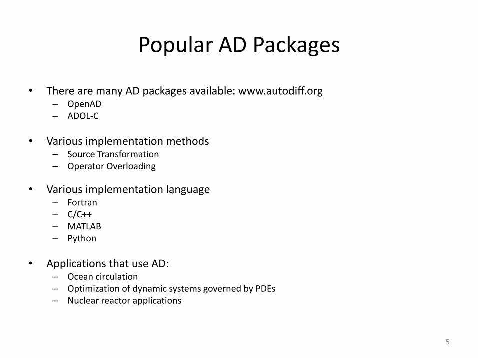
Popular AD Packages

• There are many AD packages available: www.autodiff.org– OpenAD– ADOL-C

• Various implementation methods– Source Transformation– Operator Overloading

• Various implementation language– Fortran– C/C++– MATLAB– Python

• Applications that use AD:– Ocean circulation– Optimization of dynamic systems governed by PDEs– Nuclear reactor applications

5

Challenges for AD in Reservoir Simulation

1. Variable sparsity pattern

6

Diagonal StencilingBlock diagonal

Evaluation

Challenges for AD in Reservoir Simulation

2. Variable switching

7

Automatically Differentiable Expression Templates Library (ADETL)

• Developed by Rami Younis at Stanford University

• Initial prototype to prove viability of AD for reservoir simulation

• ADETL solves some reservoir simulation chanllenges:

– Block sparse gradient data structure

– Two algorithms to compute derivative operations

– Variable switching and adaptive implicit problems

– Builds runtime expression for derivatives

8

Sparse Algorithms in ADETL

9

Algorithm 1: axpy

Phase 1 Phase 2

Sparse Algorithms in ADETL

10

Algorithm 2: running pointers

Variable Switching in ADETL

Independent variable set:

[ Po, Pg, Pw, So, Sg, x1, x2, x3, x4, y1, y2, y3, y4]

Gas phase disappears:

[ Po, Pg, Pw, So, Sg, x1, x2, x3, x4, y1, y2, y3, y4]

11

Components in liquid phase

Components in gas phase

Auto (de)activation

Application of ADETL

• ADETL has been successfully applied in thedevelopment of reservoir simulators:– AD-GPRS (Stanford University)

– Unconventional shale gas reservoir simulator (FuRSST)

• We are improving ADETL towards ADETL 2.0

12

So what’s next?

1. Can we deal with various degrees of sparsity patterns?

2. Can we avoid the cost of runtime sparsity detection?

13

Non-zero Call Stack

14

15

1.2 2.3 1.4

0.5 2.8 2.2

1.2 0.5 0 2.3 4.2 0 2.2 0

0.1 0.2 0.3 0.4

1.2 1.5 1.4 1.8

1.3 1.7 1.7 2.2

1.2

0.7

1.9

Univariate

Dense Multivariate

Sparse Multivariate

ADETL

Stage 1 Univariate terms

Test case: product of sequence

16

𝐹 𝑥 =

𝑖=1

𝑁

𝑓𝑖 𝑥

𝐹′ 𝑥 =

𝑗=1

𝑁𝑑𝑓𝑗 𝑥

𝑑𝑥

𝑖≠𝑗

𝑓𝑖 𝑥

Case # # of arguments (N)

1 3

2 6

3 9

Univariate Test 1

1. Hand differentiation

17

N Value & Derivative Expressions

1 𝐹 𝑥 = 𝑓1 𝑥𝐹′ 𝑥 = 𝑓1

′ 𝑥

2 𝐹 𝑥 = 𝑓1 𝑥 ∗ 𝑓2 𝑥𝐹′ 𝑥 = 𝑓1

′ 𝑥 ∗ 𝑓2 𝑥 + 𝑓1 𝑥 ∗ 𝑓2′ 𝑥

3 𝐹 𝑥 = 𝑓1 𝑥 ∗ 𝑓2 𝑥 ∗ 𝑓3 𝑥𝐹′ 𝑥= 𝑓1

′ 𝑥 ∗ 𝑓2 𝑥 ∗ 𝑓3 𝑥 + 𝑓1 𝑥 ∗ 𝑓2′ 𝑥 ∗ 𝑓3 𝑥 + 𝑓1 𝑥

∗ 𝑓2 𝑥 ∗ 𝑓3′ 𝑥

𝐹 𝑥 =

𝑖=1

𝑁

𝑓𝑖 𝑥

𝐹′ 𝑥 =

𝑗=1

𝑁𝑑𝑓𝑗 𝑥

𝑑𝑥

𝑖≠𝑗

𝑓𝑖 𝑥

Univariate Test 2

2. ADunivariate (new datatype)

18

N ADunivariate Expression

1 R = a

2 R = a * b

3 R = a * b * c

Univariate Test 3

3. ADETL

(block sparse gradient)

19

N ADETL Expression

1 R = a

2 R = a * b

3 R = a * b * c

Univariate Test Result

20

𝐹 𝑥 =

𝑖=1

𝑁

𝑓𝑖 𝑥

𝐹′ 𝑥 =

𝑗=1

𝑁𝑑𝑓𝑗 𝑥

𝑑𝑥

𝑖≠𝑗

𝑓𝑖 𝑥

Stage 2 Dense Multivariate

Test case: summation

21

𝐹 𝑥1, 𝑥2…𝑥𝑛 =

𝑖=1

4

𝑓𝑖 𝑥1, 𝑥2…𝑥𝑛

𝜕𝐹 𝑥1, 𝑥2…𝑥𝑛𝜕𝑥1

=

𝑖=1

4𝜕𝑓𝑖 𝑥1, 𝑥2…𝑥𝑛

𝜕𝑥1

…………

𝜕𝐹 𝑥1, 𝑥2…𝑥𝑛𝜕𝑥𝑛

=

𝑖=1

4𝜕𝑓𝑖 𝑥1, 𝑥2…𝑥𝑛

𝜕𝑥𝑛

Case # # of independent variables

1 5

2 20

3 80

Dense Multivariate Test 1

1. Manual implementation

22

1 2 3 4 5

1 2 3 4 5 … … 20

1 2 3 4 5 … … … … … 79 80

Case 1

Case 2

Case 3

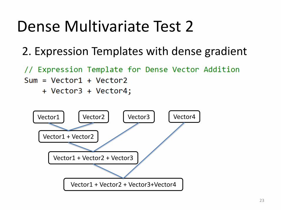
Dense Multivariate Test 2

23

Vector1 Vector2 Vector3

Vector1 + Vector2

Vector1 + Vector2 + Vector3

2. Expression Templates with dense gradient

Vector4

Vector1 + Vector2 + Vector3+Vector4

Dense Multivariate Test 3

3. ADETL (block sparse gradient)

24

1 2 3 4 5

1 2 3 4 5 … … 20

1 2 3 4 5 … … … … … 79 80

Case 1

Case 2

Case 3

Problem 2 - Dense Multivariate

25

𝐹 𝑥1, 𝑥2…𝑥𝑛 =

𝑖=1

𝑁

𝑓𝑖 𝑥1, 𝑥2…𝑥𝑛

0

50000

100000

150000

200000

250000

300000

350000

400000

5 20 80

Tim

e(m

icro

seco

nd

s)

Number of elements in dense vector

Manual Expression Template ADETL

11.4X

4.1X

7.5X

1. Manual2. Expression Template3. ADETL

1X

1X

1X

Avoiding sparse operations

1 2 3 4 5 6 7 8 9 d1 d2 d3 1 2 3

1 x x 1 x x

2 x x x 1 x x x

3 x x x 1 x x x

4 x x x 1 x x x

5 x x x 1 x x x

6 x x x 1 x x x

7 x x x 1 x x x

8 x x x 1 x x x

9 x x 1 x x

x =

26

sparse

Sparse Jacobian Seed matrix Compressed Jacobian

dense

Compressed AD

1. Variable activation

2. Evaluation

27

1

1

1

1

1

1

1

1

1

1 1

2 1

3 1

4 1

5 1

6 1

7 1

8 1

9 1

x x

x x x

x x x

x x x

x x x

x x x

x x x

x x x

x x

x x

x x x

x x x

x x x

x x x

x x x

x x x

x x x

x x

recover

(Dense Jacobian)

𝑱 =

𝑼 =

𝑼 𝑺

𝑱 =

Challenge with Compressed AD

1 2 3 4 5 6 7 8 9 d1 d2 d3 1 2 3

1 x x 1 x x

2 x x x 1 x x x

3 x x x 1 x x x

4 x x x 1 x x x

5 x x x 1 x x x

6 x x x 1 x x x

7 x x x 1 x x x

8 x x x 1 x x x

9 x x 1 x x

x =

28

1. Sparsity pattern is unknown2. Variable switching

Sparse Jacobian Seed matrix Compressed Jacobian

ADETL 2.0

• Full range of data types and efficient algorithms

• Ability to convert from one type to the other

• Compressed AD

• Automatic variable set

• Seed matrix will be incorporated

• Benchmark kernel to test AD packages for reservoir simulation calculations

29

Automatic Differentiation Algorithms and Data Structures

Chen FangPhD Candidate

Joined: January 2013FuRSST Inaugural Annual Meeting

May 8th, 2014

30