automatic differentiation through the use of hyper-dual...
TRANSCRIPT
Automatic Differentiation through the use ofHyper-Dual Numbers for Second Derivatives
Jeffrey A. Fike and Juan J. AlonsoDepartment of Aeronautics and Astronautics, Stanford University, Stanford, CA 94305, U.S.A.
6th International Conference on Automatic DifferentiationFort Collins, CO
July 23, 2012
Outline 2/35
Introduction
First-Derivative Calculations
Second-Derivative CalculationsDiscussion of Desired PropertiesHyper-Dual Numbers
Hyper-Dual Number ImplementationComputational Fluid Dynamics ResultsComputational CostVariations and Extensions
Conclusions
Outline
Introduction
First-Derivative Calculations
Second-Derivative CalculationsDiscussion of Desired PropertiesHyper-Dual Numbers
Hyper-Dual Number ImplementationComputational Fluid Dynamics ResultsComputational CostVariations and Extensions
Conclusions

Introduction 4/35
Automatic Differentiation techniques produce derivatives thatare exact and free from truncation error.
Two approaches for derivation of Automatic Differentiationtechniques:
• Chain rule of differentiation• Forward and Reverse modes• Operator overloading or source transformation
• Use number systems whose mathematics inherentlyproduce the desired derivative information
• Forward mode and operator overloading
Generalized Complex Numbers 5/35
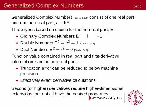
Generalized Complex Numbers [Kantor 1989] consist of one real partand one non-real part, a + bE
Three types based on choice for the non-real part, E :
• Ordinary Complex Numbers E2 = i2 = −1
• Double Numbers E2 = e2 = 1 [Clifford 1873]
• Dual Numbers E2 = ǫ2 = 0 [Study 1903]
Function value contained in real part and first-derivativeinformation is in the non-real part
• Truncation error can be reduced to below machineprecision
• Effectively exact derivative calculations
Second (or higher) derivatives require higher-dimensionalextensions, but not all have the desired properties.

Connection to Automatic Differentiation 6/35
Several authors have made the connection between certainGeneralized Complex Numbers and Automatic Differentiation.
• Ordinary Complex Numbers, i.e. the Complex-StepDerivative Approximation [Martins 2001]
• Dual Numbers [Piponi 2004 and Leuck 1999]
The implementation and use of Dual Numbers is very similar toforward mode approaches that use operator overloading.
• the Doublet class in Evaluating Derivatives [Griewank 2000]
• the tapeless forward mode in ADOL-C

Outline
Introduction
First-Derivative Calculations
Second-Derivative CalculationsDiscussion of Desired PropertiesHyper-Dual Numbers
Hyper-Dual Number ImplementationComputational Fluid Dynamics ResultsComputational CostVariations and Extensions
Conclusions

First-Derivative Calculations 8/35
Generalized Complex Numbers, a + bE , can be used tocompute derivatives of a real-valued function, by evaluating itsubject to a non-real step.
Consider the Taylor Series for a real-valued function with ageneralized complex step,
f (x + hE) = f (x) + hf ′(x)E +12!
h2f ′′(x)E2 +h3f ′′′(x)
3!E3 + ...
• Ordinary Complex Numbers E2 = i2 = −1
• Double Numbers E2 = e2 = 1
• Dual Numbers E2 = ǫ2 = 0
Complex-Step Approximation 9/35
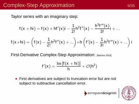
Taylor series with an imaginary step:
f (x + hi) = f (x) + hf ′(x)i − 12!
h2f ′′(x) − h3f ′′′(x)
3!i + ...
f (x+hi) =
(
f (x) − 12!
h2f ′′(x) + ...
)
+h(
f ′(x) − 13!
h2f ′′′(x) + ...
)
i
First-Derivative Complex-Step Approximation: [Martins 2003]
f ′(x) =Im [f (x + hi)]
h+ O(h2)
• First derivatives are subject to truncation error but are notsubject to subtractive cancellation error.

Generalized Complex Numbers 10/35
Ordinary Complex Numbers (E2 = i2 = −1):
f (x+hi) =
(
f (x) − 12!
h2f ′′(x) + ...
)
+h(
f ′(x) − 13!
h2f ′′′(x) + ...
)
i
Double Numbers (E2 = e2 = 1):
f (x+he) =
(
f (x) +12!
h2f ′′(x) + ...
)
+h(
f ′(x) +13!
h2f ′′′(x) + ...
)
e
Dual Numbers (E2 = ǫ2 = 0):
f (x + hǫ) = f (x) + hf ′(x)ǫ

Accuracy of First-Derivative Calculations 11/35
10−30
10−20
10−10
100
10−20
10−15
10−10
10−5
100
Step Size, h
Err
or
Error in the First Derivative
Complex−StepForward−DifferenceCentral−DifferenceHyper−Dual Numbers
f (x) =ex
√
sin3 x + cos3 x

Outline
Introduction
First-Derivative Calculations
Second-Derivative CalculationsDiscussion of Desired PropertiesHyper-Dual Numbers
Hyper-Dual Number ImplementationComputational Fluid Dynamics ResultsComputational CostVariations and Extensions
Conclusions

Generalized Complex Numbers 13/35
Ordinary Complex Numbers (E2 = i2 = −1):
f (x+hi) =
(
f (x) − 12!
h2f ′′(x) + ...
)
+h(
f ′(x) − 13!
h2f ′′′(x) + ...
)
i
Double Numbers (E2 = e2 = 1):
f (x+he) =
(
f (x) +12!
h2f ′′(x) + ...
)
+h(
f ′(x) +13!
h2f ′′′(x) + ...
)
e
Dual Numbers (E2 = ǫ2 = 0):
f (x + hǫ) = f (x) + hf ′(x)ǫ

Second-Derivative Complex-Step 14/35
One Second-Derivative Complex-Step Approximation:
f ′′(x) =2 (f (x) − Re[f (x + ih)])
h2 + O(h2)
• Second derivatives are subject to subtractive cancellation error
Alternative approximations: [Lai 2008]
f ′′(x) =Im[
f (x + i1/2h) + f (x + i5/2h)]
h2 + O(h4)
f ′′(x) =2 Im
[
f (x + i2/3h) + f (x + i8/3h)]
√3h2
+ O(h2)
• These alternatives may offer improvements, but they are stillsubject to subtractive cancellation error
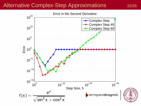
Alternative Complex-Step Approximations 15/35
10−30
10−20
10−10
100
10−15
10−10
10−5
100
105
1010
1015
Step Size, h
Err
or
Error in the Second Derivative
Complex StepComplex Step 45Complex Step 60
f (x) =ex
√
sin3 x + cos3 x

Multiple Non-Real Parts 16/35
To avoid subtractive cancellation error:
• Second-derivative term should be the leading term of anon-real part
• First-derivative is already the leading term of a non-realpart
Suggests that we need a number with multiple non-real parts
• Use higher-dimensional extensions of generalized complexnumbers

Quaternions 17/35
Quaternions: one real part and three non-real parts
i2 = j2 = k2 = −1
ijk = −1
Taylor series for a generic step, d :
f (x + d) = f (x) + df ′(x) +12!
d2f ′′(x) +13!
d3f ′′′(x) + ...
For a quaternion step:
d = h1i + h2j + 0k
d2 = −(
h21 + h2
2
)
• d2 is real, second derivative only appears in the real part

Quaternions 18/35
Second-Derivative Quaternion-Step Approximation:
f ′′(x) =2 (f (x) − Re[f (x + h1i + h2j + 0k)])
h21 + h2
2
+ O(h21 + h2
2)
• Subject to subtractive-cancellation error
Quaternion multiplication is not commutative, ij = k but ji = −k
Instead, consider a number with three non-real components E1,E2, and (E1E2) where multiplication is commutative, i.e.E1E2 = E2E1
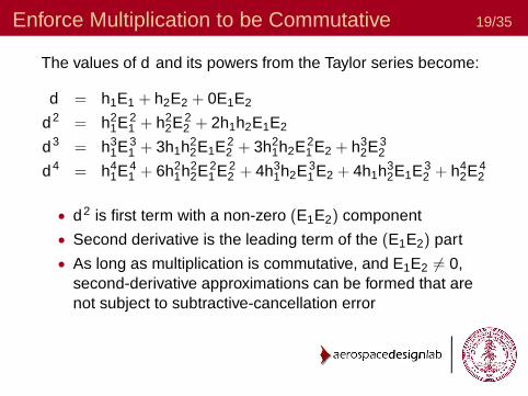
Enforce Multiplication to be Commutative 19/35
The values of d and its powers from the Taylor series become:
d = h1E1 + h2E2 + 0E1E2
d2 = h21E2
1 + h22E2
2 + 2h1h2E1E2
d3 = h31E3
1 + 3h1h22E1E2
2 + 3h21h2E2
1 E2 + h32E3
2
d4 = h41E4
1 + 6h21h2
2E21 E2
2 + 4h31h2E3
1 E2 + 4h1h32E1E3
2 + h42E4
2
• d2 is first term with a non-zero (E1E2) component
• Second derivative is the leading term of the (E1E2) part
• As long as multiplication is commutative, and E1E2 6= 0,second-derivative approximations can be formed that arenot subject to subtractive-cancellation error

Several Possible Number Systems 20/35
The requirement that E1E2 = E2E1 produces the constraint:
(E1E2)2 = E1E2E1E2 = E1E1E2E2 = E2
1 E22
This leaves many possibilities for the definitions of E1 and E2:• E2
1 = E22 = −1 which results in (E1E2)
2 = 1• Circular-Fourcomplex Numbers [Olariu 2002]
• Multicomplex Numbers [Price 1991]
• Constrain E21 = E2
2 = (E1E2)2
• E21 = E2
2 = (E1E2)2 = 1 Hyper-Double Numbers
• E21 = E2
2 = (E1E2)2 = 0 Hyper-Dual Numbers [Fike 2011]
All are free from subtractive-cancellation error
• Truncation error can be reduced below machine precision
• Effectively exact

Hyper-Dual Numbers 21/35
Hyper-dual numbers have one real part and three non-realparts:
a = a0 + a1ǫ1 + a2ǫ2 + a3ǫ1ǫ2
ǫ21 = ǫ2
2 = 0
ǫ1 6= ǫ2 6= 0
ǫ1ǫ2 = ǫ2ǫ1 6= 0
Taylor series truncates exactly at second-derivative term:
f (x+h1ǫ1+h2ǫ2+0ǫ1ǫ2) = f (x)+h1f ′(x)ǫ1+h2f ′(x)ǫ2+h1h2f ′′(x)ǫ1ǫ2
• No truncation error and no subtractive-cancellation error
Fike and Alonso, AIAA 2011-886

Accuracy of Second-Derivative Calculations 22/35
10−30
10−20
10−10
100
10−20
10−10
100
1010
1020
Step Size, h
Err
or
Error in the Second Derivative
Complex−StepForward−DifferenceCentral−DifferenceHyper−Dual Numbers
f (x) =ex
√
sin3 x + cos3 x

Outline
Introduction
First-Derivative Calculations
Second-Derivative CalculationsDiscussion of Desired PropertiesHyper-Dual Numbers
Hyper-Dual Number ImplementationComputational Fluid Dynamics ResultsComputational CostVariations and Extensions
Conclusions

Hyper-Dual Numbers 24/35
Evaluate a function with a hyper-dual step:
f (x + h1ǫ1ei + h2ǫ2ej + 0ǫ1ǫ2)
Derivative information can be found by examining the non-realparts:
∂f (x)
∂xi=
ǫ1part[
f (x + h1ǫ1ei + h2ǫ2ej + 0ǫ1ǫ2)]
h1
∂f (x)
∂xj=
ǫ2part[
f (x + h1ǫ1ei + h2ǫ2ej + 0ǫ1ǫ2)]
h2
∂2f (x)
∂xi∂xj=
ǫ1ǫ2part[
f (x + h1ǫ1ei + h2ǫ2ej + 0ǫ1ǫ2)]
h1h2

Hyper-Dual Number Implementation 25/35
To use hyper-dual numbers, every operation in an analysiscode must be modified to operate on hyper-dual numbersinstead of real numbers
• Basic Arithmetic Operations: Addition, Multiplication, etc.
• Logical Comparison Operators: ≥, 6=, etc.
• Mathematical Functions: exponential, logarithm, sine, absolutevalue, etc.
• Input/Output Functions to write and display hyper-dual numbers
Hyper-dual numbers are implemented as a class usingoperator overloading in C++, CUDA and MATLAB
• Change variable types
• Body and structure of code unaltered
Implementation available from http://adl.stanford.edu/MPI datatype and reduction operations also available

Computational Fluid Dynamics Code 26/35
Joe [Pecnik 2009]
• Parallel, unstructured, 3-D, multi-physics, unsteadyReynolds-Averaged Navier-Stokes code
• Developed at Stanford under the sponsorship of theDepartment of Energy under the Predictive ScienceAcademic Alliance Program
• Written in C++, which enables straightforward conversionto hyper-dual numbers
To demonstrate the accuracy of the hyper-dual numbercalculations, the derivative calculations need to be compared toexact values
• Inviscid, supersonic flow over a wedge
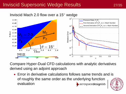
Inviscid Supersonic Wedge Results 27/35
Inviscid Mach 2.0 flow over a 15◦ wedge
M1 = 2.0
P1
M2
P2
βθ = 15◦
0 0.2 0.4 0.6 0.8 110
−8
10−6
10−4
10−2
100
102
x
Rel
ativ
e E
rror
Pressure Ratio, P2/P
1
First Derivative of P2/P
1 w.r.t. Mach Number
Second Derivative of P2/P
1 w.r.t. Mach Number.
Compare Hyper-Dual CFD calculations with analytic derivativesderived using an adjoint approach
• Error in derivative calculations follows same trends and isof roughly the same order as the underlying functionevaluation
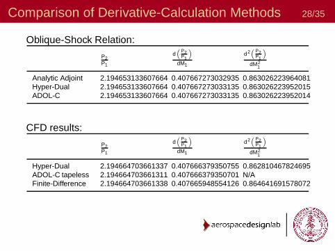
Comparison of Derivative-Calculation Methods 28/35
Oblique-Shock Relation:
P2P1
d“
P2P1
”
dM1
d2“
P2P1
”
dM21
Analytic Adjoint 2.194653133607664 0.407667273032935 0.863026223964081Hyper-Dual 2.194653133607664 0.407667273033135 0.863026223952015ADOL-C 2.194653133607664 0.407667273033135 0.863026223952014
CFD results:
P2P1
d“
P2P1
”
dM1
d2“
P2P1
”
dM21
Hyper-Dual 2.194664703661337 0.407666379350755 0.862810467824695ADOL-C tapeless 2.194664703661311 0.407666379350701 N/AFinite-Difference 2.194664703661338 0.407665948554126 0.864641691578072
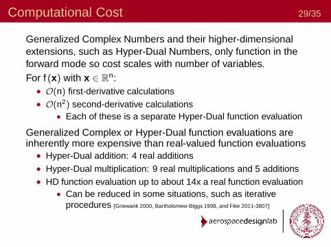
Computational Cost 29/35
Generalized Complex Numbers and their higher-dimensionalextensions, such as Hyper-Dual Numbers, only function in theforward mode so cost scales with number of variables.For f (x) with x ∈ R
n:• O(n) first-derivative calculations• O(n2) second-derivative calculations
• Each of these is a separate Hyper-Dual function evaluation
Generalized Complex or Hyper-Dual function evaluations areinherently more expensive than real-valued function evaluations
• Hyper-Dual addition: 4 real additions• Hyper-Dual multiplication: 9 real multiplications and 5 additions• HD function evaluation up to about 14x a real function evaluation
• Can be reduced in some situations, such as iterativeprocedures [Griewank 2000, Bartholomew-Biggs 1998, and Fike 2011-3807]

Computational Cost 30/35
Each second-derivative calculation using hyper-dual numbersis independent
• Function values and first derivatives are re-computed asrequired
• Limits memory requirements to only 4 times that of the realnumber version
• Can make differentiation more tractable for problems wherememory is often a limiting factor, such as large CFDcalculations
• Communication for parallel function evaluations using MPIalso only increases by a factor of 4

Available Variations 31/35
Implementations are available for a few variations• Vectorized version
• When computing the Hessian, the standard Hyper-Dualimplementation results in redundant function andfirst-derivative calculations
• Vectorized version propagates entire gradient and Hessian• Eliminates redundant calculations, but increased
memory requirements
• Derivatives of complex-valued functions• Hyper-Dual numbers with complex-valued components

Higher-Order Derivatives 32/35
Methods for computing higher derivatives can be created byusing more non-real parts
Include ǫ3 terms and look at powers of d from the Taylor series:
d = h1ǫ1 + h2ǫ2 + h3ǫ3 + 0ǫ1ǫ2 + 0ǫ1ǫ3 + 0ǫ2ǫ3 + 0ǫ1ǫ2ǫ3
d2 = 2h1h2ǫ1ǫ2 + 2h1h3ǫ1ǫ3 + 2h2h3ǫ2ǫ3
d3 = 6h1h2h3ǫ1ǫ2ǫ3
d4 = 0
• d3 is first term with a non-zero ǫ1ǫ2ǫ3 component
• Third derivative is the leading term of the ǫ1ǫ2ǫ3 part, sothird derivative calculations are free from subtractivecancellation error
• d4 and higher powers of d are zero, so there is notruncation error

Outline
Introduction
First-Derivative Calculations
Second-Derivative CalculationsDiscussion of Desired PropertiesHyper-Dual Numbers
Hyper-Dual Number ImplementationComputational Fluid Dynamics ResultsComputational CostVariations and Extensions
Conclusions
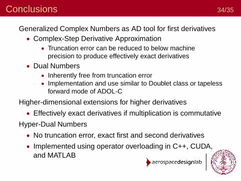
Conclusions 34/35
Generalized Complex Numbers as AD tool for first derivatives• Complex-Step Derivative Approximation
• Truncation error can be reduced to below machineprecision to produce effectively exact derivatives
• Dual Numbers• Inherently free from truncation error• Implementation and use similar to Doublet class or tapeless
forward mode of ADOL-C
Higher-dimensional extensions for higher derivatives
• Effectively exact derivatives if multiplication is commutative
Hyper-Dual Numbers
• No truncation error, exact first and second derivatives
• Implemented using operator overloading in C++, CUDA,and MATLAB

Questions?

Backup Slides

Finite Difference Formulas 37/35
Forward-difference (FD) Approximation:
∂f (x)
∂xj=
f (x + hej) − f (x)
h+ O(h)
Central-Difference (CD) approximation:
∂f (x)
∂xj=
f (x + hej) − f (x − hej)
2h+ O(h2)
Subject to truncation error and subtractive cancellation error• Truncation error is associated with the higher order terms that
are ignored when forming the approximation.
• Subtractive cancellation error is a result of performing thesecalculations on a computer with finite precision.
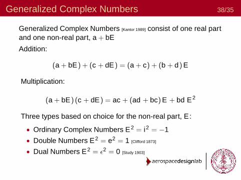
Generalized Complex Numbers 38/35
Generalized Complex Numbers [Kantor 1989] consist of one real partand one non-real part, a + bE
Addition:
(a + bE) + (c + dE) = (a + c) + (b + d) E
Multiplication:
(a + bE) (c + dE) = ac + (ad + bc) E + bd E2
Three types based on choice for the non-real part, E :
• Ordinary Complex Numbers E2 = i2 = −1
• Double Numbers E2 = e2 = 1 [Clifford 1873]
• Dual Numbers E2 = ǫ2 = 0 [Study 1903]

Extension of Dual Numbers 39/35
Complex Numbers:
a + bi
i2 = −1
Quaternions:
a + bi + cj + dk
i2 = j2 = k2 = −1
ij = −ji = k
Dual Numbers:
a + bǫ
ǫ2 = 0, ǫ 6= 0
Hyper-Dual Numbers:
a + bǫ1 + cǫ2 + dǫ1ǫ2
ǫ21 = ǫ2
2 = (ǫ1ǫ2)2 = 0
ǫ1 6= ǫ2 6= ǫ1ǫ2 6= 0

Arithmetic Operations 40/35
Consider two Hyper-Dual Numbers:
a = a0 + a1ǫ1 + a2ǫ2 + a3ǫ1ǫ2 b = b0 + b1ǫ1 + b2ǫ2 + b3ǫ1ǫ2
Addition:
a + b = (a0 + b0) + (a1 + b1) ǫ1 + (a2 + b2) ǫ2 + (a3 + b3) ǫ1ǫ2
Multiplication:
a ∗ b = (a0 ∗ b0) + (a0 ∗ b1 + a1 ∗ b0) ǫ1 + (a0 ∗ b2 + a2 ∗ b0) ǫ2
+ (a0 ∗ b3 + a1 ∗ b2 + a2 ∗ b1 + a3 ∗ b0) ǫ1ǫ2

Other Operations 41/35
The inverse:
1a
=1a0
− a1
a20
ǫ1 −a2
a20
ǫ2 −(
2a1a2
a30
− a3
a20
)
ǫ1ǫ2
• Only exists for a0 6= 0
This suggests a definition for the norm:
norm (a) =√
a20
This in turn implies that comparisons should only be madebased on the real part.
• i.e. a > b is equivalent to a0 > b0
• This allows the code to follow the same execution path asthe real-valued code.
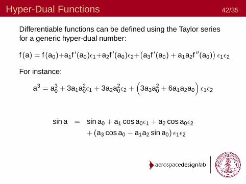
Hyper-Dual Functions 42/35
Differentiable functions can be defined using the Taylor seriesfor a generic hyper-dual number:
f (a) = f (a0)+a1f ′(a0)ǫ1+a2f ′(a0)ǫ2+(
a3f ′(a0) + a1a2f ′′(a0))
ǫ1ǫ2
For instance:
a3 = a30 + 3a1a2
0ǫ1 + 3a2a20ǫ2 +
(
3a3a20 + 6a1a2a0
)
ǫ1ǫ2
sin a = sin a0 + a1 cos a0ǫ1 + a2 cos a0ǫ2
+ (a3 cos a0 − a1a2 sin a0) ǫ1ǫ2

Other Functions 43/35
Non-differentiable functions, such as the absolute value, can bedefined as a procedureif x<0 return -x else return xThis ignores any issues at the discontinuity.

Simple Example 44/35
f (x) = sin3 x
This function can be evaluated as:
t0 = x
t1 = sin t0t2 = t3
1

Hyper-Dual Evaluation 45/35
t0 = x + h1ǫ1 + h2ǫ2 + 0ǫ1ǫ2
t1 = sin t0= sin x + h1 cos xǫ1 + h2 cos xǫ2 − h1h2 sin xǫ1ǫ2
t2 = t31
= sin3 x + 3h1 cos x sin2 xǫ1 + 3h2 cos x sin2 xǫ2
−34
h1h2 (sin x − 3 sin 3x) ǫ1ǫ2

Division Algebra 46/35
Real numbers, ordinary complex numbers and quaternions aredivision algebras.
• Additive associativity, additive commutativity, additiveidentity, additive inverse, multiplicative associativity,multiplicative identity, multiplicative inverse, left and rightdistributivity
Hyper-Dual Numbers satisfy all these conditions except for themultiplicative inverse.
• Requirement: an inverse exists for all numbers not equal tozero
• Hyper-Dual Numbers: an inverse exists for all numberswhose norm is not equal to zero
• i.e. if the real part is not equal to zero

Supersonic Wedge 47/35
Inviscid Mach 2.0 flow over a 15◦ wedgeCompute derivatives of the pressure ratio, P2
P1, across the
resulting oblique shock with respect to the incoming MachnumberPressure ratio across an oblique shock:
Pratio =P2
P1= 1 +
2γ
γ + 1
(
M21 sin2 β − 1
)
Analytic derivatives can be derived using an adjoint approachby casting the oblique-shock relation as a residual equation:
R =2 cot β
(
M21 sin2 β − 1
)
M21 (γ + cos 2β) + 2
− tan θ = 0
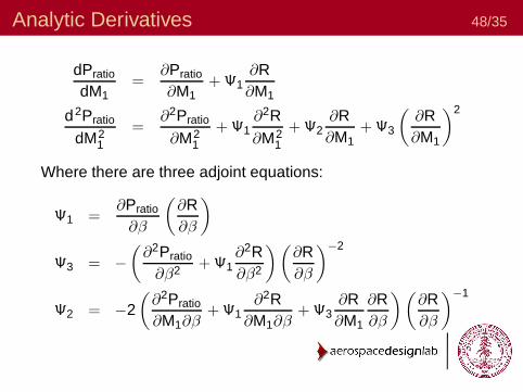
Analytic Derivatives 48/35
dPratio
dM1=
∂Pratio
∂M1+ Ψ1
∂R∂M1
d2Pratio
dM21
=∂2Pratio
∂M21
+ Ψ1∂2R∂M2
1
+ Ψ2∂R∂M1
+ Ψ3
(
∂R∂M1
)2
Where there are three adjoint equations:
Ψ1 =∂Pratio
∂β
(
∂R∂β
)
Ψ3 = −(
∂2Pratio
∂β2 + Ψ1∂2R∂β2
)(
∂R∂β
)
−2
Ψ2 = −2(
∂2Pratio
∂M1∂β+ Ψ1
∂2R∂M1∂β
+ Ψ3∂R∂M1
∂R∂β
)(
∂R∂β
)
−1
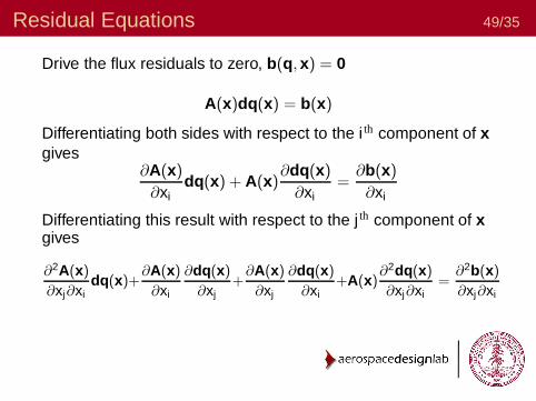
Residual Equations 49/35
Drive the flux residuals to zero, b(q, x) = 0
A(x)dq(x) = b(x)
Differentiating both sides with respect to the i th component of xgives
∂A(x)
∂xidq(x) + A(x)
∂dq(x)
∂xi=
∂b(x)
∂xi
Differentiating this result with respect to the j th component of xgives
∂2A(x)
∂xj∂xidq(x)+
∂A(x)
∂xi
∂dq(x)
∂xj+
∂A(x)
∂xj
∂dq(x)
∂xi+A(x)
∂2dq(x)
∂xj∂xi=
∂2b(x)
∂xj∂xi

Residual Equations 50/35
This can be solved as:
A(x) 0 0 0∂A(x)
∂xiA(x) 0 0
∂A(x)∂xj
0 A(x) 0∂
2A(x)∂xj ∂xi
∂A(x)∂xj
∂A(x)∂xi
A(x)
dq(x)∂dq(x)
∂xi∂dq(x)
∂xj
∂2dq(x)∂xj ∂xi
=
b(x)∂b(x)∂xi
∂b(x)∂xj
∂2b(x)
∂xj ∂xi
Or A(x)dq(x) = b(x)
A(x)∂dq(x)
∂xi=
∂b(x)
∂xi− ∂A(x)
∂xidq(x)
A(x)∂dq(x)
∂xj=
∂b(x)
∂xj− ∂A(x)
∂xjdq(x)
A(x)∂2dq(x)
∂xj∂xi=
∂2b(x)
∂xj∂xi−∂2A(x)
∂xj∂xidq(x)−∂A(x)
∂xi
∂dq(x)
∂xj−∂A(x)
∂xj
∂dq(x)
∂xi

Start from Converged Solution 51/35
For a converged solution, dq(x) ≡ 0. This simplifies theprocedure to:
A(x)∂dq(x)
∂xi=
∂b(x)
∂xi
A(x)∂dq(x)
∂xj=
∂b(x)
∂xj
A(x)∂2dq(x)
∂xj∂xi=
∂2b(x)
∂xj∂xi− ∂A(x)
∂xi
∂dq(x)
∂xj− ∂A(x)
∂xj
∂dq(x)
∂xi
If we now assume that we have converged the first derivativeterms, then the second-derivative equation reduces to
A(x)∂2dq(x)
∂xj∂xi=
∂2b(x)
∂xj∂xi

Initial Tests 52/35
This approach is applied to the CFD code JOE• Parallel, unstructured, 3-D, multi-physics, unsteady
Reynolds-Averaged Navier-Stokes code
• Written in C++, which enables the straightforward conversion tohyper-dual numbers
• Can use PETSc to solve the linear system
0 2000 4000 6000 8000 10000 12000 14000 16000Iteration
10-16
10-14
10-12
10-10
10-8
10-6
10-4
10-2
100
Resi
dual
NACA 0012, M=0.8, �=1�, inviscid, 1st order.
Convergence of �2 cl/���M.
Density, Cold Start, GMRES2nd Deriv, Cold Start, GMRES2nd Deriv, Restart, Flow Updated, GMRES2nd Deriv, Restart, Flow Frozen, GMRES2nd Deriv, Restart, Flow Frozen, LU
Derivatives converge at samerate as flow solution
• No benefit to starting witha converged solution?
• JOE uses an approximateJacobian
• Need the exact Jacobian
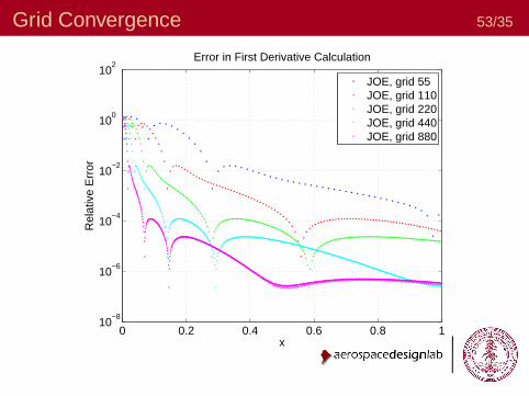
Grid Convergence 53/35
0 0.2 0.4 0.6 0.8 110
−8
10−6
10−4
10−2
100
102
x
Rel
ativ
e E
rror
Error in First Derivative Calculation
JOE, grid 55JOE, grid 110JOE, grid 220JOE, grid 440JOE, grid 880
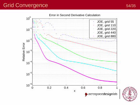
Grid Convergence 54/35
0 0.2 0.4 0.6 0.8 110
−6
10−5
10−4
10−3
10−2
10−1
100
x
Rel
ativ
e E
rror
Error in Second Derivative Calculation
JOE, grid 55JOE, grid 110JOE, grid 220JOE, grid 440JOE, grid 880

Alternative Complex-Step Approximations 55/35
10−30
10−20
10−10
100
10−20
10−15
10−10
10−5
100
Step Size, h
Err
or
Error in the First Derivative
Complex StepComplex Step 45Complex Step 60
f (x) =ex
√
sin3 x + cos3 x

Alternative Complex-Step Approximations 56/35
10−30
10−20
10−10
100
10−15
10−10
10−5
100
105
1010
1015
Step Size, h
Err
or
Error in the Second Derivative
Complex StepComplex Step 45Complex Step 60
f (x) =ex
√
sin3 x + cos3 x

Single-Precision Calculations 57/35
10−50
100
10−8
10−6
10−4
10−2
100
Step Size, h
Err
or
Error in the First Derivative
Complex StepForward DifferenceCentral DifferenceHyper−Dual Numbers
f (x) =ex
√
sin3 x + cos3 x
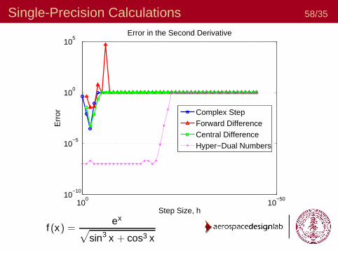
Single-Precision Calculations 58/35
10−50
100
10−10
10−5
100
105
Step Size, h
Err
or
Error in the Second Derivative
Complex StepForward DifferenceCentral DifferenceHyper−Dual Numbers
f (x) =ex
√
sin3 x + cos3 x

Alternative Complex-Step Approximations 59/35
10−50
100
10−8
10−6
10−4
10−2
100
102
Step Size, h
Err
or
Error in the First Derivative
Complex StepComplex Step 45Complex Step 60
f (x) =ex
√
sin3 x + cos3 x
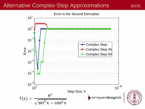
Alternative Complex-Step Approximations 60/35
10−50
100
10−5
10−4
10−3
10−2
10−1
100
101
Step Size, h
Err
or
Error in the Second Derivative
Complex StepComplex Step 45Complex Step 60
f (x) =ex
√
sin3 x + cos3 x
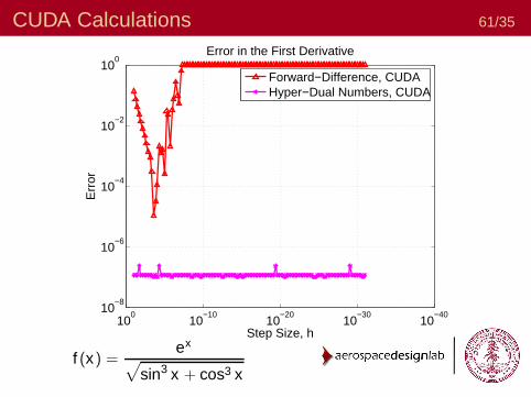
CUDA Calculations 61/35
10−40
10−30
10−20
10−10
100
10−8
10−6
10−4
10−2
100
Step Size, h
Err
or
Error in the First Derivative
Forward−Difference, CUDAHyper−Dual Numbers, CUDA
f (x) =ex
√
sin3 x + cos3 x

CUDA Calculations 62/35
10−40
10−30
10−20
10−10
100
10−10
10−5
100
105
1010
Step Size, h
Err
or
Error in the Second Derivative
Forward−Difference, CUDAHyper−Dual Numbers, CUDA
f (x) =ex
√
sin3 x + cos3 x

CUDA Comparisons 63/35
10−40
10−30
10−20
10−10
100
10−10
10−8
10−6
10−4
10−2
100
Step Size, h
Err
or
Error in the First Derivative
Forward−Difference CPUForward−Difference GPU
f (x) =ex
√
sin3 x + cos3 x

CUDA Comparisons 64/35
10−40
10−30
10−20
10−10
100
10−5
100
105
1010
1015
1020
Step Size, h
Err
or
Error in the Second Derivative
Forward−Difference CPUForward−Difference GPU
f (x) =ex
√
sin3 x + cos3 x