Automatic Differentiation Tutorial

Paul Hovland

Andrew Lyons

Boyana Norris

Jean Utke

Mathematics & Computer Science Division

Argonne National Laboratory

Modes of AD

Forward Mode – Propagates derivative vectors, often denoted u or g_u– Derivative vector u contains derivatives of u with respect to independent variables– Time and storage proportional to vector length (# indeps)

Reverse Mode– Propagates adjoints, denoted ū or u_bar – Adjoint ū contains derivatives of dependent variables with respect to u– Propagation starts with dependent variables—must reverse flow of computation– Time proportional to adjoint vector length (# dependents)– Storage proportional to number of operations – Because of this limitation, often applied to subprograms

Which mode to use?

Use forward mode when

– # independents is very small

– Only a directional derivative (Jv) is needed

– Reverse mode is not tractable Use reverse mode when

– # dependents is very small

– Only JTv is needed

Ways of Implementing AD

Operator Overloading– Use language features to implement differentiation rules or to generate trace

(“tape”) of computation– Implementation can be very simple– Difficult to go beyond one operation/statement at a time in doing AD– Potential overhead due to compiler-generated temporaries,

e.g. w = x*y*z tmp = x*y; w = tmp*z.– Examples: ADOL-C, ADMAT, TFAD<>,SACADO

Source Transformation– Requires significant (compiler) infrastructure– More flexibility in exploiting chain rule associativity– Examples: ADIFOR, ADIC, OpenAD, TAF, TAPENADE

Operator Overloading: simple example (implementation)

class a_double{private: double value, grad;public: /* constructors */ a_double(double v=0.0, double g=0.0){value=v; grad = g;}

/* operators */ friend a_double operator+(const a_double &g1, const a_double &g2) { return a_double(g1.value+g2.value,g1.grad+g2.grad); } friend a_double operator-(const a_double &g1, const a_double &g2) { return a_double(g1.value-g2.value,g1.grad-g2.grad); } friend a_double operator*(const a_double &g1, const a_double &g2) { return a_double(g1.value*g2.value,g2.value*g1.grad+g1.value*g2.grad); } friend a_double sin(const a_double &g1) { return a_double(sin(g1.value),cos(g1.value)*g1.grad); } friend a_double cos(const a_double &g1) { return a_double(cos(g1.value),-sin(g1.value)*g1.grad); } // ...

Operator Overloading: simple example (use)

#include <math.h>#include <stream.h>#include "adouble.hxx"

void func(a_double *f, a_double x, a_double y){ a_double a,b;

if (x > y) { a = cos(x); b = sin(y)*y*y; } else { a = x*sin(x)/y; b = exp(y); } *f = exp(a*b);}

Source Transformation: simple example

C Generated by TAPENADE (INRIA, Tropics team)C ... SUBROUTINE FUNC_D(f, fd, x, xd, y, yd) DOUBLE PRECISION f, fd, x, xd, y, yd DOUBLE PRECISION a, ad, arg1, arg1d, b, bd INTRINSIC COS, EXP, SINC IF (x .GT. y) THEN ad = -(xd*SIN(x)) a = COS(x) bd = yd*COS(y)*y*y + SIN(y)*(yd*y+y*yd) b = SIN(y)*y*y ELSE ad = ((xd*SIN(x)+x*xd*COS(x))*y-x*SIN(x)*yd)/y**2 a = x*SIN(x)/y bd = yd*EXP(y) b = EXP(y) END IF arg1d = ad*b + a*bd arg1 = a*b fd = arg1d*EXP(arg1) f = EXP(arg1) RETURN END

Tools

Fortran 95 C/C++ Fortran 77 MATLAB Other languages: Ada, Python, ... More tools at http://www.autodiff.org/

Tools: Fortran 95

TAF (FastOpt)

– Commercial tool

– Support for (almost) all of Fortran 95

– Used extensively in geophysical sciences applications Tapenade (INRIA)

– Support for many Fortran 95 features

– Developed by a team with extensive compiler experience OpenAD/F (Argonne/UChicago/Rice)

– Support for many Fortran 95 features

– Developed by a team with expertise in combintorial algorithms, compilers, software engineering, and numerical analysis

– Development driven by climate model & astrophysics code All three: forward and reverse; source transformation

Tools: C/C++

ADOL-C (Dresden)– Mature tool– Support for all of C++– Operator overloading; forward and reverse modes

ADIC (Argonne/UChicago)– Support for all of C, some C++– Source transformation; forward mode (reverse under development)– New version (2.0) based on industrial strength compiler infrastructure– Shares some infrastructure with OpenAD/F

SACADO: – Operator overloading; forward and reverse modes– See Phipps presentation

TAC++ (FastOpt)– Commercial tool (under development)– Support for much of C/C++– Source transformation; forward and reverse modes– Shares some infrastructure with TAF

Tools: Fortran 77

ADIFOR (Rice/Argonne)

– Mature and very robust tool

– Support for all of Fortran 77

– Forward and (adequate) reverse modes

– Hundreds of users; ~150 citations

AdiMat (Aachen): source transformation MAD (Cranfield/TOMLAB): operator overloading Various research prototypes

Tools: MATLAB

ADIFOR 2.0: simple example (x only)

C This file was generated on 09/15/03 by the version ofC ADIFOR compiled on June, 1998.C ... subroutine g_func(f, g_f, x, g_x, y) double precision f, x, y, a, b double precision d1_w, d2_v, d1_p, d2_b, g_a, g_x, g_d1_w, g_f save g_a, g_d1_w

if (x .gt. y) then d2_v = cos(x) d1_p = -sin(x) g_a = d1_p * g_x a = d2_vC-------- b = sin(y) * y * y else d2_v = sin(x) d1_p = cos(x) d2_b = 1.0d0 / y g_a = (d2_b * d2_v + d2_b * x * d1_p) * g_x a = x * d2_v / yC-------- b = exp(y) endif g_d1_w = b * g_a d1_w = a * b d2_v = exp(d1_w) d1_p = d2_v g_f = d1_p * g_d1_w f = d2_vC--------C return end

ADIFOR 3.0: simple example subroutine g_func_proc(ad_p_, f, g_f, x, g_x, y, g_y) include 'g_maxs.h'c+declarations here integer ad_p_ double precision d_tmp_s_0_a double precision g_a(ad_pmax_) double precision g_b(ad_pmax_) double precision g_f(ad_pmax_) double precision g_X2_dtmp1(ad_pmax_) double precision g_x(ad_pmax_) double precision g_y(ad_pmax_) double precision d_tmp_ipar_0 double precision d_tmp_val_0 double precision d_tmp_val_1 double precision f, x, y, a, b double precision X2_dtmp1C+AD4 Start of executable statements. d_tmp_ipar_0 = (-sin(x)) call g_accum_d_2(ad_p_, g_a, d_tmp_ipar_0, g_x) a = cos(x) d_tmp_val_0 = sin(y) d_tmp_val_1 = d_tmp_val_0 * y d_tmp_ipar_0 = cos(y) d_tmp_s_0_a = d_tmp_val_1 + y * d_tmp_val_0 + y * y * d_tmp_ipar +_0 call g_accum_d_2(ad_p_, g_b, d_tmp_s_0_a, g_y) b = d_tmp_val_1 * y call g_accum_d_4(ad_p_, g_X2_dtmp1, a, g_b, b, g_a) X2_dtmp1 = a * b d_tmp_ipar_0 = exp(X2_dtmp1) call g_accum_d_2(ad_p_, g_f, d_tmp_ipar_0, g_X2_dtmp1) f = exp(X2_dtmp1)C return end

TAPENADE reverse mode: simple example

C Generated by TAPENADE (INRIA, Tropics team)C Version 2.0.6 - (Id: 1.14 vmp Stable - Fri Sep 5 14:08:23 MEST 2003)C ... SUBROUTINE FUNC_B(f, fb, x, xb, y, yb) DOUBLE PRECISION f, fb, x, xb, y, yb DOUBLE PRECISION a, ab, arg1, arg1b, b, bb INTEGER branch INTRINSIC COS, EXP, SINC IF (x .GT. y) THEN a = COS(x) b = SIN(y)*y*y CALL PUSHINTEGER4(0) ELSE a = x*SIN(x)/y b = EXP(y) CALL PUSHINTEGER4(1) END IF arg1 = a*b f = EXP(arg1) arg1b = EXP(arg1)*fb ab = b*arg1b bb = a*arg1b CALL POPINTEGER4(branch) IF (branch .LT. 1) THEN yb = yb + (SIN(y)*y+y*SIN(y)+y*y*COS(y))*bb xb = xb - SIN(x)*ab ELSE yb = yb + EXP(y)*bb - x*SIN(x)*ab/y**2 xb = xb + (x*COS(x)/y+SIN(x)/y)*ab END IF fb = 0.D0 END

OpenAD system architecture

OpenAD: simple example

SUBROUTINE func(F, X, Y) use w2f__types use active_moduleC Declarations C ... IF (X%v .GT. Y%v) THEN OpenAD_Symbol_1 = COS(X%v) OpenAD_Symbol_0 = (-SIN(X%v)) A%v = OpenAD_Symbol_1 OpenAD_Symbol_5 = SIN(Y%v) OpenAD_Symbol_2 = (Y%v*OpenAD_Symbol_5) OpenAD_Symbol_9 = (Y%v*OpenAD_Symbol_2) OpenAD_Symbol_3 = OpenAD_Symbol_2 OpenAD_Symbol_6 = OpenAD_Symbol_5 OpenAD_Symbol_8 = COS(Y%v) OpenAD_Symbol_7 = Y%v OpenAD_Symbol_4 = Y%v B%v = OpenAD_Symbol_9 OpenAD_Symbol_25 = (OpenAD_Symbol_6 + OpenAD_Symbol_8 * > OpenAD_Symbol_7) OpenAD_Symbol_26 = (OpenAD_Symbol_3 + OpenAD_Symbol_25 * > OpenAD_Symbol_4) OpenAD_Symbol_28 = OpenAD_Symbol_0 CALL setderiv(OpenAD_Symbol_29,X) CALL setderiv(OpenAD_Symbol_27,Y) CALL sax(OpenAD_Symbol_26,OpenAD_Symbol_27,B) CALL sax(OpenAD_Symbol_28,OpenAD_Symbol_29,A) ELSEC ...

ADIC: simple example

#include "ad_deriv.h"#include <math.h>#include "adintrinsics.h"void ad_func(DERIV_TYPE *f,DERIV_TYPE x,DERIV_TYPE y) {DERIV_TYPE a, b, ad_var_0, ad_var_1, ad_var_2;double ad_adji_0,ad_loc_0,ad_loc_1,ad_adj_0,ad_adj_1,ad_adj_2,ad_adj_3;

if (DERIV_val(x) > DERIV_val(y)) { DERIV_val(a) = cos( DERIV_val(x)); /*cos*/ ad_adji_0 = -sin( DERIV_val(x)); { ad_grad_axpy_1(&(a), ad_adji_0, &(x)); } DERIV_val(ad_var_0) = sin( DERIV_val(y)); /*sin*/ ad_adji_0 = cos( DERIV_val(y)); { ad_grad_axpy_1(&(ad_var_0), ad_adji_0, &(y)); } { ad_loc_0 = DERIV_val(ad_var_0) * DERIV_val(y); ad_loc_1 = ad_loc_0 * DERIV_val(y); ad_adj_0 = DERIV_val(ad_var_0) * DERIV_val(y); ad_adj_1 = DERIV_val(y) * DERIV_val(y); ad_grad_axpy_3(&(b), ad_adj_1, &(ad_var_0), ad_adj_0, &(y), ad_loc_0, &(y)); DERIV_val(b) = ad_loc_1; } } else { // ...

ADIC-Generated Code: Interpretation

DERIV_val(y): value of program variable y

DERIV_grad(y):derivative object associated with y

Original code: y = x1*x2*x3*x4;typedef struct { double value; double grad[ad_GRAD_MAX];} DERIV_TYPE;

ad_loc_0 = DERIV_val(x1) * DERIV_val(x2);ad_loc_1 = ad_loc_0 * DERIV_val(x3); dy/dx4ad_loc_2 = ad_loc_1 * DERIV_val(x4); yad_adj_0 = ad_loc_0 * DERIV_val(x4); dy/dx3ad_adj_1 = DERIV_val(x3) * DERIV_val(x4);ad_adj_2 = DERIV_val(x1) * ad_adj_1; dy/dx2ad_adj_3 = DERIV_val(x2) * ad_adj_1; dy/dx1

for(i=0;i<nindeps;i++) DERIV_grad(y)[i] = ad_adj_3*DERIV_grad(x1)[i]+ad_adj_2*DERIV_grad(x2)[i]+ad_adj_0*DERIV_grad(x3)[i]+ad_loc_1*DERIV_grad(x4)[i];

DERIV_val(y) = ad_loc_2;

reverse (or adjoint) mode of AD

original value

forward mode of AD

Matrix Coloring

Jacobian matrices are often sparse The forward mode of AD computes J × S, where S is usually an identity

matrix or a vector Can “compress” Jacobian by choosing S such that structurally orthogonal

columns are combined A set of columns are structurally orthogonal if no two of them have

nonzeros in the same row Equivalent problem: color the graph whose adjacency matrix is JTJ Equivalent problem: distance-2 color the bipartite graph of J

Compressed Jacobian

What is feasible & practical

Key point: forward mode computes JS at cost proportional to number of columns in S; reverse mode computes JTW at cost proportional to number of columns in W

Jacobians of functions with small number (1—1000) of independent variables (forward mode, S=I)

Jacobians of functions with small number (1—100) of dependent variables (reverse/adjoint mode, S=I)

Very (extremely) large, but (very) sparse Jacobians and Hessians (forward mode plus coloring)

Jacobian-vector products (forward mode) Transposed-Jacobian-vector products (adjoint mode) Hessian-vector products (forward + adjoint modes) Large, dense Jacobian matrices that are effectively sparse or effectively

low rank (e.g., see Abdel-Khalik et al., AD2008)

Scenarios

N small: use forward mode on full computation M small: use reverse mode on full computation M & N large, P small: use reverse mode on A, forward mode on B&C M & N large, K small: use reverse mode on A&B, forward mode on C N, P, K, M large, Jacobians of A, B, C sparse: compressed forward mode N, P, K, M large, Jacobians of A, B, C low rank: scarce forward mode

np k

mA B C

Scenarios

N small: use forward mode on full computation M small: use reverse mode on full computation M & N large, P small: use reverse mode on A, forward mode on B&C M & N large, K small: use reverse mode on A&B, forward mode on C N, P, K, M large, Jacobians of A, B, C sparse: compressed forward mode N, P, K, M large, Jacobians of A, B, C low rank: scarce forward mode N, P, K, M large: Jacobians of A, B, C dense: what to do?

np k

mA B C

Automatic Differentiation: What Can Go Wrong (and what to do about it)

Issues with Black Box Differentiation

Source code may not be available or may be difficult to work with Simulation may not be (chain rule) differentiable

– Feedback due to adaptive algorithms

– Nondifferentiable functions

– Noisy functions

– Convergence rates

– Etc. Accurate derivatives may not be needed (FD might be cheaper) Differentiation and discretization do not commute

Difficulties in ADIFOR 2.0 processing of FLUENT

Dubious programming techniques:

– Type mismatches in actual & declared parameters Bugs:

– inconsistent number of arguments in subroutine calls Not conforming to Fortran77 standard

– while statement in one subroutine ADIFOR2.0 limitations:

– I/O statements containing function invocations

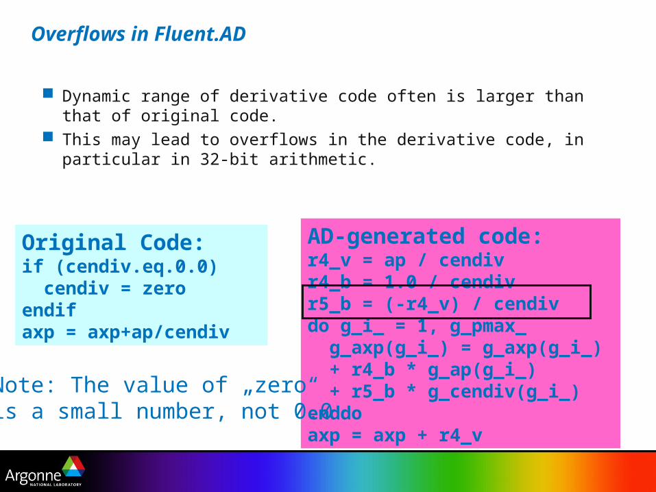
Dynamic range of derivative code often is larger than that of original code. This may lead to overflows in the derivative code, in particular in 32-bit

arithmetic.

Original Code:if (cendiv.eq.0.0) cendiv = zeroendifaxp = axp+ap/cendiv

AD-generated code:r4_v = ap / cendivr4_b = 1.0 / cendivr5_b = (-r4_v) / cendivdo g_i_ = 1, g_pmax_ g_axp(g_i_) = g_axp(g_i_) + r4_b * g_ap(g_i_) + r5_b * g_cendiv(g_i_)enddoaxp = axp + r4_v

Note: The value of „zero“is a small number, not 0.0

Overflows in Fluent.AD

Wisconsin Sea Ice Model

Chain rule (non-)differentiability

if (x .eq. 1.0) then a = yelse if ((x .eq. 0.0) then a = 0else a = x*yendif

b = sqrt(x**4 + y**4)

Mathematical Challenges

Derivatives of intrinsic functions at points of non-differentiability Derivatives of implicitly defined functions Derivatives of functions computed using numerical methods

Due to intrinsic functions– Several intrinsic functions are defined at points where their derivatives are not, e.g.:

• abs(x), sqrt(x) at x=0• max(x,y) at x=y

– Requirements:• Record/report exceptions• Optionally, continue computation using some generalized gradient

– ADIFOR/ADIC approach• User-selected reporting mechanism• User-defined generalized gradients, e.g.:

– [1.0,0.0] for max(x,0)– [0.5,0.5] for max(x,y)

• Various ways of handling– Verbose reports (file, line, type of exception)– Terse summary (like IEEE flags)– Ignore

Due to conditional branches– May be able to handle using trust regions

Points of Nondifferentiability

Implicitly Defined Functions

– Implicitly defined functions often computed using iterative methods

– Function and derivatives may converge at different rates

– Derivative may not be “accurate” if iteration halted upon function convergence

– Solutions:•Tighten function convergence criteria•Add derivative convergence to stopping criteria•Compute derivatives directly, e.g. A x = b

Derivatives of Functions Computed Using Numerical Methods

Differentiation and approximation may not commute Need to be careful about how derivatives of numerical approximations are

used E.g., differentiating through an ODE integrator can provide unexpected

results due to feedback induced by adaptive stepsize control:

p

zt

t

zz

1

11

11

CVODE_S: Objective

ODE Solver(CVODE)

F(y,p)

y|t=0

py|t=t1, t2, ...

SensitivitySolver

y|t=0

p y|t=t1, t2, ...

dy/dp|t=t1, t2, ...

automatically

Possible Approaches

ad_CVODE

ad_F(y,ad_y,p,ad_p)

y, ad_y|t=0

p,ad_py, ad_y|t=t1, t2, ...

CVODE_Sy|t=0

py, dy/dp |t=t1, t2, ...

ad_F(y,ad_y,p,ad_p)

Apply AD to CVODE:

Solve sensitivity eqns:

Augmented ODE initial-value problem:

,1

mw

w

y

Y

mmm p

fpw

yf

pf

pwyf

pytf

pYtF

111

),,(

),,(

.)( with ),,( 00 YtYpYtFY

,1

mw

w

y

Y

CVODE as ODE + sensitivity solver

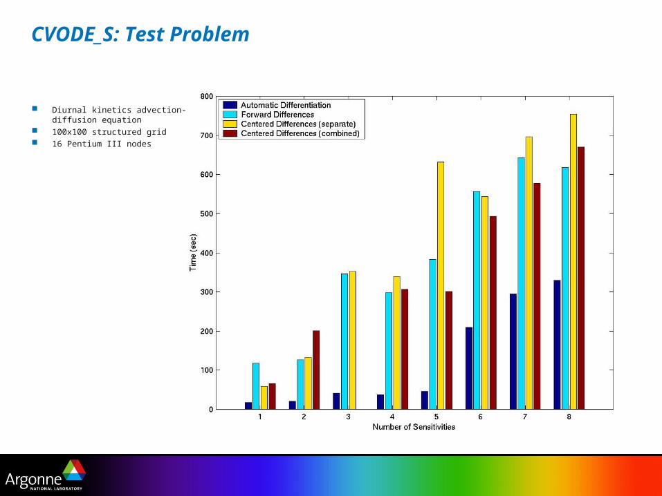
CVODE_S: Test Problem

Diurnal kinetics advection-diffusion equation

100x100 structured grid 16 Pentium III nodes

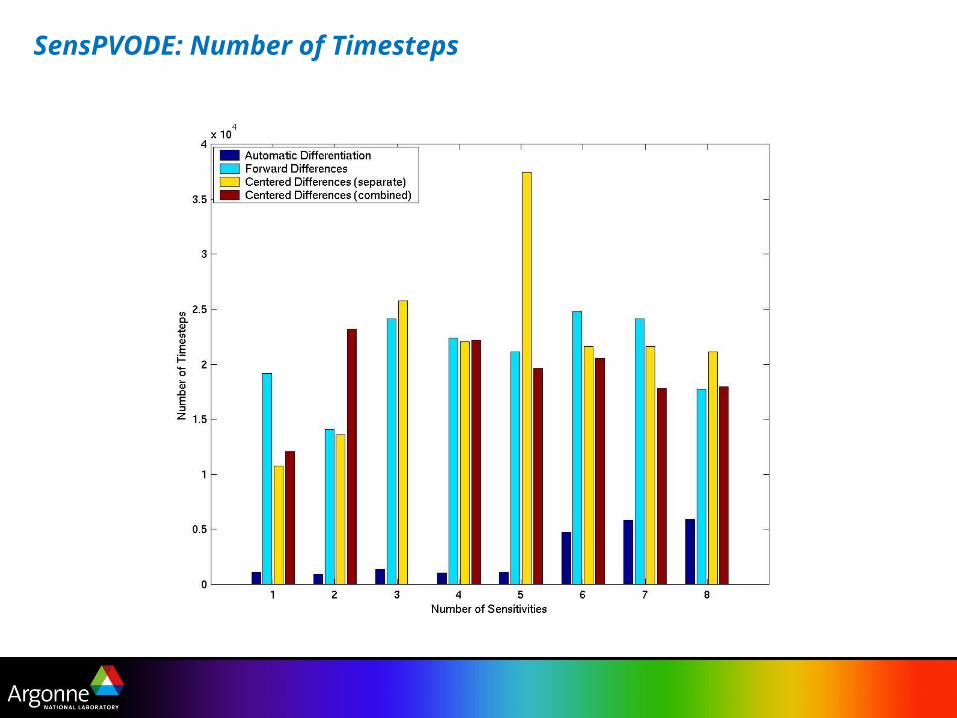
SensPVODE: Number of Timesteps

SensPVODE: Time/Timestep

Addressing Limitations in Black Box AD

Detect points of nondifferentiability

– proceed with a subgradient

– currently supported for intrinsic functions, but not conditional statements

Exploit mathematics to avoid differentiating through an adaptive algorithm Modify termination criterion for implicitly defined functions

– Tighten tolerance

– Add derivatives to termination test (preferred)

Conclusions

There are some potential “gotchas” when applying AD in a black box fashion

Some care should be taken to ensure that the desired quantity is computed

There are usually workarounds

AD Intro: Follow Up

Practical Matters: constructing computational graphs

At compile time (source transformation)

– Structure of graph is known, but edge weights are not: in effect, implement inspector (symbolic) phase at compile time (offline), executor (numeric) phase at run time (online)

– In order to assemble graph from individual statements, must be able to resolve aliases, be able to match variable definitions and uses

– Scope of computational graph construction is usually limited to statements or basic blocks

– Computational graph usually has O(10)—O(100) vertices At run time (operator overloading)

– Structure and weights both discovered at runtime

– Completely online—cannot afford polynomial time algorithms to analyze graph

– Computational graph may have O(10,000) vertices

Checkpointing real applications

In practice, need a combination of all of these techniques At the timestep level, 2- or 3-level checkpointing is typical: too many

timesteps to checkpoint every timestep At the call tree level, some mixture of joint and split mode is desirable

– Pure split mode consumes too much memory

– Pure joint mode wastes time recomputing at the lowest levels of the call tree

Currently, OpenAD provides a templating mechanism to simplify the use of mixed checkpointing strategies

Future research will attempt to automate some of the checkpointing strategy selection, including dynamic adaptation

What to do for very large, dense Jacobian matrices?

Jacobian matrix might be large and dense, but “effectively sparse”

– Many entries below some threshold ε (“almost zero”)

– Can tolerate errors up to δ in entries greater than ε

– Example: advection-diffusion for finite time step: nonlocal terms fall off exponentially

– Solution: do a partial coloring to compress this dense Jacobian: requires solving a modified graph coloring problem

Jacobian might be large and dense, but “effectively low rank”

– Can be well approximated by a low rank matrix

– Jacobian-vector products (and JTv) are cheap

– Adaptation of efficient subspace method uses Jv and JTv in random directions to build low rank approximation (Abdel-Khalik et al., AD08)

Application highlights

Atmospheric chemistry Breast cancer biostatistical analysis CFD: CFL3D, NSC2KE, (Fluent 4.52: Aachen) ... Chemical kinetics Climate and weather: MITGCM, MM5, CICE Semiconductor device simulation Water reservoir simulation

Tuned parameters Standard parameters

- Simulated (yellow) and observed (green) March ice thickness (m)

Parameter tuning: sea ice model

Differentiated Toolkit: CVODES (nee SensPVODE)

Diurnal kinetics advection-diffusion equation

100x100 structured grid 16 Pentium III nodes

Sensitivity Analysis: mesoscale weather model

Conclusions & Future Work

Automatic differentiation research involves a wide range of combinatorial problems

AD is a powerful tool for scientific computing Modern automatic differentiation tools are robust and produce efficient

code for complex simulation codes

– Robustness requires an industrial-strength compiler infrastructure

– Efficiency requires sophisticated compiler analysis Effective use of automatic differentiation depends on insight into problem

structure Future Work

– Further develop and test techniques for computing Jacobians that are effectively sparse or effectively low rank

– Develop techniques to automatically generate complex and adaptive checkpointing strategies

For More Information

Andreas Griewank, Evaluating Derivatives, SIAM, 2000. Griewank, “On Automatic Differentiation”; this and other technical reports

available online at: http://www.mcs.anl.gov/autodiff/tech_reports.html AD in general: http://www.mcs.anl.gov/autodiff/, http://www.autodiff.org/ ADIFOR: http://www.mcs.anl.gov/adifor/ ADIC: http://www.mcs.anl.gov/adic/ OpenAD: http://www.mcs.anl.gov/openad/ Other tools: http://www.autodiff.org/ E-mail: hovland@mcs.anl.gov