00,% ~ S | NSUPPER8 10B12 14 162OUNDF IG. 1 COMPARISONOFREF. I

uJcto-0& ~~~~~~UPPER

__ BOUNND P36-6

o ACTUAL-7

8 10 12 14 16 18 20

SNR db

FIG. I COMPARISON OF 'DIFFEREN4T?5OUNDS FOR N 1O

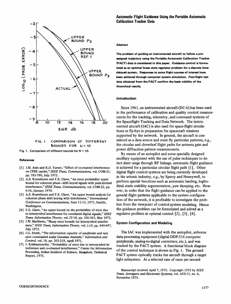
Fig. 1. Comparison of different bounds forN = 10.

References

[1] J.M. Aein and R.D. Turner, "Effect of co-channel interferenceon CPSK carrier," IEEE Trans. Communications, vol. COM-21,pp. 783-790, July 1973.

[2] A.S. Rosenbaum and F.E. Glave, "An error probability upperbound for coherent phase-shift keyed signals with peak-limitedinterference," IEEE Trans Communications, vol. COM-22, pp.6-16, January 1974.

[3] A.S. Rosenbaum and F.E. Glave, "An upper bound analysis forcoherent phase shift keying with interference," InternationalConference on Communications, June 11-13, 1973, Seattle,Washington.

[41 F.E. Glave, "An upper bound on the probability of error dueto intersymbol interference for correlated digital signals," IEEETransa Information Theory, vol. IT-18, pp. 356-363, May 1972.

[5] J.W. Matthews, "Sharp error bounds for intersymbol interfer-ence," IEEE Trans. Information Theory, vol. I-19, pp. 440447,July 1973.

[6] J.G. Smith, "fThe information capacity of amplitude and vari-ance constrained scalar Gaussian channels," Information andControl, vol. 18, pp. 203-219, April 1971.

[7] J. Krishnamurthy, "Probability of error due to intersymbol in-terference and co-channel interference," Center for InformationProcessing, Indian Institute of Science, Bangalore, TechnicalReport, 1975.

Automatic Flight Guidance Using the Portable AutomaticCalibration Tracker Data

Abstract

The problem of guiding an instrumented aircraft to follow a pre-

assigned trajectory using the Portable Automatic Calibration Tracker(PACT) data is considered in this paper. Guidance control is formu-lated as an optimal linear state regulator problem for a discrete time-delayed system. Responses to some flight courses of interest have,been achieved through computer system simulation. Post-flight testdata obtained from the PACT confirm the basic validity of thetheoretical results.

Introduction

Since 1961, an instrumented aircraft (DC-6) has been usedin the performance of calibration and quality control measure-ments for the tracking, telemetry, and command systems ofthe Spaceflight Tracking and Data Network. The instru-mented aircraft (IAC) is also used for space-flight simula-tions or fly-bys in preparation for spacecraft missionssupported by the network. In general, the aircraft is con-sidered as a data source and must fly particular patterns, e.g.,the circular and cloverleaf flight paths for antenna gain andpower diffraction pattern measurements.

By means of an autopilot and some specially designedancillary equipment with the use of pulse techniques to de-tect slant range through RF linkage, automatic flight guidanceis achieved for a particular circular flight path [1]. Otherdigital flight control systems are being currently developedin the avionic industry, e.g., by Sperry and Honeywell, toperform special functions such as automatic landing, logitu-dinal static stability argumentation, yaw damping, etc. How-ever, in order that the flight guidance can be applied to thegenerWl flight patterns applicable to the system configura-tion of the network, it is profitable to investigate the prob-lem from the viewpoint of control Isystem modeling. Hencethe guidance problem can be formulated and solved as a

regulator problem in optimal control [2], [3], [4].

System Configuration and Modeling

The IAC was implemented with the autopilot, airbornedata-processing equipment (digital DDP-5 16 computerperipherals, analog-to-digital converters, etc.), and wastracked by the PACT system. A functional block diagramof the control technique is shown in Fig. 1. The groundPACT system optically tracks the aircraft through a targetlight subsystem. At a selected rate of once per second

Manuscript received April 7, 1975. Copyright 1975 by IEEETrans. Aerospace and Electranic Systems, vol AES-11, no. 6,November 1975.

CORRESPONDENCE 1377

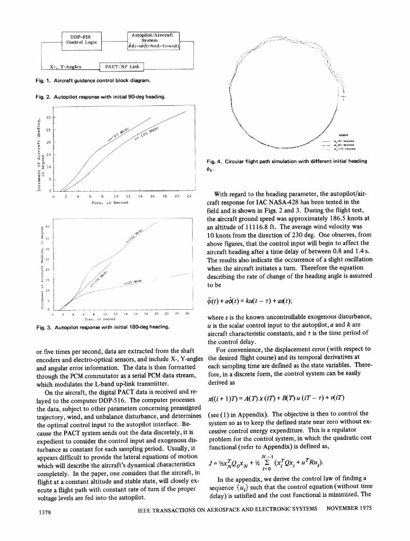
Fig. 1. Aircraft guidance control block diagram.

Fig. 2. Autopilot response with initial 90-deg heading.

. 30

10 25.,8X 20

:

X 10

a~44 .H

5444L

H O

0i=90 d.gre..6.80 d.gr...O 100 degrees

0 2 4 6 8 10 12 14 16 18 20

Time, in Second

(D 40

3

03 0

a,> 30 /

G 25

20

"1 5 c_25M

0 2 4 6 8 10 12 14 16 18 20 22 24 26

Time, in Second

Fig. 3. Autopilot response with initial 180-deg heading.

or five times per second, data are extracted from the shaftencoders and electro-optical sensors, and include X-, Y-anglesand angular error information. The data is then formattedthrough the PCM commutator as a serial PCM data stream,which modulates the L-band up-link transmitter.

On the aircraft, the digital PACT data is received and re-

layed to the computer DDP-5 16. The computer processes

the data, subject to other parameters concerning preassignedtrajectory, wind, and unbalance disturbance, and determinesthe optimal control input to the autopilot interface. Be-cause the PACT system sends out the data discretely, it is

expedient to consider the control input and exogenous dis-

turbance as constant for each sampling period. Usually, it

appears difficult to provide the lateral equations of motionwhich will describe the aircraft's dynamical characteristicscompletely. In the paper, one considers that the aircraft, in

flight at a constant altitude and stable state, will closely ex-

ecute a flight path with constant rate of turn if the proper

voltage levels are fed into the autopilot.

Fig. 4. Circular flight path simulation with different initial heading

'o

With regard to the heading parameter, the autopilot/air-craft response for IAC NASA428 has been tested in thefield and is shown in Figs. 2 and 3. During the flight test,

the aircraft ground speed was approximately 186.5 knots at

an altitude of 1 1 1 16.8 ft. The average wind velocity was

10 knots from the direction of 230 deg. One observes, fromabove figures, that the control input will begin to affect theaircraft heading after a time delay of between 0.8 and 1.4 s.

The results also indicate the occurrence of a slight oscillationwhen the aircraft initiates a turn. Therefore the equationdescribing the rate of change of the heading angle is assumedto be

¢(t) + a4t) = kul(t - r) + as(t);

where s is the known uncontrollable exogenous disturbance,u is the scalar control input to the autopilot, a and k are

aircraft characteristic constants, and r is the time period ofthe control delay.

For convenience, the displacement error (with respect to

the desired flight course) and its temporal derivatives at

each sampling time are defined as the state variables. There-

fore, in a discrete form, the control system can be easilyderived as

x((i + 1)1) = A(T)x(i) + B(T) u (iT- r) + v(iT)

(see (1) in Appendix). The objective is then to control the

system so as to keep the defined state near zero without ex-

cessive control energy expenditure. This is a regulatorproblem for the control system, in which the quadratic cost

functional (refer to Appendix) is defined as,

N-1

J-½,.xkNQoxN + Ih z (xi Qxi +uRu).1=0

In the appendix, we derive the control law of finding a

sequence {uiJ such that the control equation (without time

delay) is satisfied and the cost functional is minimized. The

IEEE TRANSACTIONS ON AEROSPACE AND ELECTRONIC SYSTEMS NOVEMBER 1975

,'.f

If I

.r

1378

/00 0 0\Q00 = 0 4 0J

(1 4 0, R=1400

(100 0____ =0 = t 0 30 °0 R= 20o 00 0o

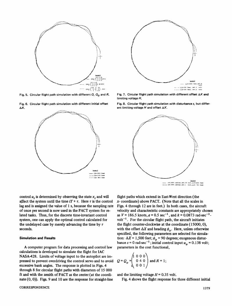
Fig. 5. Circular flight path simulation with different Q, QO and R.

Fig. 6. Circular flight path simulation with different initial offsetAX.

- a X= 1500 feet, H=n .4..It

-- - A, X=750 feet, H=0 3 .1ltAX=350 fe .t,H=0.42,It

Fig. 7. Circular flight path simulation with different offset AX andlimiting voltage H.

Fig. 8. Circular flight path simulation with disturbance s, but differ-ent limiting voltage H and offset AX.

Legend

ZIX- 1500 feet

--_AX=1100 feet----- OX= SOO fe-t

L.q..d- -0.009 X4d/.e.H9-0.35 olt,XAX=1500 fe.t

_- s-0.009 rad/.ec,H-0.1 XOlt,AX= 750 f.,t

control ui is determined by observing the state xi and willagfect the system until the time iT + r. Here r is the controllag and is assigned the value of 1 s, because the sampling rateof once per second is now used in the PACT system for re-lated tasks. Thus, for the discrete time-invariant controlsystem, one can apply the optimal control calculated forthe undelayed case by merely advancing the time by rseconds.

Simulation and Results

A computer program for data processing and control lawcalculations is developed to simulate the flight for IACNASA428. Limits of voltage input to the autopilot are im-pressed to prevent overdriving the control servo and to avoidexcessive bank angles. The response is plotted in Figs. 4through 8 for circular flight paths with diameters of 15 000ft and with the zenith of PACT as the center (at the coordi-nate (0, 0)). Figs. 9 and 10 are the response for straight-line

flight paths which extend in East-West direction (thex- coordinate) above PACT. (Note that all the scales inFigs. 4 through 12 are in feet.) In both cases, the aircraftvelocity and characteristic constants are appropriately chosenas V = 186.5 knots, a = 0.5 sec' , and k = 0.0873 rad-sec2-volt'1 . For the circular flight path, the aircraft initiatesthe flight counter-clockwise at the coordinate ( 15000, 0),with the offset AX and heading (,e. Here, unless otherwisespecified, the following parameters are selected for simula-tion: AX = 1,500 feet; 00 = 90 degrees; exogenous distur-bance s = O rad-sec1 ; initial control input u0 = 0.138 volt;parameters in the cost functional,

/10 0 0\Q=QO = 040 andR=1;

0 0 1

and the limiting voltageH = 0.35 volt.Fig. 4 shows the flight response for three different initial

CORRESPONDENCE 1379

4000. --

~/-~ -- >,f-L.egend

/10 0 0\

/10 0 0\Q=Q1 0 4 0), R=104o

\ 00 1

~~~~Q=Qo=h0 o I-----Q=Q- A00 0 izy\, Ro0 30 00 0 10

I1 I I-60000. -50000. -40D00- -30000. -20000. -10000.

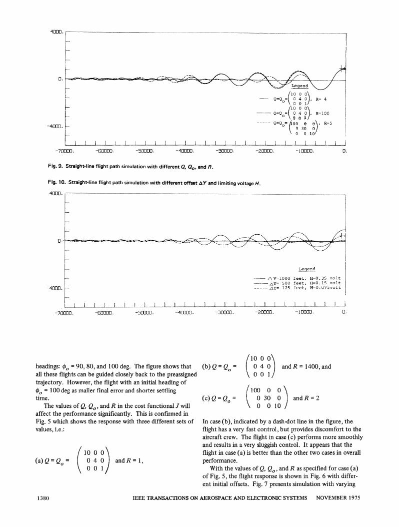
Fig. 9. Straight-line flight path simulation with different 0, 00, and R.

Fig. 10. Straight-line flight path simulation with different offset AY and limiting voltage H.

4000.

O.,

Legend

Z\Y=1000 feet, H=0.35 volt---,Y= 500 feet, H=0. 15 volt

-- nY= 125 feet, H=U.U75volt-4000. P-

I-60000. -50000. -40000. -30000.

_I_ L-20000. -10000. 0.

headings: b0, = 90, 80, and 100 deg. The figure shows thatall these flights can be guided closely back to the preassignedtrajectory. However, the flight with an initial heading of00 = 100 deg as maller final error and shorter settlingtime.

The values of Q, Q0, and R in the cost functional J willaffect the performance significantly. This is confirmed inFig. 5 which shows the response with three different sets ofvalues, i.e.:

(10 00,(a)Q=Q= l 04 ° andR =l1

000 1/

(b) Q = Q =

(c)Q=QQ =

(10 0 0\0 4 00 0 1/

(100 00 300 0

00

10

and R = 1400, and

i and R = 2

In case (b), indicated by a dash-dot line in the figure, theflight has a very fast control, but provides discomfort to theaircraft crew. The flight in case (c) performs more smoothlyand results in a very sluggish control. It appears that theflight in case (a) is better than the other two cases in overall

performance.With the values of Q, QO, and R as specified for case (a)

of Fig. 5, the flight response is shown in Fig. 6 with differ-ent initial offsets. Fig. 7 presents simulation with varying

IEEE TRANSACTIONS ON AEROSPACE AND ELECTRONIC SYSTEMS NOVEMBER 1975

0.

-4000.

-70000. 0.

-70000.

Z; Pp-%- I-_Aovlnm w_-wos:s---Z_-- 49-;> .,-= w"i-, --A t, A--~- 1 :

<----- --;.; - ol,. - =ar.. ---.

fI -I

/ 1--,/

1 380

1*11117-.--

202100.

0.

-2000. K

-4000. L 1 LI.LL LL I l l-14000. -000. -2000. 4000.

Legend-1 -1a=0.5 sec k=0.0873 rad volt 2

sec10 0 0

Q=Q0= 0 4 01, R=4, H=0.025 voltQ \Q 001/

LlIIWIIL10000.

116000.

1-122000.

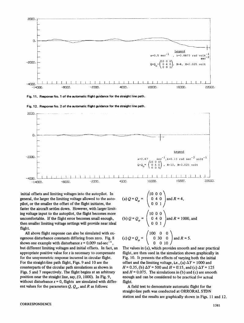
Fig. 11. Response No. 1 of the automatic flight guidance for the straight line path.

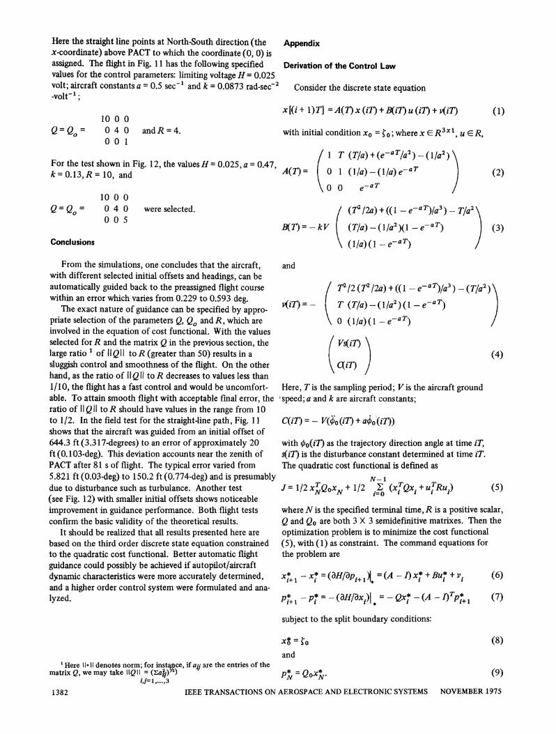
Fig. 12. Response No. 2 of the automatic flight guidance for the straight line path.

2000. r-

0. e

-2000. Ka=0.4 7 sec

/10 0 0

° 0 G)

-4000 1. 1- L I _I-14000. -5000. -2000. 4000.

initial offsets and limiting voltages into the autopilot. Ingeneral, the larger the limiting voltage allowed to the auto-pilot, or the smaller the offset of the flight initiates, thefaster the aircraft settles down. However, with larger limit-ing voltage input to the autopilot, the flight becomes moreuncomfortable. If the flight error becomes small enough,then smaller limiting voltage settings will provide near idealflight.

All above flight response can also be simulated with ex-ogenous disturbance constants differing from zero. Fig. 8shows one example with disturbance s = 0.009 rad-sec1,but different limiting voltages and initial offsets. In fact, anappropriate positive value for s is necessary to compensatefor the unsymmetric response incurred in circular flight.For the straight-line path flight, Figs. 9 and 10 are thecounterparts of the circular path simulations as shown inFigs. 5 and 7 respectively. The flight begins at an arbitraryposition near the straight line, say, (0, 1000). In Fig. 9,without disturbance s = 0, flights are simulated with differ-ent values for the parameters Q, QO, and R as follows:

(a) Q =

(b)Q=Qo =

II10000.

(1000

(10l

040

040

001

001

Legend

- 1 -2 -,I,k=0.13 rad sec volt

, R=10, H=0.025 volt

I I_L I.16000. 22000.

)andR =4,

)and R =1000, and

(100 0 0(c)Q=Q= 0 30 0 andR=5.

0~ 00\ 0 101The values in (a), which provides smooth and near practicalflight, are then used in the simulation shown graphically inFig. 10. It presents the effects of varying both the initialoffset and the limiting voltage, ie., (a) AY = 1000 andH= 0.35,(b) AY= 500 andH= 0:15, and(c) AY= 125andH = 0.075. The simulations in (b) and (c) are smoothenough and can be considered to be practical for actualflight.A field test to demonstrate automatic flight for the

straight-line path was conducted at ORRORAL STDNstation and the results are graphically shown in Figs. 1 1 and 12.

CORRESPONDENCE

I 11-

1381

lIere the straight line points at North-South direction (thex-coordinate) above PACT to which the coordinate (0, 0) isassigned. The flight in Fig. 11 has the following specifiedvalues for the control parameters: limiting voltage H = 0.025volt; aircraft constants a = 0.5 sec- 1 and k = 0.0873 rad-sec-2-volt 1;

10 0 0Q=Q= 04 0 andR=4.

00O 0 1

For the test shown in Fig. 12, the values H = 0.025, a = 0.47,k=0.13,R= 10, and

10 0 0QQO = 0 4 0 were selected.Cocl 005

Conclusions

Appendix

Derivation of the Control Law

Consider the discrete state equation

x [(i + 1)T] = A( x (i) +BiT) u (i) +vi) (1)

with initial condition x0 = T0; where x E R3x1, u ER,

(Tla) + (e aT/a2) - (Il/a2)(I/a) -(l/a) e-aT

e-aT /

/1 T

A(Y) = 0 1

0O

B(7)=-kV(

(2)

(7T2/2a) + (( 1-e-a T)Ia3)_ T/a2\

(T/a)-(l/a2)(I - e-aT) | (3)(I/a)(- e-aT) /

From the simulations, one concludes that the aircraft,with different selected initial offsets and headings, can beautomatically guided back to the preassigned flight coursewithin an error which varies from 0.229 to 0.593 deg.

The exact nature of guidance can be specified by appro-priate selection of the parameters Q, QO and R, which areinvolved in the equation of cost functional. With the valuesselected for R and the matrix Q in the previous section, thelarge ratio l of II QI to R (greater than 50) results in asluggish control and smoothness of the flight. On the otherhand, as the ratio of IIQII to R decreases to values less than1/10, the flight has a fast control and would be uncomfort-able. To attain smooth flight with acceptable final error, theratio of 1 Q11 to R should have values in the range from 10to 1/2. In the field test for the straight-line path, Fig. 11shows that the aircraft was guided from an initial offset of644.3 ft (3.317-degrees) to an error of approximately 20ft (0.1 03-deg). This deviation accounts near the zenith ofPACT after 81 s of flight. The typical error varied from5.821 ft (0.03-deg) to 150.2 ft (0.774-deg) and is presumablydue to disturbance such as turbulance. Another test(see Fig. 12) with smaller initial offsets shows noticeableimprovement in guidance performance. Both flight testsconfirm the basic validity of the theoretical results.

It should be realized that all results presented here arebased on the third order discrete state equation constrainedto the quadratic cost functional. Better automatic flightguidance could possibly be achieved if autopilot/aircraftdynamic characteristics were more accurately determined,and a higher order control system were formulated and ana-lyzed.

1 Here 11-11 denotes norm; for inst;ce, if aij are the entries of thematrix Q, we may take IIQII = (Lap)) )

i,j=l,...,3

and

1/2 (r 12a) + ((I1-Te-aT))a3)_(Ta2)V(iT) =- |T (Tla)-_( l/a2) (I e-aT)l

\0 (Il/a)(l-e-aT)/

Vs(iT)

C(iI) ) (4)

Here, T is the sampling period; V is the aircraft ground-speed; a and k are aircraft constants;

C(iT) = - V(40 (ii) + aOb (if))

with 0o(iT) as the trajectory direction angle at time iT,s(il) is the disturbance constant determined at time iT.The quadratic cost functional is defined as

N-1JI 1/2xTQOXN + 1I2 i2 (xTQx + I RuT )N N i=0 ' (5)

whereN is the specified terminal time,R is a positive scalar,Q and Qo are both 3 X 3 semidefmnitive matrixes. Then theoptimization problem is to minimize the cost functional(5), with (1) as constraint. The command equations forthe problem are

(6)

(7)

Xi+ 1 -.x = (W3pi,, = (A -I X* + Bu +v .

P* _ P ==-(Walaxi)l = -Qx -(A - f)TP*

subject to the split boundary conditions:

xt = to

and

pN = QOx*.

(8)

(9)

IEEE TRANSACTIONS ON AEROSPACE AND ELECTRONIC SYSTEMS NOVEMBER 19751382

Minimizing the Hamiltonian yields

u* =-RlBTp *

with the costate p* of the form

p* = Kx* + g (1 1)

Thus, combining ( 10), ( 1 1), (6), and (7), rearranging andsimplifying terms gives

U= -(R + BTK.+ TB)-3BTKi+ Ax!

+ (R + BTKi+B)-'BTK. BR-1BT

R-lBTg1 -(R + BTK lB)lBTK+vt (12)

Here Ki and gi are the solutions of the following equations:

K= Q+ATK+A-ATK,+1B(R +BTKE JB)-BTKI+ A

[51 J. Tyler, Jr., "The characteristics of model-following system assynthesized by optimal control," IEEE Trans Automat. Contr.,

(10) vol. AC-9, October 1964.[6] K.Astron, Introduction to Stochastic Control Theory, New York:

Academic Press, 1970.[7] B. Keiser, "Unified control system," IEEE Trans Aerospace and

Electronic Systems, vol. AES-7, September 1971.

Location Estimation and Guidance Using Radar Imagery

Abstract

Radar map-matching location-estimation systems compare radar

images of the terrain with a memory "map" to obtain an estimate

of sensor position in the mapped area for guidance.

This correspondence summarizes a data-acquisition program in-

volving an omnidirectional range-scan radar sensor, and presents re-

sults of theoretical guidance exercises based on comparing actual

radar signals with computer-generated memories.

= Q + (A - BrI)TK,+ A Introduction

= (A - BrI)TK+1(A - BrI) + rLRr. + Q (13)

gj=ATK (I-B(R +BTK.+lB)lBTK+l)Vi-4 Ki+ 1(I-B(R + BTKi+ B)-

BTK. 1)BRl1BTg1 +ATg1BK+ 1wR-lBgi + A gi+

where

ri = (R + BTKi+ 1B)-BTKj+ 1A. (14)

Acknowledgment

The author would like to thank Phil C. Davis for hisassistance in computer simulation and helpful commentsduring this work.

CHING-TAI LINBendix Field Engineering Corp.Columbia, Md. 21045

References

[1] "Circular Flight Path System," Part II of the Apollo SpacecraftSimulation System, the Bendix Corporation, Bendix RadioDivision, Baltimore, Maryland, Contract NAS5-10750, April1970.

[2] H. Halkin, "A maximum principle of the pontryagin type forsystem described by nonlinear difference equations," SIAM J.Contr., vol. 4, no. 1, 1966.

[3] M. Athans and P. Falb, Optimal Control-An Introduction to theTheory and Its Applications, New York: McGraw-Hill, 1966.

[4] R. Pindyck, "An application of linear quadratic tracking prob-lem to economic stabilization policy," IEEE Trans. Automat.Contr., vol. AC-17, June 1972.

Accurate location and guidance techniques for missiles,RV's, and aircraft are of increasing interest as technologicaldevelopments enable more sophisticated and powerful sys-tem concepts. Radar imagery offers a promising approachbecause of the potential for high accuracy and essentiallyall-weather operation without any requirement for associ-ated ground equipment. In several radar location andguidance concepts, [1-7] , radar images (for example, thereturned power waveform resulting from a transmittedradar pulse) are compared with information stored in memoryso that location can be estimated through a map-matchingor correlation process.

If the images are generated by scanning narrow-beamantenna patterns across a scene, the process is somewhatanalogous to two-dimensional optical location estimation[8]. However, narrow-beam antenna patterns are achievedat the expense of physical size and usually result in orienta-tion and control problems. Wide-beam antenna patterns,on the other hand, sacrifice resolution and power density.However, even omnidirectional antenna patterns yield auseful amount of resolution for reasonably small pulsewidths, because the time location of significant variationsin the reflected energy depends on the range to the featuresresponsible for the perturbations. The simplicity of wide-beam antennas may result in a unique potential for applica-tions where antenna size and complexity are limited byother design considerations.

Manuscript received December 16, 1974. Copyright 1975 byIEEE Trans. Aerospace and Electronic Systems, vol. AES-11, no. 6,November 1975.

This work was supported by the U.S. Energy Research andDevelopment Administration.

CORRESPONDENCE 1383