automatic optimization of thread-coarsening for...
TRANSCRIPT
Automatic Optimization of Thread-Coarsening for GraphicsProcessors
Alberto MagniSchool of Informatics
University of EdinburghUnited Kingdom
Christophe DubachSchool of Informatics
University of EdinburghUnited Kingdom
Michael O’BoyleSchool of Informatics
University of EdinburghUnited Kingdom
ABSTRACTOpenCL has been designed to achieve functional portabilityacross multi-core devices from different vendors. However,the lack of a single cross-target optimizing compiler severelylimits performance portability of OpenCL programs. Pro-grammers need to manually tune applications for each spe-cific device, preventing effective portability. We target acompiler transformation specific for data-parallel languages:thread-coarsening and show it can improve performance acrossdifferent GPU devices. We then address the problem of se-lecting the best value for the coarsening factor parameter,i.e., deciding how many threads to merge together. We ex-perimentally show that this is a hard problem to solve: goodconfigurations are difficult to find and naive coarsening infact leads to substantial slowdowns. We propose a solutionbased on a machine-learning model that predicts the bestcoarsening factor using kernel-function static features. Themodel automatically specializes to the different architecturesconsidered. We evaluate our approach on 17 benchmarks onfour devices: two Nvidia GPUs and two different generationsof AMD GPUs. Using our technique, we achieve speedupsbetween 1.11× and 1.33× on average.
1. INTRODUCTIONGraphical Processing Units (GPUs) are widely used for
high performance computing. They provide cost-effectiveparallelism for a wide range of applications. The success ofthese devices has lead to the introduction of a diverse rangeof architectures from many hardware manufacturers. Thishas created the need for a common programming language toharness the available parallelism in a portable way. OpenCLis an industry-standard language for GPUs that offers pro-gram portability across accelerators of different vendors: asingle piece of OpenCL code is guaranteed to be executableon many diverse devices.
A uniform language specification, however, still requiresprogrammers to manually optimize kernel code to improveperformance on each target architecture. This is a tedious
.
process, which requires knowledge of hardware behavior, andmust be repeated each time the hardware is updated. Thisproblem is particularly acute for GPUs which undergo rapidhardware evolution.
The solution to this problem is a cross-architectural opti-mizer capable of achieving performance portability. Currentproposals for cross-architectural compiler support [21, 34] allinvolve working on source-to-source transformations. Com-piler intermediate representations [6] and ISAs [5] that spanacross devices of different vendors have still to reach fullsupport.
This paper studies the issue of performance portability fo-cusing on the optimization of the thread-coarsening compilertransformation. Thread coarsening [21, 30, 31] merges to-gether two or more parallel threads, increasing the amountof work performed by a single thread, and reducing the totalnumber of threads instantiated. Selecting the best coarsen-ing factor, i.e., the number of threads to merge together, isa trade-off between exploiting thread-level parallelism andavoiding execution of redundant instructions. Making thecorrect choice leads to significant speedups on all our plat-forms. Our data show that picking the optimal coarseningfactor is difficult since most configurations lead to perfor-mance downgrade and only careful selection of the coarsen-ing factor gives improvements. Selecting the best parameterrequires knowledge of the particular hardware platform, i.e.,different GPUs have different optimal factors
In this work we select the coarsening factor using an au-tomated machine learning technique. We build our modelbased on a cascade of neural networks that decide whetherit is beneficial to apply coarsening. The inputs to the modelare static code features extracted from the parallel OpenCLcode. These features include, among the others, branch di-vergence and instruction mix information. The techniqueis applied to four GPU architectures: Fermi and Keplerfrom Nvidia and Cypress and Tahiti from AMD. While naivecoarsening misses optimization opportunities, our approachgives an average performance improvement of 1.16x, 1.11x,1.33x, 1.30x respectively.
In summary the paper makes the following contributions:
• We provide a characterization of the optimization spaceacross four architectures.
• We develop a machine learning technique based on aneural network to predict coarsening.
• We show significant performance improvements across17 benchmarks
The remainder of the paper is organized as follows. Sec-tion 2.1 provides a brief overview of OpenCL and describesthe thread coarsening transformation. A motivating exam-ple for the problem is provided in section 3. Section 4 de-scribes the experimental setup and the compiler infrastruc-ture. Section 5 presents a characterization of the optimiza-tion space. Section 6 describes the machine the machinelearning model. The results are presented in Section 7. Sec-tion 8 presents the related work and section 9 concludes thepaper.
2. BACKGROUND
2.1 OpenCLOpenCL is a cross-vendor programming language used for
massively parallel multi-core graphic processors. OpenCLkernel functions define the operations carried out by eachdata-parallel hardware-thread. Kernels are compiled at run-time on the host (a standard CPU) and sent to executiononto the device (in our case a GPU). It is the program-mer’s responsibility to decide how many threads to instan-tiate and how to arrange them into work-groups, definingthe so-called NDRange of thread-ids. Each thread-id cor-responds to thread executing within a work-group. Work-items in a work-group are guaranteed to be scheduled ontoa single core and can share data in local memory and syn-chronize using barriers.
OpenCL programmers, usually, instantiate as many threadsas they have data element to process. This results in hun-dreds of thousands of threads being scheduled on the tar-get device, maximizing the degree of parallelism. However,there is no guarantee that this policy is the best for eachpossible target device. Consider for instance the presenceof thread-invariant instructions [18, 33] which produces thesame results independently from the thread executing them.Maximizing the number of threads might increase the totalnumber of redundant operations executed by the GPU.
2.2 Thread CoarseningOne way to prevent the problems associated with having
too fine-grained parallelism is to merge threads together.This reduces the redundancy in the number of integer oper-ations and branches performed per floating point operation.This transformation, known as thread coarsening [21, 30,31], works by fusing multiple work items together increasingthe amount of work performed by a single thread and re-ducing the overall number of launched threads. While it ap-pears to be an easy task for the programmer, it is preferableto apply this transformation automatically using a compilerfor two reasons: (1) the merging is done by replicating in-structions inside the kernel, which is error-prone to do byhand; (2) the Coarsening Factor (i.e., the number of timesthe body of the thread is replicated) which gives the bestperformance depends on the program and on the hardware.
The coarsening transformation we implemented increasesthe amount of work performed by the kernel by replicatingthe instructions in its body. Leveraging divergence analy-sis [9, 15, 18] only instructions that depend on the thread-id (divergent instructions) are replicated. This reduces theoverhead of executing uniform instructions across multiplethreads. Divergent instructions are replicated and insertedright after the original ones updating the thread-id to work
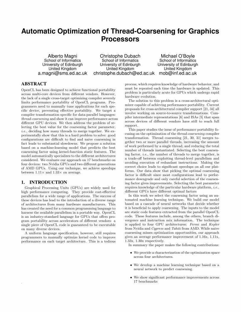
1 kernel void square ( global f loat ∗ in , out ) {2 int g id = g e t g l o b a l i d ( 0 ) ;3 out [ g id ] = in [ g id ]∗ in [ g id ] ; }
(a) Original code
1 kernel void square2x ( global f loat ∗ in , out ) {2 int g id = g e t g l o b a l i d ( 0 ) ;3 int t i d0 = 2∗ g id+0;4 int t i d1 = 2∗ g id+1;5 out [ t i d0 ] = in [ t i d0 ]∗ in [ t i d0 ] ;6 out [ t i d1 ] = in [ t i d1 ]∗ in [ t i d1 ] ; }
(b) After coarsening with factor 2
Figure 1. Vector square example in OpenCL. In the origi-nal code each thread takes the square of one element of theinput array a. When coarsened by a factor two b , eachthread now processes two elements of the input array.
on the correct data elements. Finally, the number of instan-tiated thread is reduced at runtime.
Figure 1 shows a kernel that calculates the square of the el-ement of the input array. In the original code, each thread isresponsible for squaring one element of the input array. Af-ter coarsening has been applied with factor two, each threadprocesses two element of the input array. As can be see onlines 3–4 of figure 1b, the index in the input array are calcu-lated from the original thread iteration space as returned bythe OpenCL get global id(0) function. Prior work on thiscompiler transformation ([21]) presents how to effectivelymanage branches and loops.
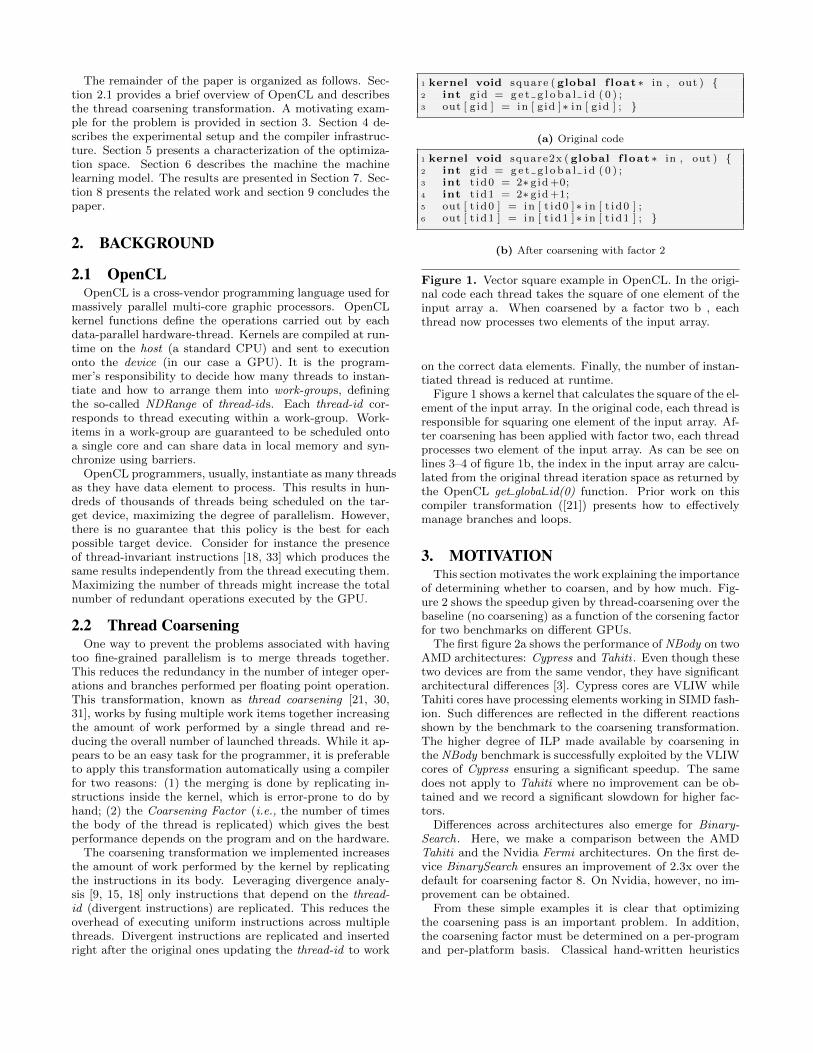
3. MOTIVATIONThis section motivates the work explaining the importance
of determining whether to coarsen, and by how much. Fig-ure 2 shows the speedup given by thread-coarsening over thebaseline (no coarsening) as a function of the corsening factorfor two benchmarks on different GPUs.
The first figure 2a shows the performance of NBody on twoAMD architectures: Cypress and Tahiti . Even though thesetwo devices are from the same vendor, they have significantarchitectural differences [3]. Cypress cores are VLIW whileTahiti cores have processing elements working in SIMD fash-ion. Such differences are reflected in the different reactionsshown by the benchmark to the coarsening transformation.The higher degree of ILP made available by coarsening inthe NBody benchmark is successfully exploited by the VLIWcores of Cypress ensuring a significant speedup. The samedoes not apply to Tahiti where no improvement can be ob-tained and we record a significant slowdown for higher fac-tors.
Differences across architectures also emerge for Binary-Search. Here, we make a comparison between the AMDTahiti and the Nvidia Fermi architectures. On the first de-vice BinarySearch ensures an improvement of 2.3x over thedefault for coarsening factor 8. On Nvidia, however, no im-provement can be obtained.
From these simple examples it is clear that optimizingthe coarsening pass is an important problem. In addition,the coarsening factor must be determined on a per-programand per-platform basis. Classical hand-written heuristics
Speedup
Coarsening Factor1 2 4 8 16 32
0
1
2
3
4
Cypress
Tahiti
(a) NBody run on Cypress and TahitiSpeedup
Coarsening Factor1 2 4 8 16 32
0.5
1
1.5
2
Fermi
Tahiti
(b) BinarySearch run on Fermi and Tahiti
Figure 2. Speedup achieved with thread coarsening as afunction of the coarsening factor for NBody and Binary-Search
Original OpenCL Nvidia
Transformed OpenCL
1. Clang 3. Axtor
4. Proprietary Compiler2. Coarsening
LLVM IR
AMD
Figure 3. Compiler toolchain
are not only complex to develop, but are likely to fail due tothe variety of programs and ever-changing OpenCL devicesavailable.
4. EXPERIMENTAL SETUPThis section describes the compiler toolchain (4.1), the
coarsening stride (4.2), the benchmarks (4.3) and the devicesused in the experiments (4.4).
4.1 Compiler ToolchainOne way to automatically evaluate a compiler transfor-
mation in OpenCL on multiple devices is to use a source-to-source compiler. It avoids the need to have access topotentially properietary compiler internals. Alternative ap-proaches based on SPIR [6] could also be used in the fu-ture, when it is going to reach wide adoption. Figure 3shows our compilation infrastructure. The OpenCL C codeof the target kernel is translated to LLVM bitcode usingthe clang open-source front-end (stage 1). The coarseningtransformation is applied at the LLVM bitcode level (stage2). The transformed LLVM program is then translated backto OpenCL C using the axtor [24] LLVM OpenCL-backend(stage 3). The transformed OpenCL program is then fedinto the hardware vendor proprietary compiler (stage 4) forcode generation.
Program name Source Num. Threads
1) binarySearch AMD SDK 268M2) blackscholes Nvidia SDK 16M3) convolution AMD SDK 6K4) dwtHaar1D AMD SDK 2M5) fastWalsh AMD SDK 33M6) floydWarshall AMD SDK (8K x 8K)7) mriQ Parboil 524K8) mt AMD SDK (4K x 4K)9) mtLocal AMD SDK (4K x 4K)
10) mvCoal Nvidia SDK 16K11) mvUncoal Nvidia SDK 16K12) nbody AMD SDK 131K13) reduce AMD SDK 67M14) sgemm Parboil (3K x 3K)15) sobel AMD SDK (1K x 1K)16) spmv Parboil 262K17) stencil Parboil (3K x 510 x 62)
Table 1. OpenCL applications with the reference numberof threads.
4.2 Coarsening FactorIn this work we address the tuning of the coarsening fac-
tor parameter. The first one controls how many threads tomerge together. For our experiments we allowed this param-eter to have the following values: [1, 2, 4, 8, 16, 32]. Wherecoarsening factor of 1 corresponds to the original program.We limited our evaluations to powers of two since these arethe most widely applicable parameter values, given the refer-ence input sizes for the considered benchmarks. The tuningtechnique in the next chapters can be easily extended tosupport non powers of two.
4.3 BenchmarksWe have used 17 benchmarks from various sources as
shown in table 1. In the case of the Parboil benchmarkswe used the opencl base version. The table also shows theglobal size (total number of threads) used. The baselineperformance reported in the results section is that of thebest work group size as opposed to the default one chose bythe programmer. This is necessary to give a fair compari-son across platforms when the original benchmark is writtenspecifically for one platform. Each experiment has been re-peated 50 times aggregating the results using the median.Previous work ([22]) has shown that the choice for the op-timal coarsening factor is consistent across input sizes. Forthis reason we restricted our analysis to the input size (i.e.,total number of threads running) for the uncoarsened kernellisted in table 1.
4.4 DevicesFor our experiments we used four devices from two ven-
dors. From Nvidia we used GTX480 and Tesla K20c. Thefirst one is based on the Fermi architecture [2] with 15 stream-ing multiprocessors (SM) and 32 CUDA cores for each. TheTesla K20c has the latest Kepler architecture [4]. K20c has13 SMs each with 192 CUDA cores.From AMD we used the Radeon HD 5900 and Tahiti 7970.The first one, codenamed Cypress, has 20 SIMD cores eachwith 16 thread processors, a 5-way VLIW core. The Graph-ics Core Next architecture in Tahiti 7970 is a radical change
bina
rySe
arch
bl
acks
hole
s co
nvol
utio
n dw
tHaa
r1D
fa
stW
alsh
flo
ydW
arsh
all
mriQ
m
t m
tLoc
al
mvC
oal
mvU
ncoa
l nb
ody
redu
ce
sgem
m
sobe
l sp
mv
sten
cil
aggr
egat
e 0
0.5
1
1.5
2
2.5 Speedup
●
●●
●
●
●
●
●
●
●
●
●
●
●●
●
●
●
3.95 3.95
(a) Fermi
bina
rySe
arch
bl
acks
hole
s co
nvol
utio
n dw
tHaa
r1D
fa
stW
alsh
flo
ydW
arsh
all
mriQ
m
t m
tLoc
al
mvC
oal
mvU
ncoa
l nb
ody
redu
ce
sgem
m
sobe
l sp
mv
sten
cil
aggr
egat
e 0
0.5
1
1.5
2
2.5 Speedup
●● ●
●
●●
●
●
●
●
●
●
●
●
●
●
●●
(b) Kepler
bina
rySe
arch
bl
acks
hole
s co
nvol
utio
n dw
tHaa
r1D
fa
stW
alsh
flo
ydW
arsh
all
mriQ
m
t m
tLoc
al
mvC
oal
mvU
ncoa
l nb
ody
redu
ce
sgem
m
sobe
l sp
mv
sten
cil
aggr
egat
e 0
0.5
1
1.5
2
2.5 Speedup
●
● ●
●
●
●
●
● ●
●
●
●
●
●
●
●
● ●
3.21 3.24 3.78 3.78
(c) Cypress
bina
rySe
arch
bl
acks
hole
s co
nvol
utio
n dw
tHaa
r1D
fa
stW
alsh
flo
ydW
arsh
all
mriQ
m
t m
tLoc
al
mvC
oal
mvU
ncoa
l nb
ody
redu
ce
sgem
m
sobe
l sp
mv
sten
cil
aggr
egat
e 0
0.5
1
1.5
2
2.5 Speedup
●
● ●
●
●
●
●● ●
●
●
●
●
●
●
●
●
●
3.4 2.82 12.01 12.01
(d) Tahiti
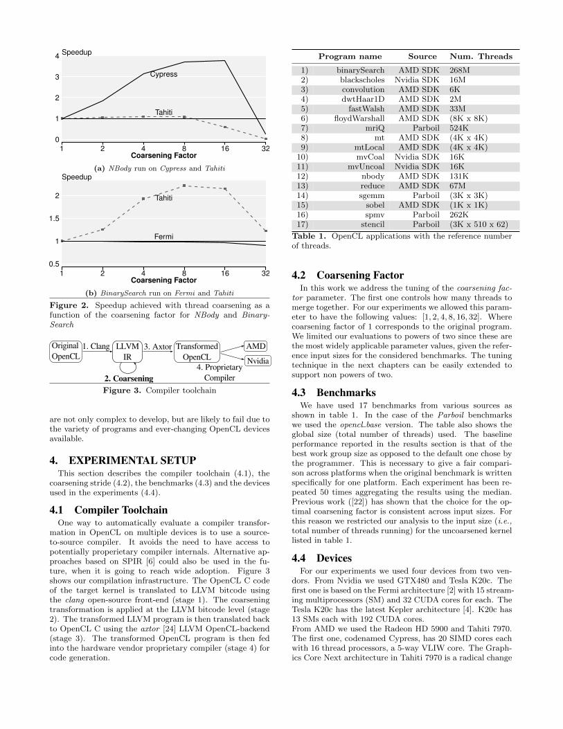
Figure 4. Violin plots showing the distribution of speedups for all the benchmarks on the four devices. The shape of theviolin corresponds to the speedup distribution. They indicate on how hard it is to tune a program. The thick black line showswhere 50% of the data lies. The white dot is the position of the median.
Name Model GPU OpenCL LinuxDriver version kernel
Fermi Nvidia GTX 480 304.54 1.1 CUDA 5.0.1 3.2.0Kepler Nvidia K20c 331.20 1.1 CUDA 5.0.1 3.7.10Cypress AMD HD5900 1124.2 1.2 SDK 1124.2 3.1.10Tahiti AMD HD7970 1084.4 1.2 SDK 1084.4 3.1.10
Table 2. OpenCL devices used for our experiments.
for AMD. Each of the 32 computing cores contains 4 vectorunits (of 16 lanes each) operating in SIMD mode. This ex-ploits the advantages of dynamic scheduling as opposed tothe static scheduling needed by VLIW cores.
5. OPTIMIZATION SPACE CHARACTER-ISTICS
In the motivating example, in figure 2, we showed that dif-ferent applications behave differently with respect to coars-ening on different devices. In this section we expand on thistopic and present the overall optimization space.
5.1 Distribution of SpeedupThe violin plots in figure 4 show the distribution of the
speedups (over no coarsening) achievable by changing thecoarsening factor and the local work group size. The widthof each violin corresponds to the proportions of configura-tions with a certain speedup. The white dot denotes the me-dian speedup, while the thick black line shows where 50%
of the data lies. These plots are effective in highlightingdifferences and similarities in spaces of different applica-tions. Intuitively, violins with a pointy top correspond tobenchmarks difficult to optimize: configurations giving themaximum performance are few. For example consider mtand mtLocal (matrix multiplication and matrix multiplica-tion with local memory). These two program show similarshapes among the two Nvidia and AMD devices. On theother hand nbody shows different shapes among the fourarchitectures: a large improvement is available on Cypresswhile no performance gain can be obtained on the otherthree devices. Interesting cases for analysis are benchmarkssuch as mvCoal and spmv . They have an extremely pointytop with the whole violin lying below 1, meaning no perfor-mance improvement is possible on these benchmarks withcoarsening. Consider now the aggregate violin in the finalcolumn of each subfigure. This shows the distribution ofspeedups across all programs. In all the four cases the whitedots lies well below the 1, near 0.5 in most cases. Thismeans that on average, the coarsening transformation willslow programs down. This fact coupled with the differentoptimization distributions shows how difficult choosing theright coarsening factor is. This is probably the reason whythere is little prior work in determining the right coarseningfactor. The model presented in section 6 tackles this prob-lem of selecting an appropriate factor for each program.
5.2 Coarsening Factor CharacterizationThe objective of this work is the determination of the best
thread-coarsening factor. In this section we quantify how
●
●
1
2
4
8
16
32
Coarsening Factorbi
nary
Sear
chbl
acks
hole
sco
nvol
utio
ndw
tHaa
r1D
fast
Wal
shflo
ydW
arsh
all
mriQ m
tm
tLoc
alm
vCoa
lm
vUnc
oal
nbod
yre
duce
sgem
mso
bel
spm
vst
enci
l
(a) Fermi
●
●
1
2
4
8
16
32
Coarsening Factor
bina
rySe
arch
blac
ksho
les
conv
olut
ion
dwtH
aar1
Dfa
stW
alsh
floyd
War
shal
lm
riQ mt
mtL
ocal
mvC
oal
mvU
ncoa
lnb
ody
redu
cesg
emm
sobe
lsp
mv
sten
cil
(b) Kepler
●
●
1
2
4
8
16
32
Coarsening Factor
bina
rySe
arch
blac
ksho
les
conv
olut
ion
dwtH
aar1
Dfa
stW
alsh
floyd
War
shal
lm
riQ mt
mtL
ocal
mvC
oal
mvU
ncoa
lnb
ody
redu
cesg
emm
sobe
lsp
mv
sten
cil
(c) Cypress
●
●
1
2
4
8
16
32
Coarsening Factor
bina
rySe
arch
blac
ksho
les
conv
olut
ion
dwtH
aar1
Dfa
stW
alsh
floyd
War
shal
lm
riQ mt
mtL
ocal
mvC
oal
mvU
ncoa
lnb
ody
redu
cesg
emm
sobe
lsp
mv
sten
cil
(d) Tahiti
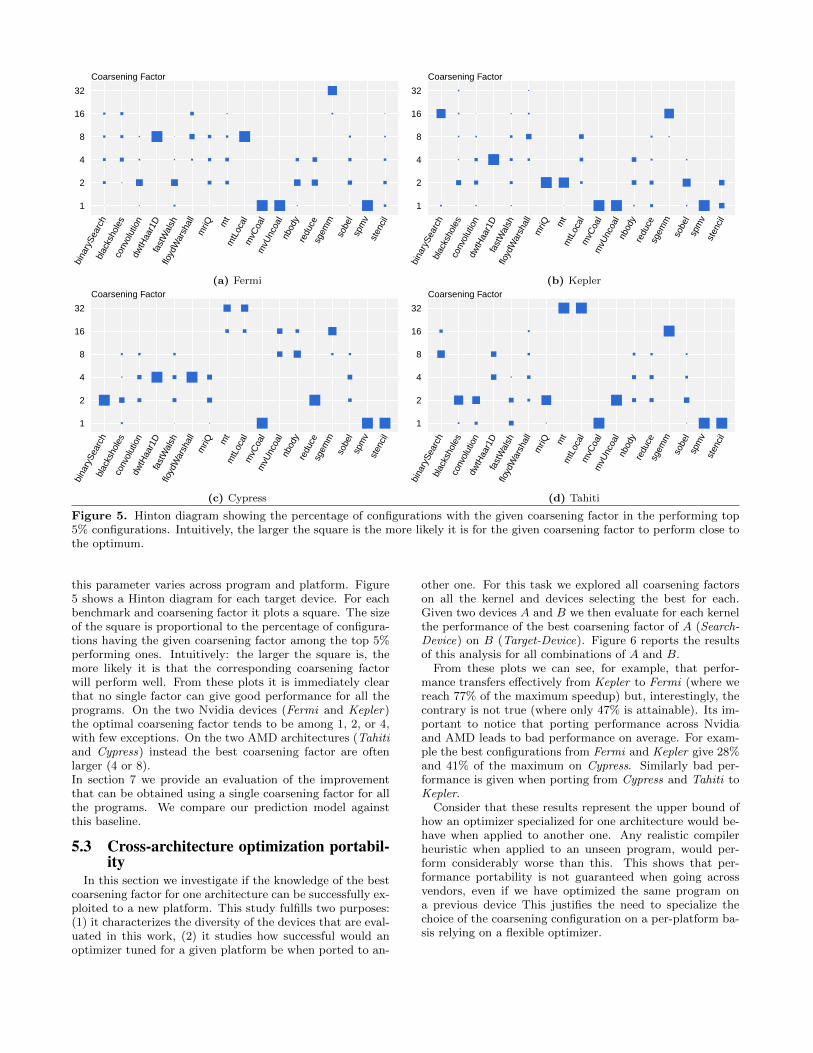
Figure 5. Hinton diagram showing the percentage of configurations with the given coarsening factor in the performing top5% configurations. Intuitively, the larger the square is the more likely it is for the given coarsening factor to perform close tothe optimum.
this parameter varies across program and platform. Figure5 shows a Hinton diagram for each target device. For eachbenchmark and coarsening factor it plots a square. The sizeof the square is proportional to the percentage of configura-tions having the given coarsening factor among the top 5%performing ones. Intuitively: the larger the square is, themore likely it is that the corresponding coarsening factorwill perform well. From these plots it is immediately clearthat no single factor can give good performance for all theprograms. On the two Nvidia devices (Fermi and Kepler)the optimal coarsening factor tends to be among 1, 2, or 4,with few exceptions. On the two AMD architectures (Tahitiand Cypress) instead the best coarsening factor are oftenlarger (4 or 8).In section 7 we provide an evaluation of the improvementthat can be obtained using a single coarsening factor for allthe programs. We compare our prediction model againstthis baseline.
5.3 Cross-architecture optimization portabil-ity
In this section we investigate if the knowledge of the bestcoarsening factor for one architecture can be successfully ex-ploited to a new platform. This study fulfills two purposes:(1) it characterizes the diversity of the devices that are eval-uated in this work, (2) it studies how successful would anoptimizer tuned for a given platform be when ported to an-
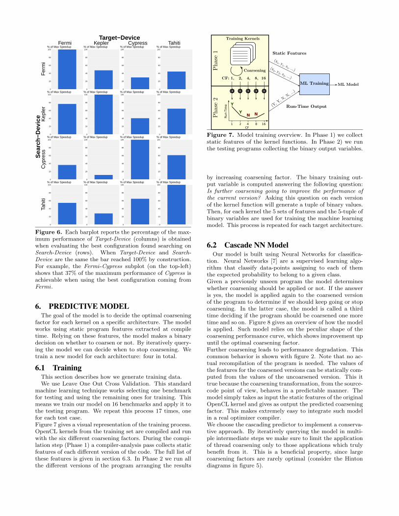
other one. For this task we explored all coarsening factorson all the kernel and devices selecting the best for each.Given two devices A and B we then evaluate for each kernelthe performance of the best coarsening factor of A (Search-Device) on B (Target-Device). Figure 6 reports the resultsof this analysis for all combinations of A and B.
From these plots we can see, for example, that perfor-mance transfers effectively from Kepler to Fermi (where wereach 77% of the maximum speedup) but, interestingly, thecontrary is not true (where only 47% is attainable). Its im-portant to notice that porting performance across Nvidiaand AMD leads to bad performance on average. For exam-ple the best configurations from Fermi and Kepler give 28%and 41% of the maximum on Cypress. Similarly bad per-formance is given when porting from Cypress and Tahiti toKepler.
Consider that these results represent the upper bound ofhow an optimizer specialized for one architecture would be-have when applied to another one. Any realistic compilerheuristic when applied to an unseen program, would per-form considerably worse than this. This shows that per-formance portability is not guaranteed when going acrossvendors, even if we have optimized the same program ona previous device This justifies the need to specialize thechoice of the coarsening configuration on a per-platform ba-sis relying on a flexible optimizer.
0
20
40
60
80
100
% of Max Speedup
0
20
40
60
80
100
% of Max Speedup
0
20
40
60
80
100
% of Max Speedup
0
20
40
60
80
100
% of Max Speedup
0
20
40
60
80
100
% of Max Speedup
0
20
40
60
80
100
% of Max Speedup
0
20
40
60
80
100
% of Max Speedup
0
20
40
60
80
100
% of Max Speedup
0
20
40
60
80
100
% of Max Speedup
0
20
40
60
80
100
% of Max Speedup
0
20
40
60
80
100
% of Max Speedup
0
20
40
60
80
100
% of Max Speedup
0
20
40
60
80
100
% of Max Speedup
0
20
40
60
80
100
% of Max Speedup
0
20
40
60
80
100
% of Max Speedup
0
20
40
60
80
100
% of Max Speedup
Tahi
tiC
ypre
ssK
eple
rF
erm
iFermi Kepler Cypress Tahiti
Sea
rch−
Dev
ice
Target−Device
Figure 6. Each barplot reports the percentage of the max-imum performance of Target-Device (columns) is obtainedwhen evaluating the best configuration found searching onSearch-Device (rows). When Target-Device and Search-Device are the same the bar reached 100% by construction.For example, the Fermi-Cypress subplot (on the top-left)shows that 37% of the maximum performance of Cypress isachievable when using the best configuration coming fromFermi .
6. PREDICTIVE MODELThe goal of the model is to decide the optimal coarsening
factor for each kernel on a specific architecture. The modelworks using static program features extracted at compiletime. Relying on these features, the model makes a binarydecision on whether to coarsen or not. By iteratively query-ing the model we can decide when to stop coarsening. Wetrain a new model for each architecture: four in total.
6.1 TrainingThis section describes how we generate training data.We use Leave One Out Cross Validation. This standard
machine learning technique works selecting one benchmarkfor testing and using the remaining ones for training. Thismeans we train our model on 16 benchmarks and apply it tothe testing program. We repeat this process 17 times, onefor each test case.Figure 7 gives a visual representation of the training process.OpenCL kernels from the training set are compiled and runwith the six different coarsening factors. During the compi-lation step (Phase 1) a compiler-analysis pass collects staticfeatures of each different version of the code. The full list ofthese features is given in section 6.3. In Phase 2 we run allthe different versions of the program arranging the results
Static Features
(Y, Y, N
, N, ...
)
Run-Time Output
ML Training ML ModelCF: 1, 2, 4, 8, 16
Training Kernels
1 2 4 8 16
Y
YN N
(x2, y2 , z2 , ...)
(x1 , y1 , z1 , ...)CoarseningPhas
e 1
Phas
e 2
Run-T
ime
CF
Figure 7. Model training overview. In Phase 1) we collectstatic features of the kernel functions. In Phase 2) we runthe testing programs collecting the binary output variables.
by increasing coarsening factor. The binary training out-put variable is computed answering the following question:Is further coarsening going to improve the performance ofthe current version? Asking this question on each versionof the kernel function will generate a tuple of binary values.Then, for each kernel the 5 sets of features and the 5-tuple ofbinary variables are used for training the machine learningmodel. This process is repeated for each target architecture.
6.2 Cascade NN ModelOur model is built using Neural Networks for classifica-
tion. Neural Networks [7] are a supervised learning algo-rithm that classify data-points assigning to each of themthe expected probability to belong to a given class.Given a previously unseen program the model determineswhether coarsening should be applied or not. If the answeris yes, the model is applied again to the coarsened versionof the program to determine if we should keep going or stopcoarsening. In the latter case, the model is called a thirdtime deciding if the program should be coarsened one moretime and so on. Figure 8 gives an overview of how the modelis applied. Such model relies on the peculiar shape of thecoarsening performance curve, which shows improvement upuntil the optimal coarsening factor.Further coarsening leads to performance degradation. Thiscommon behavior is shown with figure 2. Note that no ac-tual recompilation of the program is needed. The values ofthe features for the coarsened versions can be statically com-puted from the values of the uncoarsened version. This ittrue because the coarsening transformation, from the source-code point of view, behaves in a predictable manner. Themodel simply takes as input the static features of the originalOpenCL kernel and gives as output the predicted coarseningfactor. This makes extremely easy to integrate such modelin a real optimizer compiler.We choose the cascading predictor to implement a conserva-tive approach. By iteratively querying the model in multi-ple intermediate steps we make sure to limit the applicationof thread coarsening only to those applications which trulybenefit from it. This is a beneficial property, since largecoarsening factors are rarely optimal (consider the Hintondiagrams in figure 5).

NNmodel
Coarsening ?
YesNo
Coarsening ?
YesNo
Coarsening ?
No
NNmodel
NNmodel
...
Static Code Features
Predicted Coarsening Factor
Kernel (CF1)
Cascade NN model
Kernel (CF2)
Features
Kernel (CF4)
Features
Figure 8. High-level view the use of our Neural Networkcascade model. Static source code features of the programare extracted from the original kernel code and fed into themodel which decides whether to coarsen or not. If yes, newfeatures are computed and the model is queried again. Froma high level point of view the model simply computes thebest coarsening factor from static program characteristics.At the end of the process the program is compiled using thepredicted factor.
6.3 Program FeaturesThis section describes the static feature selection process.
The model is based exclusively on static characteristics ofthe target OpenCL kernel function. These characteristics,called features, are extracted using a function pass work-ing on the LLVM intermediate representation. Note that,since our goal is to develop a portable optimizer, we don’tuse any architecture-specific feature. We apply our func-tion analysis at the LLVM-bitcode level because this is thelowest level of abstraction that is portable across architec-tures. In particular, we do not collect any information afterinstruction scheduling or register allocation, since these aretarget-specific phases. We first describe the candidate fea-tures. This is followed by the process used to reduce theseto a smaller useful subset.
6.3.1 Candidate FeatureThe full list of candidate features is given in table 3. We
selected these based on the results of previous work [21];where we analyzed which hardware performance countersare affected by the coarsening transformation. These arethe number of executed branches, memory utilization (interms of load and cache utilization) and instruction levelparallelism (ILP). We approximate these dynamic countersusing static code characteristics counterparts, such as the to-
Feature Name Description
BasicBlocks Number of Basic BlocksBranches Number of BranchesDivInsts Number of Divergent Instruc-
tionsDivRegionInsts Number of Instructions in Diver-
gent RegionsDivRegionInstsRatio Ratio between the Number of in-
structions inside Divergent Re-gions and the Total number ofinstructions
DivRegions Number of Divergent RegionsTotInsts Number of InstructionsFPInsts Number of Floating point In-
structionsILP Average ILP per Basic BlockInt/FP Inst Ratio Ration between Integer and
Floating Point InstructionsIntInsts Number of Integer InstructionsMathFunctions Number of Math Builtin Func-
tionsMLP Average MLP per Basic BlockLoads Number of LoadsStores Number of StoresUniformLoads Number of Loads that do not de-
pend on the Coarsening Direc-tion
Barriers Number of Barriers
Table 3. Candidate static features used by the machinelearning model.
tal number of kernel instructions, static number of branchesand divergent regions and static ILP. There are 17 candidatestatic features that approximate the six most important dy-namic counters.
Absolute Features.Divergent control flow has a strong impact on performance
for graphics processors because it forces the serialization ofinstructions that would normally be executed concurrentlyon the different lanes of a warp [1]. The degree of a kernelthread divergence is measured using the results of divergenceanalysis. We count the total number of divergent instruc-tions (instructions that depend on the thread-id, i.e., theposition of the work-item in the NDRange space), the totalnumber of divergent regions (CFG regions controlled by adivergent branch) and their relative size with respect to theoverall number of instructions in the kernel. Other countersrelated to the complexity of the control flow of the kernelare the total number of blocks. Finally we also compute theaverage per-block theoretical ILP and Memory Level Paral-lelism (MLP) at the LLVM instruction level. To computethe static ILP and MLP we followed the methodology pre-sented in prior work [27].
Relative Features.As described in section 2.2 the effects of thread coarsen-
ing on the shape of the code are highly predictable. Thanksto this property we can statically compute the value thatfeatures will assume after the application of the coarsen-ing transformation. This information is used during train-ing and prediction. In particular, for each feature, we alsocalculate its relative increase caused by thread coarsening.This value is computed according to the following formula:
Delta TotInsts Delta IntInsts Delta Loads Delta Stores Delta DivInsts
Delta Branches Delta BasicBlocks Delta ILP Delta MLP Delta DivRegions Delta DivRegionInsts
FPInsts DivInsts MathFunctions FP/Int Inst Ratio
TotInsts Branches IntInsts Loads BasicBlocks
Stores Barriers UniformLoads DivRegionInsts DivRegionInstsRatio Delta UniformLoads Delta DivRegionInstsRatio
Delta FPInsts Delta MathFunctions Delta FP/Int Inst Ratio
ILP MLP DivRegions
1. Delta Instructions2. Delta Divergence3. Arithmetic Intensity
4. Instructions
5. Divergence6. Delta Arithmetic Intensity
7. Instruction Parallelism7) Instruction Parallelism
6) Delta Arithmetic Intensity
5) Divergence
4) Instructions
3) Arithmetic Intensity
2) Delta Divergence
1) Delta Instructions
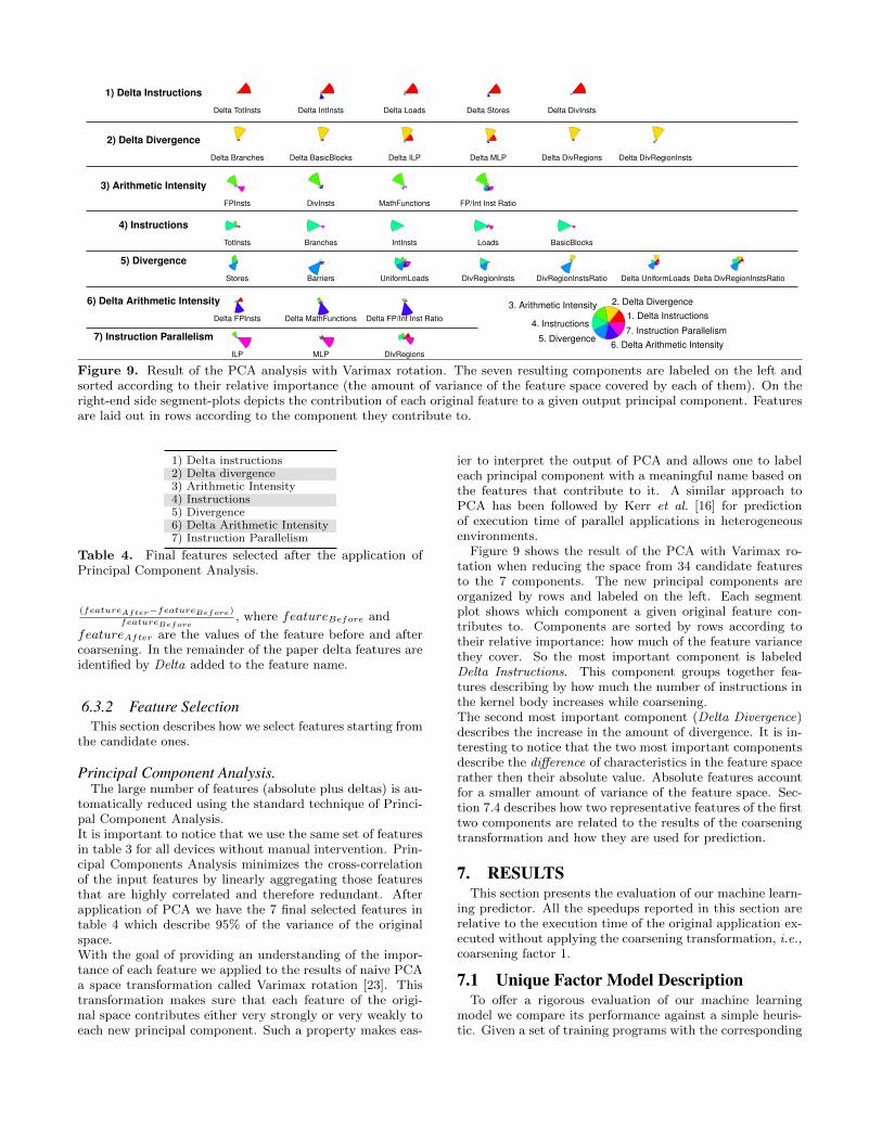
Figure 9. Result of the PCA analysis with Varimax rotation. The seven resulting components are labeled on the left andsorted according to their relative importance (the amount of variance of the feature space covered by each of them). On theright-end side segment-plots depicts the contribution of each original feature to a given output principal component. Featuresare laid out in rows according to the component they contribute to.
1) Delta instructions2) Delta divergence3) Arithmetic Intensity4) Instructions5) Divergence6) Delta Arithmetic Intensity7) Instruction Parallelism
Table 4. Final features selected after the application ofPrincipal Component Analysis.
(featureAfter−featureBefore)
featureBefore, where featureBefore and
featureAfter are the values of the feature before and aftercoarsening. In the remainder of the paper delta features areidentified by Delta added to the feature name.
6.3.2 Feature SelectionThis section describes how we select features starting from
the candidate ones.
Principal Component Analysis.The large number of features (absolute plus deltas) is au-
tomatically reduced using the standard technique of Princi-pal Component Analysis.It is important to notice that we use the same set of featuresin table 3 for all devices without manual intervention. Prin-cipal Components Analysis minimizes the cross-correlationof the input features by linearly aggregating those featuresthat are highly correlated and therefore redundant. Afterapplication of PCA we have the 7 final selected features intable 4 which describe 95% of the variance of the originalspace.With the goal of providing an understanding of the impor-tance of each feature we applied to the results of naive PCAa space transformation called Varimax rotation [23]. Thistransformation makes sure that each feature of the origi-nal space contributes either very strongly or very weakly toeach new principal component. Such a property makes eas-
ier to interpret the output of PCA and allows one to labeleach principal component with a meaningful name based onthe features that contribute to it. A similar approach toPCA has been followed by Kerr et al. [16] for predictionof execution time of parallel applications in heterogeneousenvironments.
Figure 9 shows the result of the PCA with Varimax ro-tation when reducing the space from 34 candidate featuresto the 7 components. The new principal components areorganized by rows and labeled on the left. Each segmentplot shows which component a given original feature con-tributes to. Components are sorted by rows according totheir relative importance: how much of the feature variancethey cover. So the most important component is labeledDelta Instructions. This component groups together fea-tures describing by how much the number of instructions inthe kernel body increases while coarsening.The second most important component (Delta Divergence)describes the increase in the amount of divergence. It is in-teresting to notice that the two most important componentsdescribe the difference of characteristics in the feature spacerather then their absolute value. Absolute features accountfor a smaller amount of variance of the feature space. Sec-tion 7.4 describes how two representative features of the firsttwo components are related to the results of the coarseningtransformation and how they are used for prediction.
7. RESULTSThis section presents the evaluation of our machine learn-
ing predictor. All the speedups reported in this section arerelative to the execution time of the original application ex-ecuted without applying the coarsening transformation, i.e.,coarsening factor 1.
7.1 Unique Factor Model DescriptionTo offer a rigorous evaluation of our machine learning
model we compare its performance against a simple heuris-tic. Given a set of training programs with the corresponding
Max SpeedupNN ModelUnique Model Speedup
0
0.5
1
1.5
2
2.5
bina
rySe
arch
bl
acks
hole
s
conv
olut
ion
dw
tHaa
r1D
fa
stW
alsh
flo
ydW
arsh
all
mriQ
mt
mtL
ocal
m
vCoa
l m
vUnc
oal
nbod
y
redu
ce
sgem
m
sobe
l sp
mv
st
enci
l ge
omea
n
Speedup 2.88−3.95
(a) Fermi
0
0.5
1
1.5
2
2.5
bina
rySe
arch
bl
acks
hole
s
conv
olut
ion
dw
tHaa
r1D
fa
stW
alsh
flo
ydW
arsh
all
mriQ
mt
mtL
ocal
m
vCoa
l m
vUnc
oal
nbod
y
redu
ce
sgem
m
sobe
l sp
mv
st
enci
l ge
omea
n
Speedup
(b) Kepler
0
0.5
1
1.5
2
2.5
bina
rySe
arch
bl
acks
hole
s
conv
olut
ion
dw
tHaa
r1D
fa
stW
alsh
flo
ydW
arsh
all
mriQ
mt
mtL
ocal
m
vCoa
l m
vUnc
oal
nbod
y
redu
ce
sgem
m
sobe
l sp
mv
st
enci
l ge
omea
n
Speedup 3.21 3.24 3.78
(c) Cypress
0
0.5
1
1.5
2
2.5
binarySearch
blacksholes
convolution
dwtHaar1D
fastWalsh
floydWarshall
mriQ mt
mtLocal
mvCoal
mvUncoal
nbody
reduce
sgemm
sobel
spmv
stencil
geomean
Speedup 3.4 2.82 5.15−5.15−12.01
(d) Tahiti
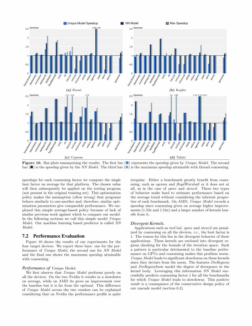
Figure 10. Bar-plots summarizing the results. The first bar (�) represents the speedup given by Unique Model. The secondbar (�) is the speedup given by the NN Model. The third bar (�) is the maximum speedup attainable with thread coarsening.
speedups for each coarsening factor we compute the singlebest factor on average for that platform. The chosen valuewill then subsequently be applied on the testing program(not present in the original training set). This optimizationpolicy makes the assumption (often wrong) that programsbehave similarly to one-another and, therefore, similar opti-mization parameters give comparable performance. We em-ployed this simple average-based policy because of lack ofsimilar previous work against which to compare our model.In the following sections we call this simple model UniqueModel. Our machine learning based predictor is called NNModel.
7.2 Performance EvaluationFigure 10 shows the results of our experiments for the
four target devices. We report three bars: one for the per-formance of Unique Model, the second one for NN Modeland the final one shows the maximum speedup attainablewith coarsening.
Performance of Unique Model.We first observe that Unique Model performs poorly on
all the devices. On the two Nvidia it results in a slowdownon average, while on AMD its gives an improvement overthe baseline but it is far from the optimal. This differenceof Unique Model across the two vendors can be explainedconsidering that on Nvidia the performance profile is quite
irregular. Either a benchmark greatly benefit from coars-ening, such as sgemm and floydWarshall or it does not atall, as in the case of spmv and stencil . These two typesof behavior make hard to estimate performance based onthe average trend without considering the inherent proper-ties of each benchmark. On AMD, Unique Model records aspeedup since coarsening given on average higher improve-ments (1.53x and 1.54x) and a larger number of kernels ben-efit from it.
Divergent Kernels.Applications such as mvCoal , spmv and stencil are penal-
ized by coarsening on all the devices, i.e., the best factor is1. The reason for this lies in the divergent behavior of theseapplications. These kernels are enclosed into divergent re-gions checking for the bounds of the iteration space. Sucha pattern is particular detrimental to the baseline perfor-mance on GPUs and coarsening makes this problem worse.Unique Model leads to significant slowdowns on these kernelssince they deviate from the norm. The features DivRegionsand DivRegionInsts model the degree of divergence in thekernel body. Leveraging this information NN Model suc-cessfully predicts coarsening factor 1 for all the benchmarksfor which Unique Model leads to slowdowns. This positiveresult is a consequence of the conservative design policy ofour cascade model (section 6.2).
Binary output in Feature Space
● ● ●
●●●
●
● ● ● ●● ●● ● ●● ●● ● ●● ● ●● ●
● ●
●●
●
●
●● ●
0.5 0.6 0.7 0.8 0.9 1
0
0.2
0.4
0.6
0.8
1
Delta TotInsts
Del
ta D
ivR
egio
ns
Thread Coarsening Effective
Thread Coarsening NOT Effective
Thread Coarsening NOT Effective
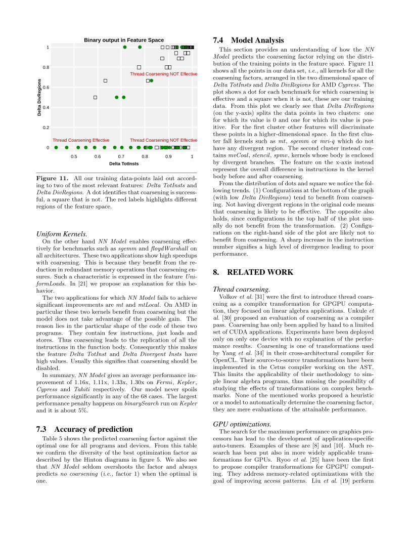
Figure 11. All our training data-points laid out accord-ing to two of the most relevant features: Delta TotInsts andDelta DivRegions. A dot identifies that coarsening is success-ful, a square that is not. The red labels highlights differentregions of the feature space.
Uniform Kernels.On the other hand NN Model enables coarsening effec-
tively for benchmarks such as sgemm and floydWarshall onall architectures. These two applications show high speedupswith coarsening. This is because they benefit from the re-duction in redundant memory operations that coarsening en-sures. Such a characteristic is expressed in the feature Uni-formLoads. In [21] we propose an explanation for this be-havior.
The two applications for which NN Model fails to achievesignificant improvements are mt and mtLocal . On AMD inparticular these two kernels benefit from coarsening but themodel does not take advantage of the possible gain. Thereason lies in the particular shape of the code of these twoprograms. They contain few instructions, just loads andstores. Thus coarsening leads to the replication of all theinstructions in the function body. Consequently this makesthe feature Delta TotInst and Delta Divergent Insts havehigh values. Usually this signifies that coarsening should bedisabled.
In summary, NN Model gives an average performance im-provement of 1.16x, 1.11x, 1.33x, 1.30x on Fermi , Kepler ,Cypress and Tahiti respectively. Our model never spoilsperformance significantly in any of the 68 cases. The largestperformance penalty happens on binarySearch run on Keplerand it is about 5%.
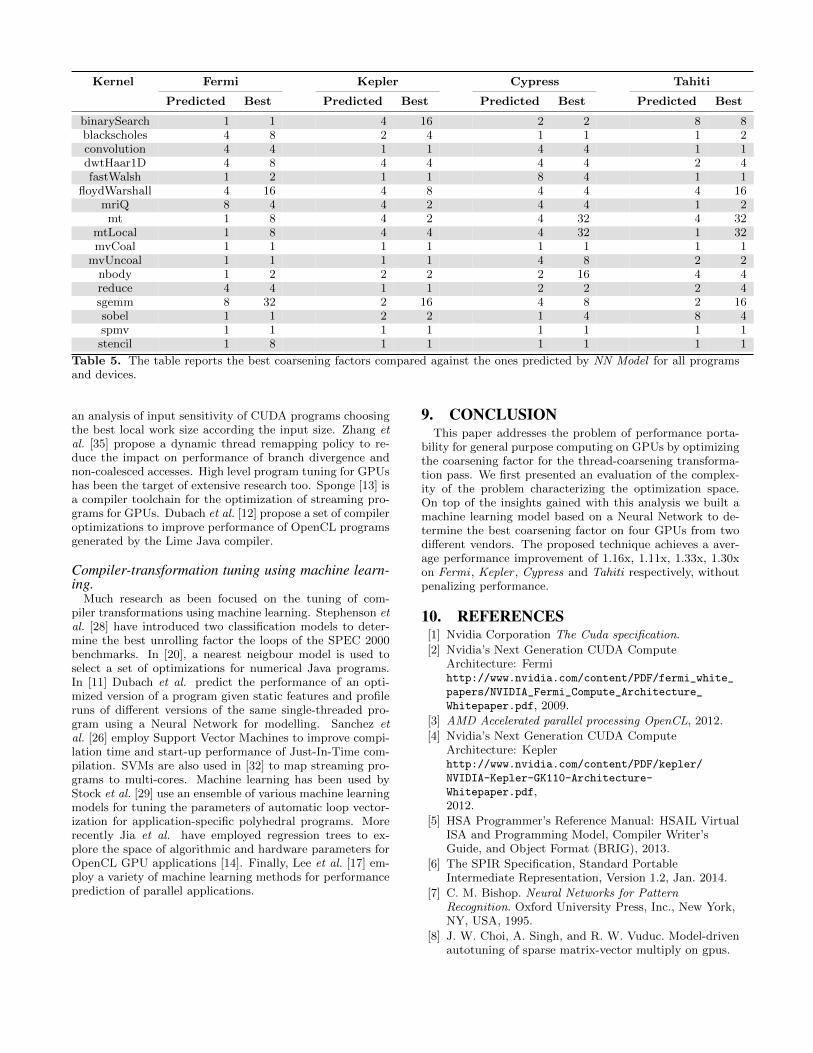
7.3 Accuracy of predictionTable 5 shows the predicted coarsening factor against the
optimal one for all programs and devices. From this tablewe confirm the diversity of the best optimization factor asdescribed by the Hinton diagrams in figure 5. We also seethat NN Model seldom overshoots the factor and alwayspredicts no coarsening (i.e., factor 1) when the optimal isone.
7.4 Model AnalysisThis section provides an understanding of how the NN
Model predicts the coarsening factor relying on the distri-bution of the training points in the feature space. Figure 11shows all the points in our data set, i.e., all kernels for all thecoarsening factors, arranged in the two dimensional space ofDelta TotInsts and Delta DivRegions for AMD Cypress. Theplot shows a dot for each benchmark for which coarsening iseffective and a square when it is not, these are our trainingdata. From this plot we clearly see that Delta DivRegions(on the y-axis) splits the data points in two clusters: onefor which its value is 0 and one for which its value is pos-itive. For the first cluster other features will discriminatethese points in a higher-dimensional space. In the first clus-ter fall kernels such as mt , sgemm or mri-q which do nothave any divergent region. The second cluster instead con-tains mvCoal , stencil , spmv , kernels whose body is enclosedby divergent branches. The feature on the x-axis insteadrepresent the overall difference in instructions in the kernelbody before and after coarsening.
From the distribution of dots and square we notice the fol-lowing trends. (1) Configurations at the bottom of the graph(with low Delta DivRegions) tend to benefit from coarsen-ing. Not having divergent regions in the original code meansthat coarsening is likely to be effective. The opposite alsoholds, since configurations in the top half of the plot usu-ally do not benefit from the transformation. (2) Configu-rations on the right-hand side of the plot are likely not tobenefit from coarsening. A sharp increase in the instructionnumber signifies a high level of divergence leading to poorperformance.
8. RELATED WORK
Thread coarsening.Volkov et al. [31] were the first to introduce thread coars-
ening as a compiler transformation for GPGPU computa-tion, they focused on linear algebra applications. Unkule etal. [30] proposed an evaluation of coarsening as a compilerpass. Coarsening has only been applied by hand to a limitedset of CUDA applications. Experiments have been deployedonly on only one device with no explanation of the perfor-mance results. Coarsening is one of transformations usedby Yang et al. [34] in their cross-architectural compiler forOpenCL. Their source-to-source transformations have beenimplemented in the Cetus compiler working on the AST.This limits the applicability of their methodology to sim-ple linear algebra programs, thus missing the possibility ofstudying the effects of transformations on complex bench-marks. None of the mentioned works proposed a heuristicor a model to automatically determine the coarsening factor,they are mere evaluations of the attainable performance.
GPU optimizations.The search for the maximum performance on graphics pro-
cessors has lead to the development of application-specificauto-tuners. Examples of these are [8] and [10]. Much re-search has been put also in more widely applicable trans-formations for GPUs. Ryoo et al. [25] have been the firstto propose compiler transformations for GPGPU comput-ing. They address memory-related optimizations with thegoal of improving access patterns. Liu et al. [19] perform
Kernel Fermi Kepler Cypress Tahiti
Predicted Best Predicted Best Predicted Best Predicted Best
binarySearch 1 1 4 16 2 2 8 8blackscholes 4 8 2 4 1 1 1 2convolution 4 4 1 1 4 4 1 1dwtHaar1D 4 8 4 4 4 4 2 4fastWalsh 1 2 1 1 8 4 1 1
floydWarshall 4 16 4 8 4 4 4 16mriQ 8 4 4 2 4 4 1 2mt 1 8 4 2 4 32 4 32
mtLocal 1 8 4 4 4 32 1 32mvCoal 1 1 1 1 1 1 1 1
mvUncoal 1 1 1 1 4 8 2 2nbody 1 2 2 2 2 16 4 4reduce 4 4 1 1 2 2 2 4sgemm 8 32 2 16 4 8 2 16sobel 1 1 2 2 1 4 8 4spmv 1 1 1 1 1 1 1 1stencil 1 8 1 1 1 1 1 1
Table 5. The table reports the best coarsening factors compared against the ones predicted by NN Model for all programsand devices.
an analysis of input sensitivity of CUDA programs choosingthe best local work size according the input size. Zhang etal. [35] propose a dynamic thread remapping policy to re-duce the impact on performance of branch divergence andnon-coalesced accesses. High level program tuning for GPUshas been the target of extensive research too. Sponge [13] isa compiler toolchain for the optimization of streaming pro-grams for GPUs. Dubach et al. [12] propose a set of compileroptimizations to improve performance of OpenCL programsgenerated by the Lime Java compiler.
Compiler-transformation tuning using machine learn-ing.
Much research as been focused on the tuning of com-piler transformations using machine learning. Stephenson etal. [28] have introduced two classification models to deter-mine the best unrolling factor the loops of the SPEC 2000benchmarks. In [20], a nearest neigbour model is used toselect a set of optimizations for numerical Java programs.In [11] Dubach et al. predict the performance of an opti-mized version of a program given static features and profileruns of different versions of the same single-threaded pro-gram using a Neural Network for modelling. Sanchez etal. [26] employ Support Vector Machines to improve compi-lation time and start-up performance of Just-In-Time com-pilation. SVMs are also used in [32] to map streaming pro-grams to multi-cores. Machine learning has been used byStock et al. [29] use an ensemble of various machine learningmodels for tuning the parameters of automatic loop vector-ization for application-specific polyhedral programs. Morerecently Jia et al. have employed regression trees to ex-plore the space of algorithmic and hardware parameters forOpenCL GPU applications [14]. Finally, Lee et al. [17] em-ploy a variety of machine learning methods for performanceprediction of parallel applications.
9. CONCLUSIONThis paper addresses the problem of performance porta-
bility for general purpose computing on GPUs by optimizingthe coarsening factor for the thread-coarsening transforma-tion pass. We first presented an evaluation of the complex-ity of the problem characterizing the optimization space.On top of the insights gained with this analysis we built amachine learning model based on a Neural Network to de-termine the best coarsening factor on four GPUs from twodifferent vendors. The proposed technique achieves a aver-age performance improvement of 1.16x, 1.11x, 1.33x, 1.30xon Fermi , Kepler , Cypress and Tahiti respectively, withoutpenalizing performance.
10. REFERENCES[1] Nvidia Corporation The Cuda specification.
[2] Nvidia’s Next Generation CUDA ComputeArchitecture: Fermihttp://www.nvidia.com/content/PDF/fermi_white_
papers/NVIDIA_Fermi_Compute_Architecture_
Whitepaper.pdf, 2009.
[3] AMD Accelerated parallel processing OpenCL, 2012.
[4] Nvidia’s Next Generation CUDA ComputeArchitecture: Keplerhttp://www.nvidia.com/content/PDF/kepler/
NVIDIA-Kepler-GK110-Architecture-
Whitepaper.pdf,2012.
[5] HSA Programmer’s Reference Manual: HSAIL VirtualISA and Programming Model, Compiler Writer’sGuide, and Object Format (BRIG), 2013.
[6] The SPIR Specification, Standard PortableIntermediate Representation, Version 1.2, Jan. 2014.
[7] C. M. Bishop. Neural Networks for PatternRecognition. Oxford University Press, Inc., New York,NY, USA, 1995.
[8] J. W. Choi, A. Singh, and R. W. Vuduc. Model-drivenautotuning of sparse matrix-vector multiply on gpus.
PPoPP ’10, pages 115–126, New York, NY, USA,2010. ACM.
[9] B. Coutinho, D. Sampaio, F. Pereira, and W. Meira.Divergence analysis and optimizations. PACT, pages320 –329, oct. 2011.
[10] Y. Dotsenko, S. S. Baghsorkhi, B. Lloyd, and N. K.Govindaraju. Auto-tuning of fast fourier transform ongraphics processors. SIGPLAN Not., 46(8):257–266,Feb. 2011.
[11] C. Dubach, J. Cavazos, B. Franke, G. Fursin, M. F.O’Boyle, and O. Temam. Fast compiler optimisationevaluation using code-feature based performanceprediction. CF ’07, pages 131–142, New York, NY,USA, 2007. ACM.
[12] C. Dubach, P. Cheng, R. M. Rabbah, D. F. Bacon,and S. J. Fink. Compiling a high-level language forgpus: (via language support for architectures andcompilers). In PLDI, pages 1–12, 2012.
[13] A. H. Hormati, M. Samadi, M. Woh, T. Mudge, andS. Mahlke. Sponge: portable stream programming ongraphics engines. ASPLOS ’11, pages 381–392, NewYork, NY, USA, 2011. ACM.
[14] W. Jia, K. Shaw, and M. Martonosi. Starchart:Hardware and software optimization using recursivepartitioning regression trees. PACT ’13, 2013.
[15] R. Karrenberg and S. Hack. Improving performance ofopencl on cpus. CC, pages 1–20, 2012.
[16] A. Kerr, G. Diamos, and S. Yalamanchili. Modelinggpu-cpu workloads and systems. GPGPU ’10, pages31–42, New York, NY, USA, 2010. ACM.
[17] B. C. Lee, D. M. Brooks, B. R. de Supinski,M. Schulz, K. Singh, and S. A. McKee. Methods ofinference and learning for performance modeling ofparallel applications. PPoPP ’07, pages 249–258, NewYork, NY, USA, 2007. ACM.
[18] Y. Lee, R. Krashinsky, V. Grover, S. W. Keckler, and
K. AsanoviAG. Convergence and scalarization fordata-parallel architectures, 2013.
[19] Y. Liu, E. Zhang, and X. Shen. A cross-input adaptiveframework for gpu program optimizations. IPDPS ’09,pages 1 –10, may 2009.
[20] S. Long and M. F. O’Boyle. Adptive java optimisationusing instance-based learning. ICS, pages 237–246,2004.
[21] A. Magni, C. Dubach, and M. F. O’Boyle. Alarge-scale cross-architecture evaluation ofthread-coarsening. SC ’13. ACM, 2013.
[22] A. Magni, C. Dubach, and M. F. P. O’Boyle.Exploiting gpu hardware saturation for fast compileroptimization. GPGPU-7, 2014.
[23] B. Manly. Multivariate Statistical Methods: A Primer,Third Edition. Taylor & Francis, 2004.
[24] S. Moll. Decompilation of LLVM IR, 2011.
[25] S. Ryoo, C. I. Rodrigues, S. S. Baghsorkhi, S. S.Stone, D. B. Kirk, and W.-m. W. Hwu. Optimizationprinciples and application performance evaluation of amultithreaded gpu using cuda. PPoPP ’08, pages73–82, New York, NY, USA, 2008. ACM.
[26] R. Sanchez, J. Amaral, D. Szafron, M. Pirvu, andM. Stoodley. Using machines to learn method-specificcompilation strategies. CGO ’11, pages 257 –266, april2011.
[27] J. Sim, A. Dasgupta, H. Kim, and R. Vuduc. Aperformance analysis framework for identifyingpotential benefits in gpgpu applications. PPoPP ’12,pages 11–22, New York, NY, USA, 2012. ACM.
[28] M. Stephenson and S. Amarasinghe. Predicting unrollfactors using supervised classification. CGO ’05, pages123–134, Washington, DC, USA, 2005. IEEEComputer Society.
[29] K. Stock, L.-N. Pouchet, and P. Sadayappan. Usingmachine learning to improve automatic vectorization.ACM Trans. Archit. Code Optim., 8(4):50:1–50:23,Jan. 2012.
[30] S. Unkule, C. Shaltz, and A. Qasem. Automaticrestructuring of gpu kernels for exploiting inter-threaddata locality. CC, pages 21–40, 2012.
[31] V. Volkov and J. W. Demmel. Benchmarking gpus totune dense linear algebra. SC ’08, pages 31:1–31:11,Piscataway, NJ, USA, 2008. IEEE Press.
[32] Z. Wang and M. F. O’Boyle. Partitioning streamingparallelism for multi-cores: A machine learning basedapproach. PACT, 2010.
[33] P. Xiang, Y. Yang, M. Mantor, N. Rubin, L. R. Hsu,and H. Zhou. Exploiting uniform vector instructionsfor gpgpu performance, energy efficiency, andopportunistic reliability enhancement. ICS ’13, pages433–442, New York, NY, USA, 2013. ACM.
[34] Y. Yang, P. Xiang, J. Kong, M. Mantor, and H. Zhou.A unified optimizing compiler framework for differentgpgpu architectures. TACO, 9(2):9, 2012.
[35] E. Z. Zhang, Y. Jiang, Z. Guo, K. Tian, and X. Shen.On-the-fly elimination of dynamic irregularities forgpu computing. ASPLOS ’11, pages 369–380, NewYork, NY, USA, 2011. ACM.