Automatic Sound Synthesizer

Programming: Techniques and

Applications

Matthew John Yee-King

Submitted for the degree of Doctor of Philosophy

University of Sussex

January 2011

Declaration

I hereby declare that this thesis has not been and will not be submitted in whole or in

part to another University for the award of any other degree.

Signature:

Matthew John Yee-King

iii

UNIVERSITY OF SUSSEX

Matthew John Yee-King, Doctor of Philosophy

Automatic Sound Synthesizer Programming - Techniques and Applications

Summary

The aim of this thesis is to investigate techniques for, and applications of automaticsound synthesizer programming. An automatic sound synthesizer programmer is a systemwhich removes the requirement to explicitly specify parameter settings for a sound syn-thesis algorithm from the user. Two forms of these systems are discussed in this thesis:tone matching programmers and synthesis space explorers. A tone matching programmertakes at its input a sound synthesis algorithm and a desired target sound. At its outputit produces a configuration for the sound synthesis algorithm which causes it to emit asimilar sound to the target. The techniques for achieving this that are investigated aregenetic algorithms, neural networks, hill climbers and data driven approaches. A synthe-sis space explorer provides a user with a representation of the space of possible soundsthat a synthesizer can produce and allows them to interactively explore this space. Theapplications of automatic sound synthesizer programming that are investigated includestudio tools, an autonomous musical agent and a self-reprogramming drum machine. Theresearch employs several methodologies: the development of novel software frameworksand tools, the examination of existing software at the source code and performance levelsand user trials of the tools and software. The main contributions made are: a methodfor visualisation of sound synthesis space and low dimensional control of sound synthesiz-ers; a general purpose framework for the deployment and testing of sound synthesis andoptimisation algorithms in the SuperCollider language sclang; a comparison of a varietyof optimisation techniques for sound synthesizer programming; an analysis of sound syn-thesizer error surfaces; a general purpose sound synthesizer programmer compatible withindustry standard tools; an automatic improviser which passes a loose equivalent of theTuring test for Jazz musicians, i.e. being half of a man-machine duet which was rated asone of the best sessions of 2009 on the BBC’s ’Jazz on 3’ programme.

iv

Acknowledgements

Thanks and love to Sakie, Otone and Synthesizer the dog for their unwavering support of

my creative and academic endeavours. Also to my other close family members for always

encouraging me to take my own path.

Thanks to Nick Collins for being an excellent and very accommodating supervisor.

I could not have done this without Nick! Thanks also to Chris Thornton, Christopher

Frauenberger, Phil Husbands and Adrian Thompson for their academic input along the

way.

Thanks to Finn Peters and his merry band of musicians for patiently allowing me

to turn rehearsals, recording sessions and live gigs into ad-hoc experiments and for their

valued input into my research work.

Thanks to Martin Roth for many interesting conversations and long nights program-

ming various implementations of SynthBot.

Thanks to the synthesizer programmers who were involved in the man vs. machine

trial. Note that I was the best at programming the FM synthesizer... ha!. Thanks also to

Graham ‘Gaz’/ ‘Bavin’ Gatheral and Mike Brooke for their trialling of the drum machine.

Also all of the other great musicians I have been lucky enough to work with.

Thanks to the anonymous reviewers for their comments on the papers, to the Depart-

ment of Informatics for funding for conferences and for letting me do interesting research.

Thanks to the Goldsmiths Department of Computing, especially Mark D’Inverno and

Sarah Rauchas for being very accommodating when I needed to write this thesis.

Thanks to Drew Gartland-Jones who was my original supervisor and who helped to

set me on this trajectory in the first place.

v

Abstract

The aim of this thesis is to investigate techniques for, and applications of automatic sound

synthesizer programming. An automatic sound synthesizer programmer is a system which

removes the requirement to explicitly specify parameter settings for a sound synthesis

algorithm from the user. Two forms of these systems are discussed in this thesis: tone

matching programmers and synthesis space explorers. A tone matching programmer takes

at its input a sound synthesis algorithm and a desired target sound. At its output it pro-

duces a configuration for the sound synthesis algorithm which causes it to emit a similar

sound to the target. The techniques for achieving this that are investigated are genetic

algorithms, neural networks, hill climbers and data driven approaches. A synthesis space

explorer provides a user with a representation of the space of possible sounds that a syn-

thesizer can produce and allows them to interactively explore this space. The applications

of automatic sound synthesizer programming that are investigated include studio tools,

an autonomous musical agent and a self-reprogramming drum machine. The research em-

ploys several methodologies: the development of novel software frameworks and tools, the

examination of existing software at the source code and performance levels and user trials

of the tools and software. The main contributions made are: a method for visualisation of

sound synthesis space and low dimensional control of sound synthesizers; a general purpose

framework for the deployment and testing of sound synthesis and optimisation algorithms

in the SuperCollider language sclang; a comparison of a variety of optimisation techniques

for sound synthesizer programming; an analysis of sound synthesizer error surfaces; a gen-

eral purpose sound synthesizer programmer compatible with industry standard tools; an

automatic improviser which passes a loose equivalent of the Turing test for Jazz musicians,

i.e. being half of a man-machine duet which was rated as one of the best sessions of 2009

on the BBC’s ’Jazz on 3’ programme.

vi

Related Publications

Three of the chapters in this thesis are based on peer reviewed, published papers. A short

version of chapter 4 was presented as ‘SynthBot - an unsupervised software synthesizer

programmer’ at ICMC 2008 [144]. It should be noted that this paper was co-authored with

Martin Roth. However, the author was responsible for designing and carrying out the user

and technical trials reported in this thesis as well as implementing the genetic algorithm

which forms the core of the SynthBot software. Martin Roth implemented the Java based

VST host component of SynthBot and has been more involved in subsequent iterations

of the SynthBot software, which are not reported in detail in this thesis. Chapter 5 is an

extended version of a paper that was originally presented as ‘The Evolving Drum Machine’

at ECAL 2008 and later appeared as a book chapter in 2010 [143, 140]. Chapter 6 is an

extended version of a paper presented at the EvoMUSART workshop at the EvoWorkshops

conference in 2007 [142]. The software developed for the purposes of this thesis has

been used in several performances and recording sessions. Most notably, the automated

improviser appears on Finn Peters’ ‘Butterflies’ and ‘Music of the Mind’ albums and a

duet featuring Finn Peters and the algorithm was recorded for BBC Radio 3’s ‘Jazz on 3’

[94, 96, 28].

vii

Contents

List of Tables xiii

List of Figures xviii

1 Introduction 1

1.1 Research Context and Personal Motivation . . . . . . . . . . . . . . . . . . 4

1.2 Research Questions . . . . . . . . . . . . . . . . . . . . . . . . . . . . . . . . 8

1.3 Aims and Contributions . . . . . . . . . . . . . . . . . . . . . . . . . . . . . 10

1.4 Methodology . . . . . . . . . . . . . . . . . . . . . . . . . . . . . . . . . . . 12

1.4.1 Software . . . . . . . . . . . . . . . . . . . . . . . . . . . . . . . . . . 13

1.4.2 Numerical Evaluation . . . . . . . . . . . . . . . . . . . . . . . . . . 14

1.4.3 User Trials . . . . . . . . . . . . . . . . . . . . . . . . . . . . . . . . 14

1.5 Thesis Structure . . . . . . . . . . . . . . . . . . . . . . . . . . . . . . . . . 14

2 Perception and Representation of Timbre 16

2.1 The Ascending Auditory Pathway . . . . . . . . . . . . . . . . . . . . . . . 16

2.1.1 From Outer Ear to Basilar Membrane . . . . . . . . . . . . . . . . . 17

2.1.2 From Basilar Membrane to Auditory Nerve . . . . . . . . . . . . . . 17

2.1.3 From Auditory Nerve to Auditory Cortex: Information Representation 18

2.1.4 Sparse Coding of Auditory Information . . . . . . . . . . . . . . . . 19

2.2 Defining Timbre and Timbre Perception . . . . . . . . . . . . . . . . . . . . 20

2.2.1 What is Timbre? . . . . . . . . . . . . . . . . . . . . . . . . . . . . . 20

2.2.2 Inseparability of Pitch and Timbre . . . . . . . . . . . . . . . . . . . 20

2.2.3 Imagining Timbre . . . . . . . . . . . . . . . . . . . . . . . . . . . . 21

2.2.4 Listener-Based Timbre Similarity Experiments . . . . . . . . . . . . 22

2.3 The Ideal Numerical Representation of Timbre . . . . . . . . . . . . . . . . 25

2.4 The MFCC Feature . . . . . . . . . . . . . . . . . . . . . . . . . . . . . . . 26

2.4.1 Extracting MFCCs . . . . . . . . . . . . . . . . . . . . . . . . . . . . 27

viii

2.4.2 MFCCs for Music Orientated Tasks . . . . . . . . . . . . . . . . . . 30

2.4.3 Open Source MFCC Implementations . . . . . . . . . . . . . . . . . 30

2.4.4 An Implementation-level Comparison of Open Source MFCC extrac-

tors . . . . . . . . . . . . . . . . . . . . . . . . . . . . . . . . . . . . 31

2.4.5 A Performance Comparison of the MFCC Extractors . . . . . . . . . 33

2.4.6 Novel MFCC Extractor Implementation . . . . . . . . . . . . . . . . 38

2.5 Presenting Timbre Similarity: SoundExplorer . . . . . . . . . . . . . . . . . 38

2.5.1 Interaction . . . . . . . . . . . . . . . . . . . . . . . . . . . . . . . . 40

2.5.2 Graphical Output . . . . . . . . . . . . . . . . . . . . . . . . . . . . 41

2.5.3 User Experience . . . . . . . . . . . . . . . . . . . . . . . . . . . . . 44

2.6 Summary . . . . . . . . . . . . . . . . . . . . . . . . . . . . . . . . . . . . . 46

3 Searching Sound Synthesis Space 47

3.1 The Sound Synthesis Algorithms . . . . . . . . . . . . . . . . . . . . . . . . 48

3.1.1 FM Synthesis . . . . . . . . . . . . . . . . . . . . . . . . . . . . . . . 48

3.1.2 Subtractive Synthesis . . . . . . . . . . . . . . . . . . . . . . . . . . 50

3.1.3 Variable Architecture Synthesis . . . . . . . . . . . . . . . . . . . . . 52

3.2 Synthesis Feature Space Analysis . . . . . . . . . . . . . . . . . . . . . . . . 54

3.2.1 Error Surface Analysis . . . . . . . . . . . . . . . . . . . . . . . . . . 54

3.2.2 Error Surface Analysis: FM Synthesis . . . . . . . . . . . . . . . . . 56

3.2.3 Error Surface Analysis: Subtractive Synthesis . . . . . . . . . . . . . 61

3.3 The Optimisation Techniques . . . . . . . . . . . . . . . . . . . . . . . . . . 65

3.3.1 Basic Hill Climbing . . . . . . . . . . . . . . . . . . . . . . . . . . . . 65

3.3.2 Feed Forward Neural Network . . . . . . . . . . . . . . . . . . . . . . 66

3.3.3 Genetic Algorithm . . . . . . . . . . . . . . . . . . . . . . . . . . . . 69

3.3.4 Basic Data Driven ‘Nearest Neighbour’ Approach . . . . . . . . . . . 70

3.4 Results . . . . . . . . . . . . . . . . . . . . . . . . . . . . . . . . . . . . . . . 71

3.4.1 Optimiser Test Set Performance . . . . . . . . . . . . . . . . . . . . 72

3.4.2 Instrument Timbre Matching Performance . . . . . . . . . . . . . . . 75

3.4.3 Conclusion . . . . . . . . . . . . . . . . . . . . . . . . . . . . . . . . 80

4 Sound Synthesis Space Exploration as a Studio Tool: SynthBot 82

4.1 Introduction . . . . . . . . . . . . . . . . . . . . . . . . . . . . . . . . . . . . 83

4.1.1 The Difficulty of Programming Synthesizers . . . . . . . . . . . . . . 83

4.1.2 Applying Machine Learning to Synthesizer Programming . . . . . . 84

ix

4.1.3 The Need for SynthBot . . . . . . . . . . . . . . . . . . . . . . . . . 85

4.2 Implementation . . . . . . . . . . . . . . . . . . . . . . . . . . . . . . . . . . 85

4.2.1 Background Technologies . . . . . . . . . . . . . . . . . . . . . . . . 85

4.2.2 Sound Synthesis . . . . . . . . . . . . . . . . . . . . . . . . . . . . . 86

4.2.3 Automatic Parameter Search . . . . . . . . . . . . . . . . . . . . . . 86

4.3 Technical Evaluation . . . . . . . . . . . . . . . . . . . . . . . . . . . . . . . 90

4.4 Experimental Evaluation . . . . . . . . . . . . . . . . . . . . . . . . . . . . . 93

4.4.1 Software for Experimental Evaluation . . . . . . . . . . . . . . . . . 94

4.4.2 Results . . . . . . . . . . . . . . . . . . . . . . . . . . . . . . . . . . 95

4.5 Conclusion . . . . . . . . . . . . . . . . . . . . . . . . . . . . . . . . . . . . 101

4.5.1 Epilogue: The Current State of SynthBot . . . . . . . . . . . . . . . 102

5 Sound Synthesis Space Exploration in Live Performance: The Evolving

Drum Machine 103

5.1 Introduction . . . . . . . . . . . . . . . . . . . . . . . . . . . . . . . . . . . . 103

5.2 System Overview . . . . . . . . . . . . . . . . . . . . . . . . . . . . . . . . . 104

5.3 User Interface . . . . . . . . . . . . . . . . . . . . . . . . . . . . . . . . . . . 105

5.4 Sound Synthesis . . . . . . . . . . . . . . . . . . . . . . . . . . . . . . . . . 108

5.4.1 SoundExplorer Map of Sound Synthesis Space . . . . . . . . . . . . 110

5.5 Search . . . . . . . . . . . . . . . . . . . . . . . . . . . . . . . . . . . . . . . 113

5.5.1 Genetic Encoding . . . . . . . . . . . . . . . . . . . . . . . . . . . . . 113

5.5.2 Fitness Function . . . . . . . . . . . . . . . . . . . . . . . . . . . . . 114

5.5.3 Breeding Strategies . . . . . . . . . . . . . . . . . . . . . . . . . . . . 114

5.5.4 Genome Manipulation . . . . . . . . . . . . . . . . . . . . . . . . . . 114

5.6 Results: GA Performance . . . . . . . . . . . . . . . . . . . . . . . . . . . . 116

5.6.1 General Performance . . . . . . . . . . . . . . . . . . . . . . . . . . . 116

5.6.2 Algorithm Settings and Their Effect on Musical Output . . . . . . . 116

5.7 Results: User Experiences . . . . . . . . . . . . . . . . . . . . . . . . . . . . 119

5.8 Conclusion . . . . . . . . . . . . . . . . . . . . . . . . . . . . . . . . . . . . 121

6 The Timbre Matching Improviser 122

6.1 Related Work . . . . . . . . . . . . . . . . . . . . . . . . . . . . . . . . . . . 122

6.1.1 Genetic Algorithm Driven Sound Synthesis . . . . . . . . . . . . . . 123

6.2 Technical Implementation . . . . . . . . . . . . . . . . . . . . . . . . . . . . 125

6.2.1 Sound Synthesis . . . . . . . . . . . . . . . . . . . . . . . . . . . . . 125

x

6.2.2 Search . . . . . . . . . . . . . . . . . . . . . . . . . . . . . . . . . . . 128

6.2.3 Listening . . . . . . . . . . . . . . . . . . . . . . . . . . . . . . . . . 129

6.2.4 Improvisation . . . . . . . . . . . . . . . . . . . . . . . . . . . . . . . 129

6.3 Analysis . . . . . . . . . . . . . . . . . . . . . . . . . . . . . . . . . . . . . . 131

6.3.1 Moving Target Search . . . . . . . . . . . . . . . . . . . . . . . . . . 131

6.3.2 User Feedback . . . . . . . . . . . . . . . . . . . . . . . . . . . . . . 132

6.4 Conclusion . . . . . . . . . . . . . . . . . . . . . . . . . . . . . . . . . . . . 135

7 Conclusion 137

7.1 Research Questions . . . . . . . . . . . . . . . . . . . . . . . . . . . . . . . . 137

7.2 Contributions . . . . . . . . . . . . . . . . . . . . . . . . . . . . . . . . . . . 141

7.3 Future Work . . . . . . . . . . . . . . . . . . . . . . . . . . . . . . . . . . . 142

7.3.1 Chapter 2 . . . . . . . . . . . . . . . . . . . . . . . . . . . . . . . . . 143

7.3.2 Chapter 3 . . . . . . . . . . . . . . . . . . . . . . . . . . . . . . . . . 143

7.3.3 Chapter 4 . . . . . . . . . . . . . . . . . . . . . . . . . . . . . . . . . 144

7.3.4 Chapter 5 . . . . . . . . . . . . . . . . . . . . . . . . . . . . . . . . . 144

7.3.5 Chapter 6 . . . . . . . . . . . . . . . . . . . . . . . . . . . . . . . . . 144

7.4 Summary . . . . . . . . . . . . . . . . . . . . . . . . . . . . . . . . . . . . . 145

Bibliography 147

A Audio CD Track Listing 160

xi

List of Tables

2.1 Sounds that are both far away and equidistant from a reference sound in

Beads MFCC feature space, along with the distances between the sounds

in Beads MFCC feature space. . . . . . . . . . . . . . . . . . . . . . . . . . 35

2.2 Pearson’s correlations between the distance matrices for each MFCC ex-

tractor and the reference matrix. . . . . . . . . . . . . . . . . . . . . . . . . 37

2.3 This table shows the indices used for the synth vs. real instrument plots in

figures 2.8 and 2.10. . . . . . . . . . . . . . . . . . . . . . . . . . . . . . . . 41

3.1 The table on the left shows the FM7 oscillator parameter matrix which

defines frequency, phase and amplitude for the six sine oscillators. The

table on the right shows the parameters from the FM7 phase modulation

matrix which defines modulation indices from every oscillator to itself and

all other oscillators. E.g. m1..6 define the modulation from oscillators 1-6

to oscillator 1. . . . . . . . . . . . . . . . . . . . . . . . . . . . . . . . . . . 49

3.2 This table lists the parameters for the complex FM synthesis algorithm. The

first six parameters are duplicated for each of the three active oscillators. . 51

3.3 This table lists the parameters for the basic subtractive synthesis algorithm. 51

3.4 This table lists the parameters for the complex subtractive synthesis algo-

rithm. Note that f is the base frequency. . . . . . . . . . . . . . . . . . . . 53

3.5 This table shows the parameters for the variable architecture synthesis al-

gorithm. f is the base frequency. . . . . . . . . . . . . . . . . . . . . . . . . 54

3.6 The best neural network settings found for each synthesizer. . . . . . . . . . 67

xii

3.7 This table shows the mean performance per optimiser per synthesizer across

the 50 sounds in each synthesizer’s test set. The score is the reciprocal of

the distance between the error and the target normalised by the feature

vector size. The SD% column is the standard deviation as a percentage of

the mean and the final column is the non-normalised error, comparable to

the values in the error surface plots. . . . . . . . . . . . . . . . . . . . . . . 73

3.8 This table shows the errors achieved by repeated runs of the GA against the

targets from the test set for which it achieved the best, worst and middle

results. . . . . . . . . . . . . . . . . . . . . . . . . . . . . . . . . . . . . . . . 75

3.9 This table shows the mean performance per optimiser, per synthesizer across

the 20 real instrument sounds. The data is sorted by score so the best

performing synthesizer/ optimiser combinations appear at the top. . . . . . 76

3.10 This table shows the best matches achieved for each of the 20 real instru-

ment sounds. . . . . . . . . . . . . . . . . . . . . . . . . . . . . . . . . . . . 77

3.11 This table compares the timbre matching performance of the data driven

nearest neighbour search with 100,000 and 200,000 point data sets from the

complex FM synthesizer. The final column shows the reduction in error

observed with the larger data set. . . . . . . . . . . . . . . . . . . . . . . . 79

3.12 This table compares the standard GA which starts with a random popula-

tion to the hybrid GA which starts with a population derived from a data

driven search. . . . . . . . . . . . . . . . . . . . . . . . . . . . . . . . . . . 80

4.1 The parameters that are used to control the mdaDX10 synthesizer. . . . . . 87

4.2 The parameters that are used to control the mdaJX10 synthesizer, adapted

from the mdaJX10 user manual [62]. . . . . . . . . . . . . . . . . . . . . . . 88

4.3 The best results achieved by the human participants and SynthBot for each

sound. The errors are Euclidean distances in MFCC space between the

target and candidate sounds, normalised using the length of the sounds to

enable easier comparison. A lower error indicates a better match. . . . . . . 95

5.1 The parameters encoded in the genome with example values for the gen-

eration 100 sound shown in Figure 5.11. Example values rounded from 16

decimal places. . . . . . . . . . . . . . . . . . . . . . . . . . . . . . . . . . . 111

xiii

6.1 The parameters for the synthdefs used to make the additively synthesed

sounds. These parameters are derived directly from the numbers stored in

the genome . . . . . . . . . . . . . . . . . . . . . . . . . . . . . . . . . . . . 127

6.2 The parameters for the synthdefs used in the FM synthesized sounds . . . . 127

xiv

List of Figures

2.1 Different plots of human similarity judgements, derived by performing MDS

on similarity matrices. Top taken from Grey 1976 [42], middle taken from

Iverson and Krumhansl 1993 [57] and bottom taken from Halpern et al.

2004 [43]. . . . . . . . . . . . . . . . . . . . . . . . . . . . . . . . . . . . . . 24

2.2 An overview of the process of extracting an MFCC feature vector from a

time domain signal. . . . . . . . . . . . . . . . . . . . . . . . . . . . . . . . . 27

2.3 Comparison of the mel frequency scale approximated using equation 2.1 to

midi notes, based on equal temperament tuning. . . . . . . . . . . . . . . . 28

2.4 Perceptual scaling functions used for the different feature extractors. Clock-

wise from the top left: CoMIRVA, Beads, SuperCollider3 and libxtract. . . 33

2.5 Normalised distances from a reference sound to each of the other sounds.

The reference sound has index 0. The linear plot included shows the ex-

pected distance if distance in feature space correlates with distance in pa-

rameter space. . . . . . . . . . . . . . . . . . . . . . . . . . . . . . . . . . . 34

2.6 Distance matrices showing the sum squared Euclidean distance between

each of the 100 sounds for each of the MFCC extractors, along with a

reference matrix showing the normalised distance in parameter space. . . . 36

2.7 Screen shots from the SoundExplorer program, showing 5000 sounds sam-

pled at random from 4 synthesis algorithms. Note that the axes are not

labelled since they do not pertain to any specific measure other than being

the two dimensions of the MDS output. . . . . . . . . . . . . . . . . . . . . 42

2.8 Screen shots from the SoundExplorer program showing 5000 random sounds

from each synth plotted against the 20 acoustic instrument sounds. Note

that the axes are not labelled since they do not pertain to any specific

measure other than being the two dimensions of the MDS output. . . . . . 43

xv

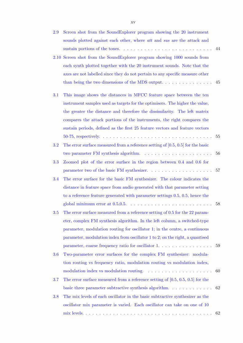
2.9 Screen shot from the SoundExplorer program showing the 20 instrument

sounds plotted against each other, where att and sus are the attack and

sustain portions of the tones. . . . . . . . . . . . . . . . . . . . . . . . . . . 44

2.10 Screen shot from the SoundExplorer program showing 1000 sounds from

each synth plotted together with the 20 instrument sounds. Note that the

axes are not labelled since they do not pertain to any specific measure other

than being the two dimensions of the MDS output. . . . . . . . . . . . . . . 45

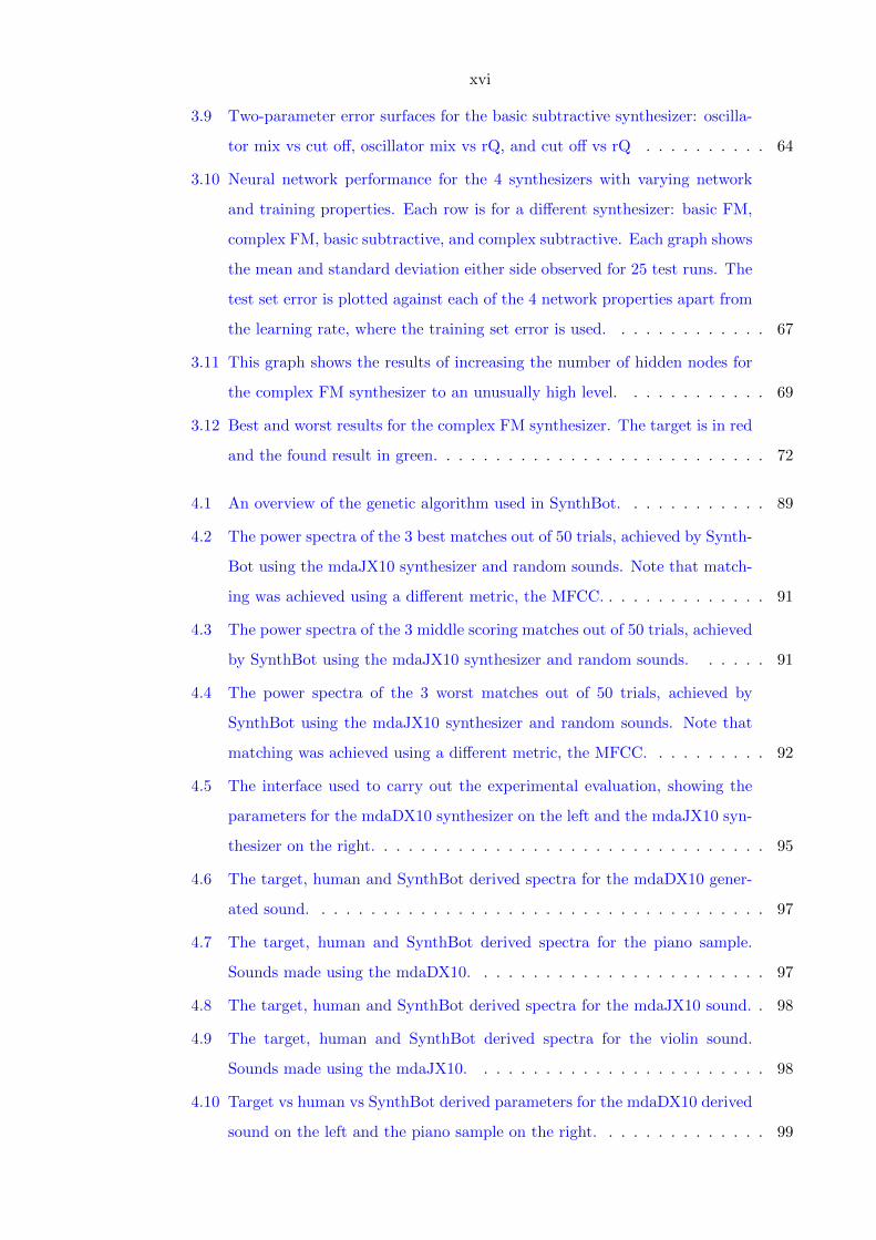
3.1 This image shows the distances in MFCC feature space between the ten

instrument samples used as targets for the optimisers. The higher the value,

the greater the distance and therefore the dissimilarity. The left matrix

compares the attack portions of the instruments, the right compares the

sustain periods, defined as the first 25 feature vectors and feature vectors

50-75, respectively. . . . . . . . . . . . . . . . . . . . . . . . . . . . . . . . . 55

3.2 The error surface measured from a reference setting of [0.5, 0.5] for the basic

two parameter FM synthesis algorithm. . . . . . . . . . . . . . . . . . . . . 56

3.3 Zoomed plot of the error surface in the region between 0.4 and 0.6 for

parameter two of the basic FM synthesizer. . . . . . . . . . . . . . . . . . . 57

3.4 The error surface for the basic FM synthesizer. The colour indicates the

distance in feature space from audio generated with that parameter setting

to a reference feature generated with parameter settings 0.5, 0.5, hence the

global minimum error at 0.5,0.5. . . . . . . . . . . . . . . . . . . . . . . . . 58

3.5 The error surface measured from a reference setting of 0.5 for the 22 param-

eter, complex FM synthesis algorithm. In the left column, a switched-type

parameter, modulation routing for oscillator 1; in the centre, a continuous

parameter, modulation index from oscillator 1 to 2; on the right, a quantised

parameter, coarse frequency ratio for oscillator 1. . . . . . . . . . . . . . . . 59

3.6 Two-parameter error surfaces for the complex FM synthesizer: modula-

tion routing vs frequency ratio, modulation routing vs modulation index,

modulation index vs modulation routing. . . . . . . . . . . . . . . . . . . . 60

3.7 The error surface measured from a reference setting of [0.5, 0.5, 0.5] for the

basic three parameter subtractive synthesis algorithm. . . . . . . . . . . . . 62

3.8 The mix levels of each oscillator in the basic subtractive synthesizer as the

oscillator mix parameter is varied. Each oscillator can take on one of 10

mix levels. . . . . . . . . . . . . . . . . . . . . . . . . . . . . . . . . . . . . . 62

xvi

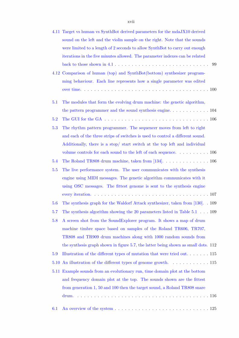
3.9 Two-parameter error surfaces for the basic subtractive synthesizer: oscilla-

tor mix vs cut off, oscillator mix vs rQ, and cut off vs rQ . . . . . . . . . . 64

3.10 Neural network performance for the 4 synthesizers with varying network

and training properties. Each row is for a different synthesizer: basic FM,

complex FM, basic subtractive, and complex subtractive. Each graph shows

the mean and standard deviation either side observed for 25 test runs. The

test set error is plotted against each of the 4 network properties apart from

the learning rate, where the training set error is used. . . . . . . . . . . . . 67

3.11 This graph shows the results of increasing the number of hidden nodes for

the complex FM synthesizer to an unusually high level. . . . . . . . . . . . 69

3.12 Best and worst results for the complex FM synthesizer. The target is in red

and the found result in green. . . . . . . . . . . . . . . . . . . . . . . . . . . 72

4.1 An overview of the genetic algorithm used in SynthBot. . . . . . . . . . . . 89

4.2 The power spectra of the 3 best matches out of 50 trials, achieved by Synth-

Bot using the mdaJX10 synthesizer and random sounds. Note that match-

ing was achieved using a different metric, the MFCC. . . . . . . . . . . . . . 91

4.3 The power spectra of the 3 middle scoring matches out of 50 trials, achieved

by SynthBot using the mdaJX10 synthesizer and random sounds. . . . . . 91

4.4 The power spectra of the 3 worst matches out of 50 trials, achieved by

SynthBot using the mdaJX10 synthesizer and random sounds. Note that

matching was achieved using a different metric, the MFCC. . . . . . . . . . 92

4.5 The interface used to carry out the experimental evaluation, showing the

parameters for the mdaDX10 synthesizer on the left and the mdaJX10 syn-

thesizer on the right. . . . . . . . . . . . . . . . . . . . . . . . . . . . . . . . 95

4.6 The target, human and SynthBot derived spectra for the mdaDX10 gener-

ated sound. . . . . . . . . . . . . . . . . . . . . . . . . . . . . . . . . . . . . 97

4.7 The target, human and SynthBot derived spectra for the piano sample.

Sounds made using the mdaDX10. . . . . . . . . . . . . . . . . . . . . . . . 97

4.8 The target, human and SynthBot derived spectra for the mdaJX10 sound. . 98

4.9 The target, human and SynthBot derived spectra for the violin sound.

Sounds made using the mdaJX10. . . . . . . . . . . . . . . . . . . . . . . . 98

4.10 Target vs human vs SynthBot derived parameters for the mdaDX10 derived

sound on the left and the piano sample on the right. . . . . . . . . . . . . . 99

xvii

4.11 Target vs human vs SynthBot derived parameters for the mdaJX10 derived

sound on the left and the violin sample on the right. Note that the sounds

were limited to a length of 2 seconds to allow SynthBot to carry out enough

iterations in the five minutes allowed. The parameter indexes can be related

back to those shown in 4.1 . . . . . . . . . . . . . . . . . . . . . . . . . . . . 99

4.12 Comparison of human (top) and SynthBot(bottom) synthesizer program-

ming behaviour. Each line represents how a single parameter was edited

over time. . . . . . . . . . . . . . . . . . . . . . . . . . . . . . . . . . . . . . 100

5.1 The modules that form the evolving drum machine: the genetic algorithm,

the pattern programmer and the sound synthesis engine. . . . . . . . . . . . 104

5.2 The GUI for the GA . . . . . . . . . . . . . . . . . . . . . . . . . . . . . . . 106

5.3 The rhythm pattern programmer. The sequencer moves from left to right

and each of the three strips of switches is used to control a different sound.

Additionally, there is a stop/ start switch at the top left and individual

volume controls for each sound to the left of each sequence. . . . . . . . . . 106

5.4 The Roland TR808 drum machine, taken from [134]. . . . . . . . . . . . . . 106

5.5 The live performance system. The user communicates with the synthesis

engine using MIDI messages. The genetic algorithm communicates with it

using OSC messages. The fittest genome is sent to the synthesis engine

every iteration. . . . . . . . . . . . . . . . . . . . . . . . . . . . . . . . . . . 107

5.6 The synthesis graph for the Waldorf Attack synthesizer, taken from [130]. . 109

5.7 The synthesis algorithm showing the 20 parameters listed in Table 5.1 . . . 109

5.8 A screen shot from the SoundExplorer program. It shows a map of drum

machine timbre space based on samples of the Roland TR606, TR707,

TR808 and TR909 drum machines along with 1000 random sounds from

the synthesis graph shown in figure 5.7, the latter being shown as small dots. 112

5.9 Illustration of the different types of mutation that were tried out. . . . . . . 115

5.10 An illustration of the different types of genome growth. . . . . . . . . . . . 115

5.11 Example sounds from an evolutionary run, time domain plot at the bottom

and frequency domain plot at the top. The sounds shown are the fittest

from generation 1, 50 and 100 then the target sound, a Roland TR808 snare

drum. . . . . . . . . . . . . . . . . . . . . . . . . . . . . . . . . . . . . . . . 116

6.1 An overview of the system . . . . . . . . . . . . . . . . . . . . . . . . . . . . 125

xviii

6.2 An instance of an additive synthesis algorithm. This algorithm utilises

three oscillators so would be encoded with 3 genes. Note that there is no

redundancy in this synth graph – every unit generator affects the resulting

audio signal. . . . . . . . . . . . . . . . . . . . . . . . . . . . . . . . . . . . . 126

6.3 An instance of an FM synthesis algorithm. This algorithm uses 4 oscil-

lator/ envelope blocks so would be encoded with 4 genes. Note that the

genetic encoding permits redundancy in the synth graph where not every

unit generator affects the resulting audio signal . . . . . . . . . . . . . . . . 126

6.4 An evolutionary run showing fitness against iteration for a moving target.

This is from an early version of the improviser which used a power spectrum

based fitness function. The points at which the target changes are associated

with large falls in fitness. . . . . . . . . . . . . . . . . . . . . . . . . . . . . 132

1

Chapter 1

Introduction

This thesis investigates techniques for the exploration and representation of digital sound

synthesis space, the space of possible sounds that a synthesis algorithm can produce.

Following that, it presents several interactive applications of these techniques. The thesis

is situated in the cross-disciplinary field of computer music; it uses search and optimisation

algorithms from computer science, descriptions of the human perceptual pathways from

psychology and neuroscience and the audio manipulations made possible by digital signal

processing. These streams are contextualised within the author’s practise as a composer,

programmer and performer.

In 1969, Mathews asserted that the main problems facing the computer musician were

the computing power needed to process the complex data representing a pressure wave

and the need for a language capable of succinctly describing this data for musical purposes

[76]. In 1991, Smith stated that the computing requirements had been met but that the

language problem persisted:

Problem 2 remains unsolved, and cannot, in principle, ever be completely

solved. Since it takes millions of samples to make a sound, nobody has the

time to type in every sample of sound for a musical piece. Therefore, sound

samples must be synthesized algorithmically, or derived from recordings of

natural phenomena. In any case, a large number of samples must be specified

or manipulated according a much smaller set of numbers. This implies a great

sacrifice of generality. (Smith 1991 [111])

Many computer music languages have been conceived, essentially for the purposes of

describing and controlling sound synthesis algorithms. They range from the lightweight

MIDI protocol with its note and control data, through graph based languages such as the

2

Max family, 1 to text based languages such as CSound 2 and SuperCollider [98, 126, 78].

These languages provide sophisticated ways to control sound within a lower dimensional

space than that of the individual samples constituting the digital signal, but what is

Smith’s generality which is lost? One interpretation is that as soon as you start using

a particular synthesis technique, you are limiting your sonic range to far less than the

total range available in a digital system. This is true even if the limitation is that you

are using what seems like a highly generalised abstraction of sound synthesis such as the

unit generator/ synth graph model found in SuperCollider and Music N languages. If

we consider the computer as an instrument, this loss of generality is not anything new;

traditional instruments do not provide complete sonic generality but by limiting the player

within their physical constraints, provide a challenge to the inventiveness of composer and

musician. Collins notes that traditional instruments offer highly evolved user interfaces

which enable a tight coupling between musician and instrument [24, p. 10]. Perhaps we

should accept the computer music language as the equivalent - a highly evolved interface

between human and machine as opposed to an immediately limiting means with which to

construct streams of samples. Either way, the challenge for a computer music language,

or a computer music utility, is to provide access to a much larger range of sounds than a

traditional instrument can produce, via some sort of interface. The interface might be a

graphical user interface or something more abstract such as the semantic elements of the

language combined with its sound synthesis libraries.

In a discussion of the future directions for computer music (languages) from 2002,

Scaletti introduces the ideas of ‘the space’ and ‘the path’ as the two parts of a new

artwork [105]:

The space of an artwork can be anything from a physical, three-dimensional

space (where the dimensions would be time-stamped x, y, and z coordinates) to

a completely abstract higher- dimensional space (where the dimensions might

be the allowed pitch classes or timbral characteristics).

...

A path through the space can be a predetermined or recorded path chosen by

the artist (as in an acousmatic tape piece, a film, or a theme-park ride where

the participants sit in cars pulled along tracks). Alternatively, it can be a live

path (or paths) where the audience and/or improvising performers explore the

1Named after Max Mathews.2The culmination of Mathews’ ‘Music N’ series of languages.

3

space interactively. (Scaletti 2002 [105])

In the case of music, the composer defines the space and the listener or improvising

musician defines the path through that space. McCartney denotes the motivations for

the design of the SuperCollider language as ‘the ability to realize sound processes that

were different every time they are played, to write pieces in a way that describes a range

of possibilities rather than a fixed entity, and to facilitate live improvisation by a com-

poser/performer.’ [78]. This appears to fit in rather well with Scaletti’s definition of the

modern art form of computer music and SuperCollider provides an impressive range of

unit generators and language constructs to support this activity.

So computer music languages provide many ways to design synthesis algorithms (the

space) and many ways to control and explore them (the path) but they do not really shed

any light on the complete range of sounds that a particular algorithm can make. Could

this be another aspect of the limited generality Smith is talking about, that a musician

is not even able to fully exploit a synthesis algorithm, once they have limited themselves

within its constraints? For example, using SuperCollider it is trivial to implement an FM

synthesizer with an arbitrary number of operators and to feed in parameter settings in a

complex, algorithmic way. The synthesizer is certainly capable of generating a wide range

of sounds, but the language does not provide a means by which to make a particular sound

with that synthesizer or any information about its full sonic range.

Aside from specialised languages, the other method of working with computer music

is the utility, a program that typically models some well known music production process,

e.g. Cubase modelling a multi-track recording set up [105]. The use of the computer in

contemporary music production processes is near ubiquitous and likewise these utilities.

Whilst it is not always their main focus, they also attempt to make the range of possible

sounds from a digital system more accessible, especially through the use of plug-in effects

and synthesizers. Again, the limitations of their interfaces and sound design paradigms

might be limiting the composer’s sonic potential.

Could a natural extension to these languages and utilities be an analysis system capable

of taking a synthesizer and splaying it out upon the composer’s workbench, such that its

full sonic range is made accessible? In this way, can one claim to have regained some

generality in sound synthesis? The work in this thesis aims to suggest the form of such a

synthesizer analysis system, a system which can assess, present and search the full sonic

range of an arbitrary synthesis algorithm. The impact of this system on the practise of

computer musicians is then assessed by constructing and trialling new tools based upon

4

it.

1.1 Research Context and Personal Motivation

This section provides a brief review of the supporting literature for the main research

themes in the thesis followed by an exposition of the author’s personal motivation for

carrying out this work.

Describing Timbre

In order to assess, present and search the space of possible sounds for a synthesizer, it is first

necessary to consider the nature of timbre and how this might be represented numerically.

Chapter 2 presents the accepted view of the human ascending auditory pathway, derived

mainly from Moore’s seminal text and the excellent collection of articles edited by Deutsch

[88, 32]. Definitions of timbre are taken from Risset and Wessel, Thompson and Pitt and

Crowder; essentially, they agree, timbre is everything left after normalisation for loudness

and pitch [32, 123, 97]. A selection of classic and recent studies which attempt to measure

timbral distance using listener based experiments are discussed in this chapter, including

the work of Crowder and Halpern et al. [29, 43]. People do tend to concur regarding

the level of similarity between instruments but timbre is not easily separated from other

factors such as pitch. Many studies have attempted to ascertain the salient aspects of a

signal with regard to the human ability to differentiate timbres [6, 63, 57]. The conclusion

seems to be that given an appropriate experiment, it can be shown that most aspects of

a note played on a musical instrument can be shown to contribute to a listener’s ability

to identify the source instrument.

The detailed description of the Mel Frequency Cepstrum Coefficient (MFCC) feature

vector in chapter 2.4 is derived from Davis and Mermelstein [31]. The MFCC, whilst orig-

inally designed for speech recognition tasks, is a widely used feature for timbre description

and instrument recognition, e.g. see Casey et al. and Eronen [16, 33]. Combining the

MFCC with a listener test, Terasawa et al. were able to reinforce the validity of the MFCC

as a measure of timbre, as they were able to correlate distances in MFCC space with per-

ceived distances between sounds [121]. The comparison of open source implementations of

MFCC feature extractors in subsection 2.4.3 uses code from Collins, Bown el al., Schedl

and Bullock [25, 12, 106, 15].

5

Mapping and Exploring Timbre Space

Having established the basis for numerical descriptions of timbre, the concept of mapping

and exploring timbre space is introduced. This concept can be traced through the research

literature as well as appearing in commercial synthesizer implementations. Several of the

timbre measurement studies mentioned earlier present the results of human-derived timbre

similarity data using a dimensionally reduced map. Examples of these maps, taken from

Gray, Iverson et al. and Halpern et al., are provided in figure 2.1 [42, 57, 43]. For reference,

a compact guide to the technique of multidimensional scaling, along with other methods

for dimensional reduction is provided by Fodor [35].

Applying the concept of dimensional reduction to synthesizer control, Bencina’s Meta-

surface system provides a means for locating and interpolating between sounds of interest

[7]. Metasurface provides a two dimensional space for exploration by the user that is

mapped to a higher dimensional parameter space by means of a parametric interpolation

technique. Stowell’s work mapping vocal features to sound synthesizer parameters with

self organising maps is a more recent example of this dimensional reduction applied to

synthesizer control [117].

Aside from the almost ubiquitous ‘knobs and sliders’ user interfaces, commercial sys-

tems do not seem to offer many alternative approaches to exploring synthesizer timbre

space, beyond large, hierarchically categorised banks of presets like those found in Native

Instruments’ ‘KoreSound Browser’ and Aturia’s ‘Analog Factory’ [56, 4]. Possibly the

most progressive commercially available tool is Dahlstedt’s ‘Patch Mutator’ found in the

Nord Modular G2 programmer, which uses an interactive genetic algorithm to empower

the user to explore sound synthesis space more dynamically [30]. Similar applications of

interactive GAs to sound synthesizer design have been seen many times in the literature,

for example see Johnson’s CSound based system, Collins’ SuperCollider based system or

the author’s Java based AudioServe [59, 23, 136].

Automatic Synthesizer Programming

Another aspect of having a generalised description of sound synthesis space is the ability

to search for a specific sound in that space. Automated synthesizer programming aims to

find the parameter settings for a synthesizer which cause it to produce as close as possible

a sound to a given target. Interestingly, a patent for an iterated process of sound synthe-

sizer parameter optimisation was filed in 1999 by Abrams [1]. Prior art can be found is

Horner et al’s seminal journal article on the topic from 1993 where the researchers achieve

6

automated tone matching using a genetic algorithm and FM synthesis [48]. Subsequent

reports of genetic algorithms being applied to automated sound synthesizer programming

problems are multitudinous. Garcia (2001) used a tree based genetic programming model

to evolve variable synthesis graphs [39]. Mitchell el al. (2005) extended Horner’s work with

fixed architecture FM synthesis using more sophisticated evolutionary algorithms [87]. Lai

et al. (2005) revisited Horner’s FM tone matching, deploying the spectral centroid fea-

ture in place of the power spectrum [67]. Johnson and Gounaropoulos’ system (2006)

evolved sounds to a specification in the form of weighted timbre adjectives [40]. Chinen’s

Genesynth (2007) evolved noise and partial synthesis models, and is one of the few systems

available in source code form [18]. McDermott (2008) focused on the use of interactive

GAs to enhance human synthesizer programing capabilities but also addresses the fixed

synthesis architecture, automatic tone matching problem [80]. Miranda provides a paper

summarising advancements circa 2004 and along with Biles provide an excellent selection

of papers up to 2007 about the application of evolutionary computation to music in gen-

eral [85, 86]. It seems that the literature on automated sound synthesizer programming

is dominated by evolutionary computation, especially with regard to parametric optimi-

sation for fixed architecture synthesizers, but there are other methods of resynthesis. The

classic analysis/ resynthesis combination is Serra and Smith’s spectral modeling synthe-

sis, which reconstructs a signal using partials and noise [109]. Schwarz’s concatenative

corpus-based resynthesis constructs a simulacrum of a signal using fragments taken from

a pre-existing corpus of recorded material, where the fragments are chosen using a feature

vector similarity metric [108]. Sturm et al. reduce this recorded corpus to a collection of

simple functions, then provide a means to deconstruct a signal into an even finer patch-

work made from the outputs of these functions [118]. In other words, they provided the

missing analysis stage for granular synthesis, making it possible to granularly resynthesize

pre-existing signals.

Interactive Music Systems

In chapters 4, 5 and 6, applications of tone matching techniques are described. These

applications employ autonomous processes in varying degrees as part of the compositional

process. Therefore the systems are examples of interactive music systems. Rowe provides

a classification system for interactive music systems, wherein he describes points along

three different continua [104]:

1. score-driven/performance-driven. How is the system driven? Does it work from a

7

score or does it respond to/ generate a performance?

2. transformative/generative/sequenced. How does the system derive its output? Does

it transform pre-existing material, generate new material or read from a sequence?

3. instrument/player paradigms. Is the system an extension to an instrument or a

player in its own right?

SynthBot, the automatic synthesizer programmer described in chapter 4 is an extension

to the synthesizer instrument, a tool with which to better program the synthesizer. The

evolving drum machine described in chapter 5 is also an extension to the synthesizer

instrument but it adds the extra dimension of transformation, since the emphasis is on

the change in timbre over time. The timbre matching improviser described in chapter 6

falls at a different end of the instrument/ player continuum to the other systems: it is

an autonomous player. It is performance driven as there is no pre-existing score other

than that provided during the performance by human musician and it can be described

as transformative, since it works with material provided by the human player during the

performance. Hsu describes a related system which improvises by generating a series

of timbral gestures that are similar to those generated by the human performer [50].

One difference is that Hsu’s system is entirely timbre based. which is in keeping with

the playing style of saxophonist John Butcher with whom it was developed. Another

difference is that it is semi-autonomous: ‘In our initial design discussions, John Butcher

emphasized that there should be options for a human to influence at a higher level the

behavior of the virtual ensemble’, states Hsu. An updated system known as the ARHS

system reduced the need for human input using a more elaborate performance controller

with hierarchically organised performance statistics [51]. Of this new system, Hsu notes:

‘...it coordinates more effectively high and low level performance information, and seems

capable of some musically interesting behavior with little human intervention’. Collins

describes a completely autonomous multi-agent ‘Free Improvisation Simulation’, which

uses onset and pitch detection as its listening components and comb filter based physical

modelling to synthesize its guitar-like output. [24, p. 178-184]. Ian Cross, the guitarist who

played with it, described the experience as like being ‘followed by a cloud of mosquitoes’,

which provides an insight into its sound output. Cross’s main issue was that ‘whereas the

system could react to the microstructure of his performance effectively, it did not pick

up larger-scale structures’, precisely the problem Butcher wished to sidestep by enabling

high level human intervention. The ability to detect meaningful information about larger

scale structures is a major challenge to such systems, one which is addressed in Collins’

8

later work through the use of on line machine learning during an improvisation [21]. For

further expositions about interactive music systems, the reader is referred to Rowe’s book

and Collins’ PhD thesis, where a further discussion of this topic and related research can

be found [104, 24].

Personal Motivation

In his activities as a practitioner of electronic music, the author has found certain regions

of the terrain to be of interest in an artistic and technical sense simultaneously, where the

demands placed on his creativity are equal in both. These regions are typically located at

the challenging points of crossover between technical and artistic activity, where the desired

output cannot be achieved without some sort of creative technical endeavour. Synthesizing

sounds is a key part of the electronic musician’s technique. About a third of Roads’ 1000

page masterpiece, ‘The Computer Music Tutorial’ is dedicated to it [102]. In his definition

of his own creative practise, ‘Manifesto of Mistakes’, the contemporary composer and DJ

Matthew Herbert emphasises the importance of using sounds that did not exist previously,

specifying the avoidance of preset sounds and patches [45]. So sound synthesis is a core

part of computer music and its practitioners show an interest in unheard before sounds.

Further, sound synthesis sits exactly at one of these crossover points between art and

technique, presenting the practitioner with the following questions: ‘Is this sound good?’

and ‘How can I make it better?’. Exploring sound synthesis space rapidly and exhaustively

is not currently possible within commercial synthesizer programming interfaces but success

has been reported using esoteric research systems, as mentioned in the previous sections. If

this timbral exploration can be made possible, with new frameworks and industry standard

tools, a new vista of timbres can be placed within the grasp of musicians who can then

conduct a virtuosic exploration of electronic sound.

1.2 Research Questions

In this section, the perceived problems which are investigated in this thesis are stated and

described in the form of several questions. In the conclusion section 7.1, these problems

are re-iterated and the success of the thesis in answering them is assessed.

Problem 1: Numerical Representations of Timbre

What is meant by the term timbre? What is the ideal way to represent timbre? There

is an extensive body of research which attempts to define the nature of the perception

9

of timbre; it seems that the limitations of the human hearing apparatus and timbre’s

inseparability from pitch make it difficult to isolate. If we accept that it can be isolated

to some extent, how can it then be measured and represented numerically? What is the

best feature vector to use that is capable of differentiating between timbres? Further,

does the feature vector offer a smooth transition through feature space, where movement

in numerical feature space equates to a similarly weighted movement in perceptual space?

Problem 2: Effective Sound Synthesizer Programming

Old fashioned analog synthesizers had interfaces which encouraged an exploratory method

of programming with their banks of knobs and sliders. What is involved in this explo-

ration? Is this an effective method to use when a specific sound is required? Is the user

making full use of the capabilities of their synthesizer, i.e. is the piano sound they have

made the best piano sound the synthesizer can make? Some recent synthesizers can have

over 1000 parameters - what is an appropriate interface to use here and is the user likely

to be able to fully exploit the synthesizer using it?

Problem 3: Mapping and Describing Sound Synthesis Space

What happens to the timbre of a synthesizer as the parameter settings are varied? Does

the timbre change smoothly from place to place in the synthesizer’s timbre space? What

is an appropriate resolution to use when examining timbre space? Is there some way to

create a map of the complete timbre space of a synthesizer? Can this be used to improve

the user’s ability to exploit it?

Problem 4: Searching Sound Synthesis Space or Automated Synthesizer

Programming

Automated synthesizer programming involves automatically finding the best parameter

settings for a given sound synthesizer which cause it to produce as close a sound as

possible to a specified target sound. What is the best algorithm to use to search sound

synthesis space and find the optimal settings? What additional challenges are posed by the

requirement to automatically program existing synthesizers? E.g. can a general method

be developed for the automated programming of a large body of existing synthesizers?

10

Problem 5: Creative Applications of the Above

The final problem is how to apply techniques and systems developed in response to the

previous problems in a creative context and then how to evaluate them. The creative

context might be a standard synthesizer programming task, where the system must fit

into the usual work flow of the user, by integrating with industry standard tools. Or the

aim might be to innovate a new creative context where the systems and techniques are

used to compose or improvise in new ways. In each of these contexts, what demands are

placed on the underlying technology and how should it be adapted to meet these demands?

1.3 Aims and Contributions

The original work presented in this thesis contributes a variety of systems and analyses

to the research fields mentioned in section 1.1. The conclusion section 7.2 revisits the

following list and refers to the specific areas of the thesis wherein these contributions are

made. The contributions are as follows, in no particular order:

1. An assertion of the validity of the Mel Frequency cepstrum Coefficient as a timbral

descriptor.

2. A comparison of open source MFCC extractors.

3. New methods for describing, visualising and exploring timbre spaces.

4. A comparison of methods for automatically searching sound synthesis space.

5. A synthesis algorithm-agnostic framework for automated sound synthesizer program-

ming compatible with standard studio tools.

6. A comparison of human and machine synthesizer programming.

7. A re-invigorated drum machine.

8. A timbre matching, automated improviser.

Beyond the questions posed in section 1.2, the thesis can be framed in terms of a set of

aims. In the achieving of these aims, the thesis will be able to answer those questions and

provide a set of new tools to computer musicians. The aims are detailed in the following

subsections, along with pointers to the relevant parts of the thesis:

11

Establish the Best Method for Numerical Representation of Timbre

To this end, an overview of the ascending auditory pathway is provided in chapter 1,

followed by a discussion of a wide range of previous work investigating the perception and

imagination of timbre. An ideal numerical measure of timbre is characterised and the Mel

Frequency Cepstrum Coefficient is presented as a widely used, general purpose feature for

representing timbre which matches well to the ideal representation. Open source MFCC

feature vector extractors are compared and a new, reference implementation is described.

Explore Ways of Representing and Describing Timbre Space

In section 2.5 a new tool is introduced which allows the user to view large parts of the

complete timbre space for a given synthesizer or set of samples. The tool, SoundExplorer,

uses the Multidimensional Scaling technique to place high dimensional feature vectors into

a 2 dimensional space such the user can view and rapidly explore the space. In chapter 3,

the concept of a timbral error surface is introduced, which makes it possible to describe

the effects of parametric variations on the timbre of a synthesizer.

Analyse Techniques for Search of Timbre Space

Chapter 3 presents 4 techniques that can be used to search timbre space. The techniques

are compared in their ability to find sonic targets that are known to be in the space and to

find best approximations for real instrument targets which are not likely to exist precisely

in the space.

Compare Synthesis Algorithms for Tone Matching Purposes

Chapter 3 compares fixed architecture FM synthesis, subtractive synthesis and variable

architecture FM synthesis algorithms in their ability to match real instrument timbres.

Deploy Tone Matching Techniques Using Industry Standard Tools

Chapter 4 presents SynthBot, which is a tone matching program that can search for

parameter settings for any sound synthesizer available in the VST plug-in format. The

system is evaluated for its performance with two different plug-ins.

12

Compare Human and Machine Synthesizer Programming Behaviour and

Ability

Chapter 4 presents the results of a user trial where human synthesizer programmers were

compared to SynthBot in their ability to search for sounds known to be in the space as

well as real instrument sounds.

Re-invigorate Venerable Studio Tools - the Drum Machine and the Syn-

thesizer

Chapter 5 discusses the implementation of an evolving drum machine, where the sounds

evolve from random start points toward user specified target sounds whilst the user is

programming rhythms for the machine. The results of an evaluation with two experienced

drum machine users are also given. The synthesizer is re-invigorated at various points in

the thesis, in two principal ways: automated synthesizer programming and through the

creation of timbral maps. The former method is explored in chapters 3,4 5 and 6, the

latter mainly in chapter 2.

Investigate Creative Effects of Search Algorithm Variations

Chapter 5, subsection 5.6.2 discusses the creative effects of different aspects of the genetic

algorithm used to evolve sounds in the drum machine, such as mutation types, genomic

growth operations, population sizes and so on. Chapter 6 subsection 6.3.1 explores some

of these ideas further, with a different application of the timbre space exploration.

Create an Automated Melodic and Timbral Improviser

Chapter 6 details the implementation of an automated improviser which uses a genetic

algorithm driven sound synthesis engine. The system is evaluated in terms of its success

as a useful musical tool and its appearance in various radio and recording sessions. Some

reflection on the use of the system is provided from the author and a musician who has

played several times alongside the automated improviser.

1.4 Methodology

In this section, the methodology employed to carry out the reported work is explained.

The methodology falls into 3 categories: software development, numerical evaluation and

user trials.

13

1.4.1 Software

The software used to carry out the research under discussion here has been programmed in

a variety of software environments. Details of the implementation of the various systems

are provided as required in the thesis. In summary, the following technologies have been

used:

1. The Java language. Java was the main language used for software development. Syn-

thBot (chapter 4), SoundExplorer (chapter 2), the Evolving Drum Machine (chapter

5) and the Automated Improviser (chapter 6) used Java to some extent. Java was

also used extensively for batch processing and data analysis tasks.

2. The Java Native Interface (JNI) [72]. JNI was used to enable Java code to interact

with natively compiled plug-ins for the SynthBot system (chapter 4).

3. SuperCollider3 (SC3) [78]. SC3 was used as a sound synthesis engine for the Evolving

Drum Machine and the Automated Improviser (chapters 5, 6). The comparison of

sound synthesis space search techniques reported in chapter 3 was conducted using

a framework developed entirely in SC3.

4. Open Sound Control (OSC) [137]. OSC was used as a communication protocol to

connect the Java and SC3 parts of the software for the Evolving Drum Machine and

the Automated Improviser.

5. Virtual Studio Technology (VST) [115]. VST was used as the synthesizer plug-in

architecture for SynthBot in chapter 4. This made is possible to integrate SynthBot

with a huge range of pre-existing synthesizers.

6. The R language [52]. R was used to carry out multidimensional scaling and to

compute various statistics.

7. GNUplot plotting software [135]. GNUplot was used to create many of the graphs

used in the thesis.

8. The EMACS text editor [114]. This document was authored using Emacs and the

majority of the software used to carry out the research was developed using Emacs.

9. LATEX[68]. LATEXwas used to typeset this thesis.

10. The GNU/ Linux operating system [113]. The majority of this work was carried

out using this open source operating system, aside from cross platform testing for

SynthBot.

14

Testing techniques have been used to verify the behaviour of the software, for example

passing a variety of test tones through MFCC extractors and verification of unexpected

results.

1.4.2 Numerical Evaluation

Many of the research findings and analyses were derived through numerical evaluations of

systems. Where stochastic algorithms have been used, results have been verified through

repeated runs and this is reported in the text. A variety of methods have been used to

represent the sometimes extensive data sets such as standard plots, heat plots, histograms

and so on.

1.4.3 User Trials

User trials were carried out in formal and informal ways. In chapter 4 SynthBot was

evaluated by comparing its performance to that of human synthesizer programmers. In this

case, the author visited each of the subjects in turn and carried out the trial. The user trials

of the Evolving Drum Machine reported in chapter 5 were carried out after the Conceptual

Inquiry model which takes a somewhat anthropological approach by conducting trials of

the system in its target context and reporting the observations made by the subject as

they interact with the system, lightly prompted by the researcher [47]. User trials of the

Automated Improviser described in chapter 6 were quite informal and very contextual,

enabling a reflective view of the system and its use in real world scenarios such as live

performance.

1.5 Thesis Structure

The thesis is organised into seven chapters. Chapter 2 is entitled ‘Perception and Rep-

resentation of Timbre’ and it aims to explain how timbre is perceived, to establish the

meaning of timbre and to suggest how timbre might be represented numerically. It also

contains a comparison of MFCC feature extractors and it concludes by presenting a new

tool which uses MFCCs and a dimensional reduction to present complete maps of sound

synthesizer timbre spaces. Chapter 3 is entitled ‘Searching Sound Synthesis Space’ and

its aim is to present the results of a detailed examination of sound synthesis space and

a comparison of automated sound synthesizer programming techniques. Chapter 4 is en-

titled ‘Sound Synthesis Space Exploration as a Studio Tool: SynthBot’. It describes the

15

first application of automated sound synthesizer programming along with a user trial pit-

ting expert human synthesizer programmers against the automated system. Chapter 5

is entitled ‘Sound Synthesis Space Exploration in Live Performance: The Evolving Drum

Machine’. It presents the second application of sound synthesis space search along with the

results of user trials of the system. Chapter 6 is entitled ‘The Timbre Matching Improviser’

and it describes the final application of automated sound synthesizer programming which

is an autonomous musical agent. Feedback from a musician who has played frequently

alongside the system is provided, along with some reports of its use in recording and radio

sessions. Finally, chapter 7 assesses the success of the thesis in answering the questions

posed in the present chapter, highlights where the major contributions have been made

and discusses possibilities for future work.

16

Chapter 2

Perception and Representation of

Timbre

This chapter provides an overview of the ascending auditory pathway, combining informa-

tion from standard texts with some more recent studies. The meaning and perception of

timbre is discussed and classic and recent experiments investigating the question of tim-

bral similarity are described. The properties of an ideal numerical measure of timbre are

suggested; the MFCC feature is described in detail and each part of the extraction pro-

cess is justified in terms of data reduction and perceptual relevance. Several open source

implementations of MFCC extractors are compared and a new Java implementation is

presented. Finally, inspired by the methods used to analyse and present results in sev-

eral previous timbre similarity experiments, a new tool for the exploration of the timbral

space of synthesizers and sample libraries based on dimensional reduction techniques is

described.

2.1 The Ascending Auditory Pathway

In this section, an overview of the mammalian ascending auditory pathway is provided, in

order to establish the grounds for the later discussion of numerical and other descriptions

of timbre.

In the mammalian auditory system, the ‘ascending auditory pathway’ is the term used

for the path from the ear, which physically senses sound waves, through to the auditory

cortex, where responses to complex stimuli such as noise bursts and clicks are observed

[88, p. 49]. In summary, the pathway leads from the three parts of the ear, (outer, middle

and inner) onto the basilar membrane (BM) of the cochlea via the auditory nerve to sites

17

in the brain stem (cochlear nucleus, trapezoid body, superior olivary nucleus, nuclei of the

lateral lemniscus), then sites in the mid brain (inferior colliculus and medial geniculate

body) and finally on to the auditory cortex (primary and secondary fields)[32, p. 48-53].

This is considered the ‘classic view of auditory information flow’ [70]. More recent work

has shown the true picture to be more complex, involving parallel pathways heading back

and forth; but the nature of this complex descending pathway is not as yet fully described.

In the following discussion, the established and well described ascending pathway will be

considered. All parts of this pathway might be considered relevant to the discussion of a

numerical representation of timbre and here follows a discussion of these parts.

2.1.1 From Outer Ear to Basilar Membrane

Sound waves hitting the outer ear eventually travel to the inner ear (cochlea) where they

vibrate the BM. Waves of different frequencies cause varying size vibrations at different

positions of the membrane, where the frequency to position mapping is logarithmic. Pi-

oneering work with human cadavers by von Bekesy, wherein the cadavers were blasted

with 140dB sine tones and had the vibrations of their BMs stroboscopically illuminated

and measured 1, provided the first description of the frequency response of the BM [127].

The response of the BM of a cadaver is somewhat different to that of the living so more

recent experiments with living specimens have been necessary. This work has elicited very

accurate measurements for the sites of frequency response of the BM. In terms of the

limitations of this apparatus, the BM vibrates at different points in response to different

frequency sound waves and as those different frequencies become closer to each other, so

do the positions of the vibrations. At a certain point, the separate frequencies are no

longer resolved and a single, large displacement of the BM is observed. Two frequencies

that are not resolved are said to lie within a critical band.

2.1.2 From Basilar Membrane to Auditory Nerve

The transduction of vibrations of the BM into neuronal activations is carried out by

the stereocilia of the inner hair cells. Movement of the BM causes movement of the

stereocilia of the inner hair cells which in turn causes them to release neurotransmitters

to the connected neurons. The outer hair cells are thought to provide fine, active control

of the response of the BM and are linked into higher level brain function [88, p. 32-

1To those who have attended a modern electronic music festival, this may seem to be a reasonably

’real-world’ scenario both in terms of the specimens and stimuli.

18

34]. Since vibrations in different parts of the BM affect different groups of inner hair

cells and the position of these vibrations depends on frequency, the neurons effectively

have different frequency responses. More properly, neurons in the auditory pathway are

said to have a receptive field which is defined in terms of their frequency and amplitude

response and which differs from neuron to neuron. The characteristic frequency (CF)

of a neuron is that which excites it at threshold amplitude, the best frequency (BF)

for a given amplitude is that which produces the greatest response. Throughout the

ascending auditory pathway, from the auditory nerve to the auditory cortex, neurons are

arranged tonotopically where neighbouring neurons have similar CFs. The arrangement

is logarithmic in terms of frequency [93], which is the same as the mapping of frequency

response of the BM in the cochlea. A further characteristic to note is that the bandwidth

of the frequency response increases with amplitude [73].

2.1.3 From Auditory Nerve to Auditory Cortex: Information Represen-

tation

At the next level of organisation, it becomes pertinent to begin talking in terms of in-

formation flow. Some researchers consider the auditory pathway as a series of informa-

tion processing stations wherein the auditory stimulus is transformed into different forms.

Chechik et al. investigate the ‘representation’ of the auditory stimulus at various points

along the auditory pathway of an anaesthetised cat by monitoring the responses of single

neurons [17]. The neurons were measured in the later stages of the pathway: the infe-

rior colliculus (IC), the auditory thalamus (medial geniculate body above/ MGB) and

the primary auditory cortex (A1) using mirco-electrodes. The stimuli were recordings of

birdsong issued in natural and modified states. The researchers found that information

redundancy reduced as the stimulus ascended the auditory pathway. An interesting ad-

ditional observation was the fact that neurons in the A1 showed responses to groups of

stimuli where the grouping criteria were not obvious from their tonotopic arrangement.

In earlier stages, as previously noted, there is a spectro-spatial grouping to the response,

where proximal neurons respond to proximal parts of the spectrum. Neurons in the A1

are seemingly more independent, responding to sets of stimuli with quite varied spectra,

suggestive of a higher level connection between stimuli. The criteria for the grouping of

sounds observed in the auditory cortex is unknown.

19

2.1.4 Sparse Coding of Auditory Information

A fairly recent development in neuroscience is the proposition of specific models that de-

scribe sparse coding schemes for the brain’s response to sensory stimuli. Sparse coding is

a phenomenon observed in neurological systems where a neural activation occurs within a

relatively small set of neurons or over a relatively short period of time [92]. The sugges-

tion is that it can be thought of as a highly optimised type of neural response or ‘neural

code’, one which can be said to ‘maximise the information conveyed to the brain while

minimizing the required energy and neural resources’ [110]. One study showed for the

first time that the response to sound of the unanesthetised rat auditory cortex actually is

sparsely coded [49]. The stimulus sounds were pure tones, frequency modulated sweeps,

white noise bursts and natural stimuli. The responses to the stimuli consisted of sparse

(defined as a response in < 5% of the neuron population at a time) bursts of high firing

rates in small groups of neurons. The researchers argue that the auditory cortex represents

sounds in the form of these sparse bursts of neuronal spiking activity. In ground breaking

work, a system that closely matched key properties of the auditory system, i.e. neuronal

frequency bandwidth and cochlear filter response, was derived, by optimising a nonlinear,

spike based model to represent natural sounds and speech [110]. In real terms, the re-

searchers were able to efficiently re-synthesize the word ‘canteen’ using 60 parameterised

spikes, generated from kernel functions. Compare this to a classical spectral representa-

tion which would encode ‘canteen’ using thousands of values. This model could provide

a very effective way to represent natural sounds numerically. Sparse coding has begun to

appear in the computer music literature, having, most famously, been used as a modelling

stage in granular synthesis [118]. An initial study using sparse coding as part of an instru-

ment recognition system directly compared performance between sparse coding and Mel

Frequency Cepstrum Coefficient (MFCC) based schemes. The MFCC worked well but not

as well as the sparse coding scheme [107]. However, the use of such schemes is beyond the

scope of the work presented here due to lack of any really commonly accepted or easily

used implementations.

As representations of timbre move beyond Fourier analysis in both the fields of neu-

roscience and computer music, will this be the end of the ‘classical view’ that timbre can

be described entirely in terms derived from the spectrum? [32, p. 114]

20

2.2 Defining Timbre and Timbre Perception

What is timbre? How can timbre perception and similarity be measured? In this section,

these questions will be addressed. Various definitions of timbre are provided; difficulties in

experimentally distilling the essence of timbre are discussed; the concept of imagined tim-

bre is introduced; finally, listener based timbre similarity experiments and their methods

of presenting results are described.

2.2.1 What is Timbre?

In terms of musical instruments, timbre is widely considered to be the remaining variation

that allows differentiation between instruments when pitch and intensity are constant.

That is, it is defined in terms of what it is not, not what it is:

Timbre refers to the quality of sound. It is the perceptual attribute that enables

us to distinguish among orchestral instruments that are playing the same pitch

and are equally loud. Risset and Wessel, [32, p. 113],

Timbre is often described as the attribute of distinguishing sounds that are

equivalent in pitch, duration and loudness. Thompson, [123, p. 59],

Timbre can be defined as the characteristic quality of a sound–other than its

pitch, loudness or duration–that identifies it uniquely (as a flute,violin,piano,etc.).

Pitt and Crowder, [97, p. 728],

If a tree falls in a forest but there is no-one there to hear it, what is its timber?

(Anon.).

2.2.2 Inseparability of Pitch and Timbre

Timbre and pitch are somewhat slippery though. Typically, pitch is considered to be the

fundamental frequency of a harmonic or near harmonic series. Perhaps this frequency

component is the one used by listeners to perceive pitch; but listeners can still judge pitch

in the absence of the fundamental frequency, f0 when it is missing [146]. Pitch should

be separate from timbre which, based on the definitions above, must be something that is

concerned with other aspects of the sound and their dynamics. Still, experiments where

listeners had to judge whether two notes or two chords were the same were affected by

the timbre [29], [5]. The listeners were typically played two sounds consecutively, asked

to state if they heard the same note or chord each time and the speed and accuracy of

their response was measured. If there was a timbral variation between the two sounds,

21

listeners found it harder to judge the similarity rapidly. In the chord experiment, non-

musicians’ performance degraded more than that of musicians when the timbre varied [5].

This suggested non-musicians were relying more on aspects beyond the fundamental to

identify pitch than were musicians or that in a pitch focused experiment, musicians were

able to focus more effectively on pitch. For the purposes of the work presented in this

thesis, the pitch can typically be made constant between differing timbres. For example,

consider the canonical problem here: ‘given a recording of an instrument and a synthesizer,

how must one program the synthesizer to make that instrument sound?’. It is possible to

detect the pitch of the target instrument recording and to use that pitch to choose the

note that the synthesizer is playing. The interference between timbre and pitch is worth

noting however, as this should be considered in the choice of a numerical representation

of timbre.

2.2.3 Imagining Timbre

Several of the experiments which analyse the effect of timbral variations on the perception

of pitch mention the idea of musical imagery, the act of a listener imagining a particular

note, melody, timbre etc.. In the second part of the two note, pitch testing experiment

mentioned above, listeners were played a sine tone followed by a real instrument tone and

asked to imagine how a particular instrument would have sounded in the gap between the

two stimulus sounds [29]. If the requested, imagined timbre was the same as the second

timbre, they responded more rapidly - imagining the timbre made it easier to track the

pitch. This was interpreted as timbre having an ‘interference effect’ on the perception

of pitch. As mentioned earlier, people can fill in the missing fundamental in order to

correctly identify pitch, so spectral content must be part of pitch perception, not just the

fundamental. The interference between timbre and pitch perception should not be too

surprising, then. In this experiment, it was not clear what the subjects were imagining:

were they imagining the way the instrument looked, sounded or something else? Since the

imagined instruments were different, it was difficult to make assertions here. Further work

by Pitt and Crowder showed that the interference effect of timbre upon pitch perception

was only present when the spectral aspects of the timbre were varied, not the dynamics

[97]. Noting that in the experiment, spectral properties were considered as constants in a

timbre, the researchers conclude thus:

We found that the image of a timbre appears to be based primarily on spectral

properties. No evidence was found that suggested that dynamic properties, at

22

least attack rate, are represented in an auditory image. [97, p. 737].

Is Imagining Timbre Sensory or Motor Based?

Pitt and Crowder state that their earlier work, where it was demonstrated that humans

can imagine timbres, was partly motivated by a desire to show that imagined timbre was

a sensory processing rather than a motor processing neural phenomenon [97], [29]. The

former can be thought of as ‘the mind’s ear’, where the sound is fully imagined whereas in

the latter the phenomenon is linked to a real or imagined motor process such as humming a

note. Since the human vocal tract cannot accurately reproduce most instrument timbres,

they argue, the ability to imagine the timbres of these instruments must be sensory, not

motor processing based 2. They showed that imagining timbre has a positive effect upon

pitch similarity judgement performance and therefore concluded that timbral imagery

must exist and that it must be sensory processing based.

More recent work investigating the nature of timbral imagery was carried out by

Halpern et al. [43]. In this extremely thorough study, they essentially analysed brain

activity when the subjects were making similarity judgements about real and imagined

timbres, using high resolution fMRI. They showed that the sites of activity when imagin-

ing single note timbres were similar to those activated by the perception of actual sounds.

Also, some activation sites were related to those for subvocal rehearsal (silent mental rep-

etition of stored vocal information), in other words, motor pathways. Whilst the latter

observation suggests the importance of motor pathway activations in timbral imagery, the

researchers leave the conclusion of the sensory/ motor question for further studies. This

work will be discussed in more detail along with related studies in the following subsection.

2.2.4 Listener-Based Timbre Similarity Experiments

There have been many studies using human listeners to extract the salient features of

timbre. Typically, listeners are asked to listen to many sets of two sounds and make a

judgement about their similarity. Some of these experiments are discussed here since this

is precisely what the distance measure used in the optimisation algorithms will need to

do in the work reported in later chapters. Hajda presents an excellent review of previous

work on the differentiation of timbres; the conclusion seems to be that given an appropriate

experiment, it can be shown that most aspects of a note played on a musical instrument

can be considered relevant in isolation [6, p. 251-271]. The standard model for the studies

2Perhaps they underestimate the timbral range of the human voice?

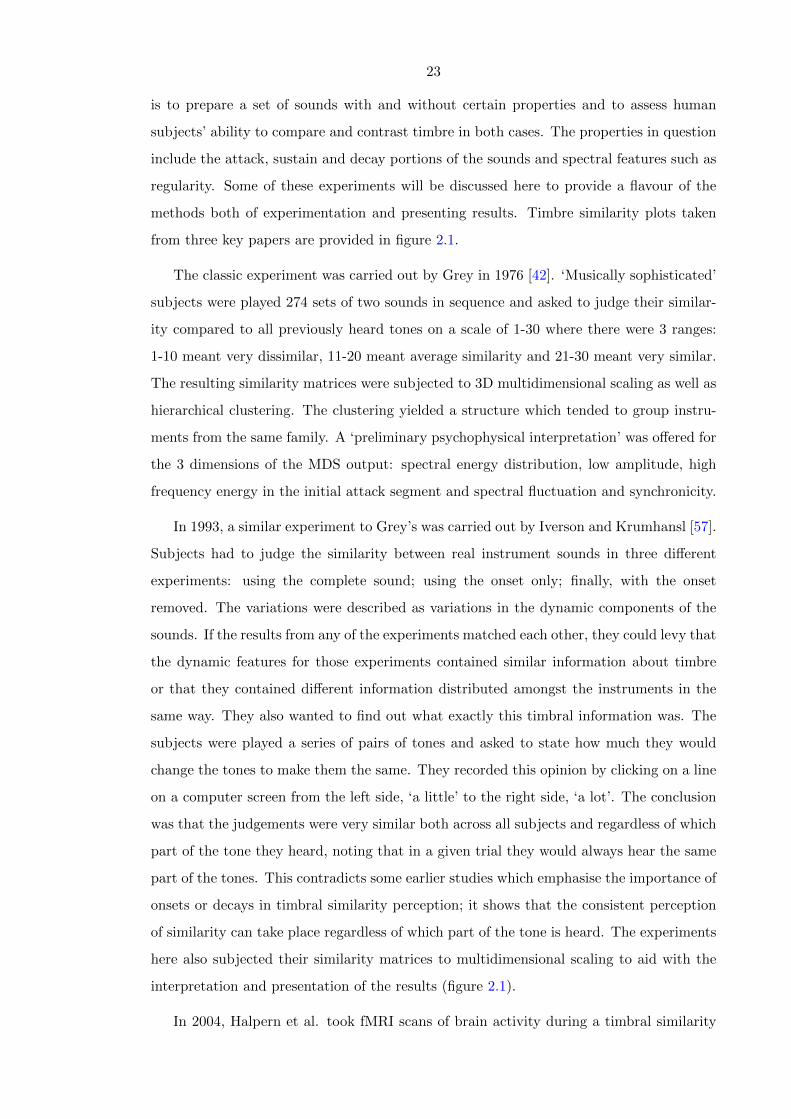
23

is to prepare a set of sounds with and without certain properties and to assess human

subjects’ ability to compare and contrast timbre in both cases. The properties in question

include the attack, sustain and decay portions of the sounds and spectral features such as

regularity. Some of these experiments will be discussed here to provide a flavour of the

methods both of experimentation and presenting results. Timbre similarity plots taken

from three key papers are provided in figure 2.1.

The classic experiment was carried out by Grey in 1976 [42]. ‘Musically sophisticated’

subjects were played 274 sets of two sounds in sequence and asked to judge their similar-

ity compared to all previously heard tones on a scale of 1-30 where there were 3 ranges:

1-10 meant very dissimilar, 11-20 meant average similarity and 21-30 meant very similar.

The resulting similarity matrices were subjected to 3D multidimensional scaling as well as

hierarchical clustering. The clustering yielded a structure which tended to group instru-

ments from the same family. A ‘preliminary psychophysical interpretation’ was offered for

the 3 dimensions of the MDS output: spectral energy distribution, low amplitude, high

frequency energy in the initial attack segment and spectral fluctuation and synchronicity.

In 1993, a similar experiment to Grey’s was carried out by Iverson and Krumhansl [57].

Subjects had to judge the similarity between real instrument sounds in three different

experiments: using the complete sound; using the onset only; finally, with the onset

removed. The variations were described as variations in the dynamic components of the

sounds. If the results from any of the experiments matched each other, they could levy that

the dynamic features for those experiments contained similar information about timbre

or that they contained different information distributed amongst the instruments in the

same way. They also wanted to find out what exactly this timbral information was. The

subjects were played a series of pairs of tones and asked to state how much they would

change the tones to make them the same. They recorded this opinion by clicking on a line

on a computer screen from the left side, ‘a little’ to the right side, ‘a lot’. The conclusion

was that the judgements were very similar both across all subjects and regardless of which

part of the tone they heard, noting that in a given trial they would always hear the same

part of the tones. This contradicts some earlier studies which emphasise the importance of

onsets or decays in timbral similarity perception; it shows that the consistent perception

of similarity can take place regardless of which part of the tone is heard. The experiments

here also subjected their similarity matrices to multidimensional scaling to aid with the

interpretation and presentation of the results (figure 2.1).

In 2004, Halpern et al. took fMRI scans of brain activity during a timbral similarity

24

Figure 2.1: Different plots of human similarity judgements, derived by performing MDS on similarity

matrices. Top taken from Grey 1976 [42], middle taken from Iverson and Krumhansl 1993

[57] and bottom taken from Halpern et al. 2004 [43].

25

experiment. The subjects judged timbral similarity using a 5 button response pad, where

1 signified ‘high similarity’ and 5 ‘low similarity’ [43]. Since this study was concerned

not merely with timbral similarity, but also with the areas of the brain involved in the

imagining of timbre, subjects had to compare sounds they had actually heard as well as

comparing sounds they imagined. This provided two sets of results, which were subjected

to 2D multidimensional scaling and plotted. They define the two axes of the plot as

brilliance and nasality, terms derived from an earlier study by Kendall et al. [63]. For

example, the oboe is ‘nasal and brilliant’, the tenor sax is ‘nasal and not brilliant’.

Terasawa et al. worked in the opposite direction from some other studies: starting

with a numerical description of timbral space, they validated that description using lis-

tener similarity judgements [121]. They described timbre space as the space of possible

13 dimensional Mel Frequency Cepstra (MFC) or Linear Frequency Cepstra (LFC) coef-

ficients. They sampled sparsely and uniformly in two dimensions of that space at a time

and then re-synthesized audio from the MFCCs/ LFCCs. Listeners were asked to judge

the similarity between sounds derived from reference points in the space to sounds from

random points in the space on a scale of 1 to 10 (identical to very different). Thus they

were able to assess if the similarity varied smoothly from one point in the space to another.

The results support the use of the mel scale over the linear scale and show that MFCCs

can be used to explain 66% of the perceived variation in timbre. The researchers conclude

as follows:

This result is interesting because we have ... established that MFCC parame-

ters are a good perceptual representation for static sounds.

The researchers considered static sounds to be sounds where the spectrum does not

change over time. Is this a reasonable description of real instrument timbres? Is it valid

to construct systems that deal with isolated snapshots of instrument timbres? The work

of Terasawa et al. suggests that sufficient information can be transmitted in a static tone

to enable a human to effectively judge similarity. Humans do not need spectral dynamics

to differentiate timbres.

2.3 The Ideal Numerical Representation of Timbre

In this section, the perceptual and computational considerations for an ideal numerical

representation of timbre are discussed.

If we consider the description of the ascending auditory pathway presented above along

26

with the various parts of the perceptual picture that are provided by the listener based

experiments, what conclusions can be drawn about the ideal representation of timbre for

the purposes of guiding an optimisation algorithm through sound synthesis space?

The perceptual considerations are as follows:

1. It should take account of the multidimensional nature of timbre.

2. It should take account of the non linear frequency scale observed in the perception

of pitch.

3. It should take account of the logarithmic nature of amplitude perception.

4. It should be able to measure perceptually important features such as brightness and

nasality.

5. It should be reasonably orthogonal (i.e. decorrelated) within itself, to ensure a

compact representation.

6. It should offer a smooth transition from one point in the timbral space to another.

This is a practical consideration that will be required for search-type optimisers such

as those investigated in chapter 3.

The computational considerations are as follows:

1. Is should already exist in a library form, or at least parts of the process of extraction

should.

2. It should be well described to enable new implementations.

3. It should be computationally efficient for the purposes of extraction and comparison

across large databases of sounds.

2.4 The MFCC Feature

The Mel Frequency Cepstrum Coefficient or MFCC was originally used for the purposes of

speech recognition, as reported in 1980 by Davis and Mermelstein [31], where it was used

as a compact way of representing the salient features of the spectral envelope of speech

signals. The combination of ideas that make up the MFCC are also to be found in a 1976

paper by Mermelstein [84]. The Mel scale was first described in a 1937 paper by Stevens

et al. [116]. There are other perceptual scales such as the Bark scale but the Mel scale is

considered sufficiently accurate, evidenced by a large body of research using it. According

27

sample time domain signal

extract complex spectrum

take log of amplitude spectrum

pass spectrum through mel filter bank

take the DCT of the filter bank outputs

Figure 2.2: An overview of the process of extracting an MFCC feature vector from a time domain signal.

to Rabiner and Schafer [100], the term cepstrum was coined, along with several other new

words, by Bogert et al. in a classic paper entitled ‘The quefrency alanysis of time series

for echoes: Cepstrum, Pseudo-Autocovariance, Cross-Cepstrum and Saphe Cracking’ [10].

Rabiner and Juang provide an extensive comparative description of the design of features

for speech recognition, including the MFCC [99, p. 163-190].

The following subsections contain a detailed description and justification of the MFCC,

a comparison of current open source implementations of MFCC extractors and a descrip-

tion of a new Java MFCC extractor.

2.4.1 Extracting MFCCs

MFCCs are extracted via a series of transformations and distortions which will now be

described within the perceptual framework from the previous sections. An overview of the

MFCC feature extraction process is provided in figure 2.2 and a comparison of the Mel

frequency scale to the equal temperament scale (as represented by midi note numbers) is

provided in figure 2.3.

The analog signal is sampled into the digital domain such that the subsequent steps

can be ‘mechanised’. The complex spectrum is taken, after the ‘bank-of-filters’ speech

recognition system front-end from [99, p. 81-84], wherein it is stated that ‘probably the

most important parametric representation of speech is the short time spectral envelope.’.

Following this, the logarithm of the magnitude spectrum is taken, motivated by the

widely accepted fact that the perception of loudness is logarithmic, e.g. the dB scale. This

is another impact of the human perceptual apparatus on the design of the feature vector.

Next, the frequency scale of the magnitude spectrum is warped using the Mel frequency

scale. The Mel scale is derived from studies of the human perception of pitch [116]; the

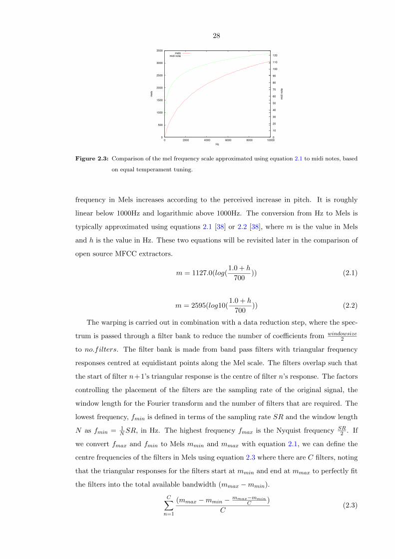
28

0

500

1000

1500

2000

2500

3000

3500

0 2000 4000 6000 8000 10000

0

10

20

30

40

50

60

70

80

90

100

110

120

me

ls

mid

i n

ote

Hz

mels

midi note

Figure 2.3: Comparison of the mel frequency scale approximated using equation 2.1 to midi notes, based

on equal temperament tuning.

frequency in Mels increases according to the perceived increase in pitch. It is roughly

linear below 1000Hz and logarithmic above 1000Hz. The conversion from Hz to Mels is

typically approximated using equations 2.1 [38] or 2.2 [38], where m is the value in Mels

and h is the value in Hz. These two equations will be revisited later in the comparison of

open source MFCC extractors.

m = 1127.0(log(1.0 + h

700)) (2.1)

m = 2595(log10(1.0 + h

700)) (2.2)

The warping is carried out in combination with a data reduction step, where the spec-

trum is passed through a filter bank to reduce the number of coefficients from windowsize2

to no.filters. The filter bank is made from band pass filters with triangular frequency

responses centred at equidistant points along the Mel scale. The filters overlap such that

the start of filter n+1’s triangular response is the centre of filter n’s response. The factors

controlling the placement of the filters are the sampling rate of the original signal, the

window length for the Fourier transform and the number of filters that are required. The

lowest frequency, fmin is defined in terms of the sampling rate SR and the window length

N as fmin = 1N SR, in Hz. The highest frequency fmax is the Nyquist frequency SR

2 . If

we convert fmax and fmin to Mels mmin and mmax with equation 2.1, we can define the

centre frequencies of the filters in Mels using equation 2.3 where there are C filters, noting

that the triangular responses for the filters start at mmin and end at mmax to perfectly fit

the filters into the total available bandwidth (mmax −mmin).

C∑n=1

(mmax −mmin − mmax−mminC )

C(2.3)

29

To summarise at this point, the output of the Mel filter bank can be described as

a low dimensional, perceptually weighted log magnitude spectrum, containing typically

up to 42 coefficients. The final stage of the MFCC extraction is to perform a further

transform on the outputs of the filter bank. The results of this are cepstral coefficients,

so called because they are the transform of a transform; ‘spec’ becomes ‘ceps’. Different

types of transforms could be used to create cepstral coefficients from the output of the

filter bank but the favoured transform is the Discrete Cosine Transform (DCT). The DCT

is commonly used in digital signal processing as a stage in encoding signals for efficient

storage or transmission, e.g. the JPEG image compression format. A tutorial can be

found in [65]. The role of the DCT in the MFCC extraction is to enable source and filter

separation as well as further compression of the representation of the signal. It has certain

interesting properties which make it appropriate for these tasks: it decorrelates the signal

and it redistributes the information towards the lower coefficients.

Decorrelating the signal in this case means it reduces the linkage or covariance between

separate values in the original signal. From the speech synthesis perspective, this is said to

separate the source and channel, i.e. the larynx and the ‘band pass filters’ of the mouth.

This leads to a speaker independent characteristic, where the focus is on the positions of

the band pass filters, not the signal flowing through them. In terms of musical instruments,

this makes it useful for recognising the distinctive timbre of a note, regardless of what was

used to make it as the variations caused by pitch should be removed. It is well established

that the MFCC is useful for representing the salient aspects of the spectrum for speech

recognition but in [66] the researchers report that the MFCC is ineffective for speaker

recognition. In terms of musical instruments, this could be interpreted as being unable to

guess the source (violin or cello string) but being able to tell the difference between the

filter (the body of the instrument).

A further aspect of the decorrelation of the signal is that it makes it less meaningful to

compare different coefficients to each other, e.g. coefficient 1 from sound 1 to coefficient 2

from sound 2, which makes it possible to use a simple distance metric.

Redistributing the information towards the lower coefficients means the higher coef-

ficients can be discarded and a close representation of the signal is still retained. This

makes the representation compact. This makes it similar to the more complex transform

used in Principle Component Analysis, the Karhunen-Loeve transform, which is perhaps

less popular due to its complexity, despite superior performance [112, p. 496]. In other

words, using the DCT approximates PCA.

30

For a more mathematical description of the MFCC, the reader is referred to Rabiner

and Juang [99, p. 163-190].

2.4.2 MFCCs for Music Orientated Tasks

Whilst the majority of applications of the MFCC have been to the problem of speech

recognition, its use for instrument recognition and Music Information Retrieval (MIR)

systems has been multifarious. Logan provides a well cited and convincing justification

for the use of the MFCC in musical modelling, supporting the use of the warped frequency

scale and the Discrete Cosine Transform [74]. Casey et al. provide an overview of the

state of the art of content based MIR circa 2008; the use of the MFCC is promoted for

the purposes of timbral description [16]. Eronen shows that the MFCC is the best single

feature in a comparison of features for music instrument recognition [33]. A comparison to

a listener experiment ground truth is also provided where the MFCC appears to correlate

surprisingly well with listener judgement in terms of the ‘confusion matrix’. Brown et

al. present a study where cepstral coefficients prove to be the most effective for a wood-

wind instrument recognition task, suggesting that they are also effective for differentiation

within a confined set of timbres (oboe, sax, flute, and clarinet in this case) [14]. In sum-

mary, the MFCC has been widely used and validated as a numerical measure of musical

instrument timbre.

2.4.3 Open Source MFCC Implementations

In order to carry out some of the work reported later in this thesis, it was necessary to

find an efficient and batch-processing capable way to extract MFCCs from time domain

audio signals. An existing library or module could be used or a new implementation could

be created. An initial survey of existing MFCC implementations provided a variety of

options but also posed questions about the details of MFCC implementation and what

was the best particular implementation for the timbral comparison task.

There have been previous comparisons of MFCC extraction implementations, but they

are speech not timbre focused. Ganchev et al. carried out a comparison of several available

implementations circa 2005 for the speaker verification task [38]. This provides an insight

into some of the properties of the MFCC that tend to vary, namely the frequency response

and the number and placement of filters in the filter bank. Zheng et al. implement an

MFCC extractor and vary the frequency response curves and overlapping of filters in the

filter bank [147]. They then analyse the performance against a standard Mandarin speech

31

recognition database. They conclude that the shape of the frequency responses does not

make a large difference but the overlapping thereof has a positive effect on recognition

performance.

For this study, the following open source MFCC extractors were compared: Super-

Collider3’s MFCC UGen [25], the MFCC and associated classes from the Beads Java

computer music system [12], the MFCC and associated classes from the CoMIRVA Java

toolkit [106] and the xtract mfcc and associated functions from the libxtract C feature

extraction library [15]. This is not an exhaustive list of open source MFCC implementa-

tions, but it provides an insight into the typical variation between implementations since

each implementation has quite a different context in terms of language or application.

Considering the applications discussed in this thesis, the SuperCollider environment is

used directly, Beads is an environment that was originally conceived for the construction

of live algorithms and interactive music systems and the other two extractors were de-

signed partly for Music Information Retrieval purposes. This choice of MFCC extractors

therefore intersects strongly with the areas in which the work discussed in this thesis is sit-

uated. Other open source MFCC extractor implementations include jAudio [81], Marsyas

[58] and Sphix-4 [129]. The four extractors are compared at the implementation level then

their performance at a timbral similarity task is compared.

2.4.4 An Implementation-level Comparison of Open Source MFCC ex-

tractors

The implementation level comparison was carried out via an examination of the source

code of the MFCC extractors. The extractors were compared in terms of their time domain

processing, filter banks and Discrete Cosine Transform implementations.

Time Domain Signal Processing

The first difference observed was in the treatment of the time domain signal, where the

CoMIRVA toolkit differed by its use of normalisation of the signal x at time n using

equation 2.4. The motivation for this is stated in the source code as ‘rescaling the input

samples ... to 96dB’.

x[n] = x[n].109620 (2.4)

The other systems used the raw time domain data.

32

Filter Banks

All of the systems pre-calculate coefficients for the filter bank transformation for efficiency.

However, there is a variation in the number of filters used in the filter bank as well as the

number of DCT coefficients generated subsequently. The CoMIRVA system defaults to

20 coefficients generated from 40 filters, but the programmer using this API can change

this. The Beads system has no default for the number of filters or coefficients. The

SuperCollider3 implementation uses 42 filters and produces up to 42 coefficients, with a

default of 13 coefficients. The libxtract library has no default for either parameter. The

frequency ranges within which the filters are placed also vary: CoMIRVA defaults to 20-

16000Hz but can be changed, Beads has a hard limit of 8000Hz, SuperCollider3 always

uses 80-18000Hz and libxtract has no defaults or limits (beyond those imposed by the

sampling theorem).

The final variation in the filter bank set up is the way that the output of the filters is

perceptually scaled prior to the DCT. Equations 2.5, 2.6, 2.7 and 2.8 illustrate this scaling

for CoMIRVA, Beads, SuperCollider3 and libxtract where yn is the output from a given

filter bank. These functions are plotted in figure 2.4. The shapes of the curves are the

same but the units are different.

log(yn) (2.5)

max(0, 10 log(yn

log(10)) (2.6)

10(log 10(yn) + 5) (2.7)

max(log(yn), 2(10−42)) (2.8)

DCT Calculation

The extractors also vary in their calculation of the DCT. They all pre-calculate a matrix

of DCT coefficients of the appropriate size for the number of filters and the number of

MFCCs required, but they do so in different ways. Equations 2.9, 2.10 and 2.11 show how

this is done in CoMIRVA, Beads and SuperCollider3, where b is the number of filters, N

is the number of MFCCs, k = 0, 1..., b− 1 and n = 0, 1..., N − 1. libxtract uses the DCT

provided by the fftw library [36]. √2

bcos(

π

bk(n+ 0.5)) (2.9)

33

0

0.5

1

1.5

2

2.5

3

3.5

4

4.5

5

0 20 40 60 80 100

log(x)

-10

-5

0

5

10

15

20

25

30

35

40

0 20 40 60 80 100

(10 * log(x/log(10)))

50

52

54

56

58

60

62

64

66

68

70

0 20 40 60 80 100

10 * (log10(x) + 5)

0

0.5

1

1.5

2

2.5

3

3.5

4

4.5

5

0 20 40 60 80 100

log(x)

Figure 2.4: Perceptual scaling functions used for the different feature extractors. Clockwise from the top

left: CoMIRVA, Beads, SuperCollider3 and libxtract.

√2

bcos(

π(n+ 1)(k + 0.5)

b) (2.10)

cos(π

b(n+ 0.5)(k + 1)) (2.11)

The above analysis shows that there is variation between MFCC extractors in terms

of their filter bank and DCT implementations but there is also variation in the way that

they can be used. Beads is designed to run as a realtime computer music system and

does not currently support an offline batch mode. SuperCollider3 is also mainly designed

to run in real time but does support non realtime operation. CoMIRVA and libxtract

are perhaps more suited to batch processing tasks but CoMIRVA provides a much more

complex feature set than was required for the work here and libxtract was not written in

the author’s preferred prototyping language (Java). So a novel, as simple as possible Java

implementation was made and subsequently made available under an open source license

[141]. This is briefly discussed in the final part of this section.

2.4.5 A Performance Comparison of the MFCC Extractors

To assess the performance of the MFCC extractors, they were compared in their ability

to judge timbral similarity in a controlled scenario. A simple FM synthesis algorithm

with a single parameter was implemented. The parameter, the modulation index, was

varied from zero up to a maximum value in 100 steps and 100 audio files containing the

34

0

20

40

60

80

100

0 10 20 30 40 50 60 70 80 90 100

MF

CC

dis

tan

ce

Parametric distance

Beads MFCC Distance Against Parametric Variation

0

20

40

60

80

100

0 10 20 30 40 50 60 70 80 90 100

MF

CC

dis

tan

ce

Parametric distance

COMIRVA MFCC Distance Against Parametric Variation

0

20

40

60

80

100

0 10 20 30 40 50 60 70 80 90 100

MF

CC

dis

tan

ce

Parametric distance

libxtract MFCC Distance Against Parametric Variation

0

20

40

60

80

100

0 10 20 30 40 50 60 70 80 90 100

MF

CC

dis

tan

ce

Parametric distance

SuperCollider3 MFCC Distance Against Parametric Variation

Figure 2.5: Normalised distances from a reference sound to each of the other sounds. The reference sound

has index 0. The linear plot included shows the expected distance if distance in feature space

correlates with distance in parameter space.

synthesizer’s output were written to disk, one for each parametric variation. The MFCC

extractors were used to calculate MFCC vectors for each of the 100 sound files; distance

matrices from each vector to each other vector were computed; finally distances from each

vector to the vector for the first sound were computed. There are two main aims here:

to establish if the extractors could expose the underlying process of parametric variation

and to compare the values generated by the different extractors.

Exposing the Underlying Process of Parametric Variation

Figure 2.5 shows the normalised distances from each of the 100 sounds to the first sound.

As the sound index increases, the parameter setting also increases. If distance in MFCC

feature space correlates to distance in parameter space, the line should follow the linear

reference line shown on the graphs. It does not which, as suggested by the full distance

matrices in figure 2.6, means the perceptual distance from the reference sound to the other

sounds varies in a non-linear fashion. It is important to note that two sounds that are

equidistant from a reference sound in feature space will not necessarily be close to each

other. They may be in completely different positions in feature space, positions which

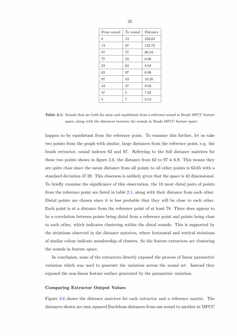
35

From sound To sound Distance

6 13 232.64

13 87 132.73

87 77 96.34

77 23 6.00

23 62 8.94

62 97 6.96

97 43 18.20

43 47 9.02

47 5 7.92

5 7 8.53

Table 2.1: Sounds that are both far away and equidistant from a reference sound in Beads MFCC feature

space, along with the distances between the sounds in Beads MFCC feature space.

happen to be equidistant from the reference point. To examine this further, let us take

two points from the graph with similar, large distances from the reference point, e.g. the

beads extractor, sound indexes 62 and 97. Referring to the full distance matrices for

these two points shown in figure 2.6, the distance from 62 to 97 is 6.9. This means they

are quite close since the mean distance from all points to all other points is 63.65 with a

standard deviation 47.28. This closeness is unlikely given that the space is 42 dimensional.

To briefly examine the significance of this observation, the 10 most distal pairs of points

from the reference point are listed in table 2.1, along with their distance from each other.

Distal points are chosen since it is less probable that they will be close to each other.

Each point is at a distance from the reference point of at least 78. There does appear to

be a correlation between points being distal from a reference point and points being close

to each other, which indicates clustering within the distal sounds. This is supported by

the striations observed in the distance matrices, where horizontal and vertical striations

of similar colour indicate membership of clusters. So the feature extractors are clustering

the sounds in feature space.

In conclusion, none of the extractors directly exposed the process of linear parametric

variation which was used to generate the variation across the sound set. Instead they

exposed the non-linear feature surface generated by the parametric variation.

Comparing Extractor Output Values

Figure 2.6 shows the distance matrices for each extractor and a reference matrix. The

distances shown are sum squared Euclidean distances from one sound to another in MFCC

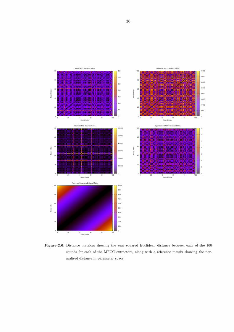
36

0

20

40

60

80

100

0 20 40 60 80 100

So

un

d in

de

x

Sound index

Beads MFCC Distance Matrix

’./TestFMOSbeads_distance_matrix.txt’

0

50

100

150

200

250

300

350

0

20

40

60

80

100

0 20 40 60 80 100

So

un

d in

de

x

Sound index

COMIRVA MFCC Distance Matrix

’./TestFMOScomirva_distance_matrix.txt’

0

5000

10000

15000

20000

25000

30000

35000

40000

0

20

40

60

80

100

0 20 40 60 80 100

So

un

d in

de

x

Sound index

libxtract MFCC Distance Matrix

’./TestFMOSlibxtract_distance_matrix.txt’

0

100000

200000

300000

400000

500000

600000

0

20

40

60

80

100

0 20 40 60 80 100

So

un

d in

de

x

Sound index

SuperColldier3 MFCC Distance Matrix

’./TestFMOSsc_distance_matrix.txt’

0

2

4

6

8

10

12

14

0

20

40

60

80

100

0 20 40 60 80 100

So

un

d in

de

x

Sound index

Reference Parametric Distance Matrix

’./TestFMOSreference_distance_matrix.txt’

0

1000

2000

3000

4000

5000

6000

7000

8000

9000

10000

Figure 2.6: Distance matrices showing the sum squared Euclidean distance between each of the 100

sounds for each of the MFCC extractors, along with a reference matrix showing the nor-

malised distance in parameter space.

37

beads comirva libxtract SC3 ref

beads 1 0.635359023 0.06984181 0.71293421 0.0481178381

comirva 1 0.07026185 0.72980517 0.0284692813

libxtract 1 0.10615515 -0.0644420928

SC3 1 0.0343739248

ref 1

Table 2.2: Pearson’s correlations between the distance matrices for each MFCC extractor and the refer-

ence matrix.

space, or in parameter space for the reference matrix. The reference matrix shows the

expected result if distance in parameter space correlates linearly with distance in timbre

space. The matrices are very different from the reference matrix but less so from each

other. Some parametric settings produce sounds which are close to several other sounds:

observe the distance of sound 38 to other sounds in the COMIRVA plot, where several

points have similarly low distances.

So the extractors do not agree with the reference matrix, but do they agree with

each other? Table 2.2 shows the Pearson’s correlations between the four MFCC distance

matrices and the reference matrix. The correlation between COMIRVA, SuperCollider3

and Beads is very significant. The correlation with libxtract is very low by comparison;

Libxtract disagrees significantly with the other extractors as to the distance between the

100 sounds in MFCC feature space. This could be explained as an error in the method

used to produce the libxtract MFCCs or as a significant difference in the implementation.

The examination of source code in the previous section did not indicate any obvious major

difference, so it is thought that the difference is due to a flaw elsewhere in the tool chain.

To conclude the comparison of MFCC extractors, there are variations in the imple-

mentations in their placement of filter banks and use of the DCT. This results in widely

varying output values. Once normalised though, the correlation between the outputs of 3

out of 4 of the extractors is very significant. This correlation is expected given that they

do not vary hugely in their implementations. The libxtract extractor, which did not cor-

relate well with the others, was most likely not used properly but it is not clear where the

issue was. Finally, the feature extractors do not seem to be able to uncover an underlying

linear variation in a parameter in the test synthesizer used here. This shows that linear

movement in parameter space results in non-linear movement in feature space. Perhaps

the non linearity of feature space as defined by the variation of even a single parameter

is part of what makes synthesizer programming difficult. The difficulty of programming a

38

synthesizer is addressed further in section 4.1.1.

2.4.6 Novel MFCC Extractor Implementation

An MFCC feature extractor was made in Java, optimised for code portability and ease of

use in batch processing. The power spectrum is extracted; the Mel filter bank output is

calculated using triangular frequency responses, where the user selects the range within

which the filters are placed and the number of filters; the log of the filter output is taken

using equation 2.5; and finally a DCT is applied using equation 2.9 to produce the number

of coefficients requested by the user. The implementation was carried out prior to a full

examination of the CoMIRVA implementation and is based on the literature but it ended

up being essentially the same. Its main raison d’etre is that it is much simpler to deploy

in a new project due to its simplistic, two class organisation. In the following section, a

system which uses the MFCC extractor along with dimensional reduction to allow rapid

exploration of sound synthesis space is described.

2.5 Presenting Timbre Similarity: SoundExplorer

In this section, some original work is presented where MFCC feature vectors are used along

with Multidimensional Scaling to construct a sound exploration tool, ‘SoundExplorer’.

SoundExplorer allows the user to explore a high dimensional sound synthesis space using

a two dimensional interface. The tool aims to solve the problem that sound synthesis

algorithms have many parameters and that this makes it difficult or impossible for a user to

fully explore the range of sounds that synthesizer can make. Some might not consider this

a problem; part of the creative process is exploration, after all; but what if the exploration

could be made more complete and focused? That way, the creative, exploratory phase

is retained yet the search carried out therein might be more comprehensive, potentially

yielding better results. Consider a typical sound synthesizer interface, such as the ‘knobs

and sliders’ based example found on a Moog synthesizer. This is an old interface paradigm

but it is alive and well in virtual synthesizers, as a quick perusal of the virtual synthesizer

database available at KVR audio will show [53]. How does the user interact with this

interface? The reader is referred to a later section (4.4.2) where the behaviour of human

synthesizer programmers is analysed in more detail, but the upshot is that the user tends

to focus on one or two parameters at a time. The reason for this is beyond the scope of

this work but is presumably due to physical and/ or mental limitations.

There are two approaches to solving this problem: to concoct a mapping from two

39

or three meta parameters to many more parameters or to provide some other means of

reducing the dimensionality of synthesizer control. The former approach is exemplified by

such systems as Bencina’s ‘Metasurface’. Metasurface provides a two dimensional space

for exploration by the user that is mapped to a higher dimensional parameter space by

means of a parametric interpolation technique. In essence, points are defined in a 2D space

and attached to the points are particular, high dimensional parameter settings or presets.

The user chooses coordinates in the space and interpolation is carried out between the

presets located nearby to the user’s chosen coordinate to provide a preset for their chosen

position [7]. A summary of related work is also provided in Bencina’s paper. What is

the motivation for the second method of dimensional reduction, where the parameters are

ignored in the dimensional reduction?

The work analysing MFCC output in the previous section indicates that closeness of

parameter setting does not necessarily equate to closeness of timbre, at least as measured

by an MFCC feature. This is true even for a simple, single parameter synthesizer. So there

is a potentially flawed assumption in parameter based systems such as Metasurface and

indeed any interface permitting direct parametric manipulation that parametric distance

correlates with timbral distance. One alternative to a parameter-based system is a timbre-

based system, where timbre features are used to represent the sounds and the dimensional

reduction is carried out on the timbral features. Proximity in these systems implies timbral

as opposed to parametric similarity. Recent prior work here is Stowell’s work mapping

vocal features to sound synthesizer parameters with self organising maps [117]. Sound-

Explorer was partly visually inspired by Schwarz’s work on the CataRT system, which

presents a corpus of musical material in a 2D space, arranged according to audio feature

proximity [108]. This system then generates new material using concatenative resynthe-

sis. SoundExplorer differs in that it synthesizes its output at the synthesis parameter level

as opposed to using a corpus of pre-existing sounds. Here follows a description of the

SoundExplorer tool.

SoundExplorer allows the user to interactively explore the space of possible sounds for

a synthesis algorithm or any set of audio files by clicking on items in a 2D space. The

relative positions of the items in the space are calculated by the MDS algorithm such that

the distances between the points in the low dimensional space approximate the distances

in the higher dimensional space between the original feature vectors [41]. Points that are

close together in the 2D space should therefore sound similar.

The motivation for the construction of this tool was firstly to gain an insight into the

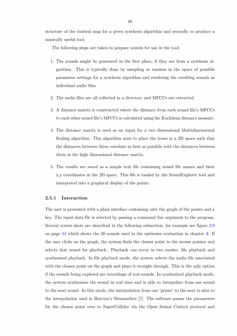
40

structure of the timbral map for a given synthesis algorithm and secondly to produce a

musically useful tool.

The following steps are taken to prepare sounds for use in the tool:

1. The sounds might be generated in the first place, if they are from a synthesis al-

gorithm. This is typically done by sampling at random in the space of possible

parameter settings for a synthesis algorithm and rendering the resulting sounds as

individual audio files.

2. The audio files are all collected in a directory and MFCCs are extracted.

3. A distance matrix is constructed where the distance from each sound file’s MFCCs

to each other sound file’s MFCCs is calculated using the Euclidean distance measure.

4. The distance matrix is used as an input for a two dimensional Multidimensional

Scaling algorithm. This algorithm aims to place the items in a 2D space such that

the distances between them correlate as best as possible with the distances between

them in the high dimensional distance matrix.

5. The results are saved as a simple text file containing sound file names and their

x,y coordinates in the 2D space. This file is loaded by the SoundExplorer tool and

interpreted into a graphical display of the points.

2.5.1 Interaction

The user is presented with a plain interface containing only the graph of the points and a

key. The input data file is selected by passing a command line argument to the program.

Several screen shots are described in the following subsection, for example see figure 2.9

on page 44 which shows the 20 sounds used in the optimiser evaluation in chapter 3. If

the user clicks on the graph, the system finds the closest point to the mouse pointer and

selects that sound for playback. Playback can occur in two modes: file playback and

synthesized playback. In file playback mode, the system selects the audio file associated

with the chosen point on the graph and plays it straight through. This is the only option

if the sounds being explored are recordings of real sounds. In synthesized playback mode,

the system synthesizes the sound in real time and is able to interpolate from one sound

to the next sound. In this mode, the interpolation from one ‘preset’ to the next is akin to

the interpolation used in Bencina’s Metasurface [7]. The software passes the parameters

for the chosen point over to SuperCollider via the Open Sound Control protocol and

41

Key Instrument Key Instrument Key Instrument

0 Cello att 7 Piano sus 14 Horn att

1 Piano att 8 Alto flute sus 15 Alto sax sus

2 Violin att 9 Bassoon sus 16 Alto sax att

3 Bassoon att 10 B[ 17 Oboe sus

clarinet sus

4 Trumpet sus 11 Oboe att 18 B[

clarinet att

5 Cello sus 12 Alto flute att 19 Horn sus

6 Violin sus 13 Trumpet att

Table 2.3: This table shows the indices used for the synth vs. real instrument plots in figures 2.8 and

2.10.

SuperCollider passes them to a running synthesizer. A final feature of the software is the

zoom feature, which allows the user to zoom into the graph. This is useful considering

that there may be many thousands of points quite close to each other.

2.5.2 Graphical Output

The synthesis algorithms used in this section are described in detail in the following chap-

ter, section 3.1. In summary, BasicFMOS is a 2 parameter FM synthesizer with two

oscillators in a modulator-carrier pair; interFMOS is a 22 parameter, three oscillator FM

synthesizer with variable modulation routing; BasicSubOS is a basic 3 parameter sub-

tractive synthesizer; InterSubOS is a more complex, 17 parameter subtractive synthesizer.

The instruments used are the same 10 used in the following chapter, namely Alto Flute,

Alto Sax, Bassoon, B[ Clarinet, Cello, French Horn, Oboe, Piano, Trumpet and Violin.

In some of the following images, the instruments are labelled numerically using the indices

from table 2.3.

The images are quite fascinating in their own right. Exploring the images sonically

allows the user to engage with the sound synthesis algorithm in a quite novel way. To

briefly analyse the images. The BasicFMOS synthesizer uses a strongly quantised param-

eter, which explains the web like structure. Each strand represents a different point along

the quantised parameter’s range. The other images are more difficult to interpret. The

real instruments seem to integrate best with the InterFMOS synthesizer, in that they are

clearly very close to many of its timbral points. This indicates that this synthesizer should

be effective at re-synthesizing the real instrument sounds, a question which is addressed

much more conclusively in the chapter 3. The real instruments did not seem to map into

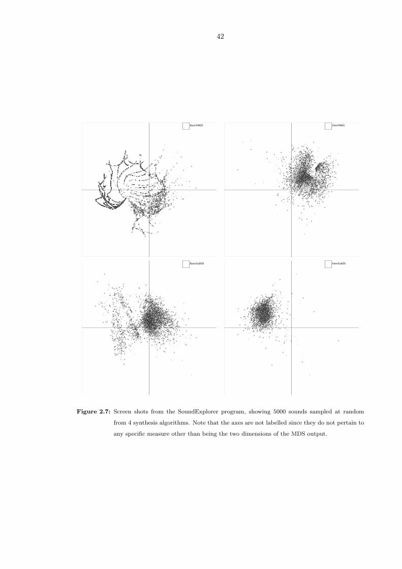
42

Figure 2.7: Screen shots from the SoundExplorer program, showing 5000 sounds sampled at random

from 4 synthesis algorithms. Note that the axes are not labelled since they do not pertain to

any specific measure other than being the two dimensions of the MDS output.

43

Figure 2.8: Screen shots from the SoundExplorer program showing 5000 random sounds from each synth

plotted against the 20 acoustic instrument sounds. Note that the axes are not labelled since

they do not pertain to any specific measure other than being the two dimensions of the MDS

output.

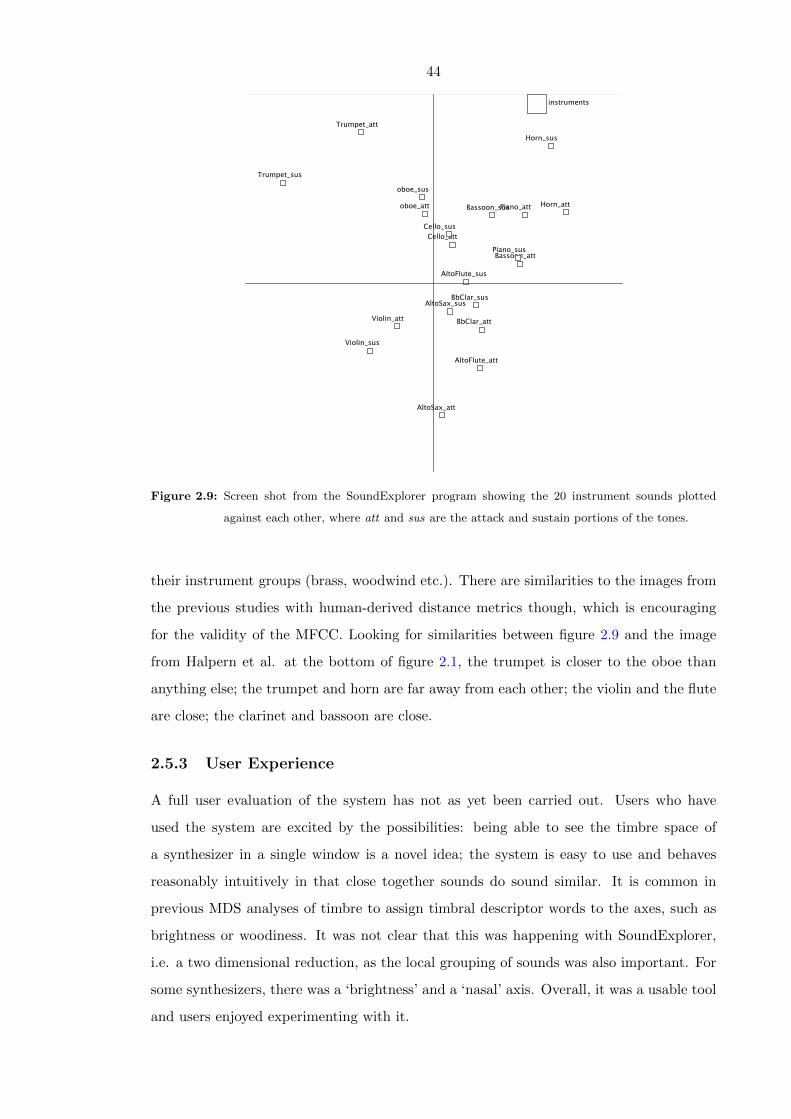
44

Figure 2.9: Screen shot from the SoundExplorer program showing the 20 instrument sounds plotted

against each other, where att and sus are the attack and sustain portions of the tones.

their instrument groups (brass, woodwind etc.). There are similarities to the images from

the previous studies with human-derived distance metrics though, which is encouraging

for the validity of the MFCC. Looking for similarities between figure 2.9 and the image

from Halpern et al. at the bottom of figure 2.1, the trumpet is closer to the oboe than

anything else; the trumpet and horn are far away from each other; the violin and the flute

are close; the clarinet and bassoon are close.

2.5.3 User Experience

A full user evaluation of the system has not as yet been carried out. Users who have

used the system are excited by the possibilities: being able to see the timbre space of

a synthesizer in a single window is a novel idea; the system is easy to use and behaves

reasonably intuitively in that close together sounds do sound similar. It is common in

previous MDS analyses of timbre to assign timbral descriptor words to the axes, such as

brightness or woodiness. It was not clear that this was happening with SoundExplorer,

i.e. a two dimensional reduction, as the local grouping of sounds was also important. For

some synthesizers, there was a ‘brightness’ and a ‘nasal’ axis. Overall, it was a usable tool

and users enjoyed experimenting with it.

45

Figure 2.10: Screen shot from the SoundExplorer program showing 1000 sounds from each synth plotted

together with the 20 instrument sounds. Note that the axes are not labelled since they

do not pertain to any specific measure other than being the two dimensions of the MDS

output.

46

2.6 Summary

The ascending auditory pathway has been described along with the limitations and quirks

of the mammalian perceptual hardware. The kinds of data modelling observed in the

auditory pathway have been discussed in order to establish the validity of a spectrally

derived measure of timbre. The question ‘what is timbre?’ has been asked and answers

derived from a variety of sources, including several decades of listener based experiments.

The features of an ideal numerical measure of timbral similarity have been tentatively

suggested. The history and widespread use of the MFCC has been discussed and the

perceptual grounds for its design has been provided. Several open source implementations

of MFCC extractors have been compared and a simple, new implementation has been

introduced. Finally, a new tool has been described which allows its user to interactively

explore high dimensional timbre spaces which have been mapped into a two dimensional

space using multidimensional scaling.

In the following chapter, a shift is made from observations and representations of

timbre space to the exploration of timbre space. The method and results of applying

various optimisation techniques to the problem of searching sound synthesis timbre space

are provided.

47

Chapter 3

Searching Sound Synthesis Space

This chapter presents the results of applying various optimisation techniques to the prob-

lem of searching the sound synthesis space of various sound synthesis algorithms, including

a discussion of error surfaces along the way. The main aim of this chapter is to compare

several techniques for automated sound synthesizer programming in their ability to search

sound synthesis timbre space. The techniques are a feed forward neural network, a simple

hill climber, a genetic algorithm and a data driven approach. Five sound synthesis algo-

rithms are used in the comparison and they are described in detail. They are simple and

complex forms of frequency modulation and subtractive synthesis and a variable architec-

ture form of frequency modulation synthesis. A data driven approach is used to examine

the effect of parametric variation in each of the fixed architecture synthesis algorithms

upon the audio feature vectors they generate. The results are presented in the form of

error surfaces, which illustrate the size of movements in feature space from a reference

point induced by changes in parameter settings. Parameters with different behaviours

such as quantised and continuous variation are compared. Having described the nature

of the environment in which the automatic synthesizer programming techniques will op-

erate, the main study is described. Firstly, each technique is used to re-program sounds

which were generated by the same synthesis algorithm that is being programmed. These

sounds can be produced by the synthesizer given appropriate parameter settings, so this

provides an effective assessment of the general abilities of the automated programming

techniques in each domain. The second test involves the programming of sounds which

are similar to real instrument sounds. This test aims to establish the versatility of the

synthesis algorithms as well as the automated programming techniques. The results are

presented and it is shown that the genetic algorithm has the best search performance in

terms of sound matching. The hill climber and the data driven approach also show decent

48

performance but the neural network performed rather poorly. The complex FM synthesis

algorithm is shown to be the best real instrument tone matcher overall but subtractive

synthesis offered better matches for some sounds. The speed of the techniques is discussed

and hybrid technique is proposed where the genetic algorithm is combined with the data

driven approach, showing marginally better performance.

3.1 The Sound Synthesis Algorithms

The sound synthesis algorithms have been designed to be somewhat similar to the algo-

rithms found in typical hardware synthesizers not only in terms of the basic algorithm but

also in terms of the behaviour of the parameters throughout their range. For example, the

FM synthesis algorithms have parameters with continuous and quantised values, modelled

after the Yamaha DX7 and the subtractive synthesis algorithms have parameters control-

ling the mode for switchable mode oscillators. The choice of parameter behaviour has a

marked effect on the search space, an effect which is discussed in detail in subsection 3.2.

One thing that has been omitted from the algorithms which would be found in all real

world synthesis algorithms is any kind of envelope generator. Effectively this means the

synthesizers have mostly static timbres (except for cases where the oscillators happen to

be set up in such a way as to create low speed variations e.g. FM synthesis with two os-

cillators with very close frequencies). The motivation for this omission centres around the

need to create large data sets showing maximal variation in parameter and feature space

in order to support error surface analysis. Without envelope generators, it is possible to

represent the output generated from a given set of parameter settings using a single frame

feature vector since the timbre does not change over time. By contrast to this, synthesiz-

ers with envelope generators would need their output to be measured over many frames

in order to accurately represent the effects of the envelope generator(s). In the following

subsections, the individual sound synthesis algorithms are described in detail.

3.1.1 FM Synthesis

The fixed architecture FM synthesis algorithms are based around the FM7 UGen for

SuperCollider which aims to emulate the six oscillator (or in Yamaha-speak, operator)

sound synthesis engine found in the Yamaha DX7 synthesizer [64]. The FM7 UGen is

controlled via two matrices; the first defines the frequency, phase and amplitude for each

oscillator using a three by six grid; the second defines the modulation indices from each

oscillator to itself and all other oscillators using a six by six grid. The UGen implements

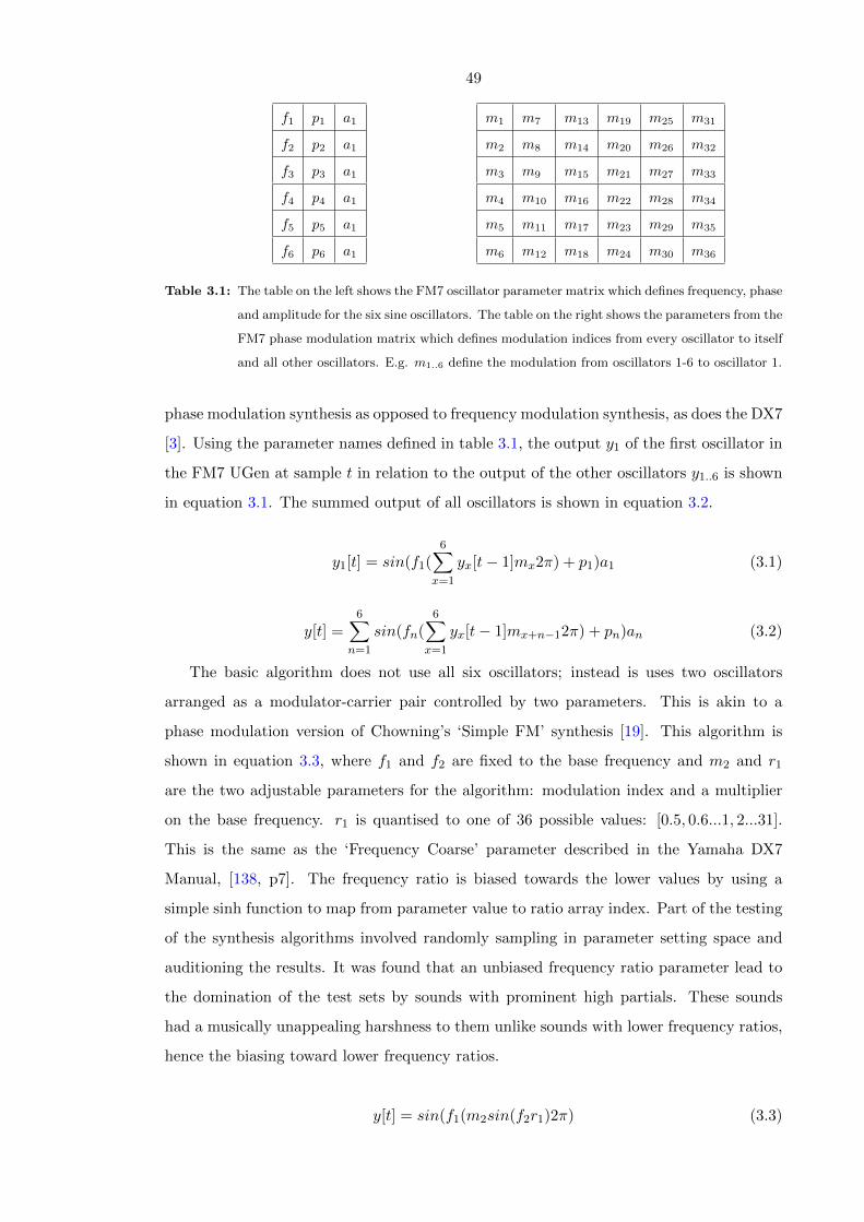
49

f1 p1 a1

f2 p2 a1

f3 p3 a1

f4 p4 a1

f5 p5 a1

f6 p6 a1

m1 m7 m13 m19 m25 m31

m2 m8 m14 m20 m26 m32

m3 m9 m15 m21 m27 m33

m4 m10 m16 m22 m28 m34

m5 m11 m17 m23 m29 m35

m6 m12 m18 m24 m30 m36

Table 3.1: The table on the left shows the FM7 oscillator parameter matrix which defines frequency, phase

and amplitude for the six sine oscillators. The table on the right shows the parameters from the

FM7 phase modulation matrix which defines modulation indices from every oscillator to itself

and all other oscillators. E.g. m1..6 define the modulation from oscillators 1-6 to oscillator 1.

phase modulation synthesis as opposed to frequency modulation synthesis, as does the DX7

[3]. Using the parameter names defined in table 3.1, the output y1 of the first oscillator in

the FM7 UGen at sample t in relation to the output of the other oscillators y1..6 is shown

in equation 3.1. The summed output of all oscillators is shown in equation 3.2.

y1[t] = sin(f1(6∑

x=1

yx[t− 1]mx2π) + p1)a1 (3.1)

y[t] =6∑

n=1

sin(fn(6∑

x=1

yx[t− 1]mx+n−12π) + pn)an (3.2)

The basic algorithm does not use all six oscillators; instead is uses two oscillators

arranged as a modulator-carrier pair controlled by two parameters. This is akin to a

phase modulation version of Chowning’s ‘Simple FM’ synthesis [19]. This algorithm is

shown in equation 3.3, where f1 and f2 are fixed to the base frequency and m2 and r1

are the two adjustable parameters for the algorithm: modulation index and a multiplier

on the base frequency. r1 is quantised to one of 36 possible values: [0.5, 0.6...1, 2...31].

This is the same as the ‘Frequency Coarse’ parameter described in the Yamaha DX7

Manual, [138, p7]. The frequency ratio is biased towards the lower values by using a

simple sinh function to map from parameter value to ratio array index. Part of the testing

of the synthesis algorithms involved randomly sampling in parameter setting space and

auditioning the results. It was found that an unbiased frequency ratio parameter lead to

the domination of the test sets by sounds with prominent high partials. These sounds

had a musically unappealing harshness to them unlike sounds with lower frequency ratios,

hence the biasing toward lower frequency ratios.

y[t] = sin(f1(m2sin(f2r1)2π) (3.3)

50

The complex algorithm uses three oscillators and is controlled by 22 parameters. Mod-

ulation from oscillator to oscillator is controlled by a single parameter per oscillator which

decides which of several available modulation routings from that oscillator to other oscilla-

tors are chosen. The available routings for each of the three oscillators are [0, 0, 0], [1, 0, 0],

[0, 1, 0], [1, 1, 0], [0, 0, 1], [1, 0, 1] and [0, 1, 1], or ‘no modulation’, ‘modulate oscillator one’,

‘modulate oscillator two’, ‘modulate oscillators one and two’, ‘modulate oscillator three’,

‘modulate oscillators one and three’ and ‘modulate oscillators two and three’, respectively.

This is similar to the feature found on the DX7 which allows the user to choose different

algorithms, [138, p24]. A further three parameters per oscillator define the modulation

indices to the three other oscillators, the m1,2,3,7,8,9,13,14,15 values from table 3.1. Finally,

the oscillators are tuned using another three parameters per oscillator: coarse tuning, fine

tuning and detune. Coarse tuning is the same as for the basic synthesizer, fine tuning

adds up to 1 to the coarse tuning ratio and is continuous, detuning adds or subtracts up

to 10% from the final scaled frequency and is continuous. For example, let us consider the

case where the coarse tuning parameter is set to 0.5, the fine tuning 0.25 and the detune

is 0.75. Within the synthesizer, the coarse ratio r1 will be 3 (the 8th element from the list

of 36, noting the biasing toward the lower end ratios); the fine ratio r2 will be 0.25; the

detune d will be +5%. Using equation 3.4 to calculate the resulting frequency f for this

oscillator with a base frequency F of 440Hz yields the result 1440.725Hz.

f = F (r1 + r2)(1 +d

100) (3.4)

A final parameter is used to choose from a set of available settings for switches which

will allow one or more oscillators to be routed to the audio out. For example, switch

settings of [1,0,1] would allow oscillators 1 and 3 to be heard. The parameters are further

described in table 3.2.

3.1.2 Subtractive Synthesis

The basic subtractive synthesis algorithm takes the three parameters listed in table 3.3.

The cut off and reciprocal of Q are standard filter parameters but the oscillator mix

parameter requires further explanation. The oscillator mix is the amount of each of the four

oscillators sent to the audio output, where the available oscillators generate sin, sawtooth,

pulse and white noise waveforms. In order to specify the mix using a single parameter,

the parameter is used to select from one of many sets of levels for the oscillators, The

available levels are restricted so that only two oscillators can be active at a time. For

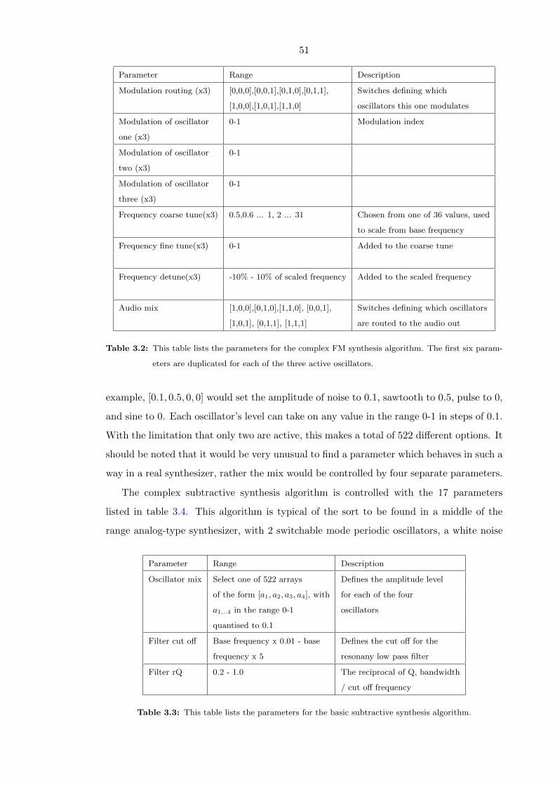
51

Parameter Range Description

Modulation routing (x3) [0,0,0],[0,0,1],[0,1,0],[0,1,1], Switches defining which

[1,0,0],[1,0,1],[1,1,0] oscillators this one modulates

Modulation of oscillator 0-1 Modulation index

one (x3)

Modulation of oscillator 0-1

two (x3)

Modulation of oscillator 0-1

three (x3)

Frequency coarse tune(x3) 0.5,0.6 ... 1, 2 ... 31 Chosen from one of 36 values, used

to scale from base frequency

Frequency fine tune(x3) 0-1 Added to the coarse tune

Frequency detune(x3) -10% - 10% of scaled frequency Added to the scaled frequency

Audio mix [1,0,0],[0,1,0],[1,1,0], [0,0,1], Switches defining which oscillators

[1,0,1], [0,1,1], [1,1,1] are routed to the audio out

Table 3.2: This table lists the parameters for the complex FM synthesis algorithm. The first six param-

eters are duplicated for each of the three active oscillators.

example, [0.1, 0.5, 0, 0] would set the amplitude of noise to 0.1, sawtooth to 0.5, pulse to 0,

and sine to 0. Each oscillator’s level can take on any value in the range 0-1 in steps of 0.1.

With the limitation that only two are active, this makes a total of 522 different options. It

should be noted that it would be very unusual to find a parameter which behaves in such a

way in a real synthesizer, rather the mix would be controlled by four separate parameters.

The complex subtractive synthesis algorithm is controlled with the 17 parameters

listed in table 3.4. This algorithm is typical of the sort to be found in a middle of the

range analog-type synthesizer, with 2 switchable mode periodic oscillators, a white noise

Parameter Range Description

Oscillator mix Select one of 522 arrays Defines the amplitude level

of the form [a1, a2, a3, a4], with for each of the four

a1...4 in the range 0-1 oscillators

quantised to 0.1

Filter cut off Base frequency x 0.01 - base Defines the cut off for the

frequency x 5 resonany low pass filter

Filter rQ 0.2 - 1.0 The reciprocal of Q, bandwidth

/ cut off frequency

Table 3.3: This table lists the parameters for the basic subtractive synthesis algorithm.

52

oscillator and 3 resonant filters.

3.1.3 Variable Architecture Synthesis

The variable architecture synthesizer was initially modelled after an old fashioned analog

modular synthesizer, where a variable number of parameterised modules are connected

together. However, it was found that the SuperCollider non real time synthesis engine

was not suitable for the attempted implementation as it was found to render certain

types of sounds inconsistently or not at all. In addition, a non-functional sound would

sometimes prevent all subsequent sounds in that batch from rendering correctly. Whilst

such a constraint could be viewed as simply another part of the challenge to the optimisers,

i.e. to find sounds that SuperCollider can render consistently as well as being close to the

target sounds, in practise it slowed down the optimisers to the point of being unusable

for the large test sets. This is not to say that the SuperCollider system cannot model a

modular synthesizer, but that the modular system designed for this work was not suitable

for SuperCollider. It is hoped that in future work, it will be possible to implement an

optimisable analog-style modular synthesizer.

The eventual variable architecture synthesizer was therefore made from a single type of

module, implementing frequency modulation synthesis using a single sine wave oscillator

per module. The synthesizer uses 6 buses to share modulation data between the modules

and for the purposes of this experiment has between 5 and 50 modules. The parameters

for the module are described in table 3.5. This synthesis architecture can generate a wide

range of sounds and provides a highly complex search space.

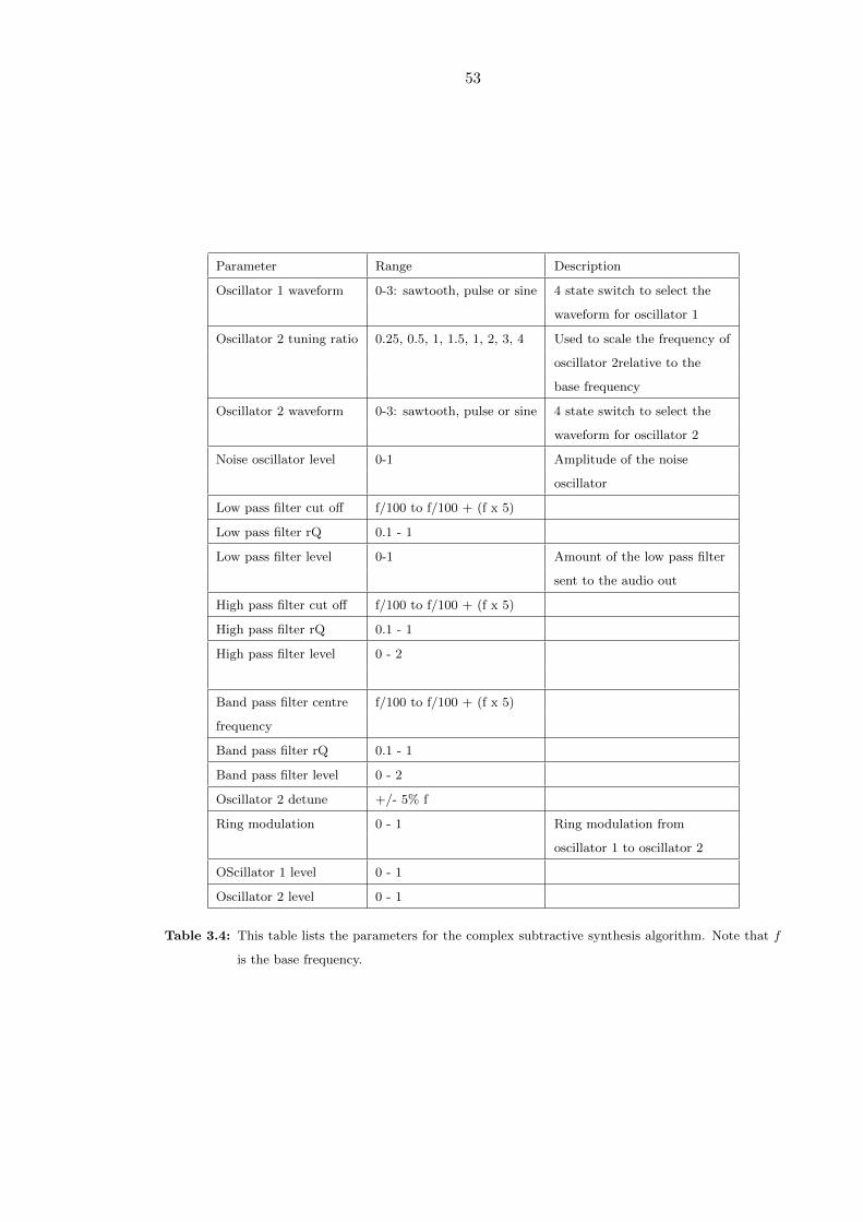
53

Parameter Range Description

Oscillator 1 waveform 0-3: sawtooth, pulse or sine 4 state switch to select the

waveform for oscillator 1

Oscillator 2 tuning ratio 0.25, 0.5, 1, 1.5, 1, 2, 3, 4 Used to scale the frequency of

oscillator 2relative to the

base frequency

Oscillator 2 waveform 0-3: sawtooth, pulse or sine 4 state switch to select the

waveform for oscillator 2

Noise oscillator level 0-1 Amplitude of the noise

oscillator

Low pass filter cut off f/100 to f/100 + (f x 5)

Low pass filter rQ 0.1 - 1

Low pass filter level 0-1 Amount of the low pass filter

sent to the audio out

High pass filter cut off f/100 to f/100 + (f x 5)

High pass filter rQ 0.1 - 1

High pass filter level 0 - 2

Band pass filter centre f/100 to f/100 + (f x 5)

frequency

Band pass filter rQ 0.1 - 1

Band pass filter level 0 - 2

Oscillator 2 detune +/- 5% f

Ring modulation 0 - 1 Ring modulation from

oscillator 1 to oscillator 2

OScillator 1 level 0 - 1

Oscillator 2 level 0 - 1

Table 3.4: This table lists the parameters for the complex subtractive synthesis algorithm. Note that f

is the base frequency.

54

Parameter Range Description

FM index 0-(f/5) Scales the modulation

FM input bus 32-37 FM is read from this bus

Frequency ratio one of 0.0625.0.125, Scales the base

0.25, 0.5, 1,2 ...6 frequency

Audio output 0-1 Scales the audible

level output of this module

FM output bus 32-37 Write output to this bus

Detune ratio -0.025-0.025 Added to the frequency

ratio

Table 3.5: This table shows the parameters for the variable architecture synthesis algorithm. f is the

base frequency.

3.2 Synthesis Feature Space Analysis

During the development and testing of the optimisation algorithms, it became obvious

that an analysis of the feature space of the synthesizers would be interesting and that

it might feed into the design of the optimisers. For example, the data driven nearest

neighbour algorithm (3.3.4) depends on a large data set sampled from feature space; but

how should this data set best be sampled? The neural networks depend on training sets

and test sets, but what should be in these sets? In the following subsection, the idea of an

error surface is introduced and the error surfaces of the various sound synthesis algorithms

are examined in detail.

3.2.1 Error Surface Analysis

The error surface is loosely defined here as the variation in the distance from a reference

point in feature space as one or more synthesis parameters are adjusted. In this case,

the distance metric is the square root of the sum squared Euclidean distance between the

reference vector t and the error surface ‘reading’ e (see equation 3.5). The error surface is

similar to the fitness landscape often discussed in genetic algorithm and evolution theory

research where the reference point would be taken as the target for the GA and the fitness

would be some inverse manipulation of the distance from this reference point [61, p33].

d =√

(42∑n=1

(t[n]− e[n])2) (3.5)

Euclidean distances and error surfaces are precise ways to compare sounds, but what

is the perceptual significance of an error of 1.5 vs an error of 2.7, for example? Since the

55

Instrument Dissimilarity Matrix: attack

Flute

Cello

Piano

Sax

Horn

Trumpet

Bassoon

Oboe

Violin

Clarinet

Flu

te

Cello

Pia

no

Sax

Horn

Tru

mpet

Bassoon

Oboe

Vio

lin

Cla

rinet

0

1

2

3

4

5

Instrument Dissimilarity Matrix: sustain

Flute

Cello

Piano

Sax

Horn

Trumpet

Bassoon

Oboe

Violin

Clarinet

Flu

te

Cello

Pia

no

Sax

Horn

Tru

mpet

Bassoon

Oboe

Vio

lin

Cla

rinet

0

1

2

3

4

5

Figure 3.1: This image shows the distances in MFCC feature space between the ten instrument samples

used as targets for the optimisers. The higher the value, the greater the distance and therefore

the dissimilarity. The left matrix compares the attack portions of the instruments, the right

compares the sustain periods, defined as the first 25 feature vectors and feature vectors 50-75,

respectively.

difference between a cello and a French horn is most likely more familiar to the reader

than the difference between a mathematically described FM synthesis algorithm with a

modulation index of 0.5 or 1.5, that question can be loosely answered by considering the

error between the different instruments used in the optimisation task that is the main focus

of this chapter. Figure 3.1 shows distance matrices between the ten instruments used to

test the optimisers. (The instrument samples were taken from [37]). The value being

plotted is the error in MFCC feature space between the different instruments. This value

is calculated by taking the 42 dimensional mean of 25 consecutive MFCC feature vectors

starting at frame 0 and frame 50 into the sound, for the attack and sustain plots, and

generating the error from the other instruments using equation 3.5. Since the instruments

are sampled at 44100Hz and the hop size on the feature vector is 512 frames, the time being

considered here is about 0.3s. Comparing the error observed between instruments to figure

3.3 which shows the error observed when a synthesis parameter is varied, it is possible to

say that a variation from 0.5 to 0.45 in parameter space causes that synthesizer’s output

sound to change as much as the difference between the steady state portions of an oboe

and a trumpet.

In the following subsections, the error surfaces of the different synthesizers are exam-

ined, firstly to establish the resolution required to represent them accurately and then to

describe the variation of the terrain observed as parameters are changed.

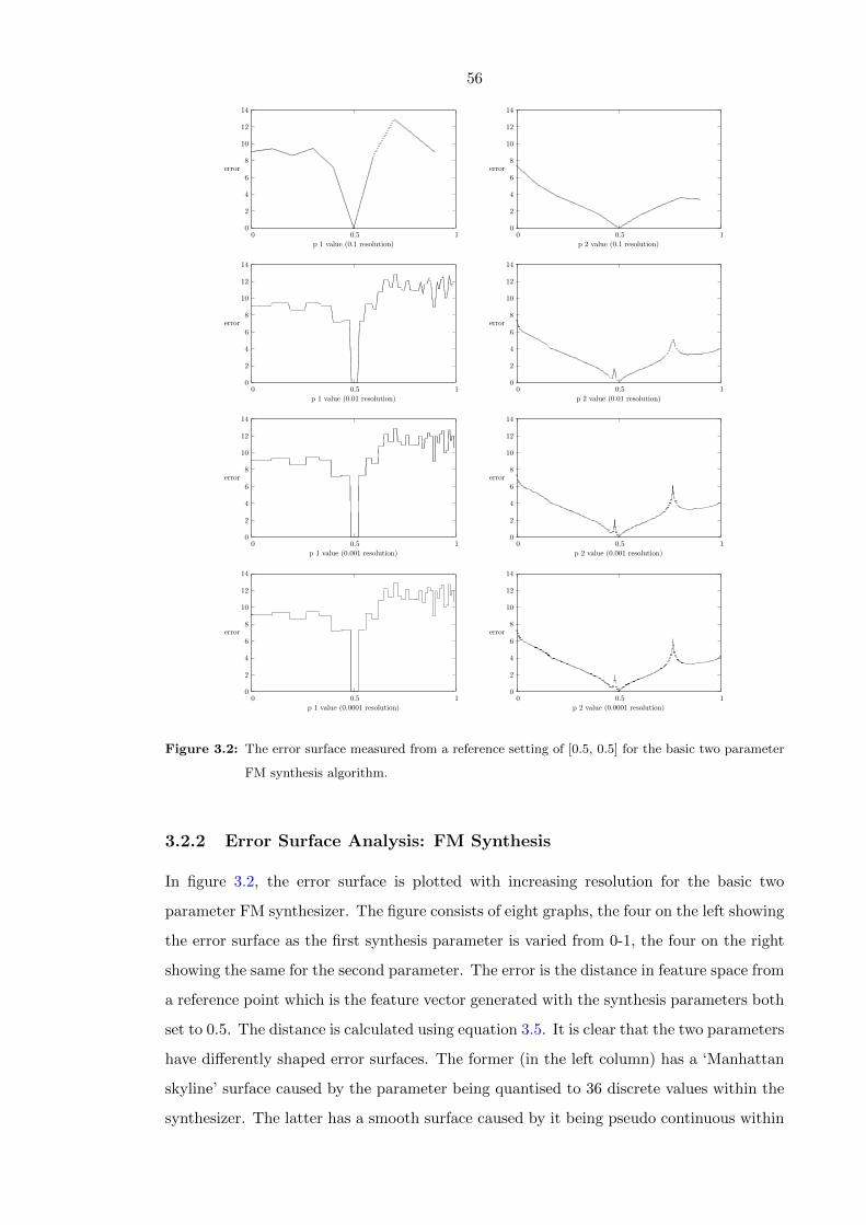
56

0

2

4

6

8

10

12

14

0 0.5 1

error

p 1 value (0.1 resolution)

0

2

4

6

8

10

12

14

0 0.5 1

error

p 2 value (0.1 resolution)

0

2

4

6

8

10

12

14

0 0.5 1

error

p 1 value (0.01 resolution)

0

2

4

6

8

10

12

14

0 0.5 1

error

p 2 value (0.01 resolution)

0

2

4

6

8

10

12

14

0 0.5 1

error

p 1 value (0.001 resolution)

0

2

4

6

8

10

12

14

0 0.5 1

error

p 2 value (0.001 resolution)

0

2

4

6

8

10

12

14

0 0.5 1

error

p 1 value (0.0001 resolution)

0

2

4

6

8

10

12

14

0 0.5 1

error

p 2 value (0.0001 resolution)

Figure 3.2: The error surface measured from a reference setting of [0.5, 0.5] for the basic two parameter

FM synthesis algorithm.

3.2.2 Error Surface Analysis: FM Synthesis

In figure 3.2, the error surface is plotted with increasing resolution for the basic two

parameter FM synthesizer. The figure consists of eight graphs, the four on the left showing

the error surface as the first synthesis parameter is varied from 0-1, the four on the right

showing the same for the second parameter. The error is the distance in feature space from

a reference point which is the feature vector generated with the synthesis parameters both

set to 0.5. The distance is calculated using equation 3.5. It is clear that the two parameters

have differently shaped error surfaces. The former (in the left column) has a ‘Manhattan

skyline’ surface caused by the parameter being quantised to 36 discrete values within the

synthesizer. The latter has a smooth surface caused by it being pseudo continuous within

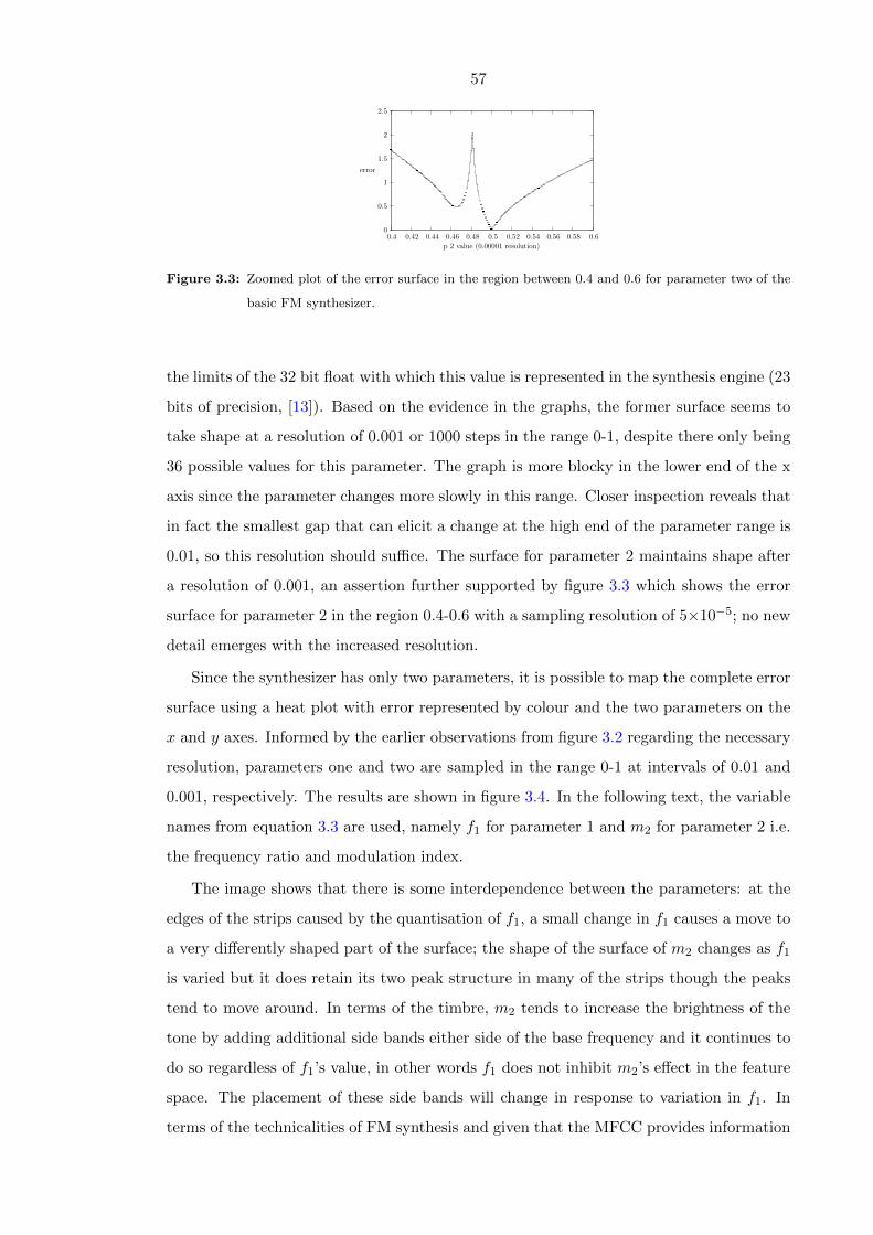
57

0

0.5

1

1.5

2

2.5

0.4 0.42 0.44 0.46 0.48 0.5 0.52 0.54 0.56 0.58 0.6

error

p 2 value (0.00001 resolution)

Figure 3.3: Zoomed plot of the error surface in the region between 0.4 and 0.6 for parameter two of the

basic FM synthesizer.

the limits of the 32 bit float with which this value is represented in the synthesis engine (23

bits of precision, [13]). Based on the evidence in the graphs, the former surface seems to

take shape at a resolution of 0.001 or 1000 steps in the range 0-1, despite there only being

36 possible values for this parameter. The graph is more blocky in the lower end of the x

axis since the parameter changes more slowly in this range. Closer inspection reveals that

in fact the smallest gap that can elicit a change at the high end of the parameter range is

0.01, so this resolution should suffice. The surface for parameter 2 maintains shape after

a resolution of 0.001, an assertion further supported by figure 3.3 which shows the error

surface for parameter 2 in the region 0.4-0.6 with a sampling resolution of 5×10−5; no new

detail emerges with the increased resolution.

Since the synthesizer has only two parameters, it is possible to map the complete error

surface using a heat plot with error represented by colour and the two parameters on the

x and y axes. Informed by the earlier observations from figure 3.2 regarding the necessary

resolution, parameters one and two are sampled in the range 0-1 at intervals of 0.01 and

0.001, respectively. The results are shown in figure 3.4. In the following text, the variable

names from equation 3.3 are used, namely f1 for parameter 1 and m2 for parameter 2 i.e.

the frequency ratio and modulation index.

The image shows that there is some interdependence between the parameters: at the

edges of the strips caused by the quantisation of f1, a small change in f1 causes a move to

a very differently shaped part of the surface; the shape of the surface of m2 changes as f1

is varied but it does retain its two peak structure in many of the strips though the peaks

tend to move around. In terms of the timbre, m2 tends to increase the brightness of the

tone by adding additional side bands either side of the base frequency and it continues to

do so regardless of f1’s value, in other words f1 does not inhibit m2’s effect in the feature

space. The placement of these side bands will change in response to variation in f1. In

terms of the technicalities of FM synthesis and given that the MFCC provides information

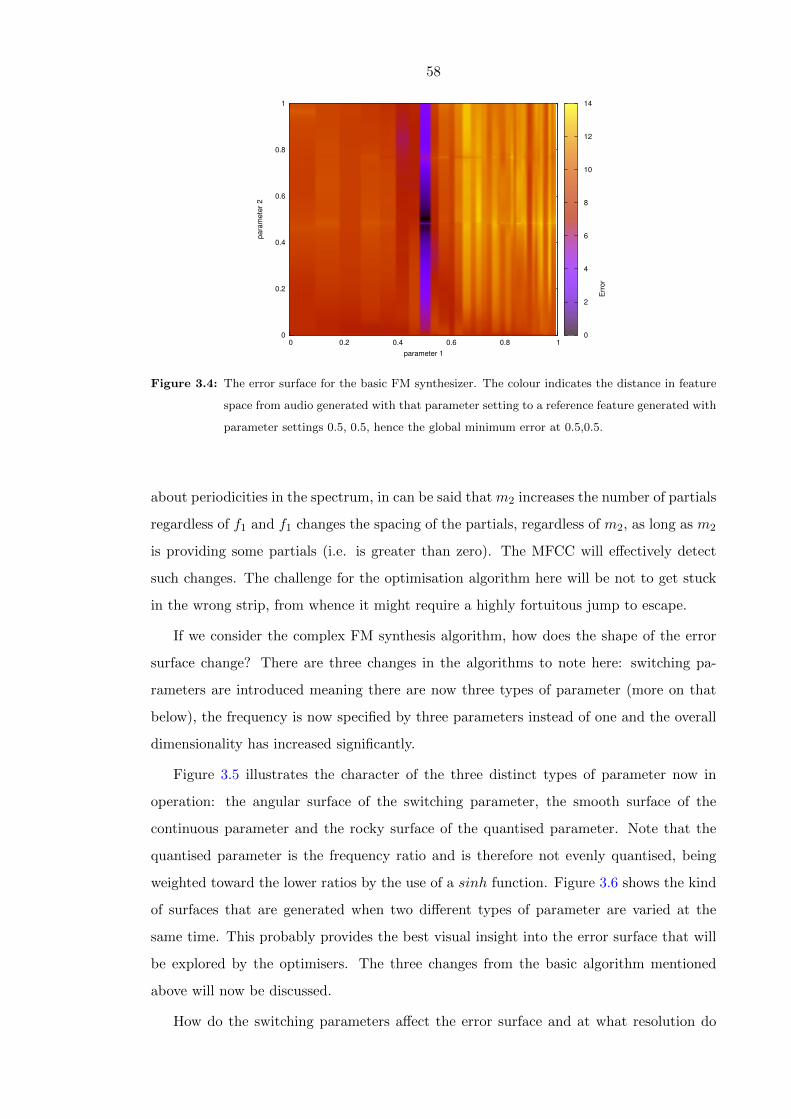
58

0

0.2

0.4

0.6

0.8

1

0 0.2 0.4 0.6 0.8 1

para

mete

r 2

parameter 1

Err

or

’../BasicFMOS_p0_at_0.01_vs_p1_at_0.001_ref_0.5.txt’

0

2

4

6

8

10

12

14

Figure 3.4: The error surface for the basic FM synthesizer. The colour indicates the distance in feature

space from audio generated with that parameter setting to a reference feature generated with

parameter settings 0.5, 0.5, hence the global minimum error at 0.5,0.5.

about periodicities in the spectrum, in can be said that m2 increases the number of partials

regardless of f1 and f1 changes the spacing of the partials, regardless of m2, as long as m2

is providing some partials (i.e. is greater than zero). The MFCC will effectively detect

such changes. The challenge for the optimisation algorithm here will be not to get stuck

in the wrong strip, from whence it might require a highly fortuitous jump to escape.

If we consider the complex FM synthesis algorithm, how does the shape of the error

surface change? There are three changes in the algorithms to note here: switching pa-

rameters are introduced meaning there are now three types of parameter (more on that

below), the frequency is now specified by three parameters instead of one and the overall

dimensionality has increased significantly.

Figure 3.5 illustrates the character of the three distinct types of parameter now in

operation: the angular surface of the switching parameter, the smooth surface of the

continuous parameter and the rocky surface of the quantised parameter. Note that the

quantised parameter is the frequency ratio and is therefore not evenly quantised, being

weighted toward the lower ratios by the use of a sinh function. Figure 3.6 shows the kind

of surfaces that are generated when two different types of parameter are varied at the

same time. This probably provides the best visual insight into the error surface that will

be explored by the optimisers. The three changes from the basic algorithm mentioned

above will now be discussed.

How do the switching parameters affect the error surface and at what resolution do

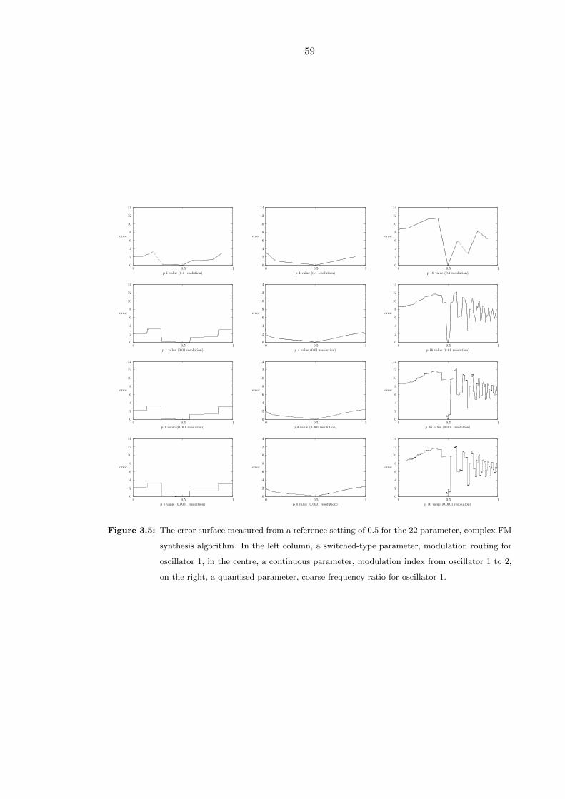
59

0

2

4

6

8

10

12

14

0 0.5 1

error

p 1 value (0.1 resolution)

0

2

4

6

8

10

12

14

0 0.5 1

error

p 4 value (0.1 resolution)

0

2

4

6

8

10

12

14

0 0.5 1

error

p 16 value (0.1 resolution)

0

2

4

6

8

10

12

14

0 0.5 1

error

p 1 value (0.01 resolution)

0

2

4

6

8

10

12

14

0 0.5 1

error

p 4 value (0.01 resolution)

0

2

4

6

8

10

12

14

0 0.5 1

error

p 16 value (0.01 resolution)

0

2

4

6

8

10

12

14

0 0.5 1

error

p 1 value (0.001 resolution)

0

2

4

6

8

10

12

14

0 0.5 1

error

p 4 value (0.001 resolution)

0

2

4

6

8

10

12

14

0 0.5 1

error

p 16 value (0.001 resolution)

0

2

4

6

8

10

12

14

0 0.5 1

error

p 1 value (0.0001 resolution)

0

2

4

6

8

10

12

14

0 0.5 1

error

p 4 value (0.0001 resolution)

0

2

4

6

8

10

12

14

0 0.5 1

error

p 16 value (0.0001 resolution)

Figure 3.5: The error surface measured from a reference setting of 0.5 for the 22 parameter, complex FM

synthesis algorithm. In the left column, a switched-type parameter, modulation routing for

oscillator 1; in the centre, a continuous parameter, modulation index from oscillator 1 to 2;

on the right, a quantised parameter, coarse frequency ratio for oscillator 1.

60

0

0.2

0.4

0.6

0.8

1

0 0.2 0.4 0.6 0.8 1

para

mete

r 16

parameter 1

Err

or

’../InterFMOS_p0_at_0.05_vs_p15_at_0.002_ref_0.5.txt’

0

2

4

6

8

10

12

14

0

0.2

0.4

0.6

0.8

1

0 0.2 0.4 0.6 0.8 1

para

mete

r 5

parameter 1

Err

or

’../InterFMOS_p0_at_0.05_vs_p4_at_0.002_ref_0.5.txt’

0

2

4

6

8

10

12

14

0

0.2

0.4

0.6

0.8

1

0 0.2 0.4 0.6 0.8 1

para

mete

r 16

parameter 5

Err

or

’../InterFMOS_p4_at_0.005_vs_p15_at_0.005_ref_0.5.txt’

0

2

4

6

8

10

12

14

Figure 3.6: Two-parameter error surfaces for the complex FM synthesizer: modulation routing vs fre-

quency ratio, modulation routing vs modulation index, modulation index vs modulation

routing.

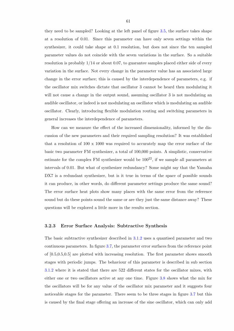
61

they need to be sampled? Looking at the left panel of figure 3.5, the surface takes shape

at a resolution of 0.01. Since this parameter can have only seven settings within the

synthesizer, it could take shape at 0.1 resolution, but does not since the ten sampled

parameter values do not coincide with the seven variations in the surface. So a suitable

resolution is probably 1/14 or about 0.07, to guarantee samples placed either side of every

variation in the surface. Not every change in the parameter value has an associated large

change in the error surface; this is caused by the interdependence of parameters, e.g. if

the oscillator mix switches dictate that oscillator 3 cannot be heard then modulating it

will not cause a change in the output sound, assuming oscillator 3 is not modulating an

audible oscillator, or indeed is not modulating an oscillator which is modulating an audible

oscillator. Clearly, introducing flexible modulation routing and switching parameters in

general increases the interdependence of parameters.

How can we measure the effect of the increased dimensionality, informed by the dis-

cussion of the new parameters and their required sampling resolution? It was established

that a resolution of 100 x 1000 was required to accurately map the error surface of the

basic two parameter FM synthesizer, a total of 100,000 points. A simplistic, conservative

estimate for the complex FM synthesizer would be 10022, if we sample all parameters at

intervals of 0.01. But what of synthesizer redundancy? Some might say that the Yamaha

DX7 is a redundant synthesizer, but is it true in terms of the space of possible sounds

it can produce, in other words, do different parameter settings produce the same sound?

The error surface heat plots show many places with the same error from the reference

sound but do these points sound the same or are they just the same distance away? These

questions will be explored a little more in the results section.

3.2.3 Error Surface Analysis: Subtractive Synthesis

The basic subtractive synthesizer described in 3.1.2 uses a quantised parameter and two

continuous parameters. In figure 3.7, the parameter error surfaces from the reference point

of [0.5,0.5,0.5] are plotted with increasing resolution. The first parameter shows smooth

stages with periodic jumps. The behaviour of this parameter is described in sub section

3.1.2 where it is stated that there are 522 different states for the oscillator mixes, with

either one or two oscillators active at any one time. Figure 3.8 shows what the mix for

the oscillators will be for any value of the oscillator mix parameter and it suggests four

noticeable stages for the parameter. There seem to be three stages in figure 3.7 but this

is caused by the final stage offering an increase of the sine oscillator, which can only add

62

0

2

4

0 0.5 1

error

p 1 value (0.1 resolution)

0

2

4

0 0.5 1

error

p 2 value (0.1 resolution)

0

2

4

0 0.5 1

error

p 3 value (0.1 resolution)

0

2

4

0 0.5 1

error

p 1 value (0.01 resolution)

0

2

4

0 0.5 1

error

p 2 value (0.01 resolution)

0

2

4

0 0.5 1

error

p 3 value (0.01 resolution)

0

2

4

0 0.5 1

error

p 1 value (0.001 resolution)

0

2

4

0 0.5 1

error

p 2 value (0.001 resolution)

0

2

4

0 0.5 1

error

p 3 value (0.001 resolution)

0

2

4

0 0.5 1

error

p 1 value (0.0001 resolution)

0

2

4

0 0.5 1

error

p 2 value (0.0001 resolution)

0

2

4

0 0.5 1

error

p 3 value (0.0001 resolution)

Figure 3.7: The error surface measured from a reference setting of [0.5, 0.5, 0.5] for the basic three

parameter subtractive synthesis algorithm.

0 0.1 0.2 0.3 0.4 0.5 0.6 0.7 0.8 0.9 1

Oscillator mix parameter value

Oscillator Levels

noisesaw

pulsesin

Figure 3.8: The mix levels of each oscillator in the basic subtractive synthesizer as the oscillator mix

parameter is varied. Each oscillator can take on one of 10 mix levels.

63

a single partial to the sound, which does not appear to register in the error. Since this

parameter can take on 522 distinct states within the synthesizers, a resolution of 0.002

should be sufficient to map this parameter’s range of features. The continuous parameters

seem to require a fairly low resolution, taking shape at a resolution of 0.01.

Figure 3.9 contains heat plots showing how the three possible combinations of param-

eters affect each other. The quantised mix parameter only seems to have a large effect

from strip to strip, not within strips. This is because within a strip the oscillators are

being faded up, gradually varying the sound whereas between strips, the combination of

two oscillators is changed abruptly. It is anticipated that it will be challenging for simpler

optimisation algorithms to traverse these strips to find a global minimum, depending on

the hop size (in parameter space) of the optimiser, i.e. if the hop size is too low, the

optimiser is unlikely to escape a strip. The continuous parameters, i.e. the filter cut off

and rQ, show a smooth error surface which should be fairly trivial to search due to its

large, single valley of low error. If an optimiser finds itself stuck in a strip a long way

off from the target, it will be necessary to traverse several high error strips to reach the

target.

The error surface of the complex subtractive synthesizer is expected to be similar to

that for the basic synthesizer. The filter parameters behave in the same way and there

are switchable mode oscillators. The difference is that the oscillator volume controls have

been changed from a single quantised parameter to several continuous parameters.

The error surface for the variable architecture synthesizer is difficult to plot since it is

not clear what should be used as a reference point and what should be varied to create the

surface. It can be said that the parameters within a single module will behave similarly to

their equivalents in the basic and complex FM synthesizers but that a growth operation

which adds a module could cause a large movement in feature space as the new module

might modulate the existing modules as well as sending its signal to the audio out.

64

0

0.2

0.4

0.6

0.8

1

0 0.2 0.4 0.6 0.8 1

para

mete

r 2

parameter 1

Err

or

’..//BasicSubOS_p0_at_0.002_vs_p1_at_0.01_ref_0.5.txt’

0

1

2

3

4

5

6

0

0.2

0.4

0.6

0.8

1

0 0.2 0.4 0.6 0.8 1

para

mete

r 2

parameter 1

Err

or

’..//BasicSubOS_p0_at_0.002_vs_p2_at_0.01_ref_0.5.txt’

0

0.5

1

1.5

2

2.5

3

3.5

4

4.5

5

0

0.2

0.4

0.6

0.8

1

0 0.2 0.4 0.6 0.8 1

para

mete

r 2

parameter 1

Err

or

’..//BasicSubOS_p1_at_0.01_vs_p2_at_0.01_ref_0.5.txt’

0

0.5

1

1.5

2

2.5

3

3.5

4

4.5

Figure 3.9: Two-parameter error surfaces for the basic subtractive synthesizer: oscillator mix vs cut off,

oscillator mix vs rQ, and cut off vs rQ

65

3.3 The Optimisation Techniques

The optimisation problem is: ‘The elucidation of appropriate parameter settings for each

sound synthesis algorithm to enable resynthesis of 50 sounds generated by each synthe-

sis algorithm and of 10 real instrument samples, respectively.’. These two test sets are

chosen to enable maximum flexibility when comparing different optimisers and different

synthesizers. The first set consists of 50 pairs of randomly generated parameter settings

and resultant single frame feature vectors, per synthesizer. Since the test set is generated

with the same synthesizer that the optimiser is working with in each case, it is possible

to gain an error of zero, given a perfect optimiser. This test set enables the comparison

of different optimisers and different optimiser settings for a given synthesizer. The second

test set consists of two feature vector frames per instrument for the following instruments:

Alto Flute, Alto Sax, Bassoon, B[ Clarinet, Cello, French Horn, Oboe, Piano, Trumpet

and Violin. The selection of instruments was chosen based on its coverage of a range of

different sound production methods and its successful use in previous research, e.g.: [34]

used the same selection, [43] used eight of the ten, having found that musically trained

subjects found the sounds highly recognisable. The instrument samples were obtained

from the University of Iowa Electronic Music Studio collection [37]. All instruments were

playing vibrato-free C4 (middle C). The first frame is the 42 dimensional mean of 25

frames taken from the attack portion at the beginning of the sound; the second frame is

the 42 dimensional mean of 25 frames taken from approx 0.5s into the sound. It is unlikely

that a synthesizer will be able to perfectly replicate these sounds so the optimiser must

find the closest sound available. Since the synthesizers do not include envelope generators

to vary their sonic output over time, the optimiser must find the synthesis parameter

settings to generate each feature vector frame in turn. This test enables the comparison

of different synthesizers in their ability to resynthesize the samples. To summarise, each

of the 4 optimisers must find optimal parameter settings for 70 sounds for each of the 5

synthesizers, 50 that the synthesizer can match perfectly and 20 that it can probably only

approximate. This is a theoretical total of 1400 tests but only two of the optimisers are

appropriate for the variable architecture synthesizer, making the total 1260.

The optimisation techniques will now be described in detail.

3.3.1 Basic Hill Climbing

An introduction to hill climbing can be found in [69]. The hill climbing algorithm here is

implemented as follows:

66

Starting from a random population of 1000 sets of parameter settings, the output of

each set is rendered and features are extracted. The error between the target feature

and each of the 1000 candidate feature vectors is calculated using the Euclidean distance.

(equation 3.5). The score for each is calculated using equation 3.6. The candidate with

the highest score is used to seed the next population, which consists of mutated versions of

the seed. Mutating involves the addition of a value drawn from a uniform distribution in

the range -0.05 to +0.05 to a single parameter setting. A growth operation is also applied

if the candidate sound is to be generated with more than one module (e.g. the variable

architecture FM synthesizer.). The population is considered to have converged when the

mean change in top score over 20 generations is less than 0.01%.

3.3.2 Feed Forward Neural Network

A feed forward neural network is trained using a set of parameter settings and their

resultant feature vectors such that the network learns the mapping from feature vector

input to parameter setting output. Once trained, the network can be used to elicit the

parameter settings required to produce a given, previously unseen feature vector with a

particular synthesis algorithm. The implementation and elucidation of optimal properties

for the feed forward neural network is described in the following paragraphs.

A training set of data consisting of synthesis parameter settings and the resultant

feature vectors is created. The set consists of parameters and resultant features derived

by sampling parameter space randomly. A feed forward neural net with a single hidden

layer, based on code written by Collins and Kiefer [26], is created. The network has v

input nodes and p output nodes, where v is the size of the feature vector and p the number

of parameters provided by the synthesis algorithm. The network is trained using the back

propagation algorithm. There are several properties associated with this neural network

and the training procedure for which reasonable values must first be heuristically obtained.

They are learning rate, number of training epochs, number of hidden nodes and size of

the training set. These properties must be obtained for each synthesis method since the

number of parameters and the mapping varies significantly between them. The procedures

and results are summarised in figure 3.10 and discussed in the following subsections.

Learning Rate

The learning rate parameter determines the amount by which the neural network’s weights

are changed at each iteration of the back propagation algorithm. To establish the optimal

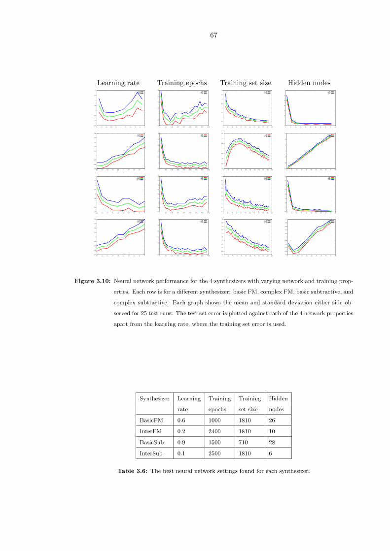
67

Learning rate Training epochs Training set size Hidden nodes

0.85

0.9

0.95

1

1.05

1.1

1.15

1.2

0 0.2 0.4 0.6 0.8 1 1.2 1.4 1.6 1.8 2

-1 sd

mean

+1 sd

0.8

0.9

1

1.1

1.2

1.3

1.4

0 500 1000 1500 2000 2500 3000 3500 4000

-1 sd

mean

+1 sd

0

0.5

1

1.5

2

2.5

3

3.5

4

0 20 40 60 80 100 120 140 160 180 200 220

-1 sd

mean

+1 sd

0

1

2

3

4

5

6

7

0 5 10 15 20 25 30 35 40 45 50

-1 sd

mean

+1 sd

0.97

0.98

0.99

1

1.01

1.02

1.03

1.04

1.05

0.1 0.2 0.3 0.4 0.5 0.6 0.7 0.8 0.9 1

-1 sd

mean

+1 sd

0.8

1

1.2

1.4

1.6

1.8

2

0 500 1000 1500 2000 2500 3000 3500 4000

-1 sd

mean

+1 sd

0.8

0.85

0.9

0.95

1

1.05

1.1

1.15

0 20 40 60 80 100 120 140 160 180 200 220

-1 sd

mean

+1 sd

0.7

0.8

0.9

1

1.1

1.2

1.3

0 5 10 15 20 25 30 35 40 45 50

-1 sd

mean

+1 sd

0.9

0.95

1

1.05

1.1

1.15

1.2

1.25

1.3

0.1 0.2 0.3 0.4 0.5 0.6 0.7 0.8 0.9 1

-1 sd

mean

+1 sd

0.8

0.9

1

1.1

1.2

1.3

1.4

1.5

1.6

0 500 1000 1500 2000 2500 3000 3500 4000

-1 sd

mean

+1 sd

0.6

0.8

1

1.2

1.4

1.6

1.8

2

2.2

2.4

0 20 40 60 80 100 120 140 160 180 200 220

-1 sd

mean

+1 sd

0.8

1

1.2

1.4

1.6

1.8

2

2.2

2.4

0 5 10 15 20 25 30 35 40 45 50

-1 sd

mean

+1 sd

0.96

0.97

0.98

0.99

1

1.01

1.02

1.03

1.04

0.1 0.2 0.3 0.4 0.5 0.6 0.7 0.8 0.9 1

-1 sd

mean

+1 sd

0.8

1

1.2

1.4

1.6

1.8

2

0 500 1000 1500 2000 2500 3000 3500 4000

-1 sd

mean

+1 sd

0.8

0.85

0.9

0.95

1

1.05

1.1

1.15

1.2

1.25

1.3

0 20 40 60 80 100 120 140 160 180 200 220

-1 sd

mean

+1 sd

0.9

0.92

0.94

0.96

0.98

1

1.02

1.04

1.06

1.08

1.1

0 5 10 15 20 25 30 35 40 45 50

-1 sd

mean

+1 sd

Figure 3.10: Neural network performance for the 4 synthesizers with varying network and training prop-

erties. Each row is for a different synthesizer: basic FM, complex FM, basic subtractive, and

complex subtractive. Each graph shows the mean and standard deviation either side ob-

served for 25 test runs. The test set error is plotted against each of the 4 network properties

apart from the learning rate, where the training set error is used.

Synthesizer Learning Training Training Hidden

rate epochs set size nodes

BasicFM 0.6 1000 1810 26

InterFM 0.2 2400 1810 10

BasicSub 0.9 1500 710 28

InterSub 0.1 2500 1810 6

Table 3.6: The best neural network settings found for each synthesizer.

68

learning rate, the network is trained with varying learning rates and the training set error

is calculated. This test is repeated 25 times with different, random training sets. The

learning rate which provides a good combination of low error over the training set and

lack of oscillation is selected. Oscillation is where the network learns some training sets

well and others not very well. In figure 3.10 column one, the results of this test for the

four synthesizers are shown. The values chosen for the synthesizers are shown in table 3.6

Training Epochs

The training epochs parameter is the number of iterations of training that are carried

out. To establish the appropriate number of training epochs, the test set error is graphed

against the number of training epochs. 25 runs are carried out for varying numbers of

epochs, each run with a different, random training set and test set. The expectation is

that the error will level out when sufficient epochs have been used. The results are graphed

in figure 3.10 and tabulated in 3.6. The error is seen to reduce to its lowest point then

to increase as over-fitting to the training set increases and generalisation to the test sets

decreases.

Hidden Nodes

The neural network has a single, fully connected hidden layer and this property defines

the number of nodes in that layer. In order to establish the optimal number of hidden

nodes, the test set error is measured against the number of hidden nodes. The expectation

is that the error will cease to decrease with increased node count when there are enough

nodes. The network is trained and tested with increasing numbers of hidden nodes. This

test is repeated 25 times with random test and training sets. The results are graphed in

figure 3.10 and tabulated in 3.6. The basic synthesizers behave as expected here, showing

a test error which levels once sufficient hidden nodes are in use. The complex synthesizers

show a more puzzling result, where the optimal number of hidden nodes seems to be very

low, considering the complexity of the synthesizer and therefore of the parameter setting

to feature mapping. The error also increases significantly with increasing numbers of

hidden nodes. In order to establish if the error would level out and maybe decrease with

increasing numbers of hidden nodes, extended tests were carried out with node counts

up to 1500 with these two synthesizers. The results are shown in figure 3.11. The error

levels out after around 600 nodes but shows no signs of decreasing. Since the mapping

for the simple synthesizers is learned with more nodes than 10 and that this low number

69

3200

3400

3600

3800

4000

4200

4400

4600

4800

5000

0 200 400 600 800 1000 1200 1400 1600

test set error

no. hidden nodes

Figure 3.11: This graph shows the results of increasing the number of hidden nodes for the complex FM

synthesizer to an unusually high level.

of nodes is therefore not sufficient to model the mapping for a more complex synthesizer,

this implies that this network architecture is not capable of modelling the mappings for

the complex FM and subtractive synthesizers. More on this in the results section.

Training Set Size

To establish the optimal training set size, the error over a large test set is calculated with

increasing training set size. This test is repeated 25 times with random test and training

sets. Once the error over the test set is seen to level out, the training set size is judged

as sufficient as increasing the size does not decrease the test set error. The results are

graphed in figure 3.10 and tabulated in 3.6.

3.3.3 Genetic Algorithm

The genetic algorithm used in this test is a standard model with the following features:

Single Population

The genomes exist in a single population and can be bred freely.

Genetic Operators

The genomes can undergo point mutation and crossover using two parents and variable

numbers of crossover points. The point mutation is controlled by two parameters, one

for the per-locus probability of mutation (mutation rate), the other for the size range of

the mutation (mutation size). Once a locus is chosen for mutation, the mutation size is

chosen from a Gaussian distribution with the mean set to zero and the standard deviation

set to the value of this second mutation parameter. The mutation rate is set to 1/(synth

parameter count), so at least one parameter is mutated per genome, on average. The

mutation size is set to 0.1.

70

Elitism

The best genome each iteration is kept.

Roulette Wheel Selection

When generating a new population, each new genome is created from two parent genomes.

The parent genomes are selected with a probability that is proportional to their fitness

relative to the population mean. This is roulette wheel selection. Every member of the

population is on the roulette wheel but the fitter they are, they more ‘slots’ they take

up and thus the more probable it is that they will be chosen. Roulette wheel selection

maintains diversity in the population by preventing the fittest individuals from taking

over in the case where their fitness is only marginally higher than other members of the

population. Maintaining diversity is especially useful when it comes to avoiding getting

stuck on local maxima. Let us consider the error surface plot shown in 3.4. Maintaining

a diverse population makes it possible to search different parts of the error surface in

parallel. This is the multi plane sampling discussed by Whitley [131]. It is possible to

further investigate the different properties of the GA and this has been done to a certain

extent in the other chapters. For example, in [131] Whitley recommends use of rank based

selection of breeding pairs as opposed to fitness proportional selection since it maintains

the selective pressure when the population begins to converge. The motivation for the

investigation of these finer points of GA implementation in order to produce a more

refined, optimised version should be taken from evidence of poor performance of the basic

implementation. The preliminary results indicated decent performance for the GA so it

was left in its basic state.

General Settings

For the tests, the algorithm was run with a population size of 1000 and a maximum of 500

iterations. The mutation rate was set to 1/(number of synthesis parameters) such that

there would on average be a single point mutation per genome. The mutation size range

was set to 0.1, i.e. the centre of the Gaussian distribution was placed at 0.1.

3.3.4 Basic Data Driven ‘Nearest Neighbour’ Approach

In this approach, the space of possible parameter settings is randomly sampled to produce

a data set of parameter settings and resultant feature vectors. Upon being presented

with a target feature vector, the system finds the feature vector in the data set which is

71

the closest to the target and can then provide the associated synthesis parameters. For

effective performance, this system is dependent on the ability to store and search a high

resolution data set which covers the full timbral range of the synthesizer. The parameters

for this optimiser are the data set size and the distance measure. Let us consider the

construction of the data set in more detail.

The data set must be sampled at sufficient resolution such that the detail of feature

vector space is high enough to represent the timbral range of the synthesizer. Consider

3.2 which shows the error in feature space from a reference setting of 0.5 as a single

parameter is varied from 0 to 1 with different levels of resolution. Once the resolution

reaches a sufficient level, the graph does not change with further increases: the true shape

of the error surface has been ascertained. In the case of the basic FM synthesis algorithm

shown in figure 3.2, the graph stops changing at around the 0.005 point, meaning it is

necessary to sample this synthesizer at steps of 0.005 for this particular parameter. In

the SuperCollider system, the parameters are stored as 32 bit floats, which offer some

23 bits of precision, providing usable resolution in the 1223

range; sampling at intervals of

0.005 is well within these limits. For a synthesizer with two parameters, assuming equal

sampling resolution for each, a data set of 40,000 items will be generated ((1/0.005)2).

If we consider the complex FM algorithm, it might initially seem that an impracticably

large data set of (1/0.005)19 or 5.24288e+43 items is required but this does not take into

account the quantised parameters or the redundancy of the synthesizer, where different

parameter settings generate the same sound.

3.4 Results

In this section, the results of applying the optimisation techniques to the problem defined

at the start of section 3.3 will be presented. The scope of the test is quite broad, so

the results are presented in summary. There are two main values used to quantify the

performance results in this section: the score and the error. The score is the reciprocal

of the normalised, sum, squared and rooted Euclidean distance from the target to the

candidate feature vector, as shown in equation 3.6. The figure of 42 used to normalise

the value is the size of the MFCC feature vector. The other value, the error, is simply

the sum, squared and rooted Euclidean distance betwixt target and candidate. The error

value is comparable with the values plotted in the graphs and heat plots from the error

surface analysis in subsection 3.2.1.

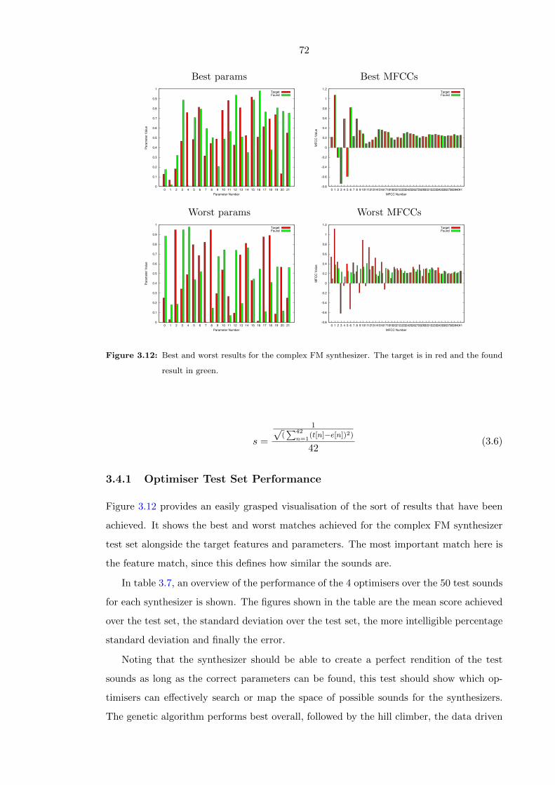
72

Best params Best MFCCs

0

0.1

0.2

0.3

0.4

0.5

0.6

0.7

0.8

0.9

1

0 1 2 3 4 5 6 7 8 9 10 11 12 13 14 15 16 17 18 19 20 21

Para

mete

r V

alu

e

Parameter Number

TargetFound

-0.8

-0.6

-0.4

-0.2

0

0.2

0.4

0.6

0.8

1

1.2

0 1 2 3 4 5 6 7 8 9 1011121314151617181920212223242526272829303132333435363738394041

MF

CC

Valu

e

MFCC Number

TargetFound

Worst params Worst MFCCs

0

0.1

0.2

0.3

0.4

0.5

0.6

0.7

0.8

0.9

1

0 1 2 3 4 5 6 7 8 9 10 11 12 13 14 15 16 17 18 19 20 21

Para

mete

r V

alu

e

Parameter Number

TargetFound

-0.8

-0.6

-0.4

-0.2

0

0.2

0.4

0.6

0.8

1

1.2

0 1 2 3 4 5 6 7 8 9 1011121314151617181920212223242526272829303132333435363738394041

MF

CC

Valu

e

MFCC Number

TargetFound

Figure 3.12: Best and worst results for the complex FM synthesizer. The target is in red and the found

result in green.

s =

1√(∑42

n=1(t[n]−e[n])2)

42(3.6)

3.4.1 Optimiser Test Set Performance

Figure 3.12 provides an easily grasped visualisation of the sort of results that have been

achieved. It shows the best and worst matches achieved for the complex FM synthesizer

test set alongside the target features and parameters. The most important match here is

the feature match, since this defines how similar the sounds are.

In table 3.7, an overview of the performance of the 4 optimisers over the 50 test sounds

for each synthesizer is shown. The figures shown in the table are the mean score achieved

over the test set, the standard deviation over the test set, the more intelligible percentage

standard deviation and finally the error.

Noting that the synthesizer should be able to create a perfect rendition of the test

sounds as long as the correct parameters can be found, this test should show which op-

timisers can effectively search or map the space of possible sounds for the synthesizers.

The genetic algorithm performs best overall, followed by the hill climber, the data driven

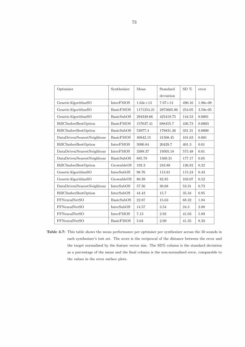
73

Optimiser Synthesizer Mean Standard SD % error

deviation

GeneticAlgorithmSO InterFMOS 1.63e+13 7.97+13 490.16 1.96e-08

GeneticAlgorithmSO BasicFMOS 1171254.21 2975605.86 254.05 3.59e-05

GeneticAlgorithmSO BasicSubOS 294349.66 425419.75 144.53 0.0001

HillClimberBestOption BasicFMOS 157637.41 688455.7 436.73 0.0003

HillClimberBestOption BasicSubOS 53977.4 178831.26 331.31 0.0008

DataDrivenNearestNeighbour BasicFMOS 40842.15 41508.45 101.63 0.001

HillClimberBestOption InterFMOS 5090.84 20429.7 401.3 0.01

DataDrivenNearestNeighbour InterFMOS 3389.37 19505.18 575.48 0.01

DataDrivenNearestNeighbour BasicSubOS 885.78 1569.31 177.17 0.05

HillClimberBestOption GrowableOS 192.3 243.88 126.82 0.22

GeneticAlgorithmSO InterSubOS 98.76 113.81 115.24 0.43

GeneticAlgorithmSO GrowableOS 80.39 82.85 103.07 0.52

DataDrivenNearestNeighbour InterSubOS 57.56 30.68 53.31 0.73

HillClimberBestOption InterSubOS 44.43 15.7 35.34 0.95

FFNeuralNetSO BasicSubOS 22.87 15.63 68.32 1.84

FFNeuralNetSO InterSubOS 14.57 3.54 24.3 2.88

FFNeuralNetSO InterFMOS 7.13 2.92 41.03 5.89

FFNeuralNetSO BasicFMOS 5.04 2.09 41.35 8.33

Table 3.7: This table shows the mean performance per optimiser per synthesizer across the 50 sounds in

each synthesizer’s test set. The score is the reciprocal of the distance between the error and

the target normalised by the feature vector size. The SD% column is the standard deviation

as a percentage of the mean and the final column is the non-normalised error, comparable to

the values in the error surface plots.

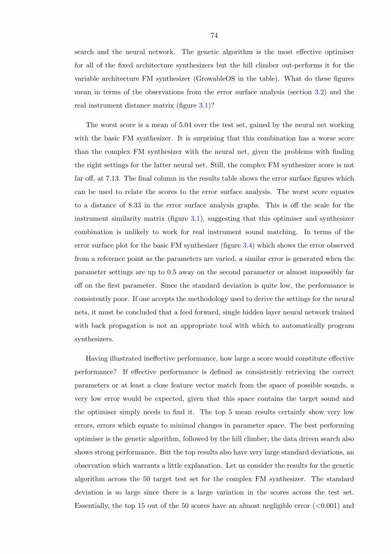
74

search and the neural network. The genetic algorithm is the most effective optimiser

for all of the fixed architecture synthesizers but the hill climber out-performs it for the

variable architecture FM synthesizer (GrowableOS in the table). What do these figures

mean in terms of the observations from the error surface analysis (section 3.2) and the

real instrument distance matrix (figure 3.1)?

The worst score is a mean of 5.04 over the test set, gained by the neural net working

with the basic FM synthesizer. It is surprising that this combination has a worse score

than the complex FM synthesizer with the neural net, given the problems with finding

the right settings for the latter neural net. Still, the complex FM synthesizer score is not

far off, at 7.13. The final column in the results table shows the error surface figures which

can be used to relate the scores to the error surface analysis. The worst score equates

to a distance of 8.33 in the error surface analysis graphs. This is off the scale for the

instrument similarity matrix (figure 3.1), suggesting that this optimiser and synthesizer

combination is unlikely to work for real instrument sound matching. In terms of the

error surface plot for the basic FM synthesizer (figure 3.4) which shows the error observed

from a reference point as the parameters are varied, a similar error is generated when the

parameter settings are up to 0.5 away on the second parameter or almost impossibly far

off on the first parameter. Since the standard deviation is quite low, the performance is

consistently poor. If one accepts the methodology used to derive the settings for the neural

nets, it must be concluded that a feed forward, single hidden layer neural network trained

with back propagation is not an appropriate tool with which to automatically program

synthesizers.

Having illustrated ineffective performance, how large a score would constitute effective

performance? If effective performance is defined as consistently retrieving the correct

parameters or at least a close feature vector match from the space of possible sounds, a

very low error would be expected, given that this space contains the target sound and

the optimiser simply needs to find it. The top 5 mean results certainly show very low

errors, errors which equate to minimal changes in parameter space. The best performing

optimiser is the genetic algorithm, followed by the hill climber; the data driven search also

shows strong performance. But the top results also have very large standard deviations, an

observation which warrants a little explanation. Let us consider the results for the genetic

algorithm across the 50 target test set for the complex FM synthesizer. The standard

deviation is so large since there is a large variation in the scores across the test set.

Essentially, the top 15 out of the 50 scores have an almost negligible error (<0.001) and

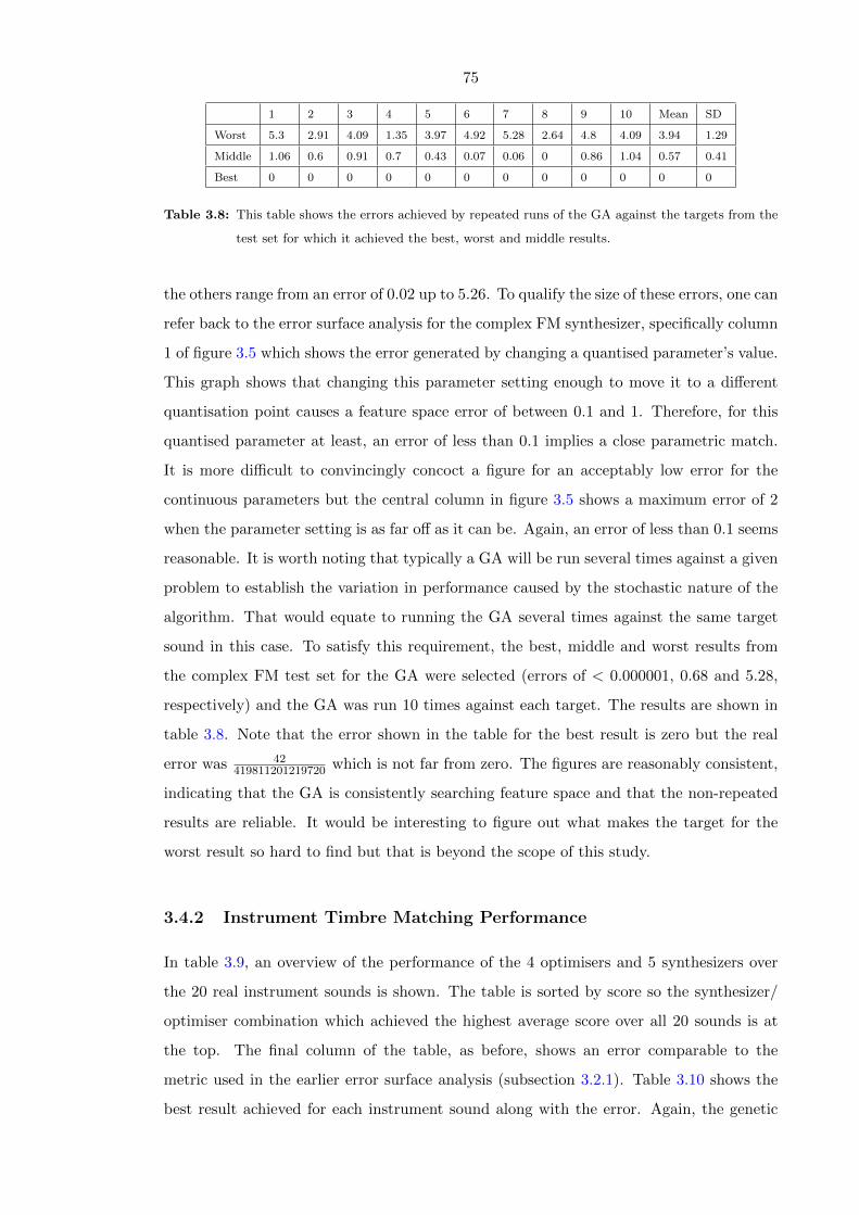
75

1 2 3 4 5 6 7 8 9 10 Mean SD

Worst 5.3 2.91 4.09 1.35 3.97 4.92 5.28 2.64 4.8 4.09 3.94 1.29

Middle 1.06 0.6 0.91 0.7 0.43 0.07 0.06 0 0.86 1.04 0.57 0.41

Best 0 0 0 0 0 0 0 0 0 0 0 0

Table 3.8: This table shows the errors achieved by repeated runs of the GA against the targets from the

test set for which it achieved the best, worst and middle results.

the others range from an error of 0.02 up to 5.26. To qualify the size of these errors, one can

refer back to the error surface analysis for the complex FM synthesizer, specifically column

1 of figure 3.5 which shows the error generated by changing a quantised parameter’s value.

This graph shows that changing this parameter setting enough to move it to a different

quantisation point causes a feature space error of between 0.1 and 1. Therefore, for this

quantised parameter at least, an error of less than 0.1 implies a close parametric match.

It is more difficult to convincingly concoct a figure for an acceptably low error for the

continuous parameters but the central column in figure 3.5 shows a maximum error of 2

when the parameter setting is as far off as it can be. Again, an error of less than 0.1 seems

reasonable. It is worth noting that typically a GA will be run several times against a given

problem to establish the variation in performance caused by the stochastic nature of the

algorithm. That would equate to running the GA several times against the same target

sound in this case. To satisfy this requirement, the best, middle and worst results from

the complex FM test set for the GA were selected (errors of < 0.000001, 0.68 and 5.28,

respectively) and the GA was run 10 times against each target. The results are shown in

table 3.8. Note that the error shown in the table for the best result is zero but the real

error was 42419811201219720 which is not far from zero. The figures are reasonably consistent,

indicating that the GA is consistently searching feature space and that the non-repeated

results are reliable. It would be interesting to figure out what makes the target for the

worst result so hard to find but that is beyond the scope of this study.

3.4.2 Instrument Timbre Matching Performance

In table 3.9, an overview of the performance of the 4 optimisers and 5 synthesizers over

the 20 real instrument sounds is shown. The table is sorted by score so the synthesizer/

optimiser combination which achieved the highest average score over all 20 sounds is at

the top. The final column of the table, as before, shows an error comparable to the

metric used in the earlier error surface analysis (subsection 3.2.1). Table 3.10 shows the

best result achieved for each instrument sound along with the error. Again, the genetic

76

Optimiser Synthesizer Mean Standard SD% Error

deviation

GeneticAlgorithmSO InterFMOS 22.9702 6.2617 27.2601 1.828

GeneticAlgorithmSO InterSubOS 21.0570 4.4694 21.2255 1.995

DataDrivenNearestNeighbour BasicSubOS 20.9126 3.5917 17.1749 2.008

DataDrivenNearestNeighbour InterFMOS 20.7831 5.1740 24.8950 2.021

DataDrivenNearestNeighbour InterSubOS 20.0827 3.5742 17.7974 2.091

GeneticAlgorithmSO BasicSubOS 19.7633 3.6499 18.4679 2.125

HillClimberBestOption BasicSubOS 19.3550 3.6726 18.9750 2.170

HillClimberBestOption GrowableOS 15.1654 3.4224 22.5669 2.769

HillClimberBestOption InterSubOS 14.7632 3.4241 23.1937 2.845

GeneticAlgorithmSO GrowableOS 12.7828 2.1272 16.6414 3.286

HillClimberBestOption InterFMOS 12.4737 3.6924 29.6018 3.367

DataDrivenNearestNeighbour BasicFMOS 10.5969 1.7464 16.4808 3.963

GeneticAlgorithmSO BasicFMOS 10.5942 1.7434 16.4561 3.964

FFNeuralNetSO BasicSubOS 10.3134 2.1984 21.3157 4.072

FFNeuralNetSO InterSubOS 9.9958 1.7921 17.9287 4.202

HillClimberBestOption BasicFMOS 9.1044 2.0576 22.5998 4.613

FFNeuralNetSO InterFMOS 7.9552 1.8834 23.6752 5.280

FFNeuralNetSO BasicFMOS 6.0991 1.9064 31.2576 6.886

Table 3.9: This table shows the mean performance per optimiser, per synthesizer across the 20 real

instrument sounds. The data is sorted by score so the best performing synthesizer/ optimiser

combinations appear at the top.

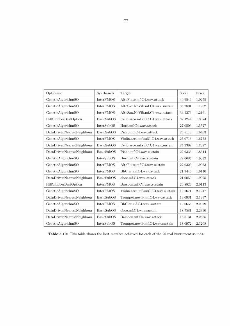
77

Optimiser Synthesizer Target Score Error

GeneticAlgorithmSO InterFMOS AltoFlute.mf.C4.wav attack 40.9549 1.0255

GeneticAlgorithmSO InterFMOS AltoSax.NoVib.mf.C4.wav sustain 35.2891 1.1902

GeneticAlgorithmSO InterFMOS AltoSax.NoVib.mf.C4.wav attack 34.5376 1.2161

HillClimberBestOption BasicSubOS Cello.arco.mf.sulC.C4.wav attack 32.1244 1.3074

GeneticAlgorithmSO InterSubOS Horn.mf.C4.wav attack 27.0503 1.5527

DataDrivenNearestNeighbour BasicSubOS Piano.mf.C4.wav attack 25.5118 1.6463

GeneticAlgorithmSO InterFMOS Violin.arco.mf.sulG.C4.wav attack 25.0713 1.6752

DataDrivenNearestNeighbour BasicSubOS Cello.arco.mf.sulC.C4.wav sustain 24.2392 1.7327

DataDrivenNearestNeighbour BasicSubOS Piano.mf.C4.wav sustain 22.9333 1.8314

GeneticAlgorithmSO InterSubOS Horn.mf.C4.wav sustain 22.0686 1.9032

GeneticAlgorithmSO InterFMOS AltoFlute.mf.C4.wav sustain 22.0323 1.9063

GeneticAlgorithmSO InterFMOS BbClar.mf.C4.wav attack 21.9440 1.9140

DataDrivenNearestNeighbour BasicSubOS oboe.mf.C4.wav attack 21.0050 1.9995

HillClimberBestOption InterFMOS Bassoon.mf.C4.wav sustain 20.8823 2.0113

GeneticAlgorithmSO InterFMOS Violin.arco.mf.sulG.C4.wav sustain 19.7671 2.1247

DataDrivenNearestNeighbour BasicSubOS Trumpet.novib.mf.C4.wav attack 19.0931 2.1997

GeneticAlgorithmSO InterFMOS BbClar.mf.C4.wav sustain 19.0656 2.2029

DataDrivenNearestNeighbour BasicSubOS oboe.mf.C4.wav sustain 18.7581 2.2390

DataDrivenNearestNeighbour BasicSubOS Bassoon.mf.C4.wav attack 18.6131 2.2565

GeneticAlgorithmSO InterSubOS Trumpet.novib.mf.C4.wav sustain 18.0972 2.3208

Table 3.10: This table shows the best matches achieved for each of the 20 real instrument sounds.

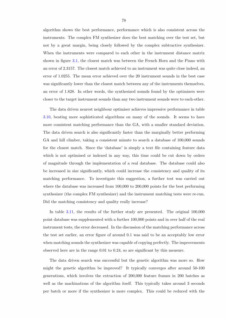
78

algorithm shows the best performance, performance which is also consistent across the

instruments. The complex FM synthesizer does the best matching over the test set, but

not by a great margin, being closely followed by the complex subtractive synthesizer.

When the instruments were compared to each other in the instrument distance matrix

shown in figure 3.1, the closest match was between the French Horn and the Piano with

an error of 2.3157. The closest match achieved to an instrument was quite close indeed, an

error of 1.0255. The mean error achieved over the 20 instrument sounds in the best case

was significantly lower than the closest match between any of the instruments themselves,

an error of 1.828. In other words, the synthesized sounds found by the optimisers were

closer to the target instrument sounds than any two instrument sounds were to each-other.

The data driven nearest neighbour optimiser achieves impressive performance in table

3.10, beating more sophisticated algorithms on many of the sounds. It seems to have

more consistent matching performance than the GA, with a smaller standard deviation.

The data driven search is also significantly faster than the marginally better performing

GA and hill climber, taking a consistent minute to search a database of 100,000 sounds

for the closest match. Since the ‘database’ is simply a text file containing feature data

which is not optimised or indexed in any way, this time could be cut down by orders

of magnitude through the implementation of a real database. The database could also

be increased in size significantly, which could increase the consistency and quality of its

matching performance. To investigate this suggestion, a further test was carried out

where the database was increased from 100,000 to 200,000 points for the best performing

synthesizer (the complex FM synthesizer) and the instrument matching tests were re-run.

Did the matching consistency and quality really increase?

In table 3.11, the results of the further study are presented. The original 100,000

point database was supplemented with a further 100,000 points and in over half of the real

instrument tests, the error decreased. In the discussion of the matching performance across

the test set earlier, an error figure of around 0.1 was said to be an acceptably low error

when matching sounds the synthesizer was capable of copying perfectly. The improvements

observed here are in the range 0.01 to 0.24, so are significant by this measure.

The data driven search was successful but the genetic algorithm was more so. How

might the genetic algorithm be improved? It typically converges after around 50-100

generations, which involves the extraction of 200,000 feature frames in 200 batches as

well as the machinations of the algorithm itself. This typically takes around 3 seconds

per batch or more if the synthesizer is more complex. This could be reduced with the

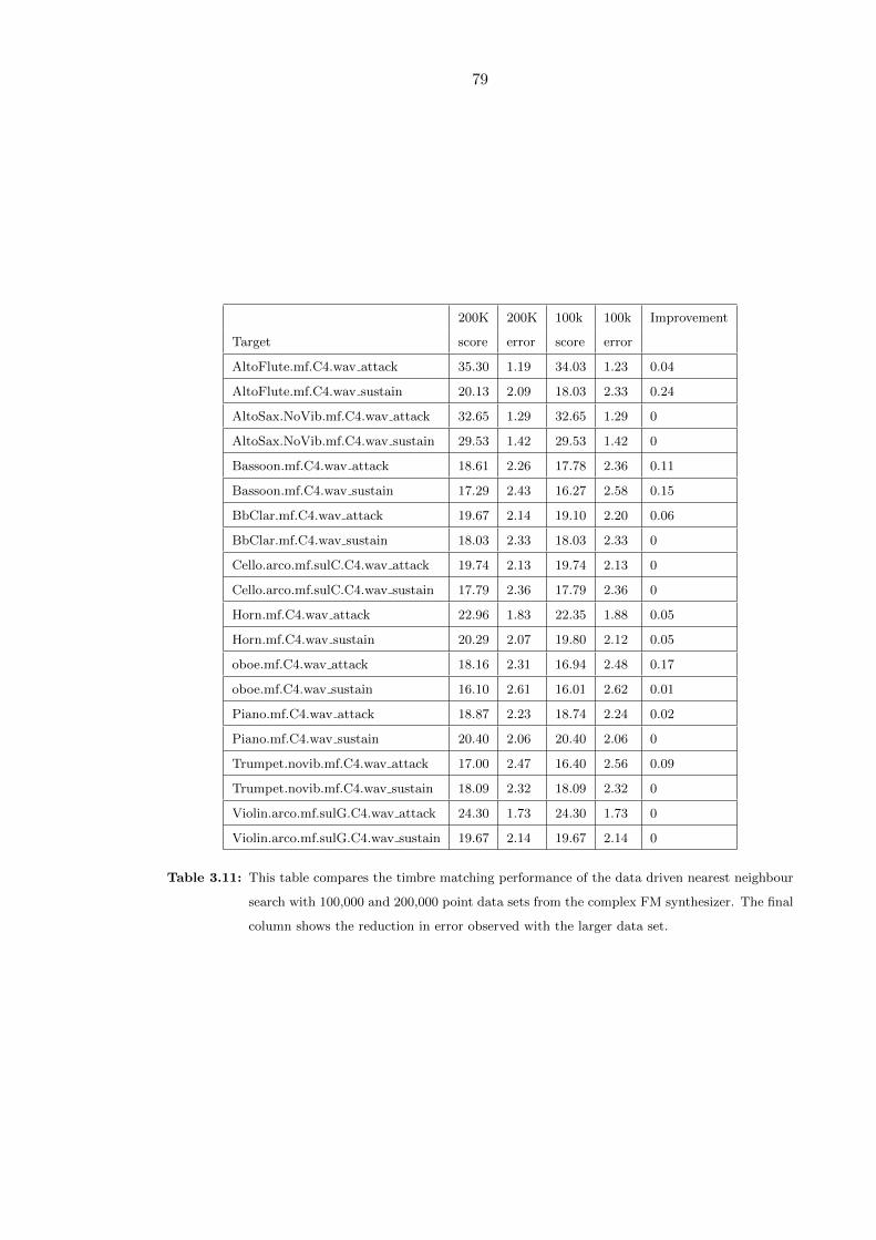
79

200K 200K 100k 100k Improvement

Target score error score error

AltoFlute.mf.C4.wav attack 35.30 1.19 34.03 1.23 0.04

AltoFlute.mf.C4.wav sustain 20.13 2.09 18.03 2.33 0.24

AltoSax.NoVib.mf.C4.wav attack 32.65 1.29 32.65 1.29 0

AltoSax.NoVib.mf.C4.wav sustain 29.53 1.42 29.53 1.42 0

Bassoon.mf.C4.wav attack 18.61 2.26 17.78 2.36 0.11

Bassoon.mf.C4.wav sustain 17.29 2.43 16.27 2.58 0.15

BbClar.mf.C4.wav attack 19.67 2.14 19.10 2.20 0.06

BbClar.mf.C4.wav sustain 18.03 2.33 18.03 2.33 0

Cello.arco.mf.sulC.C4.wav attack 19.74 2.13 19.74 2.13 0

Cello.arco.mf.sulC.C4.wav sustain 17.79 2.36 17.79 2.36 0

Horn.mf.C4.wav attack 22.96 1.83 22.35 1.88 0.05

Horn.mf.C4.wav sustain 20.29 2.07 19.80 2.12 0.05

oboe.mf.C4.wav attack 18.16 2.31 16.94 2.48 0.17

oboe.mf.C4.wav sustain 16.10 2.61 16.01 2.62 0.01

Piano.mf.C4.wav attack 18.87 2.23 18.74 2.24 0.02

Piano.mf.C4.wav sustain 20.40 2.06 20.40 2.06 0

Trumpet.novib.mf.C4.wav attack 17.00 2.47 16.40 2.56 0.09

Trumpet.novib.mf.C4.wav sustain 18.09 2.32 18.09 2.32 0

Violin.arco.mf.sulG.C4.wav attack 24.30 1.73 24.30 1.73 0

Violin.arco.mf.sulG.C4.wav sustain 19.67 2.14 19.67 2.14 0

Table 3.11: This table compares the timbre matching performance of the data driven nearest neighbour

search with 100,000 and 200,000 point data sets from the complex FM synthesizer. The final

column shows the reduction in error observed with the larger data set.

80

Target Standard Hybrid Standard Hybrid Error

GA score GA GA error GA difference

score error

AltoFlute.mf.C4.wav attack 40.9549 35.3057 1.0255 1.1896 0.1641

AltoFlute.mf.C4.wav sustain 22.0323 20.5850 1.9063 2.0403 0.1340

AltoSax.NoVib.mf.C4.wav attack 34.5376 32.6473 1.2161 1.2865 0.0704

AltoSax.NoVib.mf.C4.wav sustain 35.2891 32.5919 1.1902 1.2887 0.0985

Bassoon.mf.C4.wav attack 18.4056 23.0549 2.2819 1.8217 -0.4602

Bassoon.mf.C4.wav sustain 17.4296 19.5440 2.4097 2.1490 -0.2607

BbClar.mf.C4.wav attack 21.9440 19.6708 1.9140 2.1351 0.2212

BbClar.mf.C4.wav sustain 19.0656 19.6745 2.2029 2.1347 -0.0682

Cello.arco.mf.sulC.C4.wav attack 21.0522 23.4298 1.9950 1.7926 -0.2025

Cello.arco.mf.sulC.C4.wav sustain 21.9489 18.8694 1.9135 2.2258 0.3123

Horn.mf.C4.wav attack 22.9452 27.2126 1.8304 1.5434 -0.2870

Horn.mf.C4.wav sustain 21.2800 22.8407 1.9737 1.8388 -0.1349

oboe.mf.C4.wav attack 19.5410 18.1563 2.1493 2.3132 0.1639

oboe.mf.C4.wav sustain 18.6582 16.8630 2.2510 2.4907 0.2396

Piano.mf.C4.wav attack 21.2228 19.1744 1.9790 2.1904 0.2114

Piano.mf.C4.wav sustain 22.3547 22.6377 1.8788 1.8553 -0.0235

Trumpet.novib.mf.C4.wav attack 18.1214 19.4593 2.3177 2.1583 -0.1594

Trumpet.novib.mf.C4.wav sustain 17.7829 18.0937 2.3618 2.3212 -0.0406

Violin.arco.mf.sulG.C4.wav attack 25.0713 24.3025 1.6752 1.7282 0.0530

Violin.arco.mf.sulG.C4.wav sustain 19.7671 19.6673 2.1247 2.1355 0.0108

Table 3.12: This table compares the standard GA which starts with a random population to the hybrid

GA which starts with a population derived from a data driven search.

implementation of a multi-threaded algorithm, probably to 1numberofCPUcores but it will

never match the speed of the data driven approach, even with the latter in its unoptimised

form. Therefore a hybrid approach is proposed, where the initial population for the genetic

algorithm is generated by finding the 1000 closest matches to the target using the data

driven search. This system was implemented and it was run against the 20 instrument

sounds using the complex FM synthesizer. The results of the standard GA and the hybrid

GA are compared in table 3.12. The results do not show the hybrid GA to be superior, it

performs worse about as many times as it performs better.

3.4.3 Conclusion

Five sound synthesis algorithms have been described and their behaviour in feature space

as their parameter settings are varied has been investigated. Five optimisation techniques

81

have been described and their performance at the problem of eliciting appropriate pa-

rameter settings for the sound synthesis algorithms has been extensively tested. The best

performing optimisation technique was the genetic algorithm, which searches well and

with reasonable consistency over all of the fixed architecture sound synthesizers. It was

not the best performer in the search of the space of sounds that can be generated by

a variable architecture synthesizer, however, being beaten by the more conservative hill

climber. The feed forward neural network failed nearly completely at the task. The greedy

search offered by the data driven approach was shown to be more efficient than the ge-

netic algorithm as well as having nearly comparable search performance in several cases.

Increasing the greed of this search by using a bigger data set was shown to be effective in

an initial test. The hybrid form of the genetic algorithm and the greedy search was not

shown to have better performance in an initial test. Regarding the eliciting of optimal

parameter settings for the synthesizers for the matching of real instrument timbres, the

complex FM synthesis algorithm, similar to that found in the Yamaha DX7, was found

to be superior to analog-style subtractive algorithms overall. However, the subtractive

algorithms still performed well and better than FM in some cases such as the Violin and

French Horn sounds. There was no apparent pattern at work here, e.g. the subtractive

synthesizers being better at making string sounds.

The next chapter is about SynthBot. SynthBot is an automatic VSTi sound synthesizer

programmer which is implemented based partly on the results of this study.

82

Chapter 4

Sound Synthesis Space

Exploration as a Studio Tool:

SynthBot

This chapter presents the first of three applications of automatic sound synthesizer pro-

gramming: SynthBot. SynthBot uses a genetic algorithm to search for parameter settings

which cause any synthesizer available in the industry standard VSTi format to emit a

sound which matches as closely as possible a target sound. The motivation for the devel-

opment of SynthBot is described as the apparent difficulty involved in programming many

synthesizers. Other methods provided by commercial synthesizer vendors for facilitating

synthesizer programming are described, including applications of machine learning. The

technical implementation of SynthBot is detailed, where SynthBot acts as a VST host

implemented in the Java language, using the Java Native Interface to load and interact

with natively compiled VST plug-ins. The genetic algorithm is described and technically

evaluated in terms of its speed and search capabilities using the freely available mdaJX10

and mdaDX10 synthesizers. A method is outlined for experimentally evaluating SynthBot,

where the synthesizer programming abilities of experienced humans can be compared to

those of SynthBot. The experiment was conducted using 10 participants and SynthBot

performed better than the humans, according to its own method of measuring distances

between sounds with the MFCC feature vector. The parameter varying behaviour of the

human and machine programmers during the trial was also recorded and this is compared.

The chapter concludes by recounting the current status of the SynthBot project.

83

4.1 Introduction

This section provides some background and motivation for the work reported in this chap-

ter. The difficulty of programming synthesizers is discussed; previous research applying

machine learning to the problem is reviewed; finally, the motivation for the construction

of SynthBot is provided.

4.1.1 The Difficulty of Programming Synthesizers

As sound synthesis algorithms increase in complexity, there is typically an associated in-

crease in the number of parameters required to control them and the difficulty of specifying

values for these parameters. The increased capabilities offered by more complex synthesis

algorithms were aptly illustrated in chapter 3, where the complex FM synthesizer proved to

be the most flexible timbre generator yet had a large number of non-intuitive parameters.

Also, certain synthesis methods can be described as less intuitive than others, for example

the Yamaha DX7 was informally known for being difficult to program, compared to the

subtractive synthesis based analog designs that had come before it [124]. The parameters

on the DX7 had new names (e.g. modulation index instead of filter cut off) and it was

not clear what they were likely to do; the user interface was somewhat unfriendly, with

its simple two line digital LCD readout. Compare this to a bank of easily manipulated

knobs and sliders as found on the analog synthesizers which the DX7 aimed to supersede.

Moving forward in time to the present day, digital synthesizers can have a huge number

of parameters, for example the current version of Native Instruments’ FM8 synthesizer has

1093 parameters [54]. Even with a user interface which is far in advance of the early FM

synthesizers, creating sounds that are more than mild adjustments of the presets can be

a challenge. Indeed, the manufacturers of these synthesizers have acknowledged this com-

plexity via the provision of large banks of preset sounds, along with new, category-driven

user interfaces for finding the desired preset. Examples of this are Native Instruments’

‘KoreSound Browser’ and Arturia’s ‘Analog Factory’. The ‘KoreSound Browser’ uses a

category browsing interface, where the user might select ‘Bass sound’, ‘Analog’ and ‘Cold’,

for example. [56]. Arturia provide a similar interface where the user might select ‘Lead’

and ‘Dark’ [4]. If it was possible to easily create a desired sound from scratch, there would

be no need for such libraries.

84

4.1.2 Applying Machine Learning to Synthesizer Programming

The use of machine learning techniques for sound synthesizer programming appears regu-

larly in the computer music literature. An early example used FM synthesis and a genetic

algorithm to achieve tone matching [48]. FM synthesis is combined with GA programmers

several times in the literature (e.g. [67, 2, 142], but other synthesis algorithms have been

tried, e.g. noise band synthesis [18] and subtractive synthesis [143]. The problem with

these systems, a problem which the system presented here aims to solve, is that they are

not typically available for public consumption 1. Further, if they are available, they do not

integrate with existing tools used by musicians, even in a simple way such as via MIDI.

Moving away from the computer music literature, what have commercial manufacturers

provided in terms of applied machine intelligence, that allows the user to escape from banks

of categorised presets? There appear to have been only two clear examples of a genetic

algorithm being deployed in a commercial music system: Dahlstedt’s Nord Modular G2

‘Patch Mutator’ and the work of Heise et al with VST instruments [30, 44].

The Nord Modular G2 is a hardware synthesizer which implements virtual modular

synthesis and is programmed using graphical patching software on a standard PC/ Mac.

Part of this software is an interactive genetic algorithm referred to as the ‘Patch Mutator’

[30]. This system allows the user to interactively evolve the parameter settings for patches

by breeding and mutation, where the user provides the fitness judgement by choosing

which of the generated sounds to keep and which to discard. It does not provide the

capability to add or remove modules to the patch, so is limited to parametric exploration

of fixed architecture synthesis algorithms. The work reported in chapter 3 suggests that if

the approach is to gradually mutate and breed the sounds, that many thousands of sounds

must be auditioned before a target sound can be found. This is not feasible when a human

is providing the fitness measure as there is simply not enough time.

The work of Heise et al. reported in 2009 resulted in a general purpose VST instrument

programmer [44], which is the same goal as that for the work presented here. However, it

is worth noting that the work presented in this chapter was first published in 2008 [144].

One other related example for consideration is ‘The Mutator’, described in the manual

for Native Instruments’ Absynth 5 synthesizer [55]. This system attempts to interpolate

between patches chosen by the user by manipulating the character of the sound. The

system must have some way of translating from combinations of weighted categories to

synthesis parameters, but it is not clear how this is done. It bears a resemblance to work

1Chinen’s system is available under an open source license [18]

85

by Johnson and Gounaropoulos where neural nets were used to learn the mapping between

synthesis parameters and timbre words such as thick, metallic and woody based on user

derived training sets, which enabled the words to be used to program the synthesizer [60].

It is also possible that it uses a similar system to Bencina’s Metasurface [7].

To return to the body of existing research work focused on the automated sound syn-

thesizer programming problem, a key question is how to judge sound similarity. Many

opt for an error measure obtained by comparing the power spectra of the candidate and

target sounds, an approach which does indeed reward similar sounds. One problem with

the power spectrum is its brittleness; if the same instrument plays two differently pitched

notes, there will be a large error between the power spectra even if the notes could clearly

be identified by a human user as having been played using the same instrument. It follows

that an improvement in the error measure will be gained by considering the human per-

ception of timbre. This is addressed in some of the research, where perceptually informed

measures such as the spectral centroid are used, e.g. [67], [44].

4.1.3 The Need for SynthBot

So the problem can be reduced to the fact that sound synthesizers are hard to program.

Work by other researchers shows that GAs can be used to find settings for synthesizers

to enable tone matching and the work reported in chapter 3 shows that other methods

might also be employed, with varying degrees of success but that the GA is the best

option. In chapter 2, the importance of considering human perception is established.

Finally, previous to the work reported here, which was first published in 2008, there has

not been a non-interactive GA which is capable of programming commercially available

synthesizers. SynthBot aims to solve these problems and to provide a new studio tool to

musicians.

4.2 Implementation

In this section, the implementation of the SynthBot software is described; specifically, the

VST and Java background technologies, the sound synthesis algorithms used for evalua-

tion, the parameter search method and the set-up for the experimental evaluation.

4.2.1 Background Technologies

Virtual Studio Technology or VST is a standard developed by Steinberg which allows

developers to construct audio effect and synthesis plug-ins that can be used within audio

86

workstation software such as Cubase [115]. The workstation software in this case is referred

to as a VST host. A developer simply implements the VST standard in their plug-in and

it can then be loaded by any host which supports that version of the plug-in standard.

A VST instrument or VSTi is slightly different from a basic VST in that it can receive

MIDI data from the host; this allows it to behave like a synthesizer, playing notes and

varying its sound in response to MIDI. A large range of VSTi compatible synthesizers have

been developed; a database of available plug-ins is maintained by KVR audio [53]. VST

plug-ins are provided as natively compiled, dynamically loadable modules; either DLL,

dylib or .so for Windows, Mac and Linux, respectively. As such, it can be considered to

be a cross platform standard.

SynthBot is implemented using the Java and C++ programming languages as a cross

platform, standalone application running on Windows, MacOSX and GNU/ Linux. Syn-

thBot acts as a VST host, loading plug-ins, manipulating their parameter settings and

using them to generate audio signals. In order to bridge the Java Virtual Machine with

the natively compiled VSTi plug-in modules, the Java Native Interface (JNI) is used [72].

The VST host component of SynthBot (JVstHost) was developed mainly by Martin Roth

and is available under an open source license [103]; the version of the SynthBot software

used for the tests presented here was coded by Matthew Yee-King.

4.2.2 Sound Synthesis

Since the system is compatible with any VSTi plug-in, it is capable of working with any

sound synthesis algorithm available in this plug-in format. In the evaluations presented

here, the freely available mda synthesizer plug-ins mdaDX10 and mdaJX10 were used

[62]. The mdaDX10 is a single modulator FM synthesizer with 16 parameters and the

mdaJX10 is a subtractive synthesizer with 2 tuned and one noise oscillator, controlled via

40 parameters. The parameters for these synthesizers are shown in tables 4.1 and 4.2.

4.2.3 Automatic Parameter Search

In the VSTi standard, each synthesizer parameter is represented as a real number (in-

ternally stored as a 32 bit float) between zero and one, inclusive. Therefore a search

algorithm will be searching for an array of parameter settings with a length equal to the

number of parameters. Modern synthesizers may have hundreds of parameters, making

the search space high dimensional. A genetic algorithm is used to search the space of

possible parameter settings for the synthesizer for those settings which cause it to emit as

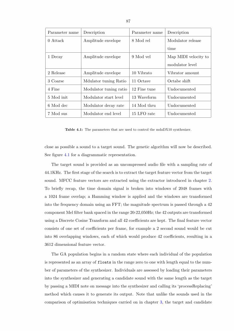
87

Parameter name Description Parameter name Description

0 Attack Amplitude envelope 8 Mod rel Modulator release

time

1 Decay Amplitude envelope 9 Mod vel Map MIDI velocity to

modulator level

2 Release Amplitude envelope 10 Vibrato Vibrator amount

3 Coarse Mdulator tuning Ratio 11 Octave Octabe shift

4 Fine Modulator tuning ratio 12 Fine tune Undocumented

5 Mod init Modulator start level 13 Waveform Undocumented

6 Mod dec Modulator decay rate 14 Mod thru Undocumented

7 Mod sus Modulator end level 15 LFO rate Undocumented

Table 4.1: The parameters that are used to control the mdaDX10 synthesizer.

close as possible a sound to a target sound. The genetic algorithm will now be described.

See figure 4.1 for a diagrammatic representation.

The target sound is provided as an uncompressed audio file with a sampling rate of

44.1KHz. The first stage of the search is to extract the target feature vector from the target

sound. MFCC feature vectors are extracted using the extractor introduced in chapter 2.

To briefly recap, the time domain signal is broken into windows of 2048 frames with

a 1024 frame overlap; a Hamming window is applied and the windows are transformed

into the frequency domain using an FFT; the magnitude spectrum is passed through a 42

component Mel filter bank spaced in the range 20-22,050Hz; the 42 outputs are transformed

using a Discrete Cosine Transform and all 42 coefficients are kept. The final feature vector

consists of one set of coefficients per frame, for example a 2 second sound would be cut

into 86 overlapping windows, each of which would produce 42 coefficients, resulting in a

3612 dimensional feature vector.

The GA population begins in a random state where each individual of the population

is represented as an array of floats in the range zero to one with length equal to the num-

ber of parameters of the synthesizer. Individuals are assessed by loading their parameters

into the synthesizer and generating a candidate sound with the same length as the target

by passing a MIDI note on message into the synthesizer and calling its ‘processReplacing’

method which causes it to generate its output. Note that unlike the sounds used in the

comparison of optimisation techniques carried on in chapter 3, the target and candidate

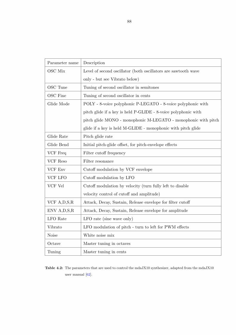
88

Parameter name Description

OSC Mix Level of second oscillator (both oscillators are sawtooth wave

only - but see Vibrato below)

OSC Tune Tuning of second oscillator in semitones

OSC Fine Tuning of second oscillator in cents

Glide Mode POLY - 8-voice polyphonic P-LEGATO - 8-voice polyphonic with

pitch glide if a key is held P-GLIDE - 8-voice polyphonic with

pitch glide MONO - monophonic M-LEGATO - monophonic with pitch

glide if a key is held M-GLIDE - monophonic with pitch glide

Glide Rate Pitch glide rate

Glide Bend Initial pitch-glide offset, for pitch-envelope effects

VCF Freq Filter cutoff frequency

VCF Reso Filter resonance

VCF Env Cutoff modulation by VCF envelope

VCF LFO Cutoff modulation by LFO

VCF Vel Cutoff modulation by velocity (turn fully left to disable

velocity control of cutoff and amplitude)

VCF A,D,S,R Attack, Decay, Sustain, Release envelope for filter cutoff

ENV A,D,S,R Attack, Decay, Sustain, Release envelope for amplitude

LFO Rate LFO rate (sine wave only)

Vibrato LFO modulation of pitch - turn to left for PWM effects

Noise White noise mix

Octave Master tuning in octaves

Tuning Master tuning in cents

Table 4.2: The parameters that are used to control the mdaJX10 synthesizer, adapted from the mdaJX10

user manual [62].

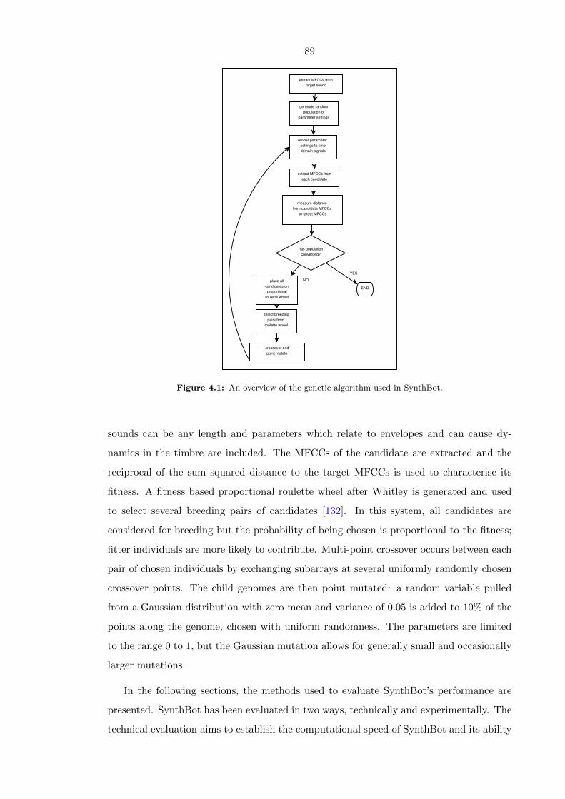
89

��

extract MFCCs from

target sound

generate random

population of

parameter settings

render parameter

settings to time

domain signals

extract MFCCs from

each candidate

measure distance

from candidate MFCCs

to target MFCCs

place all

candidates on

proportional

roulette wheel

select breeding

pairs from

roulette wheel

crossover and

point mutate

has population

converged?

END

YES

NO

Figure 4.1: An overview of the genetic algorithm used in SynthBot.

sounds can be any length and parameters which relate to envelopes and can cause dy-

namics in the timbre are included. The MFCCs of the candidate are extracted and the

reciprocal of the sum squared distance to the target MFCCs is used to characterise its

fitness. A fitness based proportional roulette wheel after Whitley is generated and used

to select several breeding pairs of candidates [132]. In this system, all candidates are

considered for breeding but the probability of being chosen is proportional to the fitness;

fitter individuals are more likely to contribute. Multi-point crossover occurs between each

pair of chosen individuals by exchanging subarrays at several uniformly randomly chosen

crossover points. The child genomes are then point mutated: a random variable pulled

from a Gaussian distribution with zero mean and variance of 0.05 is added to 10% of the

points along the genome, chosen with uniform randomness. The parameters are limited

to the range 0 to 1, but the Gaussian mutation allows for generally small and occasionally

larger mutations.

In the following sections, the methods used to evaluate SynthBot’s performance are

presented. SynthBot has been evaluated in two ways, technically and experimentally. The

technical evaluation aims to establish the computational speed of SynthBot and its ability

90

to effectively search the space of possible sounds for a given synthesizer. The experi-

mental evaluation aims to establish the superiority or otherwise of SynthBot’s synthesizer

programming abilities over those of experienced human users.

4.3 Technical Evaluation

The first aspect of performance is the speed with which candidate sounds can be assigned

a fitness. This process involves sending the parameters to the synthesizer, rendering its

output for (target sound length) seconds, extracting MFCCs and calculating the reciprocal

of the Euclidean distance to the target feature vector. If the target sound is around one

second long, SynthBot can calculate the fitness of a given candidate in around 10ms with

the mdaJX10 and mdaDX10 synthesizers, assuming two candidates are assessed at the

same time, as can be achieved with a dual core CPU. This is measured on a Thinkpad

T400 laptop with a dual core, 2.53GHz Intel CPU running 64 bit Ubuntu Linux 10.04

and Sun’s 1.6.0 22 32 bit Java runtime (JRE). The 32 bit runtime is used to enable the

loading of 32 bit VST plug-ins by the JRE.

The second aspect of performance is the effectiveness of the search and the number

of fitness assessments required to gain an acceptable match. Following the methodology

described in the previous chapter (3), this is assessed by searching for sounds generated

by the synthesizer itself using known parameter settings. Since the synthesizer should

be capable of generating these sounds, a perfect search algorithm should be capable of

finding the known parameters, assuming the synthesizer cannot make the same sound

using different parameters. At least the search algorithm should find a very close match

for the target MFCCs.

In order to establish that the system is capable of effectively searching the space of

possible parameter settings, the following process was carried out 50 times:

1. A target audio file is rendered using the mdaDX10 synthesizer with random param-

eter settings.

2. The optimiser runs for 100 generations with a population size of 500, using the

random sound as a target.

The optimisation step requires 50,000 fitness assessments (500 genomes, 100 iterations)

which takes approximately 10 minutes, at 10ms per assessment. The fitness is observed

to level out after around 25,000 assessments (50 generations).

91

Figure 4.2: The power spectra of the 3 best matches out of 50 trials, achieved by SynthBot using the

mdaJX10 synthesizer and random sounds. Note that matching was achieved using a different

metric, the MFCC.

Figure 4.3: The power spectra of the 3 middle scoring matches out of 50 trials, achieved by SynthBot

using the mdaJX10 synthesizer and random sounds.

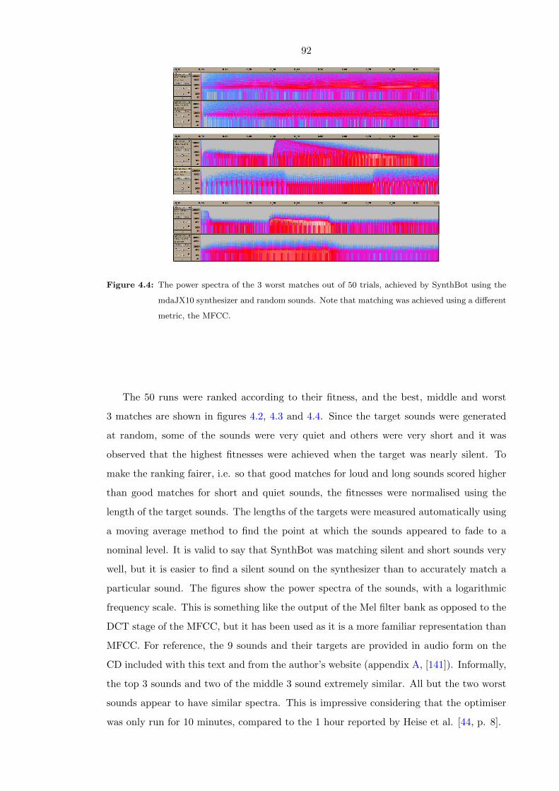
92

Figure 4.4: The power spectra of the 3 worst matches out of 50 trials, achieved by SynthBot using the

mdaJX10 synthesizer and random sounds. Note that matching was achieved using a different

metric, the MFCC.

The 50 runs were ranked according to their fitness, and the best, middle and worst

3 matches are shown in figures 4.2, 4.3 and 4.4. Since the target sounds were generated

at random, some of the sounds were very quiet and others were very short and it was

observed that the highest fitnesses were achieved when the target was nearly silent. To

make the ranking fairer, i.e. so that good matches for loud and long sounds scored higher

than good matches for short and quiet sounds, the fitnesses were normalised using the

length of the target sounds. The lengths of the targets were measured automatically using

a moving average method to find the point at which the sounds appeared to fade to a

nominal level. It is valid to say that SynthBot was matching silent and short sounds very

well, but it is easier to find a silent sound on the synthesizer than to accurately match a

particular sound. The figures show the power spectra of the sounds, with a logarithmic

frequency scale. This is something like the output of the Mel filter bank as opposed to the

DCT stage of the MFCC, but it has been used as it is a more familiar representation than

MFCC. For reference, the 9 sounds and their targets are provided in audio form on the

CD included with this text and from the author’s website (appendix A, [141]). Informally,

the top 3 sounds and two of the middle 3 sound extremely similar. All but the two worst

sounds appear to have similar spectra. This is impressive considering that the optimiser

was only run for 10 minutes, compared to the 1 hour reported by Heise et al. [44, p. 8].

93

4.4 Experimental Evaluation

The experimental evaluation aimed to compare the synthesizer programming abilities of

SynthBot to those of experienced human users. Ten subjects were chosen to be involved in

the experiment. They all had significant past experience of programming synthesizers and

were also experienced computer users. The subjects were asked to carry out the following

tasks:

1. Program the mdaDX10 to make a sound that was generated using the mdaDX10

with known parameters. The sound was a ‘classic’ FM synthesizer sound: a short,

metallic percussion sound.

2. Program the mdaDX10 to make a real instrument sound. The sound was a piano

note.

3. Program the mdaJX10 to make a sound that was generated using the mdaJX10.

The sound was a ‘classic’ analogue synthesizer sound: a rich, sustained tone with

vibrato.

4. Program the mdaJX10 to make a real instrument sound. The sound was a sustained

violin note with minimal modulation.

The experimental procedure was as follows:

1. The plan for the experiment was explained to the subject - they were told what they

would be required to do and how long they would have to do it. They were also told

how to use the software to program the synthesizer and how to listen to the target

and synthesizer sounds.

2. The mdaDX10 synthesizer was loaded and the subject was given five minutes to

freely operate the synthesizer programming interface and to listen to the resulting

sounds.

3. The synthesized target sound was provided to the subject and they were given five

minutes to find the closest possible sound to the target sound. When one minute

remained, they were informed of this so they could recall an earlier setting if nec-

essary. At the end of the synthesizer programming, the resultant parameters and

audio output were saved to disk as a CSV and WAV file, respectively.

4. The real instrument target sound was provided to the subject and the previous step

was repeated for this sound.

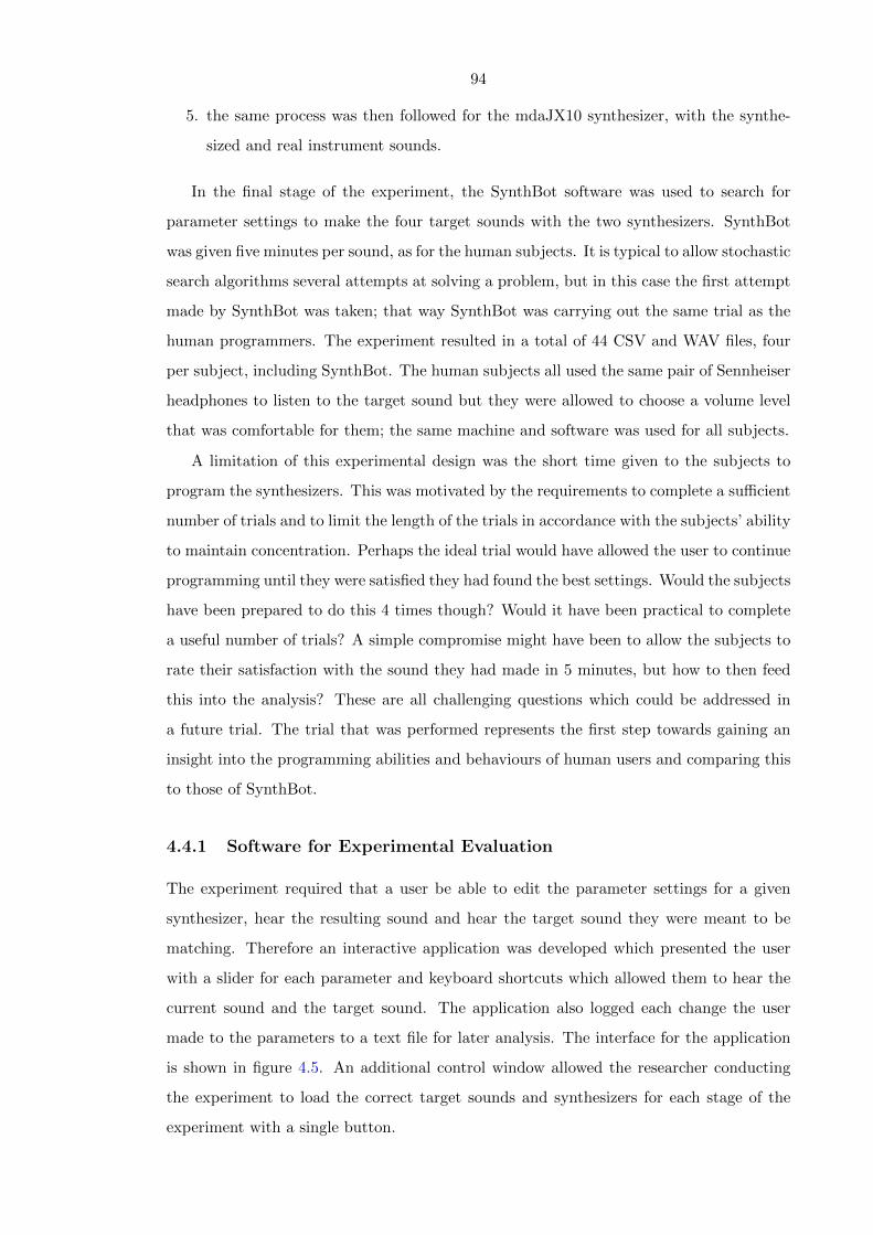
94

5. the same process was then followed for the mdaJX10 synthesizer, with the synthe-

sized and real instrument sounds.

In the final stage of the experiment, the SynthBot software was used to search for

parameter settings to make the four target sounds with the two synthesizers. SynthBot

was given five minutes per sound, as for the human subjects. It is typical to allow stochastic

search algorithms several attempts at solving a problem, but in this case the first attempt

made by SynthBot was taken; that way SynthBot was carrying out the same trial as the

human programmers. The experiment resulted in a total of 44 CSV and WAV files, four

per subject, including SynthBot. The human subjects all used the same pair of Sennheiser

headphones to listen to the target sound but they were allowed to choose a volume level

that was comfortable for them; the same machine and software was used for all subjects.

A limitation of this experimental design was the short time given to the subjects to

program the synthesizers. This was motivated by the requirements to complete a sufficient

number of trials and to limit the length of the trials in accordance with the subjects’ ability

to maintain concentration. Perhaps the ideal trial would have allowed the user to continue

programming until they were satisfied they had found the best settings. Would the subjects

have been prepared to do this 4 times though? Would it have been practical to complete

a useful number of trials? A simple compromise might have been to allow the subjects to

rate their satisfaction with the sound they had made in 5 minutes, but how to then feed

this into the analysis? These are all challenging questions which could be addressed in

a future trial. The trial that was performed represents the first step towards gaining an

insight into the programming abilities and behaviours of human users and comparing this

to those of SynthBot.

4.4.1 Software for Experimental Evaluation

The experiment required that a user be able to edit the parameter settings for a given

synthesizer, hear the resulting sound and hear the target sound they were meant to be

matching. Therefore an interactive application was developed which presented the user

with a slider for each parameter and keyboard shortcuts which allowed them to hear the

current sound and the target sound. The application also logged each change the user

made to the parameters to a text file for later analysis. The interface for the application

is shown in figure 4.5. An additional control window allowed the researcher conducting

the experiment to load the correct target sounds and synthesizers for each stage of the

experiment with a single button.

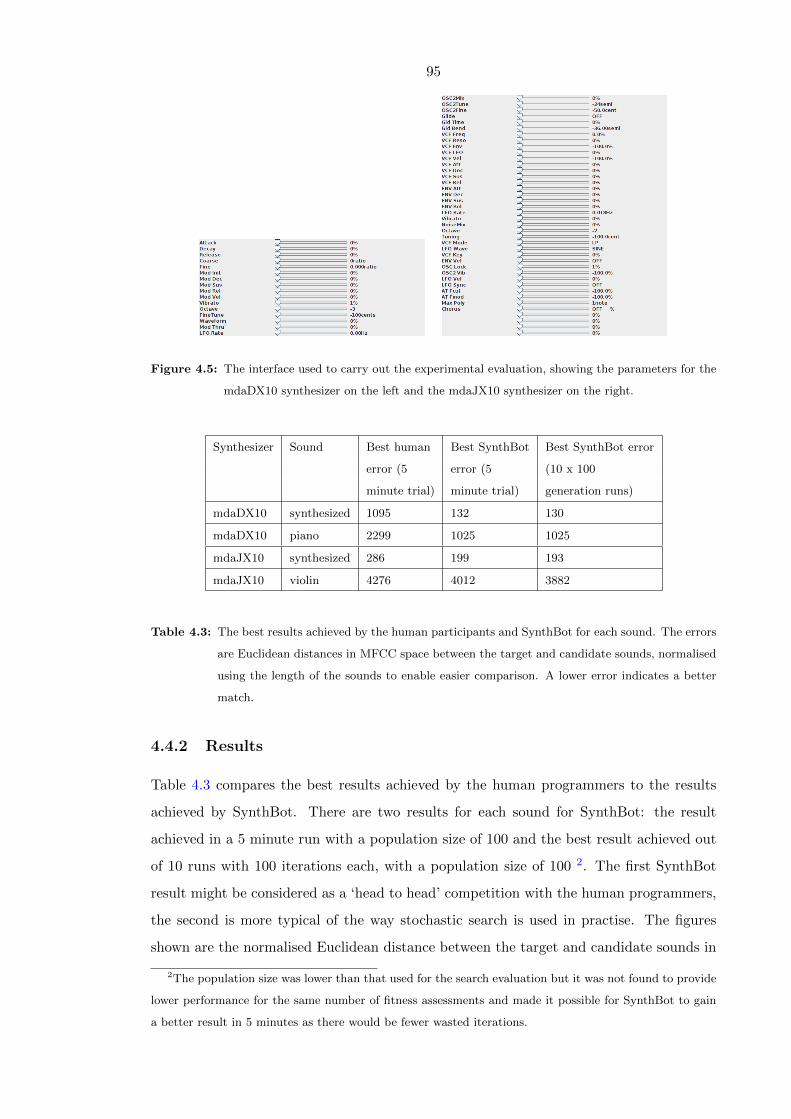
95

Figure 4.5: The interface used to carry out the experimental evaluation, showing the parameters for the

mdaDX10 synthesizer on the left and the mdaJX10 synthesizer on the right.

Synthesizer Sound Best human Best SynthBot Best SynthBot error

error (5 error (5 (10 x 100

minute trial) minute trial) generation runs)

mdaDX10 synthesized 1095 132 130

mdaDX10 piano 2299 1025 1025

mdaJX10 synthesized 286 199 193

mdaJX10 violin 4276 4012 3882

Table 4.3: The best results achieved by the human participants and SynthBot for each sound. The errors

are Euclidean distances in MFCC space between the target and candidate sounds, normalised

using the length of the sounds to enable easier comparison. A lower error indicates a better

match.

4.4.2 Results

Table 4.3 compares the best results achieved by the human programmers to the results

achieved by SynthBot. There are two results for each sound for SynthBot: the result

achieved in a 5 minute run with a population size of 100 and the best result achieved out

of 10 runs with 100 iterations each, with a population size of 100 2. The first SynthBot

result might be considered as a ‘head to head’ competition with the human programmers,

the second is more typical of the way stochastic search is used in practise. The figures

shown are the normalised Euclidean distance between the target and candidate sounds in

2The population size was lower than that used for the search evaluation but it was not found to provide

lower performance for the same number of fitness assessments and made it possible for SynthBot to gain

a better result in 5 minutes as there would be fewer wasted iterations.

96

MFCC space, where the normalisation factors out the length of the sounds. The use of

the same metric for this assessment as the metric used in SynthBot’s genetic algorithm

3 is considered valid, supported by the assertion of the MFCC as a measure of timbral

similarity provided in section 2.4. Further consideration of the validity of this measure is

provided in section 4.5.

In the head to head trials, SynthBot beat the human programmers in every case. The

margin is quite large in all cases except for the mdaJX10 violin sound trial, where the

human programmer nearly matched the SynthBot sound in terms of error; indeed, the

margins for both mdaJX10 sounds were smaller than for the mdaDX10 sounds. There

are different angles to take when explaining this: why was SynthBot relatively better

at programming the mdaDX10 than the mdaJX10 and what in general was causing the

higher errors for the mdaJX10? Referring to the earlier discussion pertaining to the

difficulty of programming FM synthesizers (4.1.1), an explanation for the worse human

FM synthesizer programming could be the non-linearity and unfamiliarity of the controls

compared to the more familiar subtractive synthesis controls found on the mdaJX10. An

explanation for the overall worse performance at mdaJX10 programming could be the

larger number of parameters and presumed increased complexity that follows this. What

is surprising about the mdaJX10 performance is that the humans were able to get so

close to the SynthBot results, even though they were only given 5 minutes to learn the

synthesizer. An explanation for this could be that the average technical musician has had

more experience programming subtractive synthesizers than FM synthesizers, as evidenced

by the prevalence of those types of sounds in electronic music (e.g. tracks using the TB303,

SH101, Moog etc.). Another explanation might be that the ‘search’ approach taken by

human programmers lends itself more to subtractive synthesis. This point is discussed

further in subsection 4.4.2 where human and SynthBot’s parametric trajectories during

search are compared. The resulting sounds can be heard on the accompanying CD, as well

as the author’s website, appendix A, [141].

Spectral Comparison

In figure 4.6, the best results of the first synthesizer programming task, which was to

match a synthesized percussion sound using the mdaDX10, are shown in the form of

spectrograms. As noted in the technical evaluation in section 4.3, this representation is

chosen in preference to an MFCC plot due to its presumed familiarity to the reader. The

3The reciprocal of the non-normalised error is used in the fitness function of SynthBot to assign fitness

to genomes.

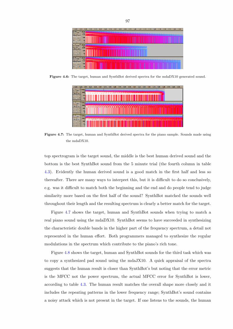
97

Figure 4.6: The target, human and SynthBot derived spectra for the mdaDX10 generated sound.

Figure 4.7: The target, human and SynthBot derived spectra for the piano sample. Sounds made using

the mdaDX10.

top spectrogram is the target sound, the middle is the best human derived sound and the

bottom is the best SynthBot sound from the 5 minute trial (the fourth column in table

4.3). Evidently the human derived sound is a good match in the first half and less so

thereafter. There are many ways to interpret this, but it is difficult to do so conclusively,

e.g. was it difficult to match both the beginning and the end and do people tend to judge

similarity more based on the first half of the sound? SynthBot matched the sounds well

throughout their length and the resulting spectrum is clearly a better match for the target.

Figure 4.7 shows the target, human and SynthBot sounds when trying to match a

real piano sound using the mdaDX10. SynthBot seems to have succeeded in synthesizing

the characteristic double bands in the higher part of the frequency spectrum, a detail not

represented in the human effort. Both programmers managed to synthesize the regular

modulations in the spectrum which contribute to the piano’s rich tone.

Figure 4.8 shows the target, human and SynthBot sounds for the third task which was

to copy a synthesized pad sound using the mdaJX10. A quick appraisal of the spectra

suggests that the human result is closer than SynthBot’s but noting that the error metric

is the MFCC not the power spectrum, the actual MFCC error for SynthBot is lower,

according to table 4.3. The human result matches the overall shape more closely and it

includes the repeating patterns in the lower frequency range; SynthBot’s sound contains

a noisy attack which is not present in the target. If one listens to the sounds, the human

98

Figure 4.8: The target, human and SynthBot derived spectra for the mdaJX10 sound.

Figure 4.9: The target, human and SynthBot derived spectra for the violin sound. Sounds made using

the mdaJX10.

result is a semitone too low yet still a reasonable match, but the SynthBot sound does

seem a better match, especially in the lower frequencies. Since this synthesizer is more

complex, it can be expected that a stochastic search algorithm will not always achieve a

good result. If we consider the best sound generated in ten runs (the final column in table

4.3), the reduction in error is not that great. However, the resulting sound does sound

much closer to the target than the single run result.

Figure 4.9 compares the closest results for the task of synthesizing a violin sound

using the mdaJX10, where SynthBot only achieved a slight improvement over the human

programmers. The spectra of the two results are very different and indeed, they sound very

different. To the author’s ears, the SynthBot sound seems to have more of the roughness

of the violin, but it also has two distinct tones.

Parameter Comparison

Figure 4.10 compares the parameter settings obtained by the human programmers and

SynthBot for the two mdaDX10 programming tasks. The parameter numbers relate to the

parameters shown in table 4.1. In the left hand panel, the actual parameter settings used

to generate the target sound are shown as well as those settings found by the programmers.

There is a greater correlation between SynthBot’s settings and the target than between the

human settings and the target, e.g. parameters 4, 5 and 6 were ignored by the best human

99

0

0.2

0.4

0.6

0.8

1

1.2

0 1 2 3 4 5 6 7 8 9 10 11 12 13 14 15

Para

mete

r valu

e

Parameter number

Synthbot and human derived parameter comparison for mdaDX10 derived sound

targethuman

synthbot

0

0.2

0.4

0.6

0.8

1

1.2

0 1 2 3 4 5 6 7 8 9 10 11 12 13 14 15

Para

mete

r valu

e

Parameter number

Synthbot and human derived parameter comparison for piano sample

humansynthbot

Figure 4.10: Target vs human vs SynthBot derived parameters for the mdaDX10 derived sound on the

left and the piano sample on the right.

0

0.2

0.4

0.6

0.8

1

1.2

0 1 2 3 4 5 6 7 8 9 10 11 12 13 14 15 16 17 18 19 20 21 22 23 24 25 26 27 28 29 30 31 32 33 34 35 36 37 38 39

Para

mete

r valu

e

Parameter number

Synthbot and human derived parameter comparison for mdaJX10 derived sound

targethuman

synthbot

0

0.2

0.4

0.6

0.8

1

1.2

0 1 2 3 4 5 6 7 8 9 10 11 12 13 14 15 16 17 18 19 20 21 22 23 24 25 26 27 28 29 30 31 32 33 34 35 36 37 38 39

Para

mete

r valu

e

Parameter number

Synthbot and human derived parameter comparison for violin sample

humansynthbot

Figure 4.11: Target vs human vs SynthBot derived parameters for the mdaJX10 derived sound on the

left and the violin sample on the right. Note that the sounds were limited to a length of 2

seconds to allow SynthBot to carry out enough iterations in the five minutes allowed. The

parameter indexes can be related back to those shown in 4.1

programmer. The core of the FM synthesis programming takes place in parameters 3-9

which configure the modulator envelope, frequency, index and so on. There is significant

variation between all three sets here, so if one assumes that the sounds are similar (and

listening to them confirms this) then the synthesizer must be quite redundant; there are

several ways to make similar sounds. As for the piano sound, shown in the right panel, the

two programmers do appear to agree on several parameter settings. The volume envelopes

and synthesis parameters are quite similar.

In figure 4.11, the parameters obtained by the best human and SynthBot are shown,

again with the actual parameters for the synthesized target sound in the left panel. There

appears to be very little correlation between the parameter settings here. The violin sound

results in the right panel are completely different.

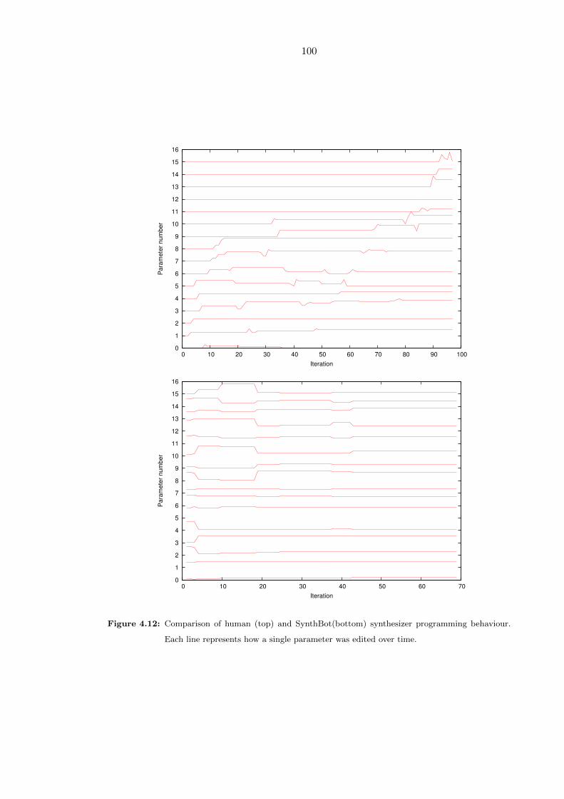
100

0

1

2

3

4

5

6

7

8

9

10

11

12

13

14

15

16

0 10 20 30 40 50 60 70 80 90 100

Para

mete

r num

ber

Iteration

0

1

2

3

4

5

6

7

8

9

10

11

12

13

14

15

16

0 10 20 30 40 50 60 70

Para

mete

r num

ber

Iteration

Figure 4.12: Comparison of human (top) and SynthBot(bottom) synthesizer programming behaviour.

Each line represents how a single parameter was edited over time.

101

Search Behaviour Comparison

In figure 4.12, the programming behaviour of a human and SynthBot when attempting

to copy the mdaDX10 derived sound are compared. The figure shows the edits that

each programmer made to the parameter settings, chronologically. Each horizontal line

represents a different parameter. The data for the SynthBot session was generated by

taking the fittest genome from each iteration of the genetic algorithm and plotting its

values; the data for the human session was generated by taking a snapshot of the parameter

settings every time the user made an edit to any parameter. The programmers behaved

in very different ways: SynthBot adjusts many parameters simultaneously; the human

only adjusts a single parameter at a time; the human continued making large changes to

parameters throughout their session; SynthBot began by making large edits then switched

to small increments, with occasional large jumps; the human parametric explorations

tended to have similar trajectories, where the value was increased gradually from zero to a

high value. It should be noted that the interface being used by the human only allowed the

editing of a single parameter at a time but that it was easy to jump between parameters.

4.5 Conclusion

The problem of programming commercially available synthesizers has been described and

the current state of commercial synthesizer programming interfaces has been briefly dis-

cussed. In summary, synthesizers are hard to program and their manufacturers have

recognised this through the introduction of category based interfaces. Some previous ap-

plications of machine learning to the problem of synthesizer programming have been cited,

including those available for commercial synthesizers such as the Nord Modular G2. The

motivation for the construction of SynthBot, essentially that it did not previously exist

and that it would be useful, has been proffered. It has been shown that it is possible

to construct an automatic, general purpose synthesizer programmer and that by leverag-

ing VST technology, it is possible to integrate the system with industry standard DAW

software. This makes it possible to automatically program a wide variety of synthesizers

with no further work required. The system has been evaluated technically, by assessing its

ability to search the space of possible sounds for a reasonably complex synthesizer. The

result was that SynthBot searched the space effectively for randomly chosen targets in

most cases. The system has been evaluated experimentally by comparing its performance

to that of experienced human synthesizer programmers. The overall result was that Syn-

102

thBot consistently outperforms human programmers in all cases, according to an error

metric based on distance in MFCC feature space. This result could be reinforced through

the use of a human listener study similar to those described in subsection 2.2.4, where

subjects listen to pairs of sounds and rate their similarity. Issues to be addressed by such

a study would include:

1. How should the subjects rate the similarity of sounds? Halpern et al used a fairly

low level method where the subjects rated sounds from high to low similarity using

a 5 button response pad [43]. More elaborate would be a slider with many more

grades of similarity.

2. How to ensure the subjects listen to the sounds in a similar way. In the programming

experiment described in this chapter, the same laptop and headphones were used for

all trials but how to control this in a larger scale, online trial?

Such a study was considered and prototypical software was developed which would

allow the study to be run online but it is left for future work. It would be the first phase

of any further comparison of human and machine synthesizer programming.

In conclusion, a variety of comparisons have been presented in order to detail the

nature of SynthBot’s and human synthesizer programmers’ programming techniques.

4.5.1 Epilogue: The Current State of SynthBot

The latest version of the JVstHost component of SynthBot, which is a Java VST host, is

available from the source code repository website Github wherein significant subsequent

development work has been carried out, mostly by Martin Roth [103]. It currently has

17 registered users following it and 5 developers. The genetic algorithm component has

undergone several iterations since the work described here. The most recent implemen-

tation was a web based service where users could upload an audio file, select a plug-in

and they would then be emailed a preset for that plug-in that made something like their

sound. This system was developed in equal parts by the author and Martin Roth and is

intended to become a commercial product so is not presented in this thesis. The system

was implemented using the Google AppEngine for the HTTP side and a broadly similar

parametric optimisation process to that described in this chapter [20].

In the next chapter, a slightly different application of automatic synthesizer program-

ming is introduced: a self re-programming drum machine.

103

Chapter 5

Sound Synthesis Space

Exploration in Live Performance:

The Evolving Drum Machine

5.1 Introduction

The underlying mechanisms used to produce percussion sound timbres cannot typically be

changed. Acoustic percussion instruments can generally produce a limited set of timbres

with varying loudness but apart from retuning, the instrument’s timbral output cannot

easily be stretched beyond this palette during a performance. Even the snare drum, the

cornerstone of jazz drumming, with its huge variety of timbres cannot change its shape

or material during a performance. In ‘popular’ forms of electronic music such as house

and techno music, the situation is more extreme. The vast majority of drum tracks

for this music are constructed either using classic analogue drum machines such as the

Roland TR909 or using samples of such drum machines (or other drum samples). This

seems at odds with the electroacoustic and experimental strains of electronic music, where

timbral richness and dynamics play a key role. Modern, live performance orientated drum

machines such as the Electribe series from Korg provide means for editing the drum sounds

‘live’ but generally this is limited to ‘tweaking’ the filter cut off or similar transient effects,

it is not feasible to reconfigure the underlying synthesizer live.

The system presented in this chapter attempts to redress the balance by providing its

user with the means for composing rhythmic patterns which are sonified using evolving

percussion synthesizers. A genetic algorithm is used to explore the space of possible

parameter settings for a general purpose, subtractive-style percussion synthesizer modelled

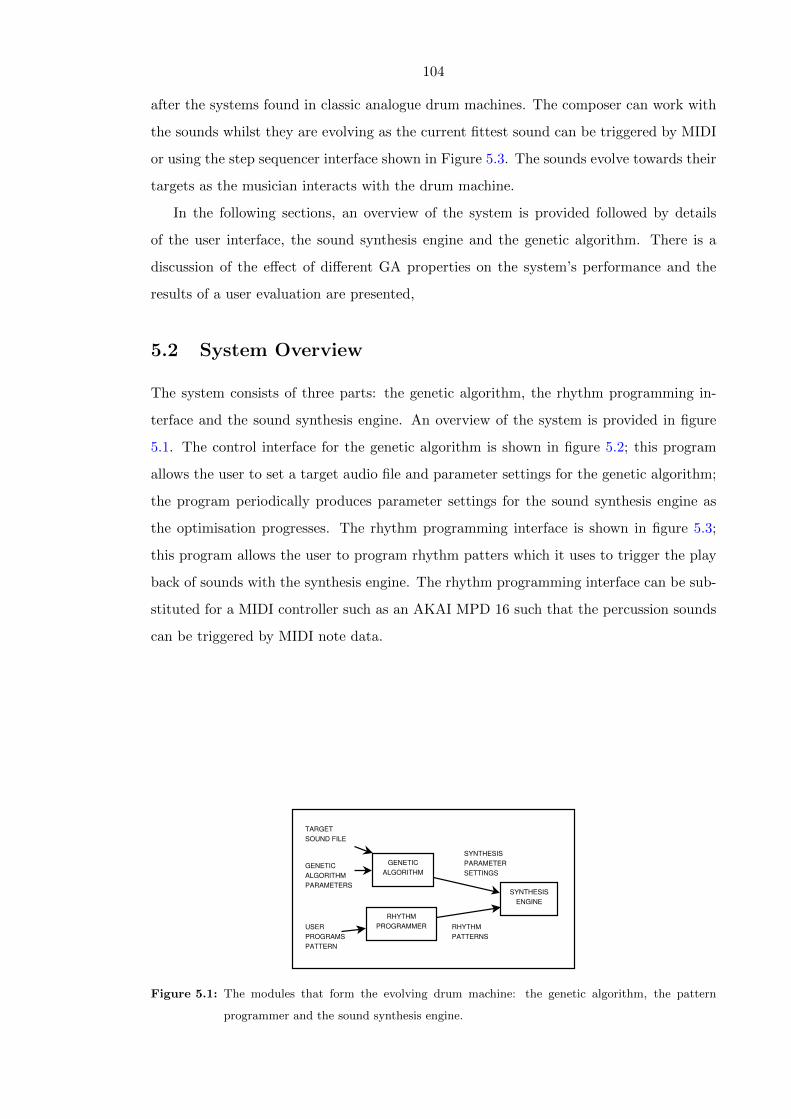
104

after the systems found in classic analogue drum machines. The composer can work with

the sounds whilst they are evolving as the current fittest sound can be triggered by MIDI

or using the step sequencer interface shown in Figure 5.3. The sounds evolve towards their

targets as the musician interacts with the drum machine.

In the following sections, an overview of the system is provided followed by details

of the user interface, the sound synthesis engine and the genetic algorithm. There is a

discussion of the effect of different GA properties on the system’s performance and the

results of a user evaluation are presented,

5.2 System Overview

The system consists of three parts: the genetic algorithm, the rhythm programming in-

terface and the sound synthesis engine. An overview of the system is provided in figure

5.1. The control interface for the genetic algorithm is shown in figure 5.2; this program

allows the user to set a target audio file and parameter settings for the genetic algorithm;

the program periodically produces parameter settings for the sound synthesis engine as

the optimisation progresses. The rhythm programming interface is shown in figure 5.3;

this program allows the user to program rhythm patters which it uses to trigger the play

back of sounds with the synthesis engine. The rhythm programming interface can be sub-

stituted for a MIDI controller such as an AKAI MPD 16 such that the percussion sounds

can be triggered by MIDI note data.

GENETIC

ALGORITHM

RHYTHM

PROGRAMMER

SYNTHESIS

ENGINE

SYNTHESIS

PARAMETER

SETTINGS

RHYTHM

PATTERNS

TARGET

SOUND FILE

GENETIC

ALGORITHM

PARAMETERS

USER

PROGRAMS

PATTERN

Figure 5.1: The modules that form the evolving drum machine: the genetic algorithm, the pattern

programmer and the sound synthesis engine.

105

5.3 User Interface

There are two user interfaces, one that allows the user to specify parameters for the genetic

algorithm and one that allows the user to specify rhythm patterns, shown in figures 5.2 and

5.3, respectively. The parameters the user can specify for the GA are the target sound, the

synthesis engine to use, the population size and the genome mutation mode. Additionally,

the user can stop and start the evolution and listen to or render to disk selected members

of the population. The rhythm programmer is modelled after the typical step sequencer

interfaces found on drum machines such as the Roland TR808; an image of the TR808

interface is provided in figure 5.4 for reference. On the TR808, the buttons along the

bottom of the machine allow the user to switch on or off triggers at that step in the

sequence; the pattern programmer here works in the same way. It also provides volume

controls for each sound and the user can change the tempo with the keyboard. The user

interfaces are implemented in Java and they communicate with the sound synthesis engine

using OpenSoundControl messages [137]. An overview of the software is provided in 5.5.

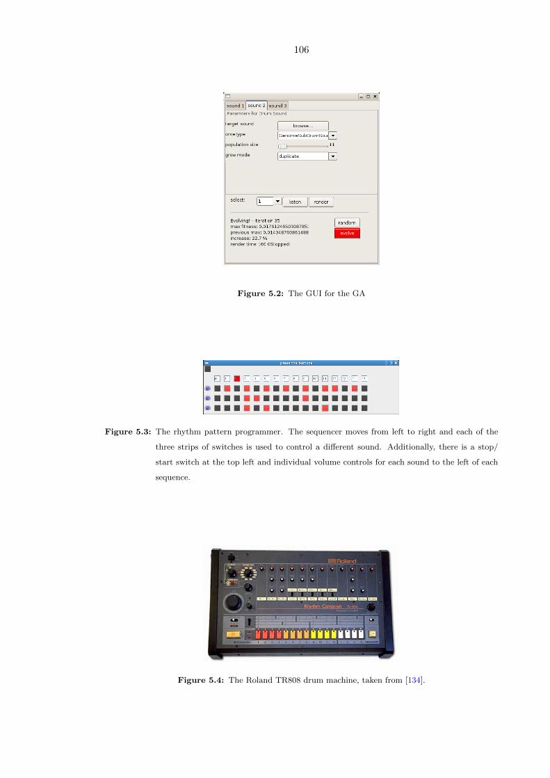
106

Figure 5.2: The GUI for the GA

Figure 5.3: The rhythm pattern programmer. The sequencer moves from left to right and each of the

three strips of switches is used to control a different sound. Additionally, there is a stop/

start switch at the top left and individual volume controls for each sound to the left of each

sequence.

Figure 5.4: The Roland TR808 drum machine, taken from [134].

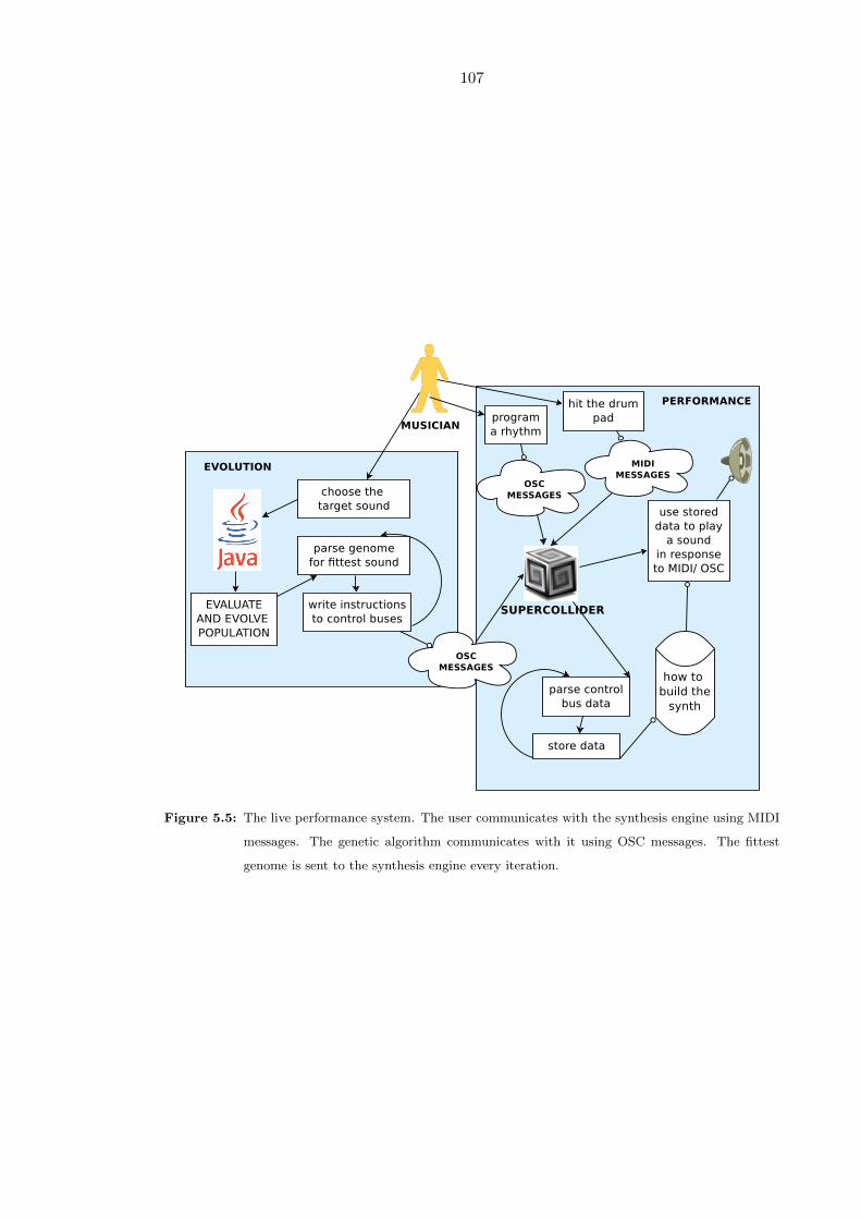
107

Figure 5.5: The live performance system. The user communicates with the synthesis engine using MIDI

messages. The genetic algorithm communicates with it using OSC messages. The fittest

genome is sent to the synthesis engine every iteration.

108

5.4 Sound Synthesis

In this section, some details will be provided about the system used to implement the sound

synthesis module as well as the synthesis algorithms themselves. The sound synthesis

module has been built around the open source SuperCollider software which provides two

main components, sclang and scsynth [77]. Sclang is an object orientated, interpreted

scripting language specialised for music composition and sound synthesis applications.

Scsynth is a real time sound synthesis server which is controlled using Open Sound Control

(OSC) messages sent via a network port [137]. It can also process lists of OSC messages

stored in a file in an offline mode, rendering the output to disk as an audio file. Sounds

in SuperCollider are made using synths. The structure of a synth is defined using a

SynthDef, which is equivalent to a patch in a typical synthesiser or indeed, a class in an

object orientated programming language. SynthDefs define which unit generators (from

the many available in SuperCollider) are to be used in the patch and also arguments that

can be used to change the state of the unit generators in the patch once it is running, e.g.

change the pitch of an oscillator. Once a SynthDef has been registered, by sending it to

scsynth using OSC, it is possible to request that scsynth instantiates this synthdef so that

the audio it generates can be heard, using OSC. The parameters of the synth can be set

at the time of creation and they can be changed later by sending more OSC messages.

As such, a typical use case for SuperCollider would be to define a set of SynthDefs using

sclang then to construct a control program which instantiates and adjusts synths, again

in sclang.

Since OSC is an open network protocol, like HTTP for example, a custom client can

be written to control scsynth, taking over the role of sclang. The client simply needs to

send the correct OSC messages, for real time operation or to write the OSC command file

in the correct format, for non-real time operation. The search component of the system

described in section 5.5 is written in Java and it uses scynth in its offline mode to render

the output of the evolving sounds to disk for fitness analysis. Writing the genetic algorithm

in Java allowed it to be prototyped more rapidly and made it possible to exploit multi-core

CPUs.

The aim was to construct a synthesis engine that would be capable of synthesizing a

variety of percussion sounds in the style of classic analog drum machines. The reader is

referred to the manual of the Waldorf Attack synthesizer for a description of some classic

drum machines’ synthesis algorithms and for more general percussion sound synthesis

information, to the Sound on Sound ‘Synth Secrets’ series [128, 101]. Typical examples

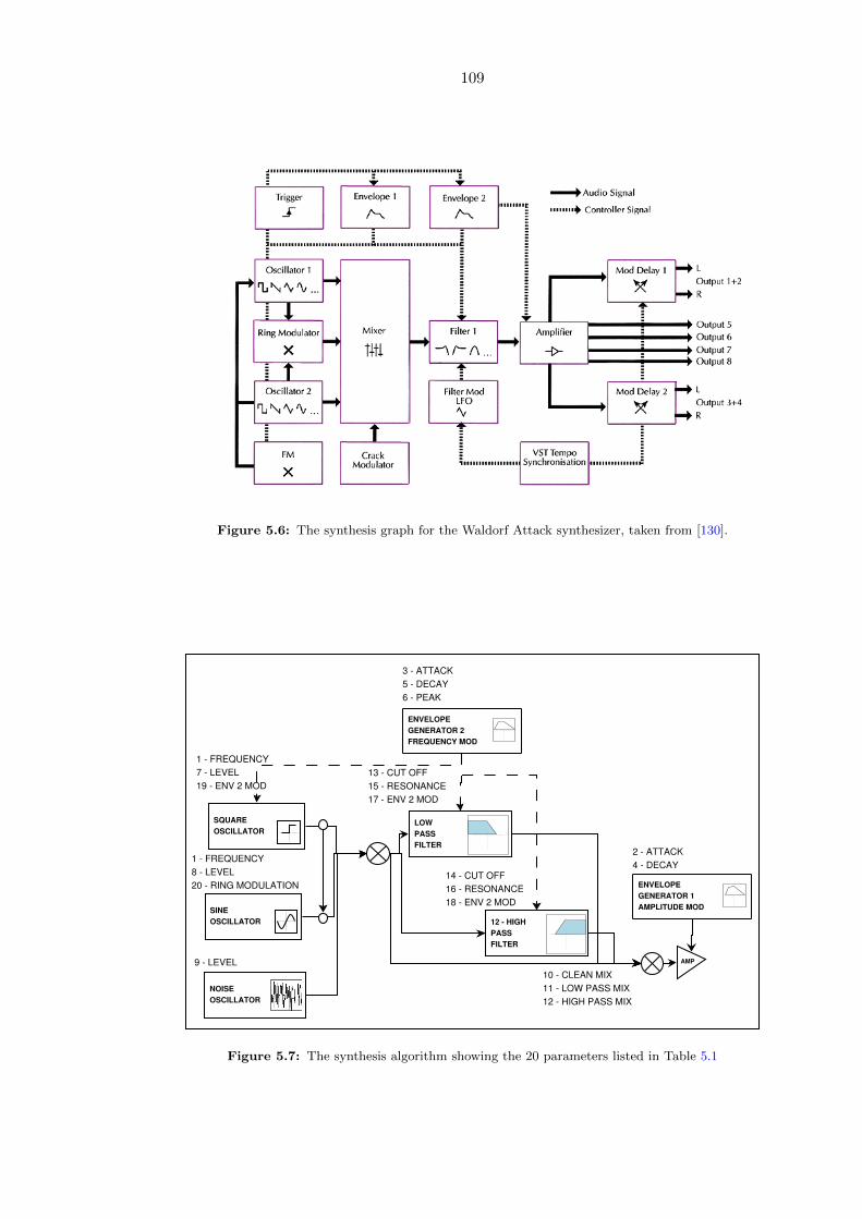
109

Figure 5.6: The synthesis graph for the Waldorf Attack synthesizer, taken from [130].

ENVELOPE

GENERATOR 1

AMPLITUDE MOD

ENVELOPE

GENERATOR 2

FREQUENCY MOD

AMP

13 - CUT OFF

15 - RESONANCE

17 - ENV 2 MOD

14 - CUT OFF

16 - RESONANCE

18 - ENV 2 MOD

1 - FREQUENCY

7 - LEVEL

19 - ENV 2 MOD

SQUARE

OSCILLATOR

LOW

PASS

FILTER

12 - HIGH

PASS

FILTER

3 - ATTACK

5 - DECAY

6 - PEAK

1 - FREQUENCY

8 - LEVEL

20 - RING MODULATION

SINE

OSCILLATOR

NOISE

OSCILLATOR

9 - LEVEL

10 - CLEAN MIX

11 - LOW PASS MIX

12 - HIGH PASS MIX

2 - ATTACK

4 - DECAY

Figure 5.7: The synthesis algorithm showing the 20 parameters listed in Table 5.1

110

are the combination of a high pass filtered noise source and a pure tone to make a snare

drum sound or an impulse plus pitch modulated tone to make a bass drum sound. What

is the motivation for using such a synthesis model as opposed to something more advanced

or esoteric? To explore a well known drum sound aesthetic which is prevalent in much

electronic music and held in high regard will immediately provoke contrasting reactions in

electronic musicians. Further, demands are then made of the system to not just provide

‘interesting’ or ‘esoteric’ sounds, but to provide convincing sounds of a particular character.

The aforementioned Waldorf Attack synthesizer is a virtual analog percussion synthe-

sizer and the synthesis engine used here was largely based on it. The original Attack

synthesis graph is shown in figure 5.6 and the synthesis graph used here is shown in

Figure 5.7. It is controlled via 20 parameters which are listed in table 5.1. A typical

subtractive synthesis model is followed, with a rich source being passed through filters

with modulation on various parameters. There are 3 source oscillators with individual

volume controls providing square, sine and noise waveforms combined with high and low

pass resonant filters arranged in parallel. A modulation envelope provides frequency mod-

ulation for the pitched oscillators and cut off modulation for the high and low pass filters.

Ring modulation occurs between the square and sine oscillators. Finally, an amplitude

envelope controls the level of the overall sound. Once the general form and the parameters

for the synthesis graph were decided, the ranges for the parameters were fine tuned by

ear, by listening to sounds generated with random settings and adjusting the ranges until

an acceptable variety of percussion sounds was heard. The synthesis engine (supported

by the genetic encoding described in subsection 5.5.1) allows sounds to be made using

multiple instances of the synthesis graph running simultaneously.

5.4.1 SoundExplorer Map of Sound Synthesis Space

Figure 5.8 shows a map of timbre space generated using the SoundExplorer tool introduced

in chapter 2. 5 sample sets were transformed into 42 dimensional MFCC space then

multidimensional scaling was used to place the vectors into a 2 dimensional space for

plotting. (More details can be found in section 2.5). 4 of the sample sets were from 4

popular analog 1 Roland drum machines, the TR606, TR707, TR808 and TR909. The

final set consisted of 1000 sounds generated using the drum synthesizer with parameter

settings sampled uniformly at random across their ranges. This image indicates that there

is a reasonable amount of crossover between the timbre spaces of the drum machines and

1The TR909 combined samples and analog sounds [119]

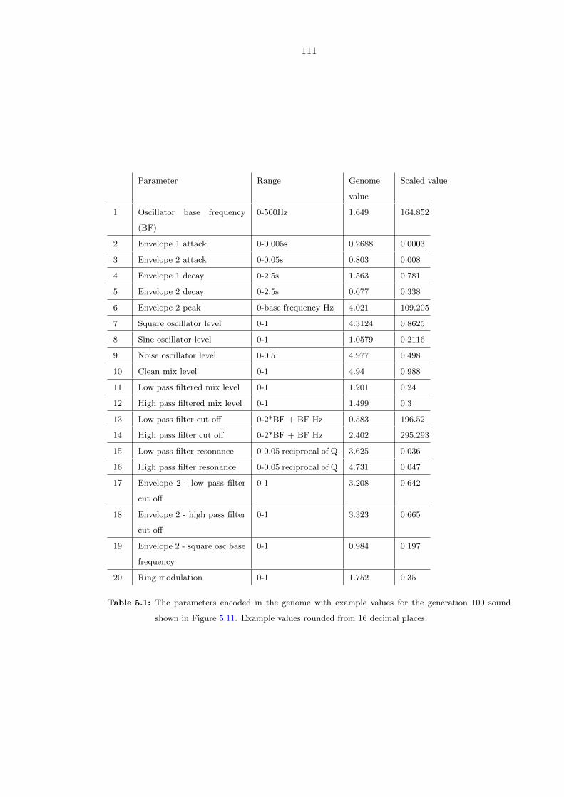
111

Parameter Range Genome

value

Scaled value

1 Oscillator base frequency

(BF)

0-500Hz 1.649 164.852

2 Envelope 1 attack 0-0.005s 0.2688 0.0003

3 Envelope 2 attack 0-0.05s 0.803 0.008

4 Envelope 1 decay 0-2.5s 1.563 0.781

5 Envelope 2 decay 0-2.5s 0.677 0.338

6 Envelope 2 peak 0-base frequency Hz 4.021 109.205

7 Square oscillator level 0-1 4.3124 0.8625

8 Sine oscillator level 0-1 1.0579 0.2116

9 Noise oscillator level 0-0.5 4.977 0.498

10 Clean mix level 0-1 4.94 0.988

11 Low pass filtered mix level 0-1 1.201 0.24

12 High pass filtered mix level 0-1 1.499 0.3

13 Low pass filter cut off 0-2*BF + BF Hz 0.583 196.52

14 High pass filter cut off 0-2*BF + BF Hz 2.402 295.293

15 Low pass filter resonance 0-0.05 reciprocal of Q 3.625 0.036

16 High pass filter resonance 0-0.05 reciprocal of Q 4.731 0.047

17 Envelope 2 - low pass filter

cut off

0-1 3.208 0.642

18 Envelope 2 - high pass filter

cut off

0-1 3.323 0.665

19 Envelope 2 - square osc base

frequency

0-1 0.984 0.197

20 Ring modulation 0-1 1.752 0.35

Table 5.1: The parameters encoded in the genome with example values for the generation 100 sound

shown in Figure 5.11. Example values rounded from 16 decimal places.

112

Figure 5.8: A screen shot from the SoundExplorer program. It shows a map of drum machine timbre

space based on samples of the Roland TR606, TR707, TR808 and TR909 drum machines

along with 1000 random sounds from the synthesis graph shown in figure 5.7, the latter being

shown as small dots.

113

the drum synthesizer, as there are several drum machine sounds placed amongst the drum

synthesizer sounds. However, there are many sounds that are quite far from the spread

offered by the synthesizer. Which sounds can the drum synthesizer match with this data

driven approach and which can it not match? Most of the unmatched sounds in the top

right are bass drum sounds, which typically consist of a complex attack combined with a

sustained tone. Matching the sustained part would require most of the synthesis graph

to be deactivated, save for the sine oscillator or a filtered square wave. Matching the

noisy attack would require a different configuration. Since only sounds made using single

instances of the synthesis graph were used, this is an almost impossible sound to match

well; most random settings will have neither short envelopes nor a pure tonal character.

There is a cluster of snare drums and rim shots in the bottom right, which is also not

covered by the synthesizer. The sounds that are situated within the cloud of sounds

generated from the synthesizer include a variety of drum machines playing snare drums

and cymbals. It is interesting to note that these sounds are noise based whereas the others

are more tonal. A possible explanation could be that in most of the randomly sampled

sounds the noise oscillator level was above zero, meaning the majority of sounds were

closer to the noisy drum sounds than they were to the tonal drum sounds. This is not

so much an indicator of the capabilities of the synthesis algorithm as an artifact of the

parameter setting sampling process. The SoundExplorer tool which was used to generate

this image and which enabled this analysis was developed after the initial version of the

drum machine, so improvements to the sound synthesis engine to better match the space

of sounds inhabited by the Roland drum machines are left for future work.

5.5 Search

The search program employs an unsupervised genetic algorithm which searches an initially

20 dimensional space which represents settings for the synthesis algorithm described in

the previous section. In the following subsections the details of the GA are provided.

5.5.1 Genetic Encoding

The genome contains one or more sets of 20 floating point values in the range 0-5. Each set

can be thought of as a gene, encoding the settings for single instance of the synthesis graph.

The values are scaled by the synthesis engine into appropriate ranges. Table 5.1 lists the

parameters along with example values before and after scaling. When a growth operation

occurs an additional gene will be added in which case the sound will be made using 2

114

complete synthesis graphs (see subsection 5.5.4 for details of genomic manipulations). A

single synthesis graph is shown in Figure 5.7.

5.5.2 Fitness Function

In order to assess a population of sounds, they are first rendered to disk as WAV files by

generating a command OSC file and invoking the SuperCollider synthesis engine in non-

real time mode. Then features are extracted from the audio file and the fitness assigned to

a candidate genome is the reciprocal of the sum squared distance between the candidate

and target features. In the first version of the drum machine, the feature was the power

spectrum where several snapshots were taken of the power spectrum at evenly spaced

positions throughout the sound after Horner [48]. This is the system that was used for the

user evaluations reported in section 5.7. Following further investigation of the literature

on timbre perception and analysis, as presented in chapter 2, the MFCC feature was used

in place of the power spectrum. Early versions of the fitness function compared only

the available frames of the candidate sounds, e.g. if the candidate sound contained 100

frames and the target 200, only the first 100 were considered. It was observed that the

population converged on very short sounds, as they effectively ducked the fitness function.

This problem was solved by assuming feature values of zero where there was a length

mismatch.

5.5.3 Breeding Strategies

The system provides different breeding strategies. The most basic uses a single popula-

tion of individuals with a uniform mutation rate where the next generation is made by

crossing over and mutating the two fittest genomes from the previous generation. The

fittest genome is also added to the next generation to provide elitism. A more complex

breeding strategy splits the population into several islands. The genomes from each island

are assessed for fitness independently and the islands can have a varying mutation rate.

Migration can occur from one island to another, where a random individual from one

island is moved to another island; this means the islands can change size.

5.5.4 Genome Manipulation

New genomes are created by crossing over the two fittest genomes then mutating them.

Mutation can occur in different ways, illustrated in figure 5.9:

1. All loci mutation adds or subtracts a constant from all loci in the genome. The size

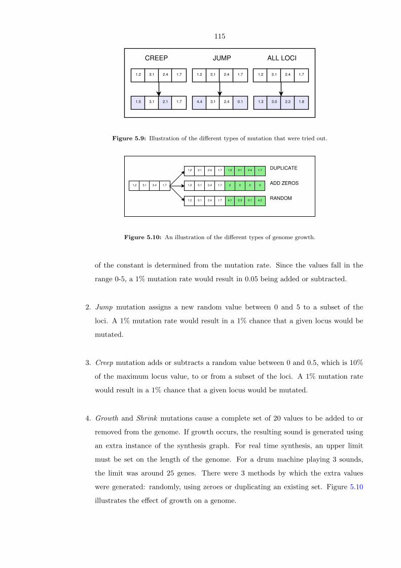
115

1.2 3.1 2.4 1.7

1.3 3.0 2.2 1.8

1.2 3.1 2.4 1.7

4.4 3.1 2.4 0.1

1.2 3.1 2.4 1.7

1.5 3.1 2.1 1.7

CREEP JUMP ALL LOCI

Figure 5.9: Illustration of the different types of mutation that were tried out.

1.2 3.1 2.4 1.7

1.2 3.1 2.4 1.7

1.2 3.1 2.4 1.7 0 0 0 0

4.1 2.3 0.1 4.21.2 3.1 2.4 1.7RANDOM

DUPLICATE

ADD ZEROS

1.2 3.1 2.4 1.7

Figure 5.10: An illustration of the different types of genome growth.

of the constant is determined from the mutation rate. Since the values fall in the

range 0-5, a 1% mutation rate would result in 0.05 being added or subtracted.

2. Jump mutation assigns a new random value between 0 and 5 to a subset of the

loci. A 1% mutation rate would result in a 1% chance that a given locus would be

mutated.

3. Creep mutation adds or subtracts a random value between 0 and 0.5, which is 10%

of the maximum locus value, to or from a subset of the loci. A 1% mutation rate

would result in a 1% chance that a given locus would be mutated.

4. Growth and Shrink mutations cause a complete set of 20 values to be added to or

removed from the genome. If growth occurs, the resulting sound is generated using

an extra instance of the synthesis graph. For real time synthesis, an upper limit

must be set on the length of the genome. For a drum machine playing 3 sounds,

the limit was around 25 genes. There were 3 methods by which the extra values

were generated: randomly, using zeroes or duplicating an existing set. Figure 5.10

illustrates the effect of growth on a genome.

116

Figure 5.11: Example sounds from an evolutionary run, time domain plot at the bottom and frequency

domain plot at the top. The sounds shown are the fittest from generation 1, 50 and 100

then the target sound, a Roland TR808 snare drum.

5.6 Results: GA Performance

5.6.1 General Performance

On a dual core Athlon X2 2.2 GHz system evolving 3 populations simultaneously, the

assessment time per genome was approximately 150ms, which varied depending on the

length of the sound. With 3 populations of 50 genomes to assess, that meant the sounds

heard from the drum machine changed once every 22.5s. On the 1.8 GHz single core

Intel Dothan system employed for user testing, the time increased to around a minute

per change, so the population size was decreased to 20 for the user tests. The effect

of waiting for the sounds to change was lessened since the 3 populations were evolving

asynchronously. A parametric interpolation function was also used, where the synthesizer

linearly interpolated its parameters to their new settings over a period of 10 seconds. This

effect was especially interesting when a new module was added to a growable genome, as

the module’s settings would start at zero and fade to their selected positions. An example

of an interpolated evolutionary run with a sound played at regular intervals can he heard

on the accompanying CD or the author’s website, appendix A, [141].

5.6.2 Algorithm Settings and Their Effect on Musical Output

Whilst part of the focus of this work is an exploration of the artistic applications of genetic

algorithms and the musical results of this, some analysis of the system’s search performance

was essential to indicate future technical directions for the work. Decisions made at the

technical level clearly have an impact on the sound and behaviour of the system. Detailed

technical performance analyses of tone matching systems are available in chapters 3 and

117

section 4.3. Here, there is an observational assessment of the musical behaviours resulting

from different permutations of the GA parameters.

Island Population Model

Whitley argues that the island population model provides increased performance in the

case where the different objectives of a multi-objective optimisation problem are linearly

separable and can thus be solved individually in parallel [133]. Migration then allows the

combination of the individual solutions to provide what is likely to be closer to a global

maximum. The problem of synthesizer design could be described as multi-objective since

the requirement is to generate a series of spectral feature vectors in the correct order

and different parts of the synthesizer can generate different feature vectors at different

times. If one considers the grow mutation, where new components can be added to the

synthesis algorithm, perhaps each island could converge on a good match for a different

aspect of the sound. For example, the classic TR808 kick drum starts with a short click

and continues with a sustained pure tone with slight pitch modulation; one island could

evolve the click, the other the tone and the combination would be a close match. It

is expected that the growth operation will play an important role in increasing linear

separability of the synthesizer programming task, since there are distinct units that can

be evolved somewhat independently. In the absence of growth mutations, the matching

results did not show any performance advantage when using the island model which may

indicate that this particular problem is not linearly separable. It is likely that the linear

separability is reduced by epistatic effects between loci. For example the base frequency

parameter affects envelope 2 and both of the filters. The parameters for envelope 2 have

more complex epistatic effects as it modulates several parts of the synthesizer. Enabling

the growth operator did indeed produce genomes that had separate genes for different parts

of the sound, as observed through careful listening; this is an interesting phenomenon that

warrants a more in depth study.

Different Mutation Types

To assess the effect of the different mutation types, several runs were carried out with pop-

ulation size 50 and different mutation types. Jump mutation provided consistently poor

performance. All loci mutation provided excellent performance for the hi-hat but poor

performance for the snare drum. 10 more runs were carried out to check this observation

and it was observed that all loci mutation provides consistently faster convergence than

118

creep mutation for the hi-hat sound but that the convergence fitness was consistently lower

than the creep mutation runs; this was premature convergence. This suggests that varying

the mutation type across islands as well as mutation rate might increase the performance.

The growth operator had 3 modes of operation: add random values, add zeroes and add

a duplicate. It was observed that adding random values and zeroes typically resulted in

shorter genomes, i.e. the genomes with additional genes were not selected for. When the

duplicate mode was used, the genomes tended to increase in length for some target sounds,

but not for others. For example, the genomes evolved for TR808 kick drums and cow bells

always used as many genes as were allowed whereas snare drums and hats tended to use

only one gene.

So what is the musical result of a genome with or without epistatic effects? What is

the effect of different types and rates of mutation? For the purposes of this discussion

the operation of the evolving drum machine in a live performance context is considered,

where the performer is triggering the sounds using a MIDI drum pad. The first, rather

obvious observation is that the evolving drum sounds move gradually from nondescript

start sounds towards the target sounds. But why do they not make larger jumps? Possibly

since the epistasis in the genome prohibits the cleanly modular evolution possible with a

linearly separable problem. The population size has an impact here as well - a larger

population produces the same rate of increase of fitness but in fewer iterations, so small

populations are preferable to provide musically interesting, frequent and small jumps.

In her work composing with genetic algorithms, Magnus evolves time domain audio

data directly towards a target sound and she explicitly states that the evolutionary op-

timisation process is being used as part of the style of the piece [75]. The target sound

is changed mid evolution and different types of mutation are applied and it is observed

that this adds to the musicality of the piece, varying its dynamics. It was observed with

the evolving drum machine that the initial phase of evolution was more rapid and that

this provided an interesting movement to the musical output. Changing the target sound

automatically and periodically before the fitness increase levelled off kept the system in

a perpetual state of rapid convergence. Changing targets is also a challenge to the per-

former, who must decide which of the available sounds is appropriate for which part of

the rhythm. A low mutation rate can slow the evolution down, offering a more gradual

exploration of the space of possible drum sounds. A high mutation rate provides a series

of much more random sounds, if the elitism which retains the previous fittest genome is

deactivated.

119

5.7 Results: User Experiences

Besides the author’s experience of using the system discussed in the previous section,

initial user testing was carried after the Conceptual Inquiry model which aims to answer

the question:

How can we get detailed information about how people work when they cannot

articulate it on their own? Holtzblatt and Beyer, 1993 [47].

The inquiry is carried out by means of an interactive session with a user, an interviewer

and the system in question. The user attempts to carry out the task for which the system

was designed, a task with which they have familiarity and the interviewer attempts to

gain information about the way the user does this. It is observed that the user finds it

easier and more pertinent to express opinions in this context than in a non-contextual

interview [47]. The Contextual Inquiry model was originally intended to form part of

the process of system design, where the designer collects information about the way users

carry out a particular task and attempts to model a new system on this information. In

the case of this trial, the system had already been designed so it does not fit into this

typical methodology but the theme on inquiry in context holds true. Another approach

would be a questionnaire, but this forfeits the opportunity for impromptu, contextual

discussion. This has proved to be a useful first approach to assessing the evolving drum

machine as the users were able to immediately start composing with the system, then to

learn about and respond to its peculiarities. So far, two musicians have been invited to

compose rhythm patterns with the system whilst asking and answering questions. This is

not sufficient to constitute a full evaluation of the system but it does provide some insight

into the usefulness of artificial life derived music tools for musicians. The MFCC error

metric was not in place when these trials were carried out, as mentioned in subsection

5.5.2 but the sound matching was considered good enough with the power spectrum error

metric for the purposes of these trials, which are less focused on perfect sound matching

and more focused on the overall experience of using a drum machine whose sounds morph

to a target sound over time.

The users were first presented with the sequencer interface shown in Figure 5.3 with

which they interacted whilst the sounds evolved. Some initial questions were asked and

then the underlying evolutionary process was explained. They were then given access to

the search algorithm interface and allowed to continue composing, but this time they could

change settings on the GA such as the target sound file. The musicians interviewed had

120

different backgrounds: musician 1 uses Roland analogue drum machines and synthesizers in

an improvisational context to compose somewhat noisy electronic music and could be seen

as a drum machine virtuoso; musician 2 is a skilled guitar player who composes melodically

sophisticated music using industry standard tools such as Cubase and GigaSampler.

Musician 1 noted that the sounds reminded him of the sounds from early, more primi-

tive drum machines such as the Roland CR78. He also observed that the sounds improved

in quality as the evolution progressed and (once he was informed as to the underlying

process) that they became recognisably similar to the specified target sounds (which were

in this case samples of a Roland TR808). He would be interested in using these drum

sounds in his compositions, wherein the drum sounds are normally sourced from analogue

drum machines, synthesizers and effects units in various configurations. He made the

observation that sometimes the sound that was supposed to be the snare was actually of

more use as a bass drum. This ties in with the GA performance observation that there is

a larger variation in the convergence fitness for the snare drum than for the other sounds

- perhaps the snare drum is more difficult to match due to having the tonal component

of the bass drum along with the noise component of the hi-hat. He stated that the re-

linquishing of control to the machine and the deliberate exploration of the accidental, a

process embodied in such a system, was a valid aesthetic in itself but that in this case

the human does need to maintain editorial control. He suggested various improvements

that could be made to the interface, such as displaying more information about the target

sound.

Musician 2, with their leaning towards a more traditional musical aesthetic found the

evolutionary method of exploration to be a refreshing approach to making drum sounds,

which he normally constructs from samples or simple virtual synthesizer patches. He was

happy to relinquish control of the sound design process to the machine, accepting this as

a valid technique by which unique sounds could be made. Before being told much of the

underlying system, he said he was using pitch and volume dynamics to decide which sound

should be used for which part of the drum kit. If the sound that was evolving towards

a snare sample was pitched lower than the sound evolving towards a bass drum sample,

he would use the snare seeker as a bass drum. As the evolution progressed, he tended to

map the sounds to their appropriate parts. He suggested that the system would be more

useful if the sounds could be triggered from a MIDI sequencer (a later development) and

that volume controls (later added) would be of use.

121

5.8 Conclusion

The implementation of a drum machine with ever-changing timbres has been described

and the effects of variations in the genetic algorithm used to drive the system have been

discussed in a technical and creative context. The results of initial user trials are very pos-

itive, indicating that a successful combination of novelty and appliance has been achieved.

In the following chapter, another application of genetic algorithm driven sound synthesis

is described: an autonomous timbral and melodic improviser.

122

Chapter 6

The Timbre Matching Improviser

The purpose of this chapter is to present the final creative application of sound synthesis

space search: the timbre matching improviser. The system described is an autonomous

musical agent which would be considered as a performance driven, transformative player

according to Rowe’s taxonomy of such systems. The improviser listens through pitch and

timbre detectors and attempts to follow and transform the timbres and note patterns

played by the human player. The chapter provides some background on the previous work

with autonomous musical agents and then describes the technical implementation of this

new system. The 4 parts of the system, namely the genetic algorithm, synthesis engine,

listening component and performance component are described in detail. The musical

behaviour of the system is discussed along with feedback from a musician who has played

alongside it many times. The system has been used in a variety of recording sessions

and live performances and the author’s experience of working in these scenarios with the

system is recounted.

6.1 Related Work

The construction of complete, automated improvisation systems which respond in real time

to the sounds made by human improviser(s) by generating complementary sonic gestures

is a well established activity in computer music research. Rowe introduced a classification

scheme for interactive music systems which covers the gamut from user controlled exten-

sions of traditional instruments through to full autonomous agents [104]. According to

this taxonomy, the system under discussion here is a performance driven, transformative

player. See subsection 1.1 for more details on this taxonomy. A variety of systems have

been described which are capable of improvising alongside human players: Biles’ GenJam

123

is ‘a genetic algorithm-based model of a novice jazz musician learning to improvise’ [8].

Thom’s BoB is an improvisational companion whose ‘central focus is user-specific live

melodic interaction’ where “unsupervised machine learning techniques are used to auto-

matically configure BoB’s aesthetic musical sense to that of its specific user/musician”

[122]. Lewis’ Voyager has been developed over many years and he defines it as a ‘virtual

improvising orchestra’ built around the idea of ‘multidominance’ of several simultaneous

musical streams [71]. Blackwell and Young coin another term for such systems, ‘Live

Algorithms’:

A Live Algorithm takes part in improvised, collaborative performance, sharing

the same modes of communication and expression as its partners. Autonomous

rather than automated or controlled, the device enjoys the same constraints

and freedoms as its human associates. Blackwell and Young 2005 [9].

In a subsequent paper, Young defines several attributes of live algorithms [145]. Adapt-

ability is the ability to adapt to a shared environment; empowerment is essentially decision

making autonomy; intimacy is the notion of a shared nuance and wider characteristics be-

tween man and machine’s musical output; opacity is the avoidance of direct cause and

effect, where interactivity should avoid becoming Lewis’ ‘metonym for information re-

trieval’ and unimagined covers ideas of unknown or unimagined music being produced

[71]. Collins presents a selection of autonomous musical agents and multi-agent systems,

where the shared thread is the use of signal processing based listening techniques for onset

and pitch detection and the associated higher level interpretations of meter and rhythmic

phase [24]. Collins touches on several of Young’s attributes in reporting the feedback from

guitarist Ian Cross, who performed with Collins’ ‘Free Improvisation Simulation’ [24, p.

178-184]. For example, Cross specifically mentions opacity of intent and different levels

of intimacy. The system presented here is evaluated partly in terms of these attributes in

subsection 6.3.2.

6.1.1 Genetic Algorithm Driven Sound Synthesis

In this subsection, the research topic of interactive genetic algorithms is introduced. Pre-

vious sections have dealt with non-interactive genetic algorithms (1.1, 4.1.2) but the im-

proviser is the first system in this thesis which allows the user to specify the target for the

search in a more interactive way than by choosing a WAV file.

Several researchers have used interactive genetic algorithms to allow a user to guide

the evolution of parameters for a sound synthesis algorithm. Such systems allow even

124

a novice ‘sound synthesist’ to explore a complex space of possible parameters to find

unique and dynamic sounds, sounds which they would not otherwise have been able to

design. For example, see Takala et al., Yee-King, Johnson, Collins and McDermott et al

[120, 139, 59, 23, 79]. The systems present their user with a variety of sounds which the

user must rate. The ratings are then fed back to the GA which uses them as if they were

the output of a standard fitness function. The next generation is created and the user

repeats the activity. A limitation of such systems is the user’s inability to audition large

numbers of different sounds which takes too long and can become tedious. Yee-King’s

AudioServe system attempts to solve this problem by pooling the opinions of several users

over time and space using a collaborative, networked, interactive GA [139, 136]. In this

system, a Java applet embedded in a web page presents a user with a population of

sound synthesis algorithms which they can audition and mutate; they can also upload the

algorithms to a database. Algorithms uploaded to the database are then sent to people

using the applet, as an additional population of ‘immigrants’. The user can choose from

their own local population or the immigrant population. Algorithms can go through many

iterations of selection and mutation on different machines across the network. Thus it is

possible to pick up very fit sounds and work with those or to start from scratch. Users

of the system reported a very engaging experience and the database contained a large

number of complex and interesting sounds by the end of the online run.

Another solution is to allow the user to explicitly specify a target sound or timbre and

to use an unsupervised GA to search for a synthesis algorithm which can generate a sound

resembling the target. Such systems are closer to Holland’s classic GA [46]. Previous work

in this area is detailed elsewhere in this thesis, in sections 1.1 and subsection 4.1.2 and

an in-depth study of the performance of GAs at this task compared to other methods of

parametric optimisation is presented in chapter 3.

Part of the work presented here is technically similar to the GA work discussed above

but it also infuses ideas from the areas of interactive music systems and autonomous

musical agents. In a pragmatic discussion of how to generate musically interesting results

using such systems, Bown and Lexer suggest allowing them to interact with an experienced

musician who can guide the algorithm to interesting musical spaces, exploiting the skill of

the musician and the exploratory power of an algorithm [11]. The work presented here is

therefore a fusion of these areas: a live algorithmic improviser which uses an unsupervised,

yet unobtrusively interactive GA to design its sounds, guided timbrally and melodically

by a live musician.

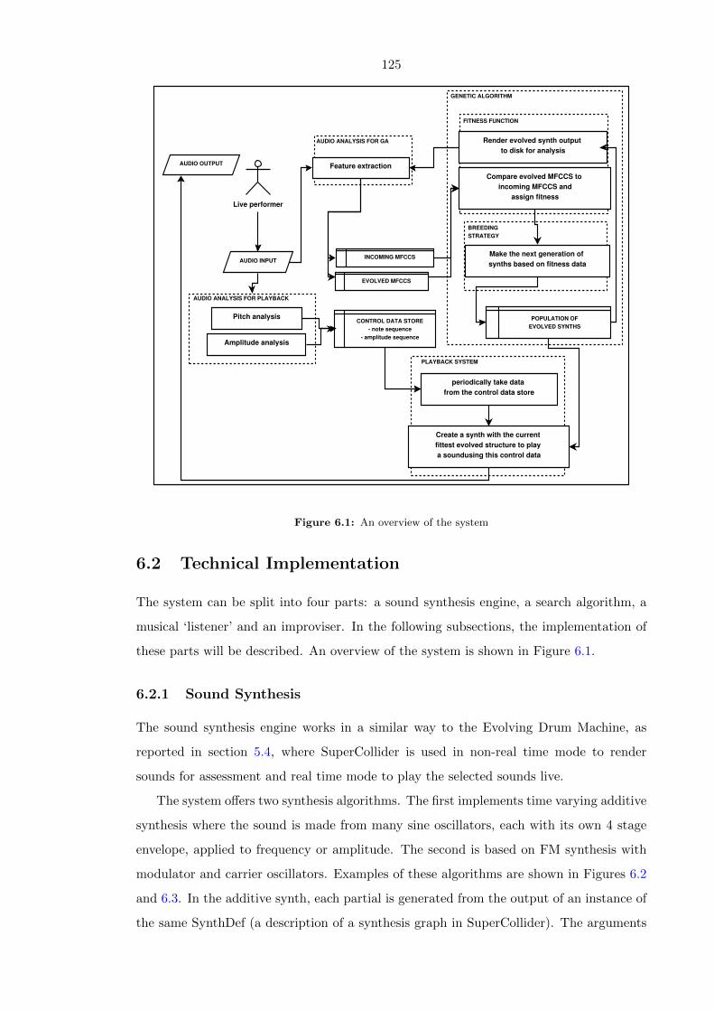
125

AUDIO ANALYSIS FOR GA

Feature extraction

GENETIC ALGORITHM

PLAYBACK SYSTEM

AUDIO INPUT

CONTROL DATA STORE

- note sequence

- amplitude sequence

Live performer

periodically take data

from the control data store

Create a synth with the current

fittest evolved structure to play

a soundusing this control data

AUDIO OUTPUT

FITNESS FUNCTION

Render evolved synth output

to disk for analysis

Compare evolved MFCCS to

incoming MFCCS and

assign fitness

INCOMING MFCCS

EVOLVED MFCCS

BREEDING

STRATEGY

Make the next generation of

synths based on fitness data

POPULATION OF

EVOLVED SYNTHS

AUDIO ANALYSIS FOR PLAYBACK

Pitch analysis

Amplitude analysis

Figure 6.1: An overview of the system

6.2 Technical Implementation

The system can be split into four parts: a sound synthesis engine, a search algorithm, a

musical ‘listener’ and an improviser. In the following subsections, the implementation of

these parts will be described. An overview of the system is shown in Figure 6.1.

6.2.1 Sound Synthesis

The sound synthesis engine works in a similar way to the Evolving Drum Machine, as

reported in section 5.4, where SuperCollider is used in non-real time mode to render

sounds for assessment and real time mode to play the selected sounds live.

The system offers two synthesis algorithms. The first implements time varying additive

synthesis where the sound is made from many sine oscillators, each with its own 4 stage

envelope, applied to frequency or amplitude. The second is based on FM synthesis with

modulator and carrier oscillators. Examples of these algorithms are shown in Figures 6.2

and 6.3. In the additive synth, each partial is generated from the output of an instance of

the same SynthDef (a description of a synthesis graph in SuperCollider). The arguments

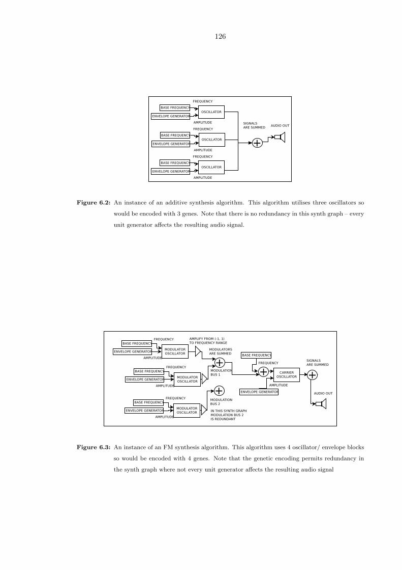
126

Figure 6.2: An instance of an additive synthesis algorithm. This algorithm utilises three oscillators so

would be encoded with 3 genes. Note that there is no redundancy in this synth graph – every

unit generator affects the resulting audio signal.

Figure 6.3: An instance of an FM synthesis algorithm. This algorithm uses 4 oscillator/ envelope blocks

so would be encoded with 4 genes. Note that the genetic encoding permits redundancy in

the synth graph where not every unit generator affects the resulting audio signal

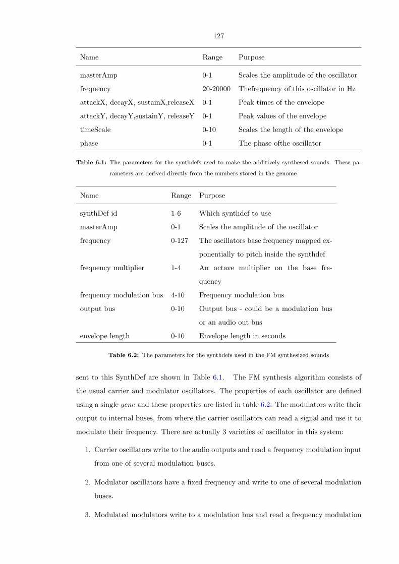
127

Name Range Purpose

masterAmp 0-1 Scales the amplitude of the oscillator

frequency 20-20000 Thefrequency of this oscillator in Hz

attackX, decayX, sustainX,releaseX 0-1 Peak times of the envelope

attackY, decayY,sustainY, releaseY 0-1 Peak values of the envelope

timeScale 0-10 Scales the length of the envelope

phase 0-1 The phase ofthe oscillator

Table 6.1: The parameters for the synthdefs used to make the additively synthesed sounds. These pa-

rameters are derived directly from the numbers stored in the genome

Name Range Purpose

synthDef id 1-6 Which synthdef to use

masterAmp 0-1 Scales the amplitude of the oscillator

frequency 0-127 The oscillators base frequency mapped ex-

ponentially to pitch inside the synthdef

frequency multiplier 1-4 An octave multiplier on the base fre-

quency

frequency modulation bus 4-10 Frequency modulation bus

output bus 0-10 Output bus - could be a modulation bus

or an audio out bus

envelope length 0-10 Envelope length in seconds

Table 6.2: The parameters for the synthdefs used in the FM synthesized sounds

sent to this SynthDef are shown in Table 6.1. The FM synthesis algorithm consists of

the usual carrier and modulator oscillators. The properties of each oscillator are defined

using a single gene and these properties are listed in table 6.2. The modulators write their

output to internal buses, from where the carrier oscillators can read a signal and use it to

modulate their frequency. There are actually 3 varieties of oscillator in this system:

1. Carrier oscillators write to the audio outputs and read a frequency modulation input

from one of several modulation buses.

2. Modulator oscillators have a fixed frequency and write to one of several modulation

buses.

3. Modulated modulators write to a modulation bus and read a frequency modulation

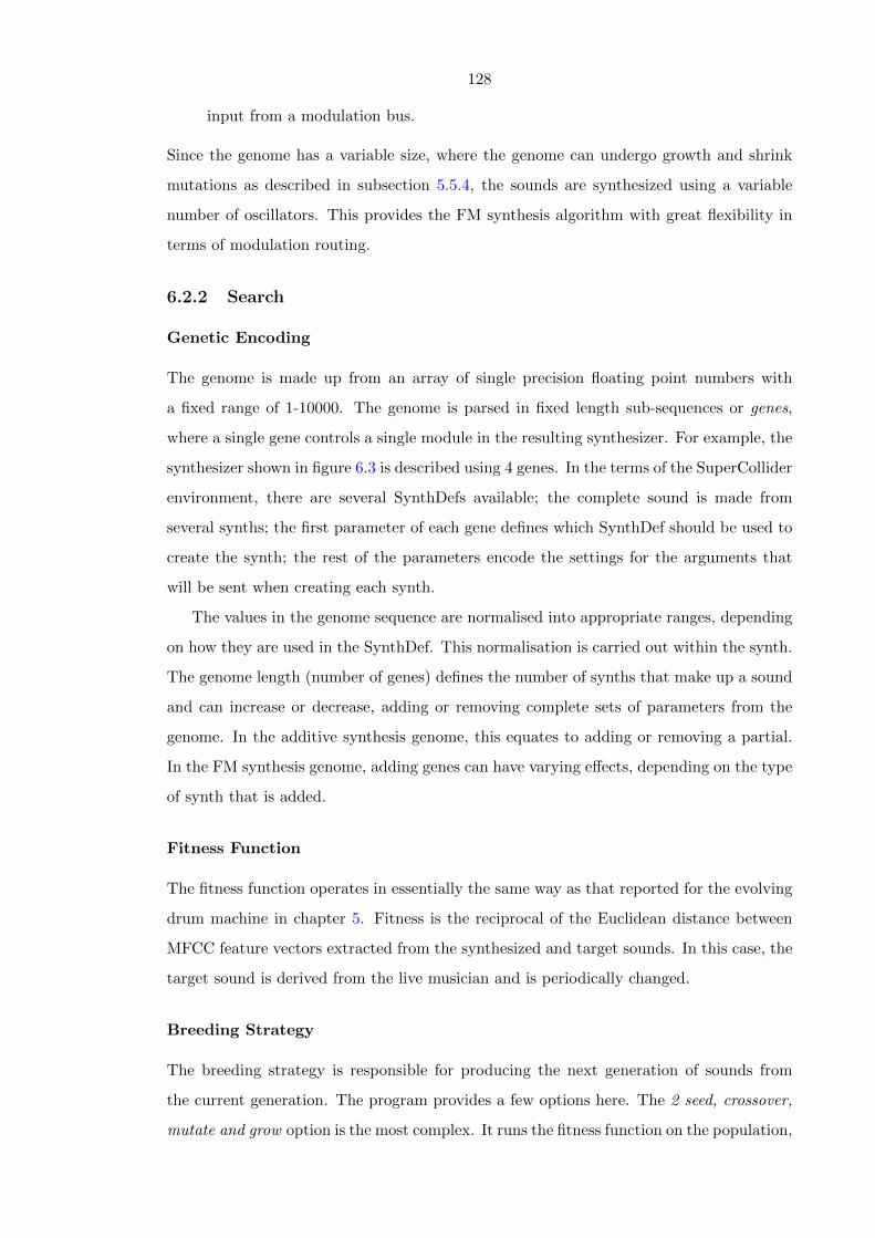
128

input from a modulation bus.

Since the genome has a variable size, where the genome can undergo growth and shrink

mutations as described in subsection 5.5.4, the sounds are synthesized using a variable

number of oscillators. This provides the FM synthesis algorithm with great flexibility in

terms of modulation routing.

6.2.2 Search

Genetic Encoding

The genome is made up from an array of single precision floating point numbers with

a fixed range of 1-10000. The genome is parsed in fixed length sub-sequences or genes,

where a single gene controls a single module in the resulting synthesizer. For example, the

synthesizer shown in figure 6.3 is described using 4 genes. In the terms of the SuperCollider

environment, there are several SynthDefs available; the complete sound is made from

several synths; the first parameter of each gene defines which SynthDef should be used to

create the synth; the rest of the parameters encode the settings for the arguments that

will be sent when creating each synth.

The values in the genome sequence are normalised into appropriate ranges, depending

on how they are used in the SynthDef. This normalisation is carried out within the synth.

The genome length (number of genes) defines the number of synths that make up a sound

and can increase or decrease, adding or removing complete sets of parameters from the

genome. In the additive synthesis genome, this equates to adding or removing a partial.

In the FM synthesis genome, adding genes can have varying effects, depending on the type

of synth that is added.

Fitness Function

The fitness function operates in essentially the same way as that reported for the evolving

drum machine in chapter 5. Fitness is the reciprocal of the Euclidean distance between

MFCC feature vectors extracted from the synthesized and target sounds. In this case, the

target sound is derived from the live musician and is periodically changed.

Breeding Strategy

The breeding strategy is responsible for producing the next generation of sounds from

the current generation. The program provides a few options here. The 2 seed, crossover,

mutate and grow option is the most complex. It runs the fitness function on the population,

129

chooses the two fittest sounds then generates a population of new genomes by crossing

over, mutating and growing the fittest genomes. The growing function, described in more

detail in subsection 5.5.4 and illustrated in figure 5.10 allows a gene to be added or taken

away from the genome. The gene that is added can be derived by duplicating and mutating

an existing gene or by generating a new random gene.

6.2.3 Listening

The listening component consists of a simple pitch detector built using the Pitch and

Onsets UGens which are part of the standard set available in SuperCollider. Other pitch

detection systems are available, for example the Tartini pitch detector can be added to

SuperCollider via a plug-in [125, 83]. The Pitch UGen was found to be quite adequate,

however.

The short term memory stores the 8 most recently detected notes in a FIFO stack.

The Pitch UGen provides a continuous value for the pitch but the value stored is quantised

to the chromatic scale with equal temperament tuning. The long term memory stores 4

or more 8 note sequences 1. Every 5 seconds, the short term memory is copied over the

top of a randomly chosen slot in the long term memory. Originally, the pitch detection

worked by reading the pitch immediately after an onset was detected, but this method

was substituted for a polling mode pitch detection which periodically read the pitch at

the audio input and storing a pitch value if a note is playing. The latter method provides

a somewhat stochastic reading of pitch, which generates more musically satisfying results,

where melody sequences are imperfectly transcribed, increasing Young’s opacity. This

aspect is discussed in the evaluation section 6.3.2.

6.2.4 Improvisation

Improvisation is accomplished using the synthesis parameter data provided by the search

module and the note data from the listening module. In essence, the contents of the short

and long term memories are used to define the note pitch and patterns for the performance

and the synthesis parameters define the timbre. A ‘behaviour routine’ carries out the

following steps at randomised intervals between 2 and 7.5 seconds:

1. Calculate the standard deviation sd of the 8 notes currently in the short term memory

and divide it by the mean to produce the normalised sd or note variation, v.

1Different lengths were used on different occasions but 4 stored sequences was the default and proved

pretty effective.

130

2. Generate an array of scalars used to convert from the stored frequency values to the

frequencies that are actually played. If v < 1, i.e. note variation is low, the array

would be [1] and all notes played would be in the same octave as they were captured

from the musician. As the note variation increases, the array will contain more

values from a fixed set [0.125, 0.25, 0.5, 1, 2, 4]. High note variation would result in

the complete set being used, so the notes could go down by 3 octaves or up 1 octave

from those captured from the musician.

3. Decide whether to play from the long term memory or the short term memory. If

sd is high, play from the short term memory, otherwise play from the long term

memory. The system goes into an ‘intimate’ mode when the musician plays rapidly

varying notes, wherein it plays only notes they have played recently. When the

musician stays within a limited note range, the system looks up older note sequences

from the long term memory.

4. Decide the note playing speed: higher sd equates to higher speed. The system plays

fast when the musician plays a wide range of notes.

5. Decide the polyphony: higher sd equates to lower polyphony. Thus the system plays

polyphonically when the musician plays slowly and monophonically when they play

fast.

It should be noted that other statistics could be extracted from the short and long term

memories such as the mean, Kurtosis, note trajectories, and so on. These could probably

provide more complex behaviour for the system. However, the sd and v values were found

to provide a sufficient degree of dynamism so the exploration of feeding behaviour from

different statistics is left for a future iteration.

An example series of actions that might occur in the system with the FM synthesis

algorithm might run like this (see Figure 6.1):

1. The live musician plays a note. Its pitch is detected by the pitch analyser and this

value is stored into the short term memory with other detected pitches. It may also

be recorded to disk and the synthesizer programming component begins to search

for parameter settings for the synthesizer, using the recording as a target.

2. The control system plays a note, using the fittest parameter settings from the cur-

rent population and a pitch from either the long term or short term memory. The

timbre for the note will be generated using one or more synths. The synths, which

131

may constitute carrier or modulator oscillators, use the pitch to update their base

frequencies and/ or output multipliers.

3. Meanwhile, the parameter search system is still evolving the population towards that

timbre. It will periodically update the fittest parameter settings

4. The live musician responds to the sound they hear. Back to step 1

6.3 Analysis

The system can be assessed technically, in terms of its tone matching performance and

subjectively, in terms of its improvising performance. A stripped down version of the

timbre matching sound designer was assessed on its ability to converge on fit sounds which

matched static test timbres in chapter 3. The system reported in this chapter extends the

problem of tone matching from that addressed in chapter 3 in several ways:

1. The target is not fixed. The target timbre changes periodically as new snapshots are

taken of the live audio input.

2. The system attempts to match a complete note, therefore the target feature vector

consists of many MFCC frames, not a single frame. This is closer to the problem

faced by the SynthBot system reported in chapter 4 than the system in chapter 3.

In the analysis of SynthBot, it was shown that this multi-frame tone matching can

be achieved.

3. The target is not an idealised recording as target capture is triggered by an on-

set. This depends to a certain extent on the placement of microphones and is not

considered in depth here.

In the following sections, the effect of a moving target on the search behaviour is

considered and the whole system is assessed subjectively.

6.3.1 Moving Target Search

In order to achieve effective timbre matching or at least interesting timbral transitions

with a moving target, an investigation of the effect of different mutation rates was carried

out. Ochoa et al. show that the optimal mutation rate in a system which depends

on improvement via the gradual accumulation of information (i.e. a GA) should offer a

balance between the generation of novelty (potential improvement) and the maintenance of

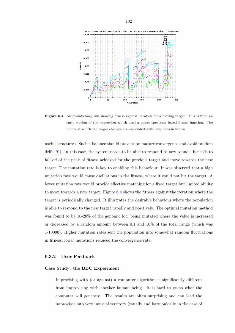
132

Figure 6.4: An evolutionary run showing fitness against iteration for a moving target. This is from an

early version of the improviser which used a power spectrum based fitness function. The

points at which the target changes are associated with large falls in fitness.

useful structures. Such a balance should prevent premature convergence and avoid random

drift [91]. In this case, the system needs to be able to respond to new sounds; it needs to

fall off of the peak of fitness achieved for the previous target and move towards the new

target. The mutation rate is key to enabling this behaviour. It was observed that a high

mutation rate would cause oscillations in the fitness, where it could not hit the target. A

lower mutation rate would provide effective matching for a fixed target but limited ability

to move towards a new target. Figure 6.4 shows the fitness against the iteration where the

target is periodically changed. It illustrates the desirable behaviour where the population

is able to respond to the new target rapidly and positively. The optimal mutation method

was found to be 10-20% of the genomic loci being mutated where the value is increased

or decreased by a random amount between 0.1 and 10% of the total range (which was

1-10000). Higher mutation rates sent the population into somewhat random fluctuations

in fitness, lower mutations reduced the convergence rate.

6.3.2 User Feedback

Case Study: the BBC Experiment

Improvising with (or against) a computer algorithm is significantly different

from improvising with another human being. It is hard to guess what the

computer will generate. The results are often surprising and can lead the

improviser into very unusual territory (tonally and harmonically in the case of

133

the BBC experiment.) Human logic and algorithmic/computer logic feel very

different. Finn Peters, 2010 [95].

The musician who has improvised with the system the most is saxophonist, flautist and

composer Finn Peters. Finn has a varied background, ranging from his work with contem-

porary classical group Nosferatu, through extensive jazz experience 2 and more mainstream

work with the likes of Sam Rivers [90, 27]. The above quote was provided by Finn in re-

sponse to the author’s request for feedback on a duet recorded for BBC Radio 3’s ‘jazz

on 3’ programme in 2009, featuring Finn on flute and unattended algorithm. The duet is

available on the CD included with this thesis (appendix A).

For this session, the timbral output of the improviser was deliberately constrained to

mild variations of a toned percussion-like sound, as Finn wanted to play a fairly melodic

piece. The algorithm operator (the author) started the program then left the machine

completely alone for the duration of the piece. Finn initially threaded a gentle mixture

of long notes, deliberately leading the algorithm to a similar output. This continued for

a while until the algorithm began to reprocess the notes in a sufficiently interesting way

such that it demanded that Finn responded to it. Then the line between Finn’s input and

the machine’s began to blur. The piece has an interesting and unpredictable ebb and flow

until it reaches a natural end point, when the author quickly stopped the algorithm. This

session was listed as one of the best live sessions recorded for that programme in 2009 [28].

This success is rather surprising - a completely automated program was able to compete

with jazz musicians from around the world and to produce output of sufficient quality to

be placed on this list. The author feels this can be considered a great success. Linking

back to Bown and Lexer’s work where they discuss the idea that a skilled improviser can

guide a much simpler algorithm through its state space, how much of this success should

be attributed to Finn and how much to the algorithm design [11]? Finn states in the

quote that [the algorithm] ‘can lead the improviser into very unusual territory (tonally

and harmonically...)’, which begs the question - who was leading whom? Whilst the human

player clearly carefully selected notes they knew would be likely to produce good results,

the re-arrangement of those notes is a joint effort. This is Young’s unimagined property

of live algorithms, where they might produce “a living computer music, an unimagined

music.” [145].

2His band, which now includes the author and associated algorithmic improvisers was rated as the BBC

best jazz band 2007

134

The Laptop Performer’s Perspective

From the perspective of the laptop operator, the use of live algorithms is an interesting de-

velopment from the more usual modes of laptop performance such as the manipulation of

effects, samples and synthesizers. In this recording session, the author deliberately pressed

the start button for the algorithm in an exaggerated fashion and stepped away from the

machine, to emphasise its autonomy. As an approach to live performance, this might seem

a bit limiting; so how might an operator interact more effectively with a live algorithm?

Live coding techniques allow the laptop musician to engage in a native way with a live al-

gorithm, by altering its processes at the logical, code level [22, 82, 89]. An example might

be the deliberate adjustment of the weighting used to vary the algorithm’s behaviour or

the on the fly adjustment of genetic algorithm parameters. Indeed, the algorithm itself

might be completely re-programmed on the fly. A typical group performance scenario for

the author would be to improvise by running several different algorithms simultaneously,

where each is fed from a different member of the group. The laptop performer can then

choose which algorithm(s) is heard based on which is currently displaying the most inter-

esting behaviour. Interesting behaviour might be for example, highly dynamic behaviour,

producing output which effectively adds to the current mood or highly contrasting out-

put which might lead the overall improvisation in a new direction. Indeed, the performer

might allow all algorithms to run simultaneously, feeding back into each other, after Lewis’

‘co-dominance’ method of improvisation [71].

Further Insights

Finn has provided more insights informally. He reports a ‘chicken and egg’ sensation where

over time, the line between what he has played and what the software has played becomes

blurred. He is responding to it responding to him responding to it ... Finn is clearly

able to distinguish between, to respond to and even to induce the different modes of the

improviser. For example, at the beginning of an improvisation he might play long, tonally

proximal notes to initialise the memory and induce slow, polyphonic playing, then later

on he might play rapid, varied notes to trigger the same on the part of the algorithm.

Indeed, Finn reports that part of the challenge and enjoyment when playing with such

systems is to try to figure out what the behaviour actually is. This connects directly to

Young’s opaque and intimacy attributes - algorithm design is a subtle blend of opacity and

intimacy, where the human improviser feels they are sharing a space with the algorithm

but it is not simply parroting their movements in that space; instead it has an element of

135

mystery or unpredictability.

In terms of the specifics of the sound synthesis and timbre matching, Finn found that a

completely free timbre search was quite challenging to play against, preferring using an FM

synthesis algorithm which had the frequency ratios quantised to increase the harmonicity

of the tones. Finn did not request this specific technical adjustment, that was the author’s

interpretation of how to fix this problem. It is possible that this situation would be less

problematic if the system were optimised for faster evolution. If tone matching could

be achieved in near real time, the musician would have more control when guiding the

tonality of the overall piece. The limitation of a requirement for harmonicity is not such a

problem as a large range of harmonic timbres are available. Perhaps the problem is that it

is more challenging to work expressively in series of timbres than series of notes and this

situation is exasperated if the timbre matching is too slow.

The system has inspired Finn to embark on compositional projects where algorithms

have been much more involved. The ‘Music of the Mind’ project looked at different ways

of mapping brain waves into the musical domain as well as ways of modelling musical

behaviours. The project included the improviser described here as well as subsequent

designs using Markov chains, where the note sequences were analysed in a Markovian

fashion to elicit their statistical interval and rhythmic relationships. On the ‘Music of the

Mind’ album, the improviser can be heard towards the end of the track ‘Sleep Music II’,

half way through the track ‘Oxygen’ and, possibly the best example, at the end of the

track ‘Brain Solo’, where it improvises a melody using an evolved saxophone-like sound

played using an FM synthesizer. A Markov chain driven rhythm synthesizer can be heard

during the track ‘Brain Solo’ [96].

6.4 Conclusion

A creative application of genetic algorithm driven tone matching has been presented.

The resulting system is an autonomous improviser which is designed to play alongside

human musicians. The four parts constituting the improviser have been described in detail,

namely, the synthesis engine, the tone matching algorithm, the listener and the improviser.

The demands placed on the GA design by the moving target problem have been discussed

and the mutation rate has been highlighted as the key algorithmic parameter here. The

system has been evaluated mainly on its artistic merit, since it includes components which

have been technically assessed in previous chapters. The properties of the system such

as its variable polyphony, octave ranges and note speed provide it with a wide melodic

136

and rhythmic scope which affords an intriguing behaviour for human musicians. It can

carry out intimate playing and less predictable playing, with its use of short and long term

memories. The ability to change the synthesis engine allows it to be easily adapted for

different scenarios. The system has proved to be a successful ‘musician’, being invited to

perform alongside leading musicians from the UK jazz scene 3.

3It is not clear if it is allowed to join the Musicians’ Union, however.

137

Chapter 7

Conclusion

In this final chapter, the thesis is drawn to a close. The solutions to problems and answers

to questions posed in the introduction are provided from the work in the thesis where

possible; unanswered questions are also highlighted. The contributions made by this

thesis are listed and references are made to the specific points in thesis at which they were

made. Directions for future work are outlined, dealing with the work from each chapter

in turn. Finally, there is a summary.

7.1 Research Questions

In this section, the problems and questions posed in the introduction are revisited; solu-

tions and answers are derived from the results reported in the thesis.

Problem 1: Numerical Representations of Timbre

An analysis of the ascending auditory pathway suggests distinct properties of an ideal

numerical representation of timbre. It should be multidimensional, aware of non-linear

features of human hearing and capable of differentiating typical variations such as bright-

ness and nasality. If this measure is to be used for efficient timbral comparisons, it should

also be orthogonal within itself, such that it is compact. Lastly, it should be able to

change gradually with variations in timbre. It has been shown that the MFCC fits with

these criteria: it is multidimensional, perceptually weighted (with its use of the Mel filter

bank and logarithmic power readings), capable of measuring typical timbral attributes (as

evidenced by the similarity of the MDS plots shown in figures 2.1 and 2.9, orthogonal (as

a result of the DCT stage) and finally its values vary gradually as the timbre changes

(as evidenced by the error surface plots from chapter 3 as well as the results reported by

138

Terasawa et al [121]). The successful application of the MFCC to speech recognition and

timbre classification problems supports its computational viability. Open source MFCC

extractors are available and their implementations, whilst they vary in certain details, gen-

erally produce similar output. A novel, reference implementation has been produced for

ease of programmatic integration and as a means to fully understand the computational

requirements.

Problem 2: Effective Sound Synthesizer Programming

A user trial was carried out which aimed to compare the synthesizer programming abilities

and behaviour of human and machine (chapter 4). In the first regard, the comparison of

abilities, the genetic algorithm tone matching technique used in the SynthBot software

proved to be a superior synthesizer programmer than the expert users involved in the

trial, at least as measured by the MFCC error metric. The human programmers were

able to program the subtractive synthesizer better than the FM synthesizer, achieving

scores which were within 50% of the machine in the former and an order of magnitude

worse than the machine in the latter case. Perhaps this supports the widely held opinion

that analog-style synthesizers are more intuitive to program than FM synthesizers. The

humans were able to program sounds which were reminiscent of the target sounds in most

cases, evidenced by the author listening to the sounds, but this perceptual similarity has

not been experimentally validated. An examination of the programming behaviour of the

humans showed that they tend to work with a single parameter at a time, exploring its

full range before moving to another. It seems that this strategy will become ineffective

once the number of parameters and the complexity of the synthesizer is too high. Also,

this will not work well for parameters which are highly interdependent as a parameter

thought fully explored might effectively change its function whilst another parameter is

being explored. It is worth noting that not all musicians who use synthesizers will have

anywhere near the skill of those involved in the trial and that even within this skilled

group, there was a wide variation in programming success. The best scores, especially

with the subtractive synthesizer, were impressive but the average scores were much less

so. In conclusion, human programmers seem to be able to program synthesizers with

greater precision than expected and are able to find near optimal settings in some cases,

given a synthesizer that is regarded as ‘intuitive’. It is not clear that this programming

success extends to cover more complex synthesizers however and not all synthesizer users

are likely to have such a skill level. There is clearly a need for more effective ways to

139

program synthesizers if the average user is to escape from the presets.

Problem 3: Mapping and Describing Sound Synthesis Space

A detailed description of the effect of parametric variations upon the output of various

sound synthesis algorithms has been provided in chapter 3. The concept of a timbral error

surface was introduced wherein the effect of parametric variation is presented as movement

in timbre space away from a reference point (subsection 3.2.1). These error surfaces are a

way of mapping sound synthesis space which can provide an insight into the best method

to use to search this space algorithmically. They also suggest appropriate resolutions for

sampling sound synthesis space and illustrate the timbral behaviour of different types of

parameter, e.g. quantised and continuous parameters.

The SoundExplorer tool is proffered as a system which provides its user with a dimen-

sionally reduced map showing the timbre space of a sound synthesis algorithm or a set

of audio files (section 2.5). Users can interactively explore the map, by playing back the

audio files or synthesizing the sounds in real time with parametric interpolation from one

position to the next. Whilst the tool has not been formally trialled, e.g. using a ‘find a

sound’ task, the initial reaction by users is that it is very exciting to be able to see all of

the sounds a synthesizer can make in a single window. It also provides a way of quickly

viewing the intersection between the sound space of different synthesizers or synthesizers

and real instruments and so on. With error surfaces and SoundExplorer, it is possible to

examine the details of the surface of sound synthesis space and to present an overview of

the complete space.

Problem 4: Searching Sound Synthesis Space or Automated Synthesizer

Programming

An extensive comparison of 4 methods through which sound synthesis space might be

automatically explored was presented in chapter 3. The 4 methods were feed forward

neural networks, genetic algorithms, hill climbing and a data driven approach. The aim

was to search for sounds which were known to reside in the space and for real instrument

sounds, where their residence in the space was an unknown. It was shown that the genetic

algorithm carried out the highest quality search but the hill climbing and data driven

approaches were also quite effective. The neural network showed very poor performance,

failing to learn a mapping between MFCC feature frames and synthesizer parameter set-

tings. This is unfortunate as the neural network is the only one of these methods that could

140

operate in real time, compared to the 60 seconds or more required by the other methods

to match a timbre. A hybrid data driven/ genetic algorithm approach is presented and

shown to have superior performance than either of its individual parts. It is felt that with

optimisation of the data driven approach, this could provide much faster tone matching.

Fixed architecture FM synthesis, modelled after the Yamaha DX7, offered the best tone

matching performance over the real instrument data set. The poor ability of the genetic

algorithm and other approaches to program the variable architecture FM synthesis algo-

rithm was quite disappointing as it was felt that this synthesis algorithm should offer the

best range of sounds and is also perhaps the hardest for a human to program. Further, in

previous work by the author which partly inspired this thesis, a variable architecture syn-

thesis algorithm proved itself capable of generating a huge variety of sounds when placed

in an interactive GA context [136]. The topic in general warrants much further study,

both in terms of optimisation performance and synthesis architectures. The ultimate goal

is to produce a real time tone matcher that can work with any sound synthesis algorithm.

This possibility is discussed further in section 7.3.

Problem 5: Creative Applications of the Above

Four creative applications of sound synthesis space search have been described. Sound-

Explorer is a synthesizer programming interface that does away with the usual ideas of

categories and presets and instead presents the user with an intriguing image showing a

large range of timbres that the synthesizer can make (section 2.5). The user can zoom into

the image to explore heavily populated parts of the space and they can combine different

sound sets, e.g. two synthesizers or a synthesizer and a set of samples from a sample

library. The system provides a form of parametric interpolation which allows the user to

hear the sound of the space between sounds. Formal user trials would inform the future

development of this project, but as it stands it is an interesting tool to interact with, which

provides a means to aggressively explore sound synthesis space. SynthBot aims to allow its

users to escape from the presets and to specify the sound they want directly, by example,

in the form of an audio file (chapter 4). User trials pitting SynthBot against human pro-

grammers showed that SynthBot is a very effective automated synthesizer programmer;

as a studio tool, it is the equivalent or better of having an expert human synthesizer pro-

grammer at your disposal. The process of creating a commercial implementation of this

system is ongoing. The Evolving Drum Machine attempts to re-invigorate the venerable

drum machine by providing a means of generating timbral transitions for the percussion

141

sounds (chapter 5). This is an attempt to take the idea of complete timbral control from

electroacoustic music and bring it to the drum machine, a fixed timbred stalwart of ‘pop-

ular’ electronic music. The system was trialled with two experienced drum machine users

and the response was very positive. They engaged conceptually with the idea of evolving

timbres but did state the importance of retaining some sort of editorial control. The final

application was the timbre matching improviser, presented in chapter 6. This system has

been used extensively for live recordings and has appeared on national radio, where it

achieved some plaudits. The musician who has played the most with this system states

that is enables him to explore tonal and harmonic spaces he would not otherwise have

entered and that the output is often surprising. This system succeeds by relying on the

skilled musician to provide harmonic and timbral direction yet not mimicking them too

directly. This balance of the feeling of interactivity with the ability to surprise and lead

is a key challenge in live algorithm work.

7.2 Contributions

In the introduction section 1.3 a list of contributions made by this thesis was provided.

The list is repeated here with some comments and references to the relevant points in the

thesis.

1. An assertion of the validity of the Mel Frequency Ceptstrum Coefficient as a timbral

descriptor.

This contribution is comprised of the description of an ideal numerical measure of

timbre found in section 2.3 and the review of previous work using the MFCC for

timbre classification found in subsection 2.4.2.

2. A comparison of open source MFCC extractors.

This contribution is provided as the reported results of a code and performance level

comparison of 4 open source extractors in subsection 2.4.3.

3. New methods for describing, visualising and exploring timbre spaces.

The SoundExplorer tool described in section 2.5 allows its user to explore the com-

plete timbre space of a synthesizer, or any set of audio files. The concept of a timbral

error surface introduced in section 3.2 offers a new means of visualising movement

through timbre space from a reference point. Detailed descriptions of timbre space

are provided in subsection 3.2.1.

142

4. A comparison of methods for automatically searching sound synthesis space.

Chapter 3 provides this comparison, wherein a genetic algorithm, a neural network,

a hill climber and a data driven approach are compared in their ability to search

sound synthesis space.

5. A synthesis algorithm-agnostic framework for automated sound synthesizer program-

ming compatible with standard studio tools.

The SynthBot system described in chapter 4 is just such a framework. It can interact

with any synthesizer which is compatible with the VSTi standard, as long as it

exposes its full parameter set in the standard way.

6. A comparison of human and machine synthesizer programming.

SynthBot was evaluated by comparing its synthesizer programming performance

to that of 10 expert humans. Human synthesizer programming behaviour was also

compared to the machine’s in terms of the parametric trajectories taken. The results

of these comparisons can be found in subsection 4.4.2.

7. A re-invigorated drum machine.

A fresh take on the idea of a drum machine is provided in the form of the evolving

drum machine in chapter 5. Trials with two experienced drum machine users indi-

cated that the system was interesting and did provide a new mode of interaction,

where the relinquishing of a certain amount of control to the machine yielded useful

creative results.

8. A timbre matching, automated improviser.

The timbre matching techniques reported throughout the thesis are deployed as part

of an autonomous, improvising agent in chapter 6. The agent has been successfully

used in recording and radio sessions as well as many live performances.

7.3 Future Work

Much future work is suggested by this thesis. In this section, this will be discussed chapter

by chapter.

143

7.3.1 Chapter 2

Chapter 2 covers quite a range of material and as such suggests several interesting direc-

tions. New methods of sound synthesis based around sparse coding schemes are discussed

but the new vistas of synthesized sound opened up by these schemes have yet to be fully

explored. The compact representations of sounds made possible by these schemes also

seem to lend themselves to the goal stated earlier, of a real time tone matcher with a

sophisticated and flexible sound synthesis engine.

It would be interesting to repeat some of the listener based experiments discussed

in chapter 2, or to obtain the data, and compare the similarity judgements to those of

numerical measures such as the MFCC. One outcome of this would be a ground truth for

timbre similarity against which numerical measures could be compared.

The SoundExplorer tool, which aims to present maps of sound synthesis space to the

user for exploration, could be extended through the use of cluster analysis. Whilst the mul-

tidimensional scaling approach appears to work, in that similar sounds are close together,

a cluster based approach would allow the sounds to be grouped in high dimensional space

and subsequently presented as clusters in a lower dimensional space. It might be possible

to extract the ‘canonical presets’ for a synthesizer in this way, as they would be the cluster

centres. Whilst the SoundExplorer tool is interesting to users, it has not been objectively

established if it actually enables them to search synthesis space more effectively than a

standard ‘knobs and sliders’ interface. This could be tested by providing users with three

interfaces: standard SoundExplorer, SoundExplorer with the sounds placed at random

positions and something like the SynthBot interface. They would then be set the task of

programming several sounds in a limited time. Their success could be measured using the

MFCC distance metric.

7.3.2 Chapter 3

Much future work is suggested by this study. Further analysis of error surfaces, including

different synthesis algorithms; better modelling of commercially available synthesizers.

or direct use of them via the SynthBot software; the analysis of synthesizer parametric

redundancy; establishing why some parameter settings are harder to find than others;

further optimisation of the data driven search and genetic algorithm; further investigation

of the application of variable architecture synthesis algorithms; investigation of more real

time sound matching techniques, to fill in where the neural network failed. The author is

in the process of preparing the software used to conduct the study for public release as an

144

extension for the SuperCollider language, known as a Quark.

7.3.3 Chapter 4

The SynthBot system has a lot of potential and this initial trialling and analysis suggests

several next steps for its technical development. A more extensive test of SynthBot’s

performance across a range of different VSTi plug-ins could be carried out, including its

use with chains of plug-ins (returning to the idea of variable architecture sound synthesis).

The results of the human vs machine synthesizer programming trial could be re-analysed

using a human derived similarity metric. This could be done by means of an on-line survey

where the subjects are played pairs of sounds from the experiment and asked to judge the

similarity using, for example, a Likert scale. A further extension to the programming part

of the trial would be to set a similar sound matching task but to include more methods for

programming the synthesizers, including SoundExplorer, interactive GAs and a category

based interface like those described in subsection 4.1.1. The author has recently been in

communication with the authors of another VSTi programmer with an aim to developing

a collaborative project [44].

7.3.4 Chapter 5

Chapter 5 mentions linear separability, where the use of an island population model enables

separate parts of the sound to be matched in parallel. An analysis of the linear separability

of sound synthesis parameters, including epistatic effects would be interesting. Do different

‘genes’ appear to encode different parts of the sound, for example? This information

could then be used to improve the tone matching performance with variable architecture

synthesizers, where modules which match different parts of the desired sound would be

evolved in isolation then recombined.

7.3.5 Chapter 6

The improvising system presented in chapter 6 could be extended in many ways. Real time

timbre matching would be a highly desirable next step. This could potentially be achieved

using a pre-evolved database of parameter settings. In this case, the database would be

evolved offline to match a variety of common musical timbres (e.g. timbres derived from

acoustic instruments). Clustering could be used to limit the size of the database or it

might be filtered to only include a certain instrument. For live performance, the closest

available match to the current timbre from the live musician could be quickly found from

145

the limited database. Or indeed, the worst match for an interesting effect! If the timbral

output of the live musician can thus be characterised as a stream of a limited number of

states, it could be represented using a statistical technique such as a Markov chain. New

streams of timbres could be generated which are statistically similar to the live performer’s

output. This might be called statistical, parametric, concatenative resynthesis.

7.4 Summary

... a ‘living’ computer music might be even more apposite, permanently explor-

ing all elements of its emergent language, and in real-time, not just in concept.

Young 2007 [145].

In this thesis, the concept of automatic sound synthesizer programming has been explored

in depth. Automatic sound synthesizer programming is the removal of the requirement for

the user of a synthesizer to explicitly specify its parameter settings. Solutions include the

provision of a bank of presets, the presentation of the space of possible sounds a synthesizer

can make and the search of this space for specific target sounds. The sound made by a

synthesizer can be described numerically using Mel Frequency Cepstral Coefficients, which

provide a combination of a track record of successful applications to timbre related tasks,

efficient computation and wide applicability. The SoundExplorer tool presents the user

with a dimensionally reduced view of the sounds that a synthesizer can make, mapped out

in MFCC timbre space such that similar sounds are close together. The user can explore

the space, synthesizing and interpolating between the sounds in real time. Techniques for

automatically searching sound synthesis space include genetic algorithms, hill climbers,

data driven approaches and neural networks. It has been shown that the first three all

provide reasonable tone matching performance but that the genetic algorithm offers the

most effective search. With the use of an automated programmer, FM synthesis modelled

after the venerable Yamaha DX7 is an effective means of synthesizing a variety of real

instrument tones. SynthBot is a studio tool which is capable of automatically matching

target sounds using VSTi compatible virtual synthesizers. It performs better at this task

than expert human users, though their performance was in itself impressive. The inclusion

of automated timbral exploration capabilities into a drum machine makes for an interesting

and creative experience for musicians, beyond that provided by a standard drum machine

and warrants further developments. The genetic algorithm’s parameters and their effect

upon search behaviour can be viewed in a different light if the priority is not the best

146

search, but an artistic exploration of the search trajectory. In this case, mutation rates

and types have a significant impact. A timbre matching improviser has been created which

has inspired a musician who has played with it to embark on new projects which explicitly

engage with and fund the ideas of autonomous musical agents. The automated improviser

continues to appear in live performances and radio broadcasts, most recently in January

2011.

147

Bibliography

[1] N. Y. Abrams. Method for automatic sound synthesis, US patent number 5900568,

May 1999. http://www.freepatentsonline.com/5900568.html. 5

[2] L. J. S. M. Alberts. Sound reproduction using evolutionary methods: A comparison

of FM models. Website, 2005. www.math.unimaas.nl/personal/ronaldw/PhDMaBa-

teaching/GraduationStudents/Ba/LaurensAlbertsBaFINAL2005.pdf. 84

[3] Jens M. Andreasen. Phase modulation, 2010.

http://en.wikipedia.org/wiki/Phase modulation. 49

[4] Arturia. Arturia analog factory, 2010. http://www.arturia.com/. 5, 83

[5] A. Lynne Beal. The skill of recognizing musical structures. Memory & Cognition,

13(5):405–412, 1985. 20, 21

[6] James Beauchamp, editor. Analysis, Synthesis, and Perception of Musical Sounds:

The Sound of Music (Modern Acoustics and Signal Processing). Springer, 1 edition,

December 2006. http://www.worldcat.org/isbn/0387324968. 4, 22

[7] Ross Bencina. The metasurface - applying natural

neighbour interpolation to Two-to-Many mapping, 2005.

http://citeseerx.ist.psu.edu/viewdoc/summary?doi=10.1.1.59.2845. 5, 39, 40,

85

[8] J. A. Biles. GenJam in perspective: a tentative taxonomy for GA music and art

systems. Leonardo, 36(1):43–45, 2003. 123

[9] T. Blackwell and M. Young. Live algorithms. Artificial Intelligence and Simulation

of Behaviour Quarterly, 122:7–9, 2005. 123

[10] B. Bogert, M. Healy, and J. Tukey. The quefrency alanysis of time series for echoes:

Cepstrum, pseudo-autocovariance, cross-cepstrum and saphe cracking. In Proc.

Symp. on Time Series Analysis, pages 209–243, 1963. 27

148

[11] Oliver Bown and Sebastian Lexer. Continuous-time recurrent neural networks for

generative and interactive musical performance. In EvoWorkshops, pages 652–663,

2006. 124, 133

[12] Ollie Bown, Ben Porter, and Benito. The beads project, 2008.

http://www.beadsproject.net/. 4, 31

[13] Kevin J. Brewer. IEEE-754 references. Website, January 2009.

http://babbage.cs.qc.edu/courses/cs341/IEEE-754references.html. 57

[14] J. C. Brown, O. Houix, and S. McAdams. Feature dependence in

the automatic identification of musical woodwind instruments. The Jour-

nal of the Acoustical Society of America, 109(3):1064–1072, March 2001.

http://view.ncbi.nlm.nih.gov/pubmed/11303920. 30

[15] Jamie Bullock. LibXtract: A lightweight library for audio feature extraction. In Pro-

ceedings of the International Computer Music Conference, Copenhagen, Denmark,

2007. ICMA. 4, 31

[16] M. A. Casey, R. Veltkamp, M. Goto, M. Leman, C. Rhodes, and

M. Slaney. Content-based music information retrieval: Current directions

and future challenges. Proceedings of the IEEE, 96(4):668–696, March 2008.

http://dx.doi.org/10.1109/JPROC.2008.916370. 4, 30

[17] Gal Chechik, Michael J. Anderson, Omer Bar-Yosef, Eric D. Young, Naf-

tali Tishby, and Israel Nelken. Reduction of information redundancy in

the ascending auditory pathway. Neuron, 51(3):359–368, August 2006.

http://dx.doi.org/10.1016/j.neuron.2006.06.030. 18

[18] Michael Chinen and Naotoshi Osaka. Genesynth: Noise band-based genetic algo-

rithm analysis/synthesis framework. In Proceedings of the ICMC 2007 International

Computer Music Conference, 2007. 6, 84

[19] John Chowning and David Bristow. FM Theory and Applications: By Musicians for

Musicians. Hal Leonard Corp, 1986. http://www.worldcat.org/isbn/4636174828. 49

[20] E. Ciurana. Developing with Google App Engine. Springer, 2009. 102

[21] N. Collins. Reinforcement learning for live musical agents. In Proceedings of

ICMC2008, International Computer Music Conference, Belfast. Citeseer, 2008. 8

149

[22] N. Collins, A. McLean, J. Rohrhuber, and A. Ward. Live coding in laptop perfor-

mance. Organised Sound, 8(03):321–330, 2003. 134

[23] Nick Collins. Experiments with a new customisable interac-

tive evolution framework. Org. Sound, 7(3):267–273, 2002.

http://dx.doi.org/http://dx.doi.org/10.1017/S1355771802003060. 5, 124

[24] Nick Collins. Towards Autonomous Agents for Live Computer Music: Realtime

Machine Listening and Interactive Music Systems. PhD thesis, Centre for Science

and Music, Faculty of Music, University of Cambridge, 2006. 2, 7, 8, 123

[25] Nick Collins. MFCC UGen for SuperCollider, 2010.

http://supercollider.svn.sourceforge.net/supercollider/. 4, 31

[26] Nick Collins and Chris Kiefer. NeuralNet: a language side neural network class for

SuperCollider. http://www.informatics.sussex.ac.uk/users/ck84/index.php, 2009.

66

[27] The British Broadcasting Corporation. BBC jazz awards, July 11th 2007, 2008.

http://www.bbc.co.uk/music/jazzawards2007/winners.shtml. 133

[28] The British Broadcasting Corporation. Best sessions of 2009, 2009.

http://www.bbc.co.uk/programmes/b00pdwgn. vi, 133

[29] Robert G. Crowder. Imagery for musical timbre. Journal of Ex-

perimental Psychology: Human Perception and Performance, 15(3),

1989. http://www.sciencedirect.com/science/article/B6X08-46X8WS6-

5/2/160555580345be7f7ed9e10bd66c779e. 4, 20, 21, 22

[30] Palle Dahlstedt and Clavia. Nord Modular G2 patch mutator. website, 2006.

http://www.clavia.se/products/nordmodular/MutatorManual.pdf. 5, 84

[31] S. Davis and P. Mermelstein. Comparison of parametric representa-

tions for monosyllabic word recognition in continuously spoken sen-

tences. Acoustics, Speech, and Signal Processing [see also IEEE Trans-

actions on Signal Processing], IEEE Transactions on, 28(4):357–366, 1980.

http://ieeexplore.ieee.org/xpls/abs all.jsp?arnumber=1163420. 4, 26

[32] Diana Deutsch, editor. The Psychology of Music, Second Edition (Academic Press

Series in Cognition and Perception). Academic Press, 2 edition, October 1998.

http://www.worldcat.org/isbn/0122135652. 4, 17, 19, 20

150

[33] Antti Eronen. Comparison of features for musical instrument recognition. In In

Proc. IEEE Workshop on Applications of Signal Processing to Audio and Acoustics,

2001. http://citeseerx.ist.psu.edu/viewdoc/summary?doi=10.1.1.74.2098. 4, 30

[34] Slim Essid and GaAl Richard. Musical instrument recognition based on class pairwise

feature selection. In in 5th International Conference on Music Information Retrieval

(ISMIR, 2004. 65

[35] Imola Fodor. A survey of dimension reduction techniques, 2002.

http://citeseerx.ist.psu.edu/viewdoc/summary?doi=10.1.1.8.5098. 5

[36] M. Frigo and S. G. Johnson. The design and implementation of FFTW3. Proceedings

of the IEEE, 93(2):216–231, February 2005. http://www.fftw.org/. 32

[37] Lawrence Fritts. The University of Iowa Electronic Music Studios musical instrument

samples, April 2005. http://theremin.music.uiowa.edu/MIS.html. 55, 65

[38] Todor Ganchev, Nikos Fakotakis, and George Kokkinakis. Comparative

evaluation of various MFCC implementations on the speaker verification

task. In in Proc. of the SPECOM-2005, volume 1, pages 191–194, 2005.

http://citeseerx.ist.psu.edu/viewdoc/summary?doi=10.1.1.75.8303. 28, 30

[39] R. Garcia. Growing sound synthesizers using evolutionary methods. In Proceedings

of ALMMA 2002 Workshop on Artificial Models for Musical Applications, pages

99–107. Citeseer, 2001. 6

[40] A. Gounaropoulos and C. Johnson. Timbre interfaces using adjectives and adverbs.

In Proceedings of the 2006 International Conference on New Interfaces for Musical

Expression, pages 101–102, 2006. 6

[41] J. C. Gower. Some distance properties of latent root and vector methods

used in multivariate analysis. Biometrika, 53(3-4):325–338, December 1966.

http://dx.doi.org/10.1093/biomet/53.3-4.325. 39

[42] John M. Grey. Multidimensional perceptual scaling of musical timbres.

The Journal of the Acoustical Society of America, 61(5):1270–1277, 1977.

http://dx.doi.org/10.1121/1.381428. xiv, 5, 23, 24

[43] Andrea R. Halpern, Robert J. Zatorre, Marc Bouffard, and Jen-

nifer A. Johnson. Behavioral and neural correlates of perceived and

151

imagined musical timbre. Neuropsychologia, 42(9):1281–1292, 2004.

http://dx.doi.org/10.1016/j.neuropsychologia.2003.12.017. xiv, 4, 5, 22, 24,

25, 65, 102

[44] Sebastian Heise, Michael Hlatky, and Jorn Loviscach. Automatic cloning of recorded

sounds by software synthesizers. In Audio Engineering Society Convention 127, 2009.

http://www.aes.org/e-lib/browse.cfm?elib=15053. 84, 85, 92, 144

[45] Matthew Herbert. Personal contract for the composition of music [incorporating the

manifesto of mistakes]., 2005. http://www.matthewherbert.com/pccom.php. 8

[46] J. H. Holland. Adaptation in natural and artificial systems. MIT Press Cambridge,

MA, USA, 1992. 124

[47] Karen Holtzblatt and Hugh Beyer. Making customer-centered

design work for teams. Commun. ACM, 36(10):92–103, 1993.

http://dx.doi.org/http://doi.acm.org/10.1145/163430.164050. 14, 119

[48] A. Horner, J. Beauchamp, and L. Haken. Genetic Algorithms and Their Application

to FM, Matching Synthesis. Computer Music Journal, 17(4):17–29, 1993. 6, 84, 114

[49] Tomas Hromadka, Michael R. DeWeese, and Anthony M. Zador. Sparse representa-

tion of sounds in the unanesthetized auditory cortex. PLoS Biol, 6(1):e16+, January

2008. http://dx.doi.org/10.1371/journal.pbio.0060016. 19

[50] W. Hsu. Using timbre in a computer-based improvisation system. In Proceedings of

the ICMC, pages 5–9, 2005. 7

[51] William Hsu. Two approaches for interaction management in timbre-aware impro-

visation systems. In International Computer Music Conference, Belfast 2008, 2008.

7

[52] R. Ihaka and R. Gentleman. R: a language for data analysis and graphics. Journal

of computational and graphical statistics, 5(3):299–314, 1996. 13

[53] Muse Research Inc. KVR: Audio plug-in database, 2010.

http://www.kvraudio.com/. 38, 86

[54] Native Instruments. FM8 the power of digital. Website, 2008. http://www.native-

instruments.com/index.php?id=fm7 us. 83

[55] Native Instruments. Absynth 5 Manual, 2010. 84

152

[56] Native Instruments. Native Instruents’ Kore 2, 2010. http://www.native-

instruments.com/#/en/products/producer/kore-2/. 5, 83

[57] P. Iverson and C. L. Krumhansl. Isolating the dynamic attributes of musical timbre.

The Journal of the Acoustical Society of America, 94:2595, 1993. xiv, 4, 5, 23, 24

[58] J. H. Jensen, M. G. Christensen, and S. H. Jensen. A framework for analysis of

music similarity measures. In Proc. European Signal Processing Conf, pages 926–

930. Citeseer, 2007. 31

[59] C. G. Johnson. Exploring sound-space with interactive genetic algorithms. Leonardo,

36(1):51–54, 2003. 5, 124

[60] Colin G. Johnson and Alex Gounaropoulos. Timbre interfaces using adjectives and

adverbs. In NIME ’06: Proceedings of the 2006 conference on New interfaces for

musical expression, pages 101–102, Paris, France, France, 2006. IRCAM — Centre

Pompidou. http://portal.acm.org/citation.cfm?id=1142215.1142239. 85

[61] S. A. Kauffman. The origins of order: Self-organization and selection in evolution.

Oxford University Press, USA, 1993. 54

[62] Paul Kellet. mda-vst.com. website, 2008. http://mda.smartelectronix.com/. xii, 86,

88

[63] R. A. Kendall, E. C. Carterette, and J. M. Hajda. Natural vs. synthetic instrument

tones. Music Perception, 16:327–364, 1999. 4, 25

[64] Stefan Kersten. skUG SuperCollider UGen library., 2008. http://space.k-

hornz.de/software/skug/. 48

[65] Syed A. Khayam. Seminar 1 the discrete cosine transform: Theory and application,

2003. 29

[66] Tomi Kinnunen and Paavo Alku. On separating glottal source and vo-

cal tract information in telephony speaker verification. Acoustics, Speech,

and Signal Processing, IEEE International Conference on, 0:4545–4548, 2009.

http://dx.doi.org/10.1109/ICASSP.2009.4960641. 29

[67] Yuyo Lai, Shyh-kang Jeng, Der-tzung Liu, and Yo-chung Liu. Automated

optimization of parameters for FM sound synthesis with genetic algorithms.

http://citeseerx.ist.psu.edu/viewdoc/summary?doi=10.1.1.127.2761. 6, 84, 85

153

[68] L. Lamport and D. Bibby. LATEX: A document preparation system, volume 260.

Citeseer, 1986. 13

[69] P. Langley, J. H. Gennari, W. Iba, California U. Information, and Science. Technical

hill-climbing theories of learning interim report, 1987. 65

[70] Charles C. Lee and S. Murray Sherman. Drivers and modulators in

the central auditory pathways. Frontiers in neuroscience, 4, 2010.

http://dx.doi.org/10.3389/neuro.01.014.2010. 17

[71] G. E. Lewis. Too many notes: Computers, complexity and culture in Voyager.

Leonardo Music Journal, pages 33–39, 2000. 123, 134

[72] S. Liang. Java Native Interface: Programmer’s Guide and Reference. Addison-

Wesley Longman Publishing Co., Inc. Boston, MA, USA, 1999. 13, 86

[73] L. Lin, E. Ambikairajah, and W. H. Holmes. Auditory filter bank design using

masking curves. In Eurospeech 2001, 2001. 18

[74] Beth Logan. Mel frequency cepstral coefficients for music modeling.

In In International Symposium on Music Information Retrieval, 2000.

http://citeseerx.ist.psu.edu/viewdoc/summary?doi=10.1.1.11.9216. 30

[75] Cristyn Magnus. Evolving electroacoustic music: the application of genetic algo-

rithms to time-domain waveforms. In Proceedings of the 2004 International Com-

puter Music Conference, pages 173–176, 2004. 118

[76] M. V. Mathews, J. E. Miller, F. R. Moore, J. R. Pierce, and J. C. Risset. The

technology of computer music. The MIT Press, 1969. 1

[77] J. McCartney. SuperCollider, a new real time synthesis language. In Proceedings of

the International Computer Music Conference, pages 257–258. INTERNATIONAL

COMPUTER MUSIC ACCOCIATION, 1996. 108

[78] James McCartney. Rethinking the computer music language:

SuperCollider. Computer Music Journal, 26(4):61–68, 2002.

http://dx.doi.org/10.1162/014892602320991383. 2, 3, 13

[79] J. McDermott, N. Griffith, and M. O’Neill. Evolutionary GUIs for sound synthesis.

Applications of Evolutionary Computing, pages 547–556, 2007. 124

154

[80] James M. McDermott. Evolutionary Computation Applied to Sound Synthesis. PhD

thesis, The University of Limerick, February 2008. 6

[81] D. McEnnis, C. McKay, and I. Fujinaga. jAudio: A feature extraction library. In

International Conference on Music Information Retrieval. Citeseer, 2005. 31

[82] A. McLean. Hacking Perl in nightclubs. at http://www. perl.

com/pub/a/2004/08/31/livecode. html, 2004. 134

[83] P. McLeod and G. Wyvill. A smarter way to find pitch. In Proceedings of Interna-

tional Computer Music Conference, ICMC, 2005. 129

[84] Paul Mermelstein. Distance measures for speech Recognition–Psychological and

instrumental. In Joint Workshop on Pattern Recognition and Artificial Intelligence,

1976. 26

[85] E. R. Miranda. At the crossroads of evolutionary computation and music: Self-

programming synthesizers, swarm orchestras and the origins of melody. Evolutionary

Computation, 12(2):137–158, 2004. 6

[86] E. R. Miranda. Evolutionary computer music. Springer Verlag, 2007. 6

[87] T. Mitchell, J. Charles, and W. Sullivan. Frequency Modulation Tone Matching

Using a Fuzzy Clustering Evolution Strategy. In AES 118th Convention, Barcelona,

Spain, 2005. 6

[88] Brian C. J. Moore. An Introduction to the Psychology of Hearing. Academic Press,

fifth edition, April 2003. http://www.worldcat.org/isbn/0125056281. 4, 16, 17

[89] C. Nilson. Live coding practice. In Proceedings of the 7th international conference

on New interfaces for musical expression, pages 112–117. ACM, 2007. 134

[90] Noszferatu. Noszferatu contemporary music collective. Website, 2010.

http://noszferatu.com/. 133

[91] G. Ochoa, I. Harvey, and H. Buxton. Error thresholds and their relation to optimal

mutation rates. Advances in Artificial Life, pages 54–63, 1999. 132

[92] B. A. Olshausen and D. J. Field. Emergence of simple-cell receptive field properties

by learning a sparse code for natural images. Nature, 381(6583):607–609, 1996. 19

155

[93] C. Pantev, M. Hoke, B. Lutkenhoner, and K. Lehnertz. Tonotopic organization of the

auditory cortex: pitch versus frequency representation. Science, 246(4929):486–488,

October 1989. http://dx.doi.org/10.1126/science.2814476. 18

[94] Finn Peters. Butterflies album released by accidental records, 2008. vi

[95] Finn Peters. Improvising with (or against) a computer algorithm is significantly

different from improvising with another human being. Personal communication,

December 2010. 133

[96] Finn Peters. Music of the mind album released by mantella records, 2010. vi, 135

[97] Mark A. Pitt and Robert G. Crowder. The role of spectral and

dynamic cues in imagery for musical timbre. Journal of Exper-

imental Psychology: Human Perception and Performance, 18(3),

1992. http://www.sciencedirect.com/science/article/B6X08-46V0CBH-

8/2/9b9f02c2984d9b7f591201700c0bd2fb. 4, 20, 21, 22

[98] M. Puckette. Max at seventeen. Computer Music Journal, 26(4):31–43, 2002. 2

[99] Lawrence Rabiner and Biing-Hwang Juang. Fundamentals of Speech

Recognition. Prentice Hall, united states ed edition, April 1993.

http://www.worldcat.org/isbn/0130151572. 27, 30

[100] Lawrence R. Rabiner and Ronald W. Schafer. Digital Processing

of Speech Signals. Prentice Hall, us ed edition, September 1978.

http://www.worldcat.org/isbn/0132136031. 27

[101] Gordon Reid. Synth secrets. Sound on Sound Magazine, 1999.

http://www.soundonsound.com/sos/allsynthsecrets.htm. 108

[102] Curtis Roads. The Computer Music Tutorial. The MIT Press, February 1996.

http://www.worldcat.org/isbn/0262680823. 8

[103] Martin Roth and Matthew Yee-King. A Java-based VST host, 2008.

http://github.com/mhroth/jvsthost. 86, 102

[104] R. Rowe. Interactive music systems: machine listening and composing. MIT Press

Cambridge, MA, USA, 1992. 6, 8, 122

[105] C. Scaletti. Computer music languages, Kyma, and the future. Computer Music

Journal, 26(4):69–82, 2002. 2, 3

156

[106] Markus Schedl. The CoMIRVA toolkit for visualizing music-related data. Technical

report, Department of Computational Perception, Johannes Kepler University Linz,

June 2006. 4, 31

[107] Simon Scholler and Hendrik Purwins. Sparse coding for drum sound classification

and its use as a similarity measure. In 3rd International Workshop on Machine

Learning and Music, 2010. 19

[108] Diemo Schwarz, Gregory Beller, Bruno Verbrugghe, Sam Britton, and Ircam Centre

Pompidou. Real-Time Corpus-Based concatenative synthesis with CataRT. In in

Proc. of the Int. Conf. on Digital Audio Effects (DAFx-06, pages 279–282, 2006. 6,

39

[109] X. Serra and J. Smith. Spectral modeling synthesis: A sound analysis/synthesis

system based on a deterministic plus stochastic decomposition. Computer Music

Journal, 14(4):12–24, 1990. 6

[110] Evan C. Smith and Michael S. Lewicki. Efficient auditory coding. Nature,

439(7079):978–982, February 2006. http://dx.doi.org/10.1038/nature04485. 19

[111] J. O. Smith. Viewpoints on the history of digital synthesis. In Proceedings of the

International Computer Music Conference, page 1, 1991. 1

[112] Steven W. Smith. The Scientist & Engineer’s Guide to Digital Signal Processing.

California Technical Pub., 1999. http://www.worldcat.org/isbn/0966017633. 29

[113] R. Stallman. Linux and the GNU project. Accessed at http://www. gnu.

org/gnu/linux-and-gnu. html March, 26, 2006. 13

[114] R. M. Stallman. EMACS the extensible, customizable self-documenting display edi-

tor. In Proceedings of the ACM SIGPLAN SIGOA symposium on Text manipulation,

pages 147–156. ACM, 1981. 13

[115] Steinberg. VST audio Plug-Ins SDK 2.4 revision 1. website, 2008.

http://www.steinberg.de/331+M52087573ab0.html. 13, 86

[116] S. S. Stevens, Je, and E. B. Newman. A scale for the measurement of the psycho-

logical magnitude of pitch. J. Acoust Soc Amer, 8:185–190, 1937. 26, 27

[117] D. Stowell. Making music through real-time voice timbre analysis: machine learning

and timbral control. PhD thesis, School of Electronic Engineering and Computer

157

Science, Queen Mary University of London, 2010. http://www.mcld.co.uk/thesis/.

5, 39

[118] Bob L. Sturm, Curtis Roads, Aaron Mcleran†, and John J. Shynk. Analysis, visu-

alization, and transformation of audio signals using dictionary-based methods. In

International Computer Music Conference, Belfast 2008, 2008. 6, 19

[119] SynthTopia. Synthtopia Roland TR-909, 2006.

http://www.synthtopia.com/synth review/RolandTR-909.html. 110

[120] T. Takala, J. Hahn, L. Gritz, J. Geigel, J. W. Lee, George W. Engineering, and

Science. Using physically-based models and genetic algorithms for functional com-

position of sound signals, synchronized to animated motion. In Proceedings of the

International Computer Music Conference, page 180. Citeseer, 1993. 124

[121] H. Terasawa, M. Slaney, and J. Berger. The thirteen colors of timbre. In Applica-

tions of Signal Processing to Audio and Acoustics, 2005. IEEE Workshop on, 2005.

http://ieeexplore.ieee.org/xpl/freeabs all.jsp?arnumber=1540234. 4, 25, 138

[122] B. Thom. BoB: an interactive improvisational music companion. In Proceedings of

the fourth international conference on Autonomous agents, pages 309–316. ACM,

2000. 123

[123] William F. Thompson. Music, Thought, and Feeling: Understanding

the Psychology of Music. Oxford University Press, USA, October 2008.

http://www.worldcat.org/isbn/0195377079. 4, 20

[124] Unknown. Vintage synth explorer, 2010. http://www.vintagesynth.com/. 83

[125] Various. UGen plugins for SuperCollider. http://sc3-plugins.sourceforge.net/, 2010.

http://sc3-plugins.sourceforge.net/. 129

[126] B. L. Vercoe and Others. Csound. Massachusetts Institute of Technology, 1993. 2

[127] G. Von Bekesy. Experiments in Hearing (Psychology). McGraw-Hill

Education, 1st, date same on title & copyright page edition, 1960.

http://www.worldcat.org/isbn/0070043248. 17

[128] Waldorf. Waldorf Attack Percussion Synthesizer.

http://www.waldorfmusic.de/en/products/attack, 2007. 108

158

[129] W. Walker, P. Lamere, P. Kwok, B. Raj, R. Singh, E. Gouvea, P. Wolf, and

J. Woelfel. Sphinx-4: A flexible open source framework for speech recognition.

Sun Microsystems, Inc. Mountain View, CA, USA, page 18, 2004. 31

[130] Paul White. Waldorf Attack review. Sound on Sound, 0, February 2002.

http://www.soundonsound.com. xvii, 109

[131] Darrell Whitley. The GENITOR algorithm and selection pressure: Why

Rank-Based allocation of reproductive trials is best. In Proceedings of the

Third International Conference on Genetic Algorithms, pages 116–121, 1989.

http://citeseerx.ist.psu.edu/viewdoc/summary?doi=10.1.1.18.8195. 70

[132] Darrell Whitley. A genetic algorithm tutorial. Statistics and Computing, 4:65–85,

1994. citeseer.ist.psu.edu/article/whitley93genetic.html. 89

[133] Darrell Whitley, Soraya B. Rana, and Robert B. Heckendorn. Island model ge-

netic algorithms and linearly separable problems. In Evolutionary Computing, AISB

Workshop, pages 109–125, 1997. citeseer.ist.psu.edu/whitley97island.html. 117

[134] Eriq (Wikipedia). Roland TR808 image. Released under the GNU Free

Documentation License., 2005. http://en.wikipedia.org/wiki/File:Roland TR-

808 drum machine.jpg. xvii, 106

[135] T. Williams, C. Kelley, and Others. GNUplot: an interactive plotting program,

volume 3. Version, 1993. 13

[136] Sam Woolf and Matthew Yee-King. Virtual and Physical Interfaces for Collaborative

Evolution of Sound. Contemporary Music Review, 22(3):31–41, 2003. 5, 124, 140

[137] Matt Wright. Brief overview of OSC and its application areas. In OSC Conference

2004, 2004. 13, 105, 108

[138] Yamaha. Yamaha DX7 Operation Manual, 19j0062 edition, November 1999.

http://www.maths.abdn.ac.uk/˜bensondj/dx7/manuals/dx7-man.pdf. 49, 50

[139] Matthew Yee-King. AudioServe - collaborative, interactive genetic al-

gorithm for sound design. Master’s thesis, The University of Sus-

sex, http://www.yeeking.net/index.php?location=MSc%20Thesis, 2000.

http://www.yeeking.net/html/audioserve/. 124

[140] Matthew Yee-King. The Evolving Drum Machine. A-R Editions, 2010. vi

159

[141] Matthew Yee-King. Matthew Yee-King’s website, 2010. http://www.yeeking.net.

33, 92, 96, 116

[142] Matthew J. Yee-King. An automated music improviser using a genetic algorithm

driven synthesis engine. In EvoWorkshops, volume 4448 of Lecture Notes in Com-

puter Science, pages 567–576. Springer, 2007. vi, 84

[143] Matthew J. Yee-King. The evolving drum machine. Music-AL workshop, ECAL

conference 2007, 2007. http://cmr.soc.plymouth.ac.uk/Musical2007/. vi, 84

[144] Matthew J. Yee-King and Martin Roth. SynthBot - an unsupervised software syn-

thesizer programmer. In Proceedings of ICMC-08, Belfast, N. Ireland, 2008. vi,

84

[145] M. Young. Au (or) a: Exploring attributes of a live algorithm. Technical report,

EMS : Electroacoustic Music Studies Network De Montfort/Leicester 2007, 2007.

123, 133, 145

[146] R. J. Zatorre. Pitch perception of complex tones and human temporal-lobe function.

J Acoust Soc Am, 84(2):566–72, 1988. 20

[147] Fang Zheng, Guoliang Zhang, and Zhanjiang Song. Comparison of different imple-

mentations of MFCC. Journal of Computer Science and Technology, 16(6):582–589–

589, November 2001. http://dx.doi.org/10.1007/BF02943243. 30

160

Appendix A

Audio CD Track Listing

Track 1: ‘Evolved saxophone timbres’

The sounds are the output of the complex FM synthesizer from chapter 3, where

the parameters have been evolved offline to match single MFCC frames taken from

real saxophone sounds. The synthesis engine is manipulated in real time using a

MIDI control surface, where the user can choose what the target sound was and

manipulate the pitch and amplitude envelopes of the sounds being generated.

Tracks 2-10: ‘SynthBot technical trial results’

The 3 best matches, 3 middle matches and 3 worst matches from 50 runs, with

population size 500 evolved for 100 iterations, as described in chapter 4.

Track 11-14: ‘SynthBot user trial results’

Target sound, best human sound, best SynthBot sound from 10 runs, as described

in chapter 4.

• 11 Target 1: mdaDX10 percussion sound

• 12 Target 2: piano sound

• 13 Target 3: mdaJX10 pad sound

• 14 Target 4: violin sound

Track 15: ‘Drum sound transitions’

Evolved drum sound selection from chapter 5 where the target changes from a TR808

kick to snare to tom and back to kick. The genome is growable and parametric

interpolation is used, where it takes 10 seconds to interpolate to a new parameter

setting.

161

Tracks 16-20: ‘Drum sound examples’

The target sound, followed by two sounds after a few minutes of evolution with

growable then fixed size genome. From chapter 5.

• 16 TR808 kick

• 17 TR808 snare

• 18 TR808 hi-hat

• 19 TR808 tom

• 20 TR808 cowbell

Track 21: ‘Finn vs the Algorithm’

The improviser from chapter 6 with constrained timbral variation improvising with

Finn Peters. Mainly a demo of the note processing part. Broadcast on BBC Radio

3 28th Dec 2009.