automating data accuracy from multiple collects - fig · automating data accuracy from multiple...

Automating Data Accuracy from Multiple Collects, (7096) David Janssen (Australia) and David Collison (Canada) FIG Congress 2014 Engaging the Challenges - Enhancing the Relevance Kuala Lumpur, Malaysia 16 – 21 June 2014

1/16 Automa

Automating Data Accuracy from Multiple Collects

David JANSSEN, Canada

Key words: lidar, data processing, data alignment, control point adjustment SUMMARY When surveyors perform a 3D survey over multiple days, minor changes in GPS conditions can misalign the data between the collects. Realigning the data usually requires hours of labor from an experienced post-processor, often using multiple software programs. Although surveyors prefer to avoid these misalignments by performing all collections in a single day, weather, breakdowns and large survey areas often make this impractical. Now, new data processing techniques and workflows are available to simplify and automate the alignment of overlapping datasets. These techniques exploit planar features and their unique spatial relationships to each other. By extracting the common planar features found within multiple datasets, they can be matched with a high degree of confidence. To take advantage of these techniques, the processor must identify the existing spatial relationship between the planes to maximize the number of common areas available for use, and automatically extract those meeting the requirements of the process. The algorithms automatically determine the optimal boresight and calibration values using common features identified in the data. Identified features are converted to shapefiles to allow the software to produce a robust, repeatable, and calculated output, while improving the expediency of the process over traditional lidar processing techniques. As a case study, this presentation describes a mobile lidar survey performed around Kelowna and Vernon, Canada in May 2013 for the British Columbia Ministry of Transportation, where bad weather had forced the operator to spread the survey over three days. Varying GPS conditions over these 48 hours misaligned the datasets, but the processor aligned them quickly and automatically by identifying several shared planar features in the overlapping areas.


2/16 Automa

Automating Data Alignment from Multiple Collects

David JANSSEN, Canada 1. INTRODUCTION Prior to the feature extraction stage of a project, data processors must first check the overall data alignment and verify the accuracy of their data against a ground control point network collected in the field. To further complicate the task at hand, the personnel operating the data collection tools in the field often face adverse conditions that impact how the data is collected. Data may not necessarily be collected all in one survey, but rather in several separate surveys, which can result in further complications. Due to various sources of error involved during the collection and processing stages, misalignment in mobile lidar data is an issue that requires time and effort to correct. Experienced users are needed to perform these corrections by aligning data manually, a process that can be very time-intensive, depending on the level of accuracy required from a specific project. This paper will explore the sources of the errors that cause the misalignments seen in such data, and look at how a new solution, Optech LMS Lidar Mapping Suite Pro, uses features extracted from the data itself to automatically adjust the datasets and maximize the alignment between them. LMS Pro also enables mobile data processors to quantitatively verify and report on the level of overall data accuracy and alignment, and can even use ground control points collected in the field as an aid to processing. A case study of a project collected in southern British Columbia, Canada using a mobile mapper will be examined, demonstrating the effectiveness of these tools at generating accurate data through an exploration of the quantitative analysis.


3/16 Automa

2. SOURCES OF ERROR IN MOBILE LIDAR SCANNING

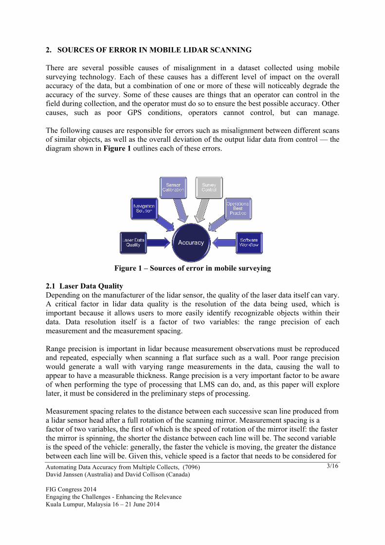
There are several possible causes of misalignment in a dataset collected using mobile surveying technology. Each of these causes has a different level of impact on the overall accuracy of the data, but a combination of one or more of these will noticeably degrade the accuracy of the survey. Some of these causes are things that an operator can control in the field during collection, and the operator must do so to ensure the best possible accuracy. Other causes, such as poor GPS conditions, operators cannot control, but can manage. The following causes are responsible for errors such as misalignment between different scans of similar objects, as well as the overall deviation of the output lidar data from control — the diagram shown in Figure 1 outlines each of these errors.

Figure 1 – Sources of error in mobile surveying

2.1 Laser Data Quality Depending on the manufacturer of the lidar sensor, the quality of the laser data itself can vary. A critical factor in lidar data quality is the resolution of the data being used, which is important because it allows users to more easily identify recognizable objects within their data. Data resolution itself is a factor of two variables: the range precision of each measurement and the measurement spacing. Range precision is important in lidar because measurement observations must be reproduced and repeated, especially when scanning a flat surface such as a wall. Poor range precision would generate a wall with varying range measurements in the data, causing the wall to appear to have a measurable thickness. Range precision is a very important factor to be aware of when performing the type of processing that LMS can do, and, as this paper will explore later, it must be considered in the preliminary steps of processing. Measurement spacing relates to the distance between each successive scan line produced from a lidar sensor head after a full rotation of the scanning mirror. Measurement spacing is a factor of two variables, the first of which is the speed of rotation of the mirror itself: the faster the mirror is spinning, the shorter the distance between each line will be. The second variable is the speed of the vehicle: generally, the faster the vehicle is moving, the greater the distance between each line will be. Given this, vehicle speed is a factor that needs to be considered for


4/16 Automa

laser data quality. Figure 2 below is an image outlining the factors which impact data resolution.

Figure 2 – Data resolution is a factor of range precision & measurement spacing

2.2 INS Errors The most important factor in the absolute spatial accuracy of a survey is the data recorded by the Inertial Navigation System (INS). The reason for this is that the INS data is the source from which vehicle location and orientation are derived, which in turn is used to calculate the XYZ coordinates of all the laser points in a survey. Thus, errors that degrade the quality of navigation solution while collecting data will be forwarded into the laser point calculation. The INS in the Optech Lynx Mobile Mapper™ provided by Applanix is comprised of three components: the IMU, the GPS antennas, and the Distance Measurement Indicator (DMI) (Scherzinger, 2006). All IMUs are subject to inaccuracy in their measurements caused by drift, which can be heightened in conditions like prolonged GPS outages. The DMI is a very important tool for mitigating this error as it provides a redundant method for measuring the distance the vehicle has travelled and aids the IMU in cases of GPS outage. Further discussion about managing these GPS outages to minimize the amount of time the IMU is in Dead Reckoning mode will follow in section 2.3. To minimize error in the orientation measurement of the INS, specifically heading, an operation known as GPS Azimuth Measurement System (GAMS) is performed in which the distance and offset from the primary antenna to the secondary antenna on the vehicle are established. By doing this, the heading accuracy of the INS can be maintained during periods where the vehicle is stationary because there are two independent location readings that


5/16 Automa

maintain a vector between the two antennas, from which a heading value can be established. Other techniques to minimize orientation error include performing dynamic driving prior to a survey to ensure the IMU is properly initialized. After a survey is completed, the operator must correct the observed trajectory with GPS data from a static base station. The baseline distance to this base station does have an impact on the overall accuracy; for example, a baseline distance of 30 kilometers or less is required when collecting data with the Optech’s Lynx Mobile Mapper. The greater the distance to the base station, the less accurate the corrected trajectory will be. 2.3 Operational Best Practices Prior to the collection phase of a project, operators can perform a pre-survey drive to see first-hand the specific environment in which they will be scanning. They can also access online GPS almanacs to choose a time that offers the best possible GPS conditions in the survey location. During the collection phase of the project, following operational best-practice procedures is important for managing the challenging environment that a mobile scan may take place in. The reason for the operational best-practice suggestions is to minimize the amount of error observed from the INS. Optech recommends to all its users that they perform static INS data collection in an area of good GPS conditions at both the commencement and the conclusion of every survey. During periods of prolonged GPS outage during a survey, drift in the IMU results in less accurate location and orientation observations. To manage outages where an IMU is subject to drift (Strus, 2007), the operational best practice is for data collectors to plan their surveys to minimize the amount of time spent surveying in areas of poor GPS. If collection must be performed in an area of poor GPS coverage, the best practice is to find an area with good GPS reception afterward and perform some static data collection there as soon as possible, which will improve the overall accuracy of the survey. The reason for this recommendation is to minimize the amount of time spent in areas of poor GPS and maximize the time spent in those areas of good GPS. By doing this, operators can ensure that the trajectory collected is as good as possible despite the challenging circumstances. For tunnel collects, it is strongly suggested that operators perform static data collection in an open area immediately before entering the tunnel, and again immediately after exiting. The static data collection in this specific situation is useful in aiding the INS, especially the IMU, which will experience a Dead Reckoning environment for an extended period of time in the tunnel. 2.4 Survey Control Depending on the accuracy required from a project, the arrangement of the control network can vary. Typically, prior to an area being scanned, ground control points are distributed throughout the area and their coordinates are established.


6/16 Automa

Projects that need engineering-level accuracy require a greater number of control points collected throughout the project with a total station. For projects that only need mapping-grade accuracy, the control points do not require the same high accuracy and dense distribution. Typically, ground control points collected in the field are clearly identifiable features, either permanent or temporary. A permanent control point might be established on a feature such as a curb, whereas a temporary control point might be a chevron placed adjacent to the drive path in the survey location. During the collection, such a chevron will be observable in the point cloud, allowing adjustments to be made. 3. LIDAR MAPPING SUITE SOLUTION In the mobile lidar manufacturing realm, many advances have been made in hardware. Specifically the pulse repetition frequency (PRF) of the Optech Lynx has gone from the original frequency of 100 kHz to 600 kHz in today’s model. Other hardware changes have included Ladybug® camera integration and an increase in the mirror scanning rate to 250 Hz. However, despite all the hardware advances, the software workflow remained relatively unchanged and has been custom-tailored by mobile lidar users to fit their specific application and business needs. The Optech LMS Lidar Mapping Suite software was designed to allow users to perform rigorous adjustments on their lidar data prior to outputting it into LAS format. The adjustments that can are performed are based upon repeated observations within the data. LMS is capable of various types of adjustments, from minor boresight corrections to more major alignments such as adjusting data to match control points. Finally, LMS offers users many methods of performing quantitative analysis on the dataset prior to outputting the LAS files. These reports include information that offers insight into the quality of the laser data itself, as well as the overall situation as it pertains to the accuracy of the data. 3.1 Laser Point Computation The first step involved in LMS processing is laser point computation (LPC), which involves calculating the XYZ position of each laser point collected during the survey. These coordinates are calculated using the corrected trajectory file and the raw lidar data (containing the angle, range and intensity of each individual laser point) in combination with the calibration information. After the LPC process, LMS has a point cloud that can be used in the later stages of data processing. 3.2 Planar Surface Extraction The second step in LMS processing is to extract planar features from the points calculated during LPC; this is known as planar surface extraction (PSE). There are three factors to consider when extracting planes: plane size, plane width, and surface roughness. Planes must be constrained within a specified minimum and maximum size and must be on a surface flat enough to satisfy the surface roughness variable. If a set is determined to describe a planar


7/16 Automa

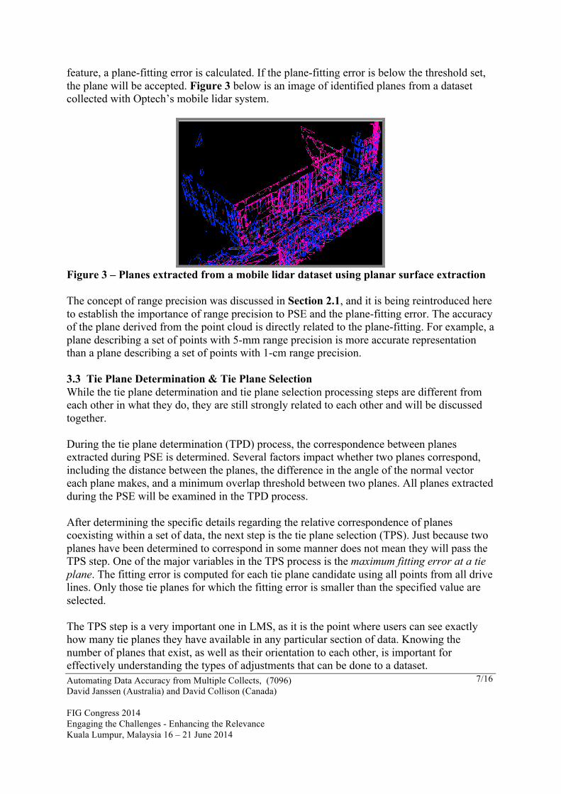
feature, a plane-fitting error is calculated. If the plane-fitting error is below the threshold set, the plane will be accepted. Figure 3 below is an image of identified planes from a dataset collected with Optech’s mobile lidar system.

Figure 3 – Planes extracted from a mobile lidar dataset using planar surface extraction The concept of range precision was discussed in Section 2.1, and it is being reintroduced here to establish the importance of range precision to PSE and the plane-fitting error. The accuracy of the plane derived from the point cloud is directly related to the plane-fitting. For example, a plane describing a set of points with 5-mm range precision is more accurate representation than a plane describing a set of points with 1-cm range precision. 3.3 Tie Plane Determination & Tie Plane Selection While the tie plane determination and tie plane selection processing steps are different from each other in what they do, they are still strongly related to each other and will be discussed together. During the tie plane determination (TPD) process, the correspondence between planes extracted during PSE is determined. Several factors impact whether two planes correspond, including the distance between the planes, the difference in the angle of the normal vector each plane makes, and a minimum overlap threshold between two planes. All planes extracted during the PSE will be examined in the TPD process. After determining the specific details regarding the relative correspondence of planes coexisting within a set of data, the next step is the tie plane selection (TPS). Just because two planes have been determined to correspond in some manner does not mean they will pass the TPS step. One of the major variables in the TPS process is the maximum fitting error at a tie plane. The fitting error is computed for each tie plane candidate using all points from all drive lines. Only those tie planes for which the fitting error is smaller than the specified value are selected. The TPS step is a very important one in LMS, as it is the point where users can see exactly how many tie planes they have available in any particular section of data. Knowing the number of planes that exist, as well as their orientation to each other, is important for effectively understanding the types of adjustments that can be done to a dataset.


8/16 Automa

The concept of point-to-plane distance analysis, whose graphical analysis is below in Figure 4, is fundamental to processing in LMS.

Figure 4 – Point-to-plane analysis

For each laser point that lies on a tie plane (that is, a plane that is covered by more than one drive line), the vertical distance ds to the plane can be computed. In the absence of system errors, these distances are partly a function of random errors (noise) of in the laser points and partly a function of the surface roughness. If systematic errors are present, they also show up in these distances. Therefore, the point-to-plane distance ds can be used for assessing the quality of the laser point cloud. 3.4 Self-Calibration At this stage, the laser points have been calculated (LPC), the planes within the data have been extracted (PSE), the correspondence between the planes has been determined (TPD) and that correspondence has been confirmed to meet a defined threshold (TPS). From the planes that passed the TPS, a least-squares adjustment will be performed on all of the planes present within a dataset to minimize the weighted square sum of observable residuals and determine the set of parameters that require modification to realize this least-squares adjustment. There are three parameters that can be adjusted when performing the self-calibration: boresight, position and orientation. Within each of these three options the user can customize which parameters they would like to adjust (free unknown) and which they would like to remain unchanged (keep fixed). Users are also able to keep some parameters fixed, but within a prescribed limit (constrain unknown). For boresight parameters, users can set the boresight angle roll to free unknown so as to calculate the optimal roll value for a specific drive line. Similar adjustments can be performed with other boresight parameters, such as pitch and heading. Lever arm values can also be optimized for a particular survey or drive line in a survey.


9/16 Automa

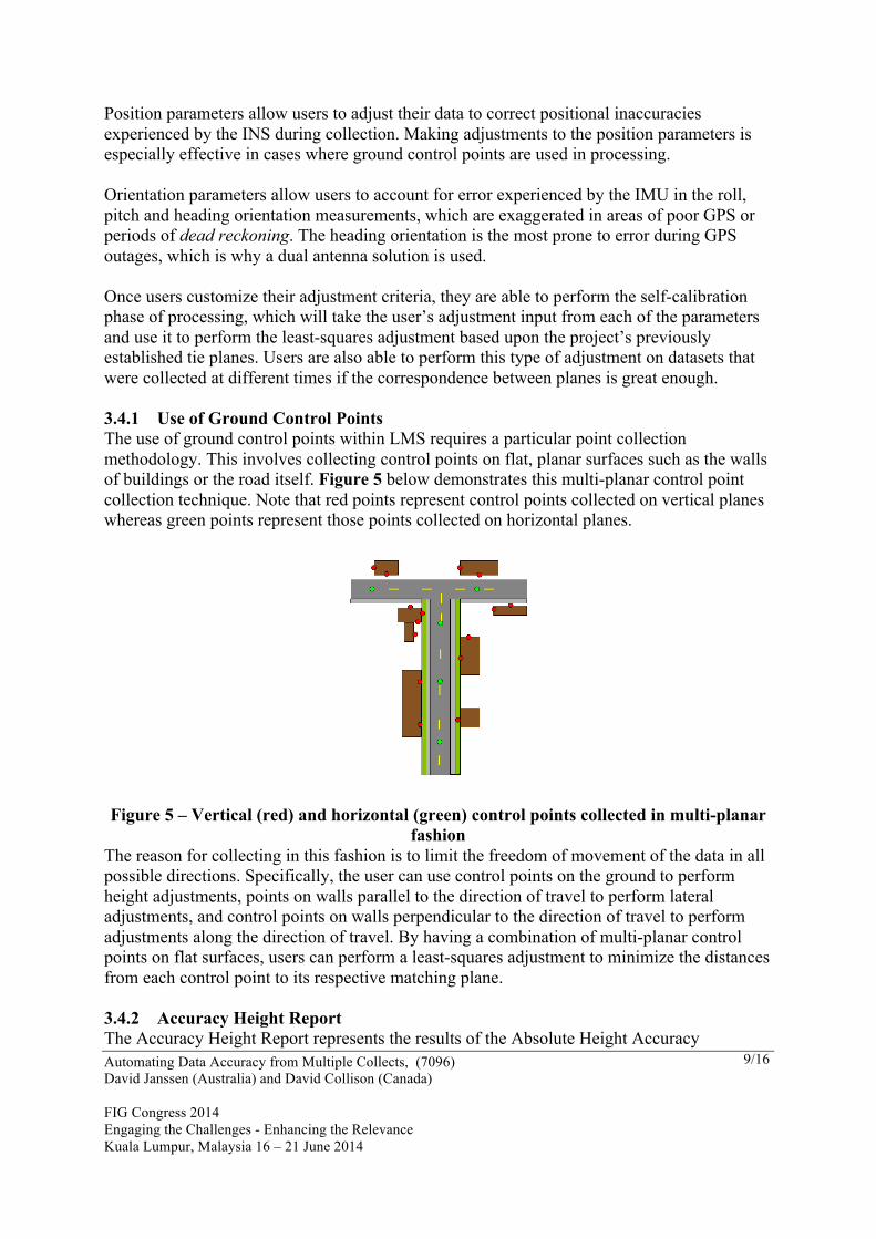
Position parameters allow users to adjust their data to correct positional inaccuracies experienced by the INS during collection. Making adjustments to the position parameters is especially effective in cases where ground control points are used in processing. Orientation parameters allow users to account for error experienced by the IMU in the roll, pitch and heading orientation measurements, which are exaggerated in areas of poor GPS or periods of dead reckoning. The heading orientation is the most prone to error during GPS outages, which is why a dual antenna solution is used. Once users customize their adjustment criteria, they are able to perform the self-calibration phase of processing, which will take the user’s adjustment input from each of the parameters and use it to perform the least-squares adjustment based upon the project’s previously established tie planes. Users are also able to perform this type of adjustment on datasets that were collected at different times if the correspondence between planes is great enough. 3.4.1 Use of Ground Control Points The use of ground control points within LMS requires a particular point collection methodology. This involves collecting control points on flat, planar surfaces such as the walls of buildings or the road itself. Figure 5 below demonstrates this multi-planar control point collection technique. Note that red points represent control points collected on vertical planes whereas green points represent those points collected on horizontal planes.

Figure 5 – Vertical (red) and horizontal (green) control points collected in multi-planar fashion

The reason for collecting in this fashion is to limit the freedom of movement of the data in all possible directions. Specifically, the user can use control points on the ground to perform height adjustments, points on walls parallel to the direction of travel to perform lateral adjustments, and control points on walls perpendicular to the direction of travel to perform adjustments along the direction of travel. By having a combination of multi-planar control points on flat surfaces, users can perform a least-squares adjustment to minimize the distances from each control point to its respective matching plane. 3.4.2 Accuracy Height Report The Accuracy Height Report represents the results of the Absolute Height Accuracy


10/16

algorithm. This algorithm calculates the height difference (offset) for all control points with respect to the surrounding laser points and produces statistics regarding these changes. The Accuracy Height Report contains the height difference (offset) for each control point, as well as the average height difference and standard deviation calculated before and after the adjustment. Only those control points specified on horizontal planes are used in the Accuracy Height Report. 4. CASE STUDY IN BRITISH COLUMBIA, CANADA In May 2013 Optech travelled to Vernon, British Columbia to perform a data collection and used LMS in the processing of the data. The collection was done to demonstrate mobile surveying technology to the local transportation authorities as a feasibility study for their specific use as it pertained to road monitoring and maintenance. Due to challenges with intermittent rain, the first half of the collection took place May 21, and the second portion was collected on May 23. However, some portions of the region of interest were collected on both days, and this case study will examine the data from those portions. Figure 6 below is a Google Earth image of the trajectories collected on each respective day during the collection.

Figure 6 – Collection of an intersection in Vernon, BC

On May 21, 2013 the survey lasted for 1 hour and 53 minutes, covering a total distance of 77.8 kilometers. The survey commenced in Kelowna and proceeded north along Highway 97 north of Vernon, passing through the city centre en route. On May 23, 2013 the survey lasted for 1 hour and 14 minutes, covering a total distance of 46.9 kilometers. This survey followed a very similar route north out of Kelowna on Highway

May 21 May 23


11/16

97, but in this survey an intersection was scanned multiple times as demonstrated in Figure 6 above. The equipment used for the collection was an Optech Lynx Mobile Mapper™, specifically an M1 model containing two sensor heads, each capable of collection rates of 500 kHz and mirror scanning speeds of 200 Hz. It also had four 5-MP cameras and used an FMU P300 IMU in its INS. The equipment was ferried up to the project site from Vancouver where it had been left after a previous demonstration. 5. CASE STUDY RESULTS The point-to-plane analysis is performed on the dataset both before and after the self-calibration step in LMS, and thus users are able to see the overall spatial variation of the planes in their data before and after the least-squares adjustment has taken place. Figure 7 below is an image of the summary plot from the qualitative report generation of LMS, representing the accuracy analysis at all tie planes from standard processing (that is, processing that occurred prior to the least-squares adjustment).

Figure 7 – Accuracy analysis at all tie planes from standard processing

The x-axis in the graph represents the optical scan angle of the laser beam as it left the scanning window of the sensor head and the y-axis represents the average point-to-plane distance per plane and drive line. The two types of tie planes being analyzed in this graph are those with plane slopes ≤2.0° (represented by red points in the graph) and those with plane slopes >2.0° (represented by blue points). What is noticeable about this graph is the increase in the average point-to-plane distance at +90° and -90°, specifically in the slopes > 2.0°. This is representative of the planar separation between vertical walls, which is caused by the sources of error in mobile lidar scanning discussed in Section 2. Seen below, Figure 8 represents the histogram of the point-to-plane distances per plane and drive line. It is not separated by planar orientation like the scatterplot in Figure 7, but like the scatterplot there is large variation visible in the data’s deviation about the mean.


12/16

Figure 8 – Accuracy analysis at all tie planes from standard processing

After the adjustments to the data were performed, we were able to analyze the same plots again to observe the changes in the average point-to-plane distances. By comparing Figure 9 below with Figure 7 above, we observed a noticeable decreasing value of the average point-to-plane distance, especially for those planes collected at -90° and +90°.

Figure 9– Accuracy analysis at all tie planes from refined processing

Seen below, Figure 10 represents the histogram of the point-to-plane distances per plane and drive line. Similar to the noticeable decrease in the average point-to-plane distances from Figure 9, the histogram demonstrates a noticeable increase in the frequency of data about the mean.


13/16

Figure 10 – Accuracy analysis at all tie planes from refined processing

For this particular project, control points were provided for ground points only, not on vertical planar features such as walls of buildings. Therefore, as discussed in Section 3.4.1, only vertical adjustments to the data are represented in Figure 11 below.

Figure 11 – Height offset plot

In total there were 957 points used for this vertical adjustment of the data. In standard processing, the average height distance was 0.019 meters and the standard deviation was 0.029. After the adjustment had taken place, the average height distance was -0.004 meters and the standard deviation was 0.031. Below, Table 1 outlines the adjustments that were made to each respective boresight, position and orientation parameter in this particular project. In each case it was selected that the changes were only applied to each mission.


14/16

Table 1: Boresight, position & orientation corrections

For boresight corrections, there were two sets of corrections to each of the two sensors, and therefore four records of adjustments. Positional corrections were made for each individual survey (hence the two different sets of positional adjustments) and orientation parameters were made on a line-by-line basis regardless of which survey the line belonged to. There were 52 lines in this particular data adjustment, and 20 of the adjustment values are represented in Table 1. 6. CONCLUSION There are multiple sources of error present throughout the process of collecting and later processing mobile lidar data that everyone must contend with in order to make a project successful. In addition to understanding where each of these sources of error come from, users must also have a sound understanding of the severity of the consequences these errors have on their data, and the steps required to correct these inaccuracies.


15/16

Through the extraction of planar surfaces found within the processed lidar data itself and the establishment of their relative spatial correspondence, LMS is capable of identifying and quantifying these errors, through which it can then make adjustments to the overall accuracy of the data. In the case study explored in this paper, surveys from different times were combined for processing together to demonstrate how this planar extraction can be used in an automated fashion to improve the overall relative and absolute accuracy of a mobile survey even in cases where the collect was done on different days. REFERENCES Scherzinger, B & Hutton, Joe. Applanix IN-Fusion Technology Explained. 2006. http://www.applanix.com/media/downloads/articles_papers/Applanix%20IN-Fusion.pdf Strus et al. Development of High Accuracy Pointing Systems for Maneuvering Platforms. ION GNSS 20th International Technical Meeting of the Satellite Division. 2007. http://www.beidoudb.com:88/document/uploads/e1583852-fd16-4175-940d-5b0f91b27852.pdf BIOGRAPHICAL NOTES David Janssen studied Geography at Wilfrid Laurier University in Waterloo, Canada, graduating in 2007. In August 2008, David was a graduate of Sir Sanford Fleming College (Frost Campus) in Lindsay, Canada with a Geographic Information Systems Application Studies certificate. Since 2010, David has worked at Optech Incorporated, starting in a support role for Optech’s hardware. In 2013, David transitioned to his current position of Product & Application Specialist for Mobile Products. The author would like to acknowledge Thomas Montour of Optech for aiding in the creation of figures within the article. CONTACTS Mr. David Janssen Optech Incorporated 300 Interchange Way Vaughan, ON


16/16

CANADA Tel. +1 (905) 660-0808 Fax + 1 (905) 660-0829 Email: [email protected] Web site: www.optech.com

automating data accuracy from multiple collects - fig · automating data accuracy from multiple...

Documents