Automating Judgement and Decisionmaking:Theory and Evidence from Resume Screening

Bo Cowgill∗Columbia University

May 5, 2017

Preliminary and incomplete. Do not circulate.

Abstract

What types of decisionmaking tasks are better automated? And which are better left tojudgement? I develop a formal model of the comparative advantages of human judgementand machines in decisionmaking. I subsequently test these predictions in a field experimentin applying machine learning for hiring workers for white-collar team-production jobs. Themarginal candidate picked by the machine (but not by human screeners) is +17% more likelyto pass a face-to-face interview with incumbent workers and receive a job offer offer, b) +15%more likely to accept job offers when extended by the employer and c) 0.2σ-0.4σ more produc-tive once hired as employees. Consistent with the model, the algorithm’s advantage comes inselecting candidates from high variance applicant pools, such as candidates who lack job re-ferrals, those without prior experience, those with atypical credentials and those completing aPhD. I also find that machine candidates are +12% less likely to show evidence of competing joboffers during salary negotiations. I also find that algorithmic judgment results in better perfor-mance in abstract, hard-to-measure dimensions of candidates – such as leadership, cultural fitand other non-cognitive “soft” dimensions – which is a prediction of the model. I conclude bydiscussing the implications of machine learning for a variety of decisionmaking tasks through-out the economy.

∗The author thanks seminar participants at the 2015 Empirical Management Conference, the Institutions and In-novation Conference at Harvard Business School, the Tinbergen Institute, Universidad Carlos III de Madrid, NBEREconomics of Digitization, the Kauffman Emerging Scholars Conference, Columbia Business School, the Center forAdvanced Study in the Behavioral Sciences (CASBS) at Stanford, the Summer Institute for Competitive Strategy atBerkeley, the Wharton People and Organizations Conference, NBER Summer Institute (Labor), the NYU/Stern Cre-ativity and Innovation Seminar and the University of Chicago Advances in Field Experiments Conference, as well asJason Abaluck, Ajay Agrawal, Susan Athey, Thomas Barrios, Laura Gee, Dan Gross, John Horton, Danielle Li, ChristosMakridis, Stephan Meier, John Morgan, Harikesh Nair, Paul Oyer, Tim Simcoe and Jann Spiess.

1

1 Introduction

Social skills and other soft skills are increasingly rewarded in the labor market. Deming (2015) andWeinberger (2014) provides compelling evidence that in the past 40 years, employment and wagegrowth has been strongest in jobs that require both cognitive skill and social skill. Deming (2015)shows that nearly all job growth in the US since 1980 has been in occupations intensive in socialskills.

One reason for this increase is that social interactions and cultural understanding requires sub-tle, tacit knowledge that cannot be easily automated (Autor, 2015). Thus workers bearing theseskills cannot be easily displaced by machines. Economists in this literature cite evolutionary the-orists (Moravec, 1988) who argue that social interaction is an unconscious process that evolvedover thousands of years – thus cannot be easily replicated by robots. In this sprit, Frey and Os-borne (2013) identify social intelligence tasks as a key bottleneck to further automation. Armed withthis reasoning, economists, policymakers and education reformeres have proposed curriculumchanges, suggesting that tomorrow’s students should learn social skills to protect their employa-bility against technological innovation.

Are human social skills truly so productive and resistant to automation? The answer may affectthe future returns to soft skills. Many of the widespread shortcomings documented in behavioraleconomics – attribution errors, homophily bias and others – are shortcomings in social judgements.In other contexts, the evolutionary origins of human behavior were irrelevant to automation1 orpresent clear disadvantages.2 Algorithms have been often suggested as a way to improve uponflawed human decision-making (Kahneman, 2011), not to coarsen it.

Do humans truly have better social skills?3 The idea might be a seductive illusion kept alive bymeasurement challenges. Counterfactual social judgements are rarely observed. Even when theyare, scoring and evaluating outcomes may be subjective, noisy or require years to realize.4 The

1For example, many scholars belive that facial recognition is a subconscious process that required thousands of yearsto evolve (Parr, 2011). However, modern facial recognition software is capable of outperforming humans at labelingsimilar faces (Taigman et al., 2014; Schroff et al., 2015).

2For example, in dieting.3A popular of evidence about automating social interactions is the failure of progress on the “Turing Test.” The

Turing Test is a laboratory game in which a human judge converses via text with an anonymous agent. After an un-structured text conversation, the judge must guess if the agent is a person or a computer program. A computer program“passes” if it successfully fools the judge into labeling it a human, which is difficult for machines to accomplish. Thejudge’s Type II errors are rarely disclosed or discussed.

There are many reasons to be skeptical of the generalizability of this laboratory result. Some computer programssucceed by deliberately adopting common human errors, rather than emulating the productivity and utility of humanjudgement. See LaCurts (2011) for a discussion of the limits of Turing Test results.

Notably: In real-world settings – where firms face non-laboratory incentives to distinguish robots from humans –businesses rely on machine judges, not human judges. For example: Unwanted computer-generated email costs Amer-icans over $20 billion annually and generates $200M in revenues for spam companies (Rao and Reiley, 2012). The jobof separating computer-generated emails from “genuine” human-generated messages is a real-world “Turing Test.”Real-world firms in this business delegate the task to algorithms, not humans.

4In many settings, agents may actively obfuscate how social outcomes are scored. In some circumstances, good socialskills by one party may require ignoring or mislabeling one’s own (or someone else’s) previous bad social decisions. Forexample: Holiday gift-giving is an activity requiring social skills but that may result in mismatch (Waldfogel, 1993).Nonetheless, recipients of undervalued gifts often report happiness with the chosen gift, thus obfuscate scoring of thegift choice. Similarly: A boss may attempt to divert attention from bad hiring decisions in order to avoid embarrassment,

2

unit of analysis may not be clear: This literature often stresses “interactiveness,” in which manysocial decisions are bundled together. The measurement issues around social skills also createsmoral hazard in contracting. If identifying a job candidate’s “cultural fit” cannot easily be verified,workers can exploit ambiguity for private gain. For example, a hiring manager may feign “culturalfit” as cover for employing cronies, relatives or favorites instead of a better-suited worker.

The features that make social interactions difficult to automate also make these tasks difficult tomeasure and contract upon.5 By contrast, differences in hard skills (such as mathematics) may bemuch easier to both measure and contract upon.6 These measurement and contracting differences– and not underlying technological performance differences – may be why we believe that hardskills can be effectively automated while soft skills cannot.

This paper examines these questions experimentally in the setting of hiring for team-based,white-collar jobs. Hiring decisions in this environment are intimately linked to social interactionand compatibility. In many industries, new employees often first must learn and be mentored byincumbent employees, and then later interact and collaborate with other workers in order to createvalue. A recent survey of ≈3,000 hiring managers, 43% listed “cultural fit” as the “single most im-portant determining factor when making a new hire.”7 The importance of social relationships andcompatibility are one reason that many firms tap into pre-existing social relationships (see Burkset al., 2015) in hiring decisions.

Deming (2015) writes that effective social skills require “the capacity that psychologists call the-ory of mind - the ability to attribute mental states to others based on their behavior, or more col-loquially to ‘put oneself into anothers shoes’ (Premack and Woodruff, 1978; Baron-Cohen, 2000;Camerer et al., 2005)” or “[r]eading the minds of others.”

By this definition of social skills, hiring managers must not only read the candidate’s mind, butalso read the minds of interviewers, co-workers, managers and clients who may interact with thecandidate in the future. Screeners involved in hiring must make inferences about soft skills basedon social signals in letters of reference, interviews and CVs. Efficient hiring requires selectingcandidates likely to pass job interviews – face-to-face exchanges with incumbent workers in whichsubconscious and subtle non-verbal communication influence outcomes – and who are likely tocooperate productively with future teammates in on-the-job work.

Hiring decisions have attractive measurement properties: In this setting, the exercise of socialperceptiveness involve discrete decisions with a natural unit of analysis: For a given candidate,should he or she be interviewed? This discreteness is distinct from the many bundled decisions ofreal-time conversations. The use of a field experiment enables researchers to observe counterfac-

avoid disruptive firings and/or focus attention how to best utilize the strengths of the hired worker. This may compelthe boss to misrepresent the employee’s quality – or to compensate by providing extra coaching and tutoring for thefailed candidate. In both cases, social pressures require agents to confound measurement and obfuscate how outcomesare scored.

5A related contracting issue is: When outcomes take a long time to be realized – as is the case in hiring and manyother tasks requiring social skills – it may be difficult to incentivize present-biased agents.

6There is often a single right answer and a single, provably optimal method for arriving at this answer; as such thereis less subjectivity in scoring outcomes. The timeliness of measuring hard skills is easier. Computers derive much oftheir benefit from fast computation, and human subjects may quickly realize when they are stumped (hastening thetime necessary to measure and compare outcomes).

7http://about.beyond.com/press/releases/20140520-National-Survey-Finds-College-Doesnt-Prepare-

Students-for-Job-Search

3

tual outcomes and observe differences. How does a human and machine screener assess the sameset of candidates? How often does the human and algorithm disagree? Who is more “correct” inthese disagreements – particularly on dimensions of performance relating to “soft” skills such ascultural fit, leadership and social interaction?

To understand these issues, I develop a model of automating subjective judgements. In themodel, a mass of human agents face a series of binary decisions. Each has a taste-based preferencewhich is hidden from the principal. Each agent also has a statistical model of the the “correct”decision, but can only be compeled via contracting to make that decision regularly. Contractingmay fail for two reasons: First, because outcomes are hard to verify which weakens incentives.Second, because the agents’ statistical models are rudimentary and update slowly.

I then compare the performance of this mass of humans against machine learning trained onhistorical data by the mass of human agents. The machine learning effectively integrates overeach human individuals’ idiosyncratic tastes, canceling out much (but not necessarily all) of thebiases of the human processes. The algorithm’s advantage thus comes from three sources: First,canceling out idiosyncratic biases. Second, attending to more variables and thus having a betterstatistical model, and third: Because the algorithm can pool information from the entire mass ofhumans, it can update its model and can learn more quickly. The algorithm is effectively a form oforganizational centralization with superior coordination – in the form of learning – between agents(Alonso et al., 2008).

I then examine the results of a field experiment motivated by this model. The field experimentyields four main results.

First, the machine and human screeners disagree on about 30% of candidates. I find that themarginal candidate picked by the machine (but not by the human) is +17% more likely to passa double-blind face-to-face interview with incumbent workers and receive a job offer offer. Themarginal candidate picked by a human (but not the machine) is less likely to pass the double-blindinterview. I show evidence that the machine candidates pass the interview panel in part becausetheir worst (most negative) interview evaluation from the panel are more favorable. By contrast,the most positive evaluations from the panel are roughly similar to the human-picked candidates.The algorithm benefits candidates coming from an atypical career or educational backgrounds (forexample, a school not attended by any other applicant in the firm’s applicant pool).

Second, I find that are also more likely to accept job offers conditional on being extended. Theyare also about 12% less likely to show evidence of competing job offers during salary negotiations,and are 15% more likely to accept job offers when extended by the employer.

Third, these are about 0.2σ-0.4σ more productive once hired as employees.

Lastly, evaluations of the candidates shows that advantage of the machine comes from select-ing candidates with superior soft skills such as leadership and cultural fit, and not from findingcandidates with better cognitive skills. The computer’s advantage appear precisely the soft di-mensions of employee performance which prior literature suggests humans – and not machines –have innately superior judgement.

I also find that tests of combining human and algorithmic judgement fare poorly for human judge-ment. Regressions of interview performance and job acceptance on both human and machine as-

4

sessments puts most weight on the machine signal.

While this setting has inherent limitations, these results show evidence of productivity gainsfrom IT adoption in tasks requiring social judgements. Limiting or eliminating human discretionthrough this form of digitization improves both the rate of false positives (candidates selectedfor interviews who fail) as well as false negatives (candidates who were denied an interview, butwould have passed if selected). These benefits come exclusively through re-weighting informationon the resume – not by introducing new information (such as human-designed job-tests or surveyquestions) or by constraining the message space for representing candidates.

Section 2 discusses the empirical setting and experimental design, and in section Section 4 Isummarize results. Section ?? concludes with discussion of some reasons labor markets may re-ward “soft skills” even if they can be effectively automated, and the effect of integrating machinelearning into production processes.

2 Empirical Setting

The job openings in this paper are technical staff such as programmers, hardware engineers andsoftware-oriented technical scientists and specialists. Workers in this industry are involved inmulti-person teams that design and implement technical products.

Successful contributions in this environment requires workers to collaborate with colleagues. Ina typical project, a new product can be conceptualized as several interacting technical “modules”that function together as a coherent product. Each team member is tasked with designing andimplementing a module, and ensuring that the technology of his or her module cooperates withothers’. The team discusses as a group to achieve consensus on the macro-level segmentation ofthe product into “modules” and the assignment of various modules to teammates. Frequentlycircumstances arise that require these workers to switch module assignments. For example, somemodules may take unexpectedly long and need to be subdivided. This resembles Deming’s 2015“trading tasks.”

The internal promotion process in this market often involves peer feedback and subjective per-formance reviews. In fact, the incentives for positive subjective reviews from workplace peersare so strong that a number of scholars and journalists have expressed concern that these sys-tems encourage “influence activities” (Milgrom and Roberts, 1988; Milgrom, 1988, Gubler et al.,2013) – that is, the system encourages social skills rather than programming. Eichenwald’s 2012journalistic account of Microsoft’s promotion system8 says that “[E]very employee has to impressnot only his or her boss but bosses from other teams as well. And that means schmoozing andbrown-nosing as many supervisors as possible.”

Work in this industry thus involves substantial amounts of coordination, negotiation, persuasionand social perceptiveness – which the four skills in the the O*NET database in used by Deming(2015) to label jobs requiring social skills. This is especially true if one considers the behaviorsnecessary to be promoted. Consistent with this account, the occupations corresponding to this

8 http://www.vanityfair.com/business/2012/08/microsoft-lost-mojo-steve-ballmer

5

work rank above the median in the O*NET database.9

Separately from the underlying job details, the hiring process itself in white-collar work often re-quires substantial coordination, negotiation, persuasiveness and social perception. Job candidatesare often evaluated by a panel of interviewers who have differing needs and opinions, and whosefeelings must be distilled into actionable decisions. For example: While a firm may be hiring fora role in one division, they may find another candidate who is better-matched for in a relateddivision. Who has prioritized access to the candidate? Can a new position be created that com-bines both divisions? If so, what is the career path in this hybrid position, and what happens tothe previous openings – does the hybrid job replace either or both earlier requisitions? Settlingthese questions may require discussion, persuasion and trading favors between divisions and/ormembers of the hiring panel.

In making an interviewing decision, a screener must put himself or herself into all of the shoesof many potentially affected parties – both those involved in the final job placement, as well asthose involved in the hiring process. In addition, the screener must put himself or herself in themind of the candidate: Will the candidate already have another job offer that he/she will likemore? Will the candidate want the job after learning more details? How will the candidate react topeculiarities of pay, coworkers and procedures?

For these reasons, the O*NET occupation “human resource specialists” also ranks highly on allfour O*NET measures of social skills (coordination, negotiation, persuasion and social perceptive-ness). The actions automated in this paper are the decisions to to interview (or reject) candidates.This is only one part of the full hiring process. However, the initial decision is tied to the later out-comes through incentives: In this industry, HR specialists are awarded substantial performanceincentives for selecting a candidate who passes screening. For this reason, the screeners (and theirautomated replacements) must be able to anticipate the social aspects of later screening and per-formance outcomes.

A few details inform the econometric specifications in this experiment. In this talent market,firms commonly desire as many qualified workers as it can recruit. Firms often do not have aquota of openings for these roles; insofar as they do they are never filled. “Talent shortage” is acommon complaint by employers regarding workers with technical skills. The economic problemof the firms is to identify and select well-matched candidates, and not to select the best candidatesfor a limited set of openings. Applicants are thus not competing against each other, but against thehiring criteria.

The application process for jobs in this market proceeds as follows. First, candidates apply to thecompany through a website.10 Next, a human screener reviews the applications of the candidate.This paper includes a field experiment in replacing these decisions with an algorithm.

9The exact categorization of these jobs in the O*NET database requires some interpretation. Based on title alone, themost similar occupation is “Software Developers, Applications.” On these four measure, is at the median for three andslightly below for the fourth (social perceptiveness). However, the job description in O*NET for this occupation leavesout the design and coordination aspects of the job. These aspects are better captured in the occupations labeled “Com-puter and Information Systems Managers” and “Information Technology Project Managers,” both of which rate highlyon all four measures of social skills. Like the jobs in this paper, the “management” expressed in these latter O*NET occu-pations does not necessarily involve direct command authority over subordinates and often refer to managing processesthrough coordination.

10Some candidates are also recruited or solicited; the applications in this study are only the unsolicited ones.

6

The next stage of screening is bilateral interviews with a subset of the firm’s incumbent workers.The first interview often takes place over the phone. If this interview is successful, a series of in-person interviews are scheduled with incumbent workers, lasting about an hour. The interviewsin this industry are mostly unstructured, with the interviewer deciding his or her own questions.Firms offer some guidance about interview content but don’t strictly regulate the interview content(for example, by giving interviewers a script).

After the meetings, the employees who met the candidate communicate the content of the in-terview discussion, impressions and a recommendation. During the course of this experiment,the firm also asked interviewers to complete a survey about the candidate evaluating his or hergeneral aptitute, cultural fit and leadership ability. With the input from this group, the employerdecides to make an offer.

Next, the candidate can then negotiate terms of the offer not. Typically, employers in this marketengages in negotiation only in order to respond to competing job offers. The candidate eventuallyaccepts or rejects the offer. Those who accept the offer begin working. At any time the candidatecould withdraw his application if he or she accepts a job elsewhere or declines further interest.

The setting from this study is a single firm with several products and services. The sample inthis paper is only for one job opening, and for one geographic location where there is an office.11

The hiring company does not decline to pursue applications of qualified candidates on the beliefthat certain candidates “would never come here [even if we liked him/her].” For these jobs, theemployer in this paper believes it can offer reasonably competitive terms; it does not terminateapplications unless a) the candidate fails some aspect of screening, or b) the candidate withdrawsinterest.

For the analysis in this paper, I code an applicant as being interviewed if he/she passed theresume screen and was interviewed in any way (including the phone interview). I code candidatesas passing the interview if they were subsequently extended a job offer.

Table 1 contains descriptive statistics and average success rates at the critical stages above. Asdescribed in the next section, the firm used a machine learning algorithm to rank candidates. Table1 reports separate results for the “Top 1%-2%” – the subjects of the experiment in this study – andthe remainder of applicants.

Table 1 shows that the candidates above the machine’s threshold are positively selected on anumber of traits. They also tend to pass rounds of screening at much higher rates even withoutany intervention from the machine. One notable exception is the offer acceptance rate, which islower for the candidate that the machine ranks highly. One possible explanation for this is that thealgorithms’ model is similar to the broader market’s, and highly ranked candidates may attractcompetitive offers.

2.1 Selection Algorithm

Firms offering products and consulting in HR analytics have exploded in recent years, as a resultof several trends. On the supply side of applications, several factors have caused an increase in

11In this industry, candidates are typically aware of the geographic requirements upon applying.

7

application volumes for posted jobs throughout the economy. First, the digitization of job appli-cations has lowered the marginal cost of applying. Second, the Great Recession caused a greaternumber of applicants to be looking for work. On the demand side, recent information technol-ogy improvements have enabled firms to handle the volume of online applications. Firms aremotivated to adopt these algorithms in part of the volume/costs, and also because of the addresspotential mistakes in the judgements of human screeners.

How common is the use of algorithms for screening? The public appears to believe it is alreadyvery common. The author conducted a survey of≈3,000 US Internet users, asking “Do you believethat most large corporations in the US use computer algorithms to sort through job applications?”12

About two-thirds (67.5%) answered “yes.”13 Younger and more wealthy respondents were morelikely to answer affirmatively, as were those in urban and suburban areas.

A 2012 Wall Street Journal article14 estimates that the proportion of large companies using resume-filtering technology as “in the high 90% range,” and claims “it would be very rare to find a Fortune500 company without [this technology].”15 The coverage of this technology is sometimes negative.The aforementioned WSJ article suggests that someone applying for a statistician job could be re-jected for using the term “numeric modeler” (rather than statistician). However, the counterfactualhuman decisions mostly left unstudied. Recruiters’ attention is necessarily limited, and humanscreeners are also capable of mistakes which may be more egregious than the above example. Onecontribution of this paper is to use exogenous variation to observe counterfactual outcomes.

The technology in this paper uses standard text-mining and machine learning techniques thatare common in this industry. The first step of the process is broadly described in a 2011 LifeHackerarticle16 about resume-filtering technology:17 “[First, y]our resume is run through a parser, whichremoves the styling from the resume and breaks the text down into recognized words or phrases.[Second, t]he parser then sorts that content into different categories: Education, contact info, skills,and work experience.”

In this setting, the predictor variables fall into four types.18 The first set of covariates was aboutthe candidate’s education such as institutions, degrees, majors, awards and GPAs. The secondset of covariates is about work experience including former employers and job titles. The thirdcontains self-reported skill keywords that appear in the resume.

The final set of covariates were about the other keywords used in in the resume text. The key-words on the resumes were first merged together based on common linguistic stems (for example,“swimmer” and “swimming” were counted towards the “swim” stem). Then, resume covariates

12The phrasing of this question may include both “pure” algorithmic screening techniques such as the one studied inthis paper, as well as “hybrid” methods, where a human designs a multiple-choice survey instrument, and responsesare weighted and aggregated by formula. An example of the latter is studied in Hoffman, Kahn and Li (2016).

13Responses were reweighed to match the demographics of the American Community Survey. Without the reweigh-ing, 65% answered yes.

14http://www.wsj.com/articles/SB10001424052970204624204577178941034941330, accessed June 16, 2016.15As with the earlier survey, this may include technological applications that differen than the one in this paper.16http://lifehacker.com/5866630/how-can-i-make-sure-my-resume-gets-past-resume-robots-and-into-

a-humans-hand17Within economics, this approach to codifying text is similar to Gentzkow and Shapiro (2010)’s codification of polit-

ical speech.18Demographic data are generally not included in these models and neither are names.

8

were created to represent how many times each stem was used on each resume.19

Although many of these keywords do not directly describe an educational or career accomplish-ment, they nonetheless have some predictive power over outcomes. For example: Resumes oftenuse adjectives and verbs to describe the candidate’s experience in ways that may indicate his or hercultural fit or leadership style. For example: Verbs such as “served” and “directed” may indicatedistinct leadership styles that may fit into some companies’ better than others. Such verbs wouldbe represented in the linguistic covariates – each resume would be coded by the number of timesit used “serve” and “direct” (along with any other word appearing in the training corpus). If themachine learning algorithm discovered a correlation between one of these words and outcomes, itwould be kept in the model.

For each resume, there were millions of such linguistic variables. Most were excluded by thevariable selection process described below. The training data for this algorithm contained histor-ical resumes from previous four years of applications for this position. The final training datadataset contained over one million explanatory variables per job application and several hundredthousand successful (and unsuccessful) job applications.

The algorithms used in this experiment machine learning methods – in particular, LASSO (Tib-shirani, 1996) and support vector machines (Vapnik, 1979; Cortes and Vapnik, 1995) – to weighcovariates in order to predict success of the historical applications for this position. Applicationswere coded as successful if the candidate was extended an offer. A standard set of machine learn-ing techniques – regularization, cross-validation, separating training and test data – were used toselect and weigh variables.20 These techniques (and others) were ment to ensure that the weightswere not overfit to the training data, and that the algorithm accurately predicted which candidateswould succeed in new, non-training samples.

A few observations about the algorithm. First, the algorithm introduced no new data into thedecision-making process. In theory, all of the covariates described above can also be observedby human resume screeners. The human screeners could also view an extensive list of historicaloutcomes on candidates. In a sense, any comparisons between humans and this algorithm is in-herently unfair to the machine. A human can quickly consult the Internet or a friend’s advice toexamine an unknown’ school’s reputation. The algorithm was given no method to consult outsidesources or bring in new information that the human couldn’t.

Second: This modeling approach imposes no constraints on the job applicant’s message space.The candidate can fill the content of her resume with whatever words she chooses. The candi-date’s experience was unchanged by the algorithm and his/her actions were not required to bedifferent than the status quo human process. As with a spoken conversation with a hiring man-ager, this algorithm did not impose constraints on what mix of information, persuasion, framingand presentation a candidate could use in her presentation of self.

By contrast, other “automated” job screening interventions drastically limit the candidate’s mes-sage space. For example, the variables introduced in the screening algoritm studied by Hoffman,Kahn and Li (2016) are responses to human-designed, multiple-choice survey instrument which

19The same procedure was used for two-word phrases on the resumes.20See Friedman et al. (2013) for a comprehensive overview of these techniques. Athey and Imbens (2015) has an

excellent surveys for economists.

9

are given weights by an algorithm. Hoffman, Kahn and Li (2016) provide convincing evidencethat these tests can be very valuable to the employer. However they speak to a different researchquestion than the subject of this paper for several reasons.

In these surveys, the survey questions are designed by humans. Additional information is avail-able to the algorithm exists because a human – not a machine – decided to solicit this informationfrom the candidate. A large part of the benefit an algorithm in this context may come from the factthat an experienced organizational psychologist knew to add a particular question to the survey.The success or failure of these applications may owe more to insightful human survey design thanmachine social skills.

The multiple-choice format vastly constrains the candidate’s message space. This contrasts withnormal human interaction. The communication style evolved by humans over millions of yearsof evolution is not constrained by multiple choice answers. This feature destroys the analogy tohuman social skills and makes the work of the computer much easier. In addition: The constrainedformat of the responses are, again, also designed by a human survey designer, like the questionsthemselves. The benefit of reduced message space should also be attributed to deliberate humandesign.

Third: The counterfactual human recruiters in these studies do not have the benefit of addi-tional information nor the simplified message space. The “treatment” is a combination of newinformation, reduced message space and reweighing of information – of which only the latter wasprovided entirely by a machine. By contrast, the application in this paper provides a much cleanercomparison of human and machine judgment based on common inputs. For both sides of theexperiment, the input is a text document with an enormous potential message space. The onlyhuman curation has been performed by the candidate – who acts adversarially to screening, ratherthan in cooperation with it. The performance improvement from digitization in this context comesentirely from reweighing information that humans are able to see.

Lastly: Although the algorithm in this paper is computationally sophisticated, it is economet-rically naive. The designers were not interested in interpreting the model causally. Similarly, thealgorithm designers ignored the two-stage, selected nature of the historical screening process. Can-didates in the training data are first chosen for interviews and then need to pass the interviews.If historical screeners selected the wrong candidates for interviews, this would lead to biased es-timates of the relationship between characteristics and success. In economics, these issues wereraised in Heckman (1979), but the programmers in this setting did not integrate these ideas into itsalgorithms.

3 Potential Outcomes Framework for Screening Experiment

How does one the effectiveness of one screening method (such as machine learning) compare toanother (such as human evaluation)? In this section, I present a potential outcomes framework(Neyman, 1923/1990; Rubin, 1974, 2005) for answering this question generically. I then apply thisframework into my setting to obtain causal estimates.

Many firms screen job candidates using a test such as a job interview or a skills assessment.

10

Candidates in these settings face multiple stages of screening: They must be selected for a test, andthen pass the test in order to become employed.21

Because testing is expensive, the firm must target testing to candidates most likely to pass. Theeconometric setup below helps measure the effects of changing criteria for testing. This can beused by firms and researchers to study tradeoffs between the quantity and average yield of testingcriteria.22 This procedure takes the test as given, and evaluates criteria for selecting whom to test.23

The method can be applied in non-hiring settings. For example, doctors may want to administercostly tests – but only to patients who are likely to have a particular illness. Alternatively, policemay want to spend investigative resources to evaluate (“test”) allegations of criminality, but onlyin cases likely to uncover actual crime. College admissions officers may want to offer interviews,but only for applicants likely to pass (or likely to accept offers if extended). Venture capitalists maywant to interview companies, but only those most likely to succeed.24

These settings feature similar testing and selection tradeoffs where this approach can be applied.For the exposition below, I will use generic testing language wherever possible and use hiringexamples for clarification.

First I introduce notation. Each observation is “candidate” for testing, indexed by i. For a jobcandidate i, the potential hiring outcomes are a) working for this employer, b) working for anothercompany or c) being unemployed.

However from the employer’s perspective, the relevant counterfactuals for i are 1) hiring can-didate i, 2) hiring someone else or 3) leaving the position unfilled. Because this paper is aboutemployers’ selection strategy, the statistics below will focus on the latter set of potential outcomes(the employer’s) and not the candidate’s (except where they interact).

Because this empirical strategy is oriented around the firm, I will at times code outcomes as zerofor candidates who were rejected, who work elsewhere or who produce no output. The endogene-ity of testing decisions will be addressed using a field experiment or instrument.

Each candidate applying to the employer has a true, underlying “type” of θi ∈ {0, 1}, repre-senting whether i can pass the test if administered. The potential outcomes for any candidate areYi = 1 (passed the test) or Yi = 0 (did not pass the test, possibly because the test was not given).25

θ represents a generic measure of match quality from the employer’s perspective. It may reflectboth vertical and horizontal measures of quality. The tests in question may evaluate a candidatein a highly firm-specific manner (Jovanovic, 1979). Y reflects the performance of the candidate on

21In many settings, remaining employed or earning promotions or raises requires a similar process.22For example, some firms may want to use a criteria that maximizes average test yields, conditional on a fixed budget

of N tests. Alternatively, other firms may prefer to relax the N budget, and instead maximize the sum of total test yield– possibly at the expense of the average yield. In either case, the procedure below helps quantify the tradeoffs betweentesting criteria.

23I do not address whether the test itself is optimal.24As I discuss later, the test itself is a form of “criteria” for employment. The procedure described here can be itera-

tively applied up and down the production function to select an optional hiring and/or promotion criteria (rather thantesting criteria) from among several discrete alternatives.

25Binary outcomes is used to simplifies exposition. In addition, this maps to some of the outcomes examined inthis paper, such as whether candidates passed an interview or not. However, this procedure can be used if the testingoutcomes are non-binary or continuous. I discuss this later in this section.

11

a single firm’s private evaluation, which may not necessarily be correlated with the wider labormarket’s assessment.26

For each candidate i, the econometrician observes either Yi|T = 1 (whether the test was passed ifit occurred) or Yi|T = 0 (whether the test was passed if it didn’t occur, which is zero). The missingor unobserved variable is how an untested candidate would have performed on the test, if it hadbeen given.

Suppose we want to compare the effects of adopting a new testing criteria, called Criteria B,against a status quo testing criteria called Criteria A.27 No assumptions about the distribution of θare required, nor are assumptions about the correlation between A, B and θ.

For any given candidate, Ai = 1 means that Criteria A suggests testing candidate i and Ai = 0means Criteria A suggests not testing i (and similarly for B = 1 and B = 0). I will refer to A = 1candidates as “A candidates” and B = 1 candidates as “B candidates.” I’ll refer to A = 1 & B = 0candidates as “A \ B candidates,” and A = 1 & B = 1 as “A ∩ B candidates.”

The Venn diagram in Figure 1 may provide a useful visualization. For many candidates, Crite-rion A and B will agree. As such, the most informative observations in the data for comparing Aand B are where they disagree. If the researcher’s data contains A and B labels for all candidates, itwould suffice to test randomly selected candidates in B \ A and A \ B and compare the outcomes.Candidates who are rejected (or accepted) by both methods are irrelevant for determining whichstrategy is better.28

However, often a researcher does not have full data about how each candidate fares in criteriaA vs B. The act of testing an B candidate – for example, by scheduling a test – may automaticallymake the candidate unavailable for evaluation by A. The strategy for addressing this problem usesexogenous variation induced through a field experiment to make a causal inference.

In this setup, the potential outcomes framework below measures whether a counterfactual Crite-ria B changes the yield on tested candidates compared to A. Later, I will extend this framework toaddress related questions, such as offer acceptance rates, on-the-job performance and other down-stream outcomes.

The framework proceeds in two steps. First, I estimate the test success rate of B \ A candidates –that is, candidates who would be hired if and only if Criteria B were being used and who would berejected if A were used. Next, I will then compare the above estimate to the success rate of A ∩ Bcandidates (candidates that both criteria approva), for all A candidates and for A \ B candidates(ones that A approves and B doesn’t). Then I will compare these test rates to make an inferencesthe effects of using A vs B.

26It is possible that the candidate applied and/or took another test through a different employer, possibly with a dif-ferent outcome. These outcomes are not used in this procedure for two reasons. First, firms typically cannot access dataabout evaluations by other companies. Second: Even if they could, the other firm’s evaluation may not be correlatedwith the focal firm’s.

27Criterion A and B can be a “black box” – I will not be relying on the details of how either criteria are constructed aspart of the empirical strategy. In this paper, A is human discretion and B is machine learning. However, A could alsobe “the CEO’s opinion” and B could be “the Director of HR’s opinion.” One Criteria could be “the status quo,” whichmay represent the combination of methods currently used in a given firm.

28Unless there is a SUTVA-violating interaction between candidates in testing outcomes.

12

To estimate E[Y|T = 1, A = 0, B = 1], the pass rate of candidates who would be rejected byCriteria A, but tested by Criteria B, it isn’t sufficient to test all B candidates or a random sampleof B candidates. Some of the B candidates are also A candidates. The econometrician needs aninstrument, Zi, for decisions to test that is uncorrelated with Ai. Because the status quo selectsonly A candidates, the effect of the instrument is to select candidates who would otherwise not betested.

For exposition, suppose the instrument Zi is a binary variable at the candidate level. It variesrandomly between one and zero with probability 0.5, for all candidates for whom Bi = 1. Theinstrument must affect who is interviewed – for exposition, assume that firm tests all candidatesfor whom Zi = 1, irrespective of Ai.29

In order to measure the marginal yield of Criteria B, we need variation in Zi within Bi = 1.30

The instrument Zi within Bi = 1 is “local” in that that it only varies for candidates approved byCriteria B. Zi identifies a local average testing yield for Criteria B.

We can now think of all candidates as being in one of four types: a) “Always tested” – these arecandidates for whom Ti = 1 irrespective of whether Criterion A or B are used (Ai = Bi = 1), b)“Never tested,” for which Ti = 0 irrespective of Criteria A or B (Ai = Bi = 0). The instrument doesnot effect whether these two groups are treated. Next, we have c) “Z-compliers,” who are testedonly if Zi = 1, and d) “Z-defiers,” who are tested only if Zi = 0.

Identification of this “local average testing yield” requires five conditions. I outline each condi-tion in theory below, with some discussion of the implications in a hiring or testing setting. In thefollowing section, I show that each condition is met for my specific empirical setting.

1. SUTVA: Candidate i’s outcome depends only upon his treatment status, and not anyoneelse’s. This permits us to write Ti(Z) = Di(Zi) and Yi(Zi, D(Z)) = Yi(Zi, Di(Zi)).

In a testing setup, this assumption might be problematic if candidates are graded on a “curve”or relative ranking, rather than against an absolute standard.31 It would also be problematicif the firm (or candidates) in question were powerful enough in the labor market to creategeneral equilibrium effects through the testing of specific candidates.

2. Ignorable assignment of Z. Zi must be randomly assigned, or 0 < Pr(Zi = 1|Xi = x) =Pr(Zj = 1|Xj = x) < 1, ∀i, j, x.

3. Exclusion restriction, or Y(Z, T) = Y(Z′, T), ∀Z, Z′, T. The instrument only affects the out-come through the decision to administer the test. For a given value of Ti, the value of Zi mustnot affect the outcome.

In a testing setting, one implication of the exclusion restriction is that the test must be gradedfairly, so that the resulting pass/fail out are not biased to reflect the grader’s preferences for

29These characteristics are true for this paper, but these assumptions can be relaxed to be more general.30Additional random variation in Zi beyond B = 1 is not problematic, but isn’t necessary for identifying E[Y|T =

1, A = 0, B = 1]. Zi can be constant everywhere B = 0.31If candidates were graded by relative ranking, SUTVA would be violated when one candidate’s strong performance

adversely affects another’s chances of passing.

13

Criteria A vs B. Biased test grading would violate the exclusion restriction.32 Double-blindor objective evaluation may help meet the exclusion restriction.

A satisfied exclusion restriction lets us write Y(Z, T) as Y(T). Assumption 1 lets us writeYi(T) as Yi(Ti).

4. Inclusion restriction. The instrument must have a non-zero effect on who is tested (E[Ti(1)Ti(0)|Xi] 6=0, or Cov(Z, T|X) 6= 0).

5. Monotonicity, or Ti(1) ≥ Ti(0) or Ti(1) ≤ Ti(0), ∀i. This condition requires there to be no“defiers,” for whom testing is less likely if the instrument is zero.

Under these assumptions, we can use the definition of conditional expectations to estimate theaverage yield of A = 0 & B = 1 candidates as:

E[Y|T = 1, A = 0, B = 1] =E[Yi|Zi = 1, Bi = 1]− E[Yi|Zi = 0, Bi = 1]E[Ti|Zi = 1, Bi = 1]− E[Ti|Zi = 0, Bi = 1]

(1)

This setup is isomorphic to instrumental variables (Angrist et al., 1996), and the value above canbe estimated through two-stage least-squares. The units of the estimand are new successful tests pernew administered tests (success rate). β2SLS is the ratio of the “reduced form” coefficient to the “firststage” coefficient.

In this setup, the “reduced form” comes from a regression of Y on Z, and the “first stage” comesfrom a regression of T on Z. Applied in this setting, the numerator measures new successful testscaused by the instrument, and the denominator estimates new administered tests caused by theinstrument. The ratio is thus the marginal success rate – new successful tests per new tests taken.

This empirical framework is parallel to causal inference using instrumental variables. The keyto the correspondence is that the outcome “caused” by the test is the revelation of an average valuefor θ over the tested candidates, so that the firm can at upon the new information. Importantly, thetest itself does not cause θ to change for any candidate.

Next, I show how the IV conditions are met in my empirical setting. Then, I show how to extendthis framework further into the production function to measure the effects on other downstreamoutcomes beyond early stage testing acceptance.

3.1 Application to my Empirical Setting via Field Experiment

How does the machine learning algorithm in my empirical setting compare to the status-quo hu-man screening process ? In this paper, the firm performed a field experiment that allows a re-searcher to cleanly compare these methods using the framework above.

32In many instances, test graders may have a preference for what which criteria are used. In the example above:Suppose the test grader was biased against the CEO’s opinion (Criteria A) and wanted the evaluation to look poorly forthe CEO. Such a grader he/she may CEO-approved candidates if he/she knew them, violating the exclusion restriction.

14

In my empirical setting, all incoming applications (about 40K candidates) were scored and rankedby the algorithm. Candidates with an estimated probability of 10% (or greater) of getting a job offerwere flagged as “machine approved.”33 This group comprised about 800 applicants over roughlyone year. 34

The field experiment worked by generating a random binary variable Z for all machine-pickedcandidates (one or zero with 50% probability). Candidates who draw a one are automatically givenan interview. Those who drew a zero – along with the non-machine approved candidates – are leftto be judged by the status quo human process. The human evaluators were thus given access toa random half of machine-approved candidates, so that they could be independently evaluatedalong with those rejected by the screening algorithm.

The humans were not told how the machine evaluated each candidate – they were not toldabout the existence of the machine screening and had no choice than to evaluate the candidatesindependently.

The random binary variable Z acts as an instrument for interviewing that can be used with thepotential outcomes framework above. Candidates selected for an interview from both methodswere sent blindly into an interview process. Neither the interviewers nor the candidates were toldwho (if anyone) came from an algorithmic process or a human-generated one. The experiment wasnot disclosed to the interviewers.

The IV conditions necessary to apply this framework are met as follows:

1. SUTVA: In my empirical setting and many others, the employer’s policy is to make an offerto anyone who passes the test. “Passing” depends on performance on the test relative to anobjective standard, and not by a relative comparison between candidates on a “curve.”35

2. Ignorable assignment of Z. Covariate balance tests in Table 2 appear to validate the random-ization. The randomization was performed by the employer.

3. Exclusion restriction, or Y(Z, T) = Y(Z′, T), ∀Z, Z′, T. In my empirical setting, the instru-ment is a randomized binary variable Zi. This variable was hidden from subsequent screen-ers. Graders of the test did not know which candidates were approved (or disapproved) byCriteria A or B, or which candidates (if any) were affected by an instrument. The existenceof the experiment and instrument were never disclosed to test graders or candidates – theevaluation by interviewers was double-blind.

33The threshold of 10% was chosen in this experiment for capacity reasons. The experiment required the firm to spendmore resources on interviewing in order to examine counterfactual outcomes in disagreements between the algorithmand human. Thus the experiment required an expansion of the firm’s interviewing capacity. The ≈10% threshold wasselected in part because the firm’s interviewing capacity could accommodate this amount of extra interviews withoutoverly distracting employees from productive work.

34While this seems like a small number of candidates, this group comprised about 30% of the firm’s hires from thisapplicant pool over the same time period.

35This policy is common in many industries where hiring constraints are not binding – for example, when there arefew qualified workers, or workers who are interested in joining the firm, compared to openings. As Lazear et al. (2016)discuss, much classical economic theory does not model employers face an inelastic quota of “slots.” Instead it modelsemployers featuring a continuous production function where tradeoffs are feasible between worker quantity, qualityand cost.

15

4. Inclusion restriction. The instrument must have a non-zero effect on who is tested (E[Ti(1)Ti(0)|Xi] 6=0, or Cov(Z, T|X) 6= 0). In my empirical setting, this clearly applies. B candidates were +30%more likely to be interviewed if when Zi = 1.

5. Monotonicity. The instrument here was used to guarantee certain candidates an interview,and not to deny anyone an interview (or make one less likely to be interviewed).

One characteristic of this approach is that the two methods are not required to test the samequantity of candidates. This is a useful feature that makes the approach more generic: Manychanges in testing or hiring policy may involve tradeoffs between the quantity and quality ofexamined candidates.

Firms that want to fix the quantities can run quantity-limiting experiments. Alternatively: If oneCriteria is based on a rankable variable, a researcher can examine subsets of the data that limitanalysis to the top N candidates selected by either mechanism.

In my empirical setting, the machine learning algorithm identified 800 candidates, and the hu-man screeners identified a far larger number (XXX). It’s possible that the higher success rate is theresult of extending offers to fewer, higher quality people. In order to address this, I will comparethe outcomes of machine-only candidates not only to the average human-only candidate, but alsoto the average candidate selected by both mechanisms (of which there were much fewer).

Then, I will fix the quantities of tests available to both mechanisms to measure differences inyield, conditional on an identical “budget” of tests.

3.2 Offer Accepts, On-the-job productivity and other “downstream” outcomes

As I mention earlier, the empirical framework above is isomorphic to causal inference using in-strumental variables. The key to the isomorphism is that the outcome “caused” by the test is therevelation of an average value for θ over the newly tested candidates, so that the firm can act uponthe new information. Each candidate’s θ does not change.

In some cases, the firm’s ability to act upon the new information may be limited. For example:Candidates who pass the test may be extended a job offer, but some might reject the offer foranother opportunity. A firm’s evaluation of A vs B may depend on not only passthrough rates,but also offer acceptances.

It’s possible that a new interviewing criteria identifies candidates who pass, but do not acceptoffers. For example: Testing candidates with elite degrees may be a good way to find test-passers.However, these candidates may have many other competing offers and exhibit a low yield onextended offers.

The benefits of successful first-stage screening could be wiped out by an ineffective second stage.Some firms screen candidates first with a written test and then with interviews. The test mayhelp identify exceptional candidates. However, if interviewers reject those candidates (perhapswrongly), then the net effect of the improved screening could be zero or negative.

For these situations, a researcher may care about the net effects of a change in early-stage screen-ing criteria. For this purpose, one can use a different Y (the outcome variable measuring test

16

success). Suppose that Y′i = 1 if the candidate was tested, passed and accepted the offer. Thisdiffers from Y, which only measures if the test was passed.

For a change in outcome variable to Y′, the same 2SLS procedure can be used to measure theeffects of changing Criteria A to B on offer-acceptance or other downstream outcomes. Such achange would estimate a local average testing yield whose units are new accepted offers / new tests,rather than new tests passed (offers extended) / new tests.

In some cases, a researcher may want to estimate the offer acceptance rate, whose units are “offeraccepts” / “offer extends.” The same procedure can be used for this estimation as well, with anadditional modification. In addition changing Y to Y′, the researcher would also have to changethe endogenous variable T to T′ (where T′ = 1 refers to being extended an offer). In this setup, theinstrument Zi is an instrument for receiving an offer rather than being tested. This can potentiallybe the same instrument as previously used. The resulting 2SLS coefficient would deliver a “offeraccepts” / “offer extends” marginal coefficient.

Accepting offers is one of many “downstream” outcomes that researchers may care about. Wemay also care about how downstream outcomes such as productivity and retention once on thejob, as well as the characteristics of productivity (innovativeness, efficiency, effort, etc). This wouldrequiring using an outcome variable Y′ whose value is “total output at the firm” (assuming thiscan be measured), whose value is zero for those who aren’t hired. T′ would represent being hired,and Zi would need to instrument for T (being hired). This procedure would estimate the changein downstream output under the new selection scheme.36

We can think of these extensions as a form of imperfect compliance with the instrument. As theeconometrician studies outcomes at increasingly downstream stages, the results become increas-ingly “local,” and conditional on the selection process up to that stage. For example, results aboutaccepted job offers may be conditional on the process process for testing, interviewing, persuasion,compensation and bargaining with candidates in the setting being studied. The net effectivenessof A vs B ultimately depends on how these early criteria interact with downstream assessments.

3.2.1 Revisiting IV Assumptions

Introducing a new downstream outcome (Y′) and endogenous variables (T′) require revisiting theIV assumptions. Even if the IV requirements were met for Y and T (the original variables), thisdoes not automatically mean the IV requirements are met for our second endogenous variable (T′)and the downstream outcome (Y′).

All IV assumptions must be revisited. Below, I mention a few particular areas where the IVcriteria may fail for downstream outcomes in a testing or hiring setting – even if they are first metin upstream ones.

SUTVA. In my empirical setting, there are no cross-candidate comparisons (“grading on a curve”)necessary to pass the test; if they were, it would introduce SUTVA violations.

However, even if cross-candidate comparisons were absent from test-grading, they might re-appear downstream in offer-acceptances. If an employer has a finite, inelastic number of “slots”

36In some cases, such as the setting in this paper, it could make more sense to study output per day of work.

17

(Lazear et al., 2016), then test-passers’ acceptance decisions could interact with each other. A can-didate who accepts a spot early may block a later one from being able to accept, creating a SUTVAviolation.

This does not happen in my empirical setting, where the employer wants to hire as many peopleas could pass the test and does not have a finite quota of offers or slots.37 I raise this issue as anexample of how downstream SUTVA requirements can fail, even if they pass upstream.

Random/ignorable assignment of Z. An instrument orthogonal to early testing outcomes isnot necessarily orthogonal to downstream testing decisions. In the setting of this paper and forexperiments more generally.

Inclusion restriction (instrument strength). An instrument Z that has a strong effect on whichcandidates are tested is not necessarily a strong effect on which candidates are hired. Z could be amuch weaker instrument for a downstream T′ than for the earlier T. This is partly because thereare fewer candidates who passed T and were eligible to take T′ – effectively there is a smallersample size.

3.3 Comparison of this Method to others in Literature

As Oyer et al. (2011) discuss, field experiments varying hiring criteria are relatively rare (“Whatmanager, after all, would allow an academic economist to experiment with the firms screening,interviewing or hiring decisions?”). The goal of the above sections has been to lay out some simpleeconometric theory for designing hiring experiments (or otherwise making causal inferences abouthiring outcomes from observational data).

In this section, I contrast the approach above to those used by other fields studying personellassessment. My experiment allows me to compare my experimental estimates to those obtainedby other methods – including methods advocated by government policymakers – and thus quan-tify the bias in these alternatives (for my setting). I also evaluate the assumptions behind thesemethodologies empirically.

The field of industrial and organizational psychology (“I/O psychology”) has developed an in-fluential literature on personnel assessment and hiring criteria. Among other things, this literatureexamines statistical relationships between on-the-job performance and observable characteristicsat the time of hiring.

Although it began with psychological characteristics, this field has grown to encompass manyforms of employment testing (including measure that aren’t particularly psychological). Thisstrand of research – and its methodological recommendations – have been very influential in lawand public policy surrounding employment selection mechanisms.38

37It is possible that SUTVA violations may arise if multiple test-passers were to make a single group decision aboutwhere to work together (or apart) as a group. For example, if Candidates i and j wanted to join the same firm andmade decisions together, this could violate SUTVA. The candidates in this study applied individually to the employervia an online job application.“Joint” offer-acceptance decisions are more common in merger or acquisition settings. It isimpossible to know if this is happening in this dataset, but the author inquired with the recruiting staff if they knew ofany “joint” offer acceptance decisions in this sample. The recruiters reported no known instances.

38For example, the Uniform Guidelines on Employee Selection Procedures (“UGESP”), was adopted in 1978 by the

18

The I/O psychology literature about hiring criteria often ignores the sample selection issuesdiscussed in (Heckman, 1979). As I show below, ignoring sample selection bias is also strongly ad-vocated in the government evaluation guidelines surrounding employment testing in the UnitedStates.

Most I/O psych papers – and human resource practitioners following government guidance –have a dataset containing performance outcomes only on hired workers, without experimentalvariation in who is hired.39 Because of this non-random sampling, the coefficients in these papersare biased estimates of the underlying population relationships. The direction of the bias cannotbe signed, and the true correlation may not even share the same direction as in the selected sample.

In some cases, researchers have justified the above approach using an assumption of linearity ormonotonicity, but this assumption is rarely empirically tested or made explicit. These issues leadto mistakes about the costs and benefits of adopting various employee selection criteria.

The experiment in this paper allow me to compare the estimates of analysis of the selected sam-ple, compare it to the experimental estimates and measure the extend of the bias. I can also empir-ically evaluate the assumption of linearity and monotonicity.

Using my notation, the I/O psych approach compares performance outcomes between A ∩ Bcandidates to A \ B. In other words, it compares candidates whom both the status quo and the newmethod select versus candidates approved only by the status quo, but not the new method. Allcandidates in the sample must have passed A in order to have performance outcomes.

Civil Service Commission, the Department of Labor, the Department of Justice, and the Equal Opportunity Commissionin part to enforce the anti-employment discrimination sections of the 1964 Civil Rights Act. The UGESP creates a set ofuniform standards for employers throughout the economy around personnel selection procedures from the perspectiveof federal enforcement. The UGESP are not legislation or law; however, they provide highly influential guidance to theabove enforcement agencies and been cited with deference in numerous judicial decisions.

These guidelines extensively reference and justifies itself using the standards of academic psychology. For exam-ple, the UGESP requires that assessment tests that are “consistent with professional standards,” and offers “the A.P.A.Standards” (an American Psychological Association book called Standards for Educational and Psychological Testing(2014)) as the embodiment of professional standards. No other profession or academic discipline is referenced at all inthe UGESP, including economics.

The UGESP were adopted in 1978 and contains extensive statistical commentary about hiring criteria. Since 1978,statistical practice in a number of social science fields has changed substantially (Angrist and Pischke, 2010). However,the UGESP have not been substantially revised and are still in use today. They can be accessed at https://www.gpo.gov/fdsys/pkg/CFR-2014-title29-vol4/xml/CFR-2014-title29-vol4-part1607.xml (last accessed December 5, 2016).

39For example: A famous psychology paper (Dawes, 1971) shows that for psychology graduate students, a simplelinear model more accurately predicts academic success than professors’ ratings. In a followup paper, Dawes (1979)showed this result held, even when the linear predictor was misspecified.

Dawes interpreted this finding was to mean that linear predictors should be used in the graduate students’ admis-sions. However McCauley (1991) showed that two decades after Dawes’ finding, linear predictors were still not oftenused often not graduate student selection for PhD programs. This author’s casual survey indicates this practice is stillrare still rare in academic psychology as of this writing, but is gaining in popularity in the corporate world as discussedin Section 2.1.

A closer reading of Dawes (1971) shows the sample consists only of matriculated graduate students at one University.For reasons studied in Heckman (1979), Dawes’ correlations within a selected sample may not generalize to the entireapplicant pool. The direction of the bias cannot be signed, and the true correlation may not even have the same directionas in the selected sample.

An experiment would be necessary to measure the causal effect of changing selection criteria on ultimate graduatestudent achievement. Despite the popularity of Dawes’ 1971 finding, no one to date has performed this experiment, orattempted to address the potential bias via another source of identification.

19

There are several reasons this would produce a biased estimate of the effect of shifting hiringpolicies. A shift from policy A to B would both i) deny tests to some applicants who were formerlygetting tests under policy A and no longer do so under B, as well as ii) grant tests to new candidateswho would be tested under policy B but who weren’t tested under policy A.

Data about the latter set of outcomes (ii) is not identified within purely observational data, andthus a quasi-experimental strategy for identification would be needed.40

Most I/O psychology papers lack the necessary experimental variation. In addition, the gov-ernment guidelines flowing from this literature also encourage ignoring sample selection bias.The Uniform Guidelines on Employee Selection Procedures (“UGESP”), a set of policy guidelinesfor enforcing federal non-discrimination issues introduced in Footnote 38. These guidelines offertechnical definitions of how to evaluate selection procedures, such as the requirement that the “re-lationship between performance on the [job] procedure and performance on the criterion measure[test] is statistically significant at the 0.05 level of significance[.]”

This has been interpreted by courts, prosecutors and practitioners to mean correlations withinthe set of historically hired workers – a comparison of A to A ∩ B that ignores B \ A. The UGESPspecifically clarifies it does not require an experiment, or another intervention that would samplefrom outside the firm’s status quo, in order to evaluate a particular hiring method: “These guide-lines do not require a user to hire or promote persons for the purpose of making it possible toconduct a criterion-related study.” (Section 14B).

Without an experimental variation, a firm (or regulator) would be unable to evaluate one of thecritical effects of shifting to B: The new candidates who would be admitted by B but not by A.Such candidates would not appear in the historical data at all. Without an intervention – the kindthe UGESP says is unnecessary – there is no way to evaluate such candidates.

By contrast the candidates selected both by A and B – those who play a central role in the eval-uation of the UGESP and the I/O psych literature – are irrelevant to evaluating a potential shift ofA vs B, because such candidates would be admitted under both policies.

Ignoring selection could result in either over- or under- estimate the true effect. As such, themethod advocated in the UGESP and I/O psych papers does not deliver a useful boundary condi-tion such as an upper- or lower- bound.

Overestimation: The A ∩ B candidates have passed both Criteria. If both Criteria A and Bhave some merit, then the A ∩ B candidates contains “superstar” who were able to pass bothstandards. Comparing these superstars to candidates who only passed one test (A) may thusoverestimate the benefit of switching to B; much of the effect of switching policies would comefrom selecting B candidates who only passed one test. A fairer approach (advocated in this paper)is to make comparisons between candidates who passed exactly one test. However, this methodwould require testing (or hiring) candidates who wouldn’t otherwise be tested.

Underestimation: It’s also possible that the I/O psych method could understate, rather thanoverstate, the benefit of a new method. Suppose that Criterial B identifies lots of high-performing

40Besides an experiment, one way to avoid this issues is to test all applicants. Within the economics literature, Pallaisand Sands (2016) used the strategy of hiring all applicants to a job opening in her study of referrals in hiring for routinecognitive tasks (basic computations and data entry) on oDesk.

20

candidates who were previously not identified at all. In this case, most of the benefit of adoptingB would come from these new candidates. Candidates who passed both requirements (A and B)may not perform as well as purely B-only ones. This would mean that the I/O psych analysisunderstates the benefit of B.

In my experiment, I find that the I/O psych both over- and under- estimates the true effects,depending on the outcome in question. Results are summarized in Table ??. For interview perfor-mance, I find that the I/O psych leads to overstatements of the benefits of the machine learningalgorithm by ×1.5 (or +10%).

However, the I/O psych method understates the benefits of machine learning on offer acceptancerates – and in fact, reports the wrong sign of the effect. In Table ??, I test and reject the monotonicityand linearity assumptions.

I elaborate on these empirical results in Section ??; I preview them here to motivate and differ-entiate the empirical approach.

Other studies have recently made causal inferences about the effects of hiring policies. In par-ticular, Autor and Scarborough (2008), Hoffman, Kahn and Li (2016) and Horton (2013). Althoughthese studies have not laid out a potential outcomes framework, they can be re-interpreted in lightof the above. I do this in Section ??.

4 Results

In Table 2 Panel B, I report the performance of treatment and control groups in the hiring pro-cess. The first result is substantial disagreement between machine and human judgement. Themachine and humans agree on roughly 50% of candidates, and disagree on 30%. The remaining≈20% withdrew their applications prior to the choice to interview. Roughly 30% of candidates inthe experiment were approved by the machine, but counterfactually disapproved by humans. Themost common reason cited for the human rejection in this group is lack of qualifications. Sepa-rate regressions show that the machine appears more generous towards candidates without workexperience and candidates coming from rare educational backgrounds.

Table 2, Panel B also shows that many of the candidates in the treatment group succeed in sub-sequent rounds of interviews. The yield of candidates is about 8% higher in the treatment group.Table 2, Panel C assesses whether machine picked candidates are more likely to pass subsequentrounds of screening conditional on being picked. The conditional success rates are generally higherfor the treatment group, but not statistically significant.

Table 3 examines these differences as regressions and adds controls, which tighten the standarderrors on the differences. These results show that the average candidate in the treatment groupis more likely to pass the interview than a candidate selected by a human screener from the sameapplicant pool. It also shows that the machine candidates are more likely to accept an offer.

In Panel C of Table 3, I examine marginal success rates of machine’s candidates using instrumen-tal variables. Here, I use the experiment as an instrument for which candidates are interviewed (orgiven an offer). The marginal candidate passes interviews in 37% of cases – about 17% more than

21

the average success rate in the control group. The marginal candidate accepts a job offer extendedabout 87% of cases, which is about 15% higher than the average in the control group. Tests ofstatistical significance of theses differences are reported in the bottom of Panel C, Table 3.

In Table 5, I show that the machine candidates are are less likely to negotiate their offer terms.

In the above analysis, the machine was permitted to interview more candidates than the human.A separate question is whether the machine candidates would perform better if its capacity wasconstrained to equal the human’s. In Table 4, I repeat the above exercise but limit the machine’squantity to match the human’s. In this case, the results are sharper. The machine selected candi-dates improve upon the human passthrough rates.

5 Job Performance

The candidates who are hired go on to begin careers at their firm, where their career outcomes canbe measured. I examine variables relating to technical productivity. The jobs in this paper involvedeveloping software. As with many companies, this code is stored in a centralized repository(similar to http://github.com) that facilitates tracking programmer’s contributions to the base ofcode.

This system permits reporting about each programmer’s lines of code added and deleted. I usethese as rudimentary productivity measures. Later, I use these variables as surrogate outcomes(Prentice, 1989; Begg and Leung, 2000) for subjective performance reviews and promotion usingthe Athey et al. (2016) framework.

The firm doesn’t create performance incentives on these metrics, in part because it would en-courage deliberately inefficient coding. The firm also uses a system of peer reviews for each newcontribution of code.41 These peer reviews cover both the logical structure, formatting and read-ability of the code as outlined in company guidelines.42 These peer reviews and guidelines bringuniformity and quality requirements to the definitions of “lines of code” used in this study.

Despite the quality control protocols above, one may still worry about these outcome metrics.Perhaps the firm would prefer fewer lines of elegant and efficient code. A great programmershould thus have fewer lines of code and perhaps delete code more often. As such, I examine bothlines of code added and deleted in Table 7. These are adjusted to a per-day basis and standard-ized. The conclusions are qualitatively similar irrespective of using adding or deleting lines: Themarginal candidate interviewed by the machine both adds and deletes more lines of code thanthose picked by humans from the same pool.

41For a description of this process, see https://en.wikipedia.org/wiki/Code_review.42See descriptions of these conventions at https://en.wikipedia.org/wiki/Coding_conventions and https://en.

wikipedia.org/wiki/Programming_style.

22

6 Cultural Fit and Leadership Skills

During the sample period of the experiment, the employer in this experiment began asking in-terviewers for additional quantitative feedback about candidates. The additional questions askedinterviewers to assess the candidate separately on multiple dimensions. In particular, they askedinterviewers for an assessment of the candidate’s “general aptitude,” “cultural fit” and “leadershipability.” The interviewers were permitted to assess on a 1-5 scale. These questions were introducedto the interviewers gradually and orthogonally to the experiment.

Because of the gradual introduction, do not have assessments for all of the candidates in theexperiment. In order to expand the sample size, I combine the variation from the experimentwith regression discontinuity around the 2% threshold. For the regression discontinuity, I usethe Imbens and Kalyanaraman (2011) bandwidth. The machine picked candidates aren’t differentfrom the human picked ones in general aptitude, but are more highly rated in soft dimensionssuch as cultural fit and leadership.

7 Combining Human and Machine Signals

In the “treatment” branch of the experiment, all machine-approved candidates were automaticallygiven an interview. Before these candidates’ were interviewed, they were shown to human screen-ers who were informed that the algorithm had suggested interviewing this candidate. The humanscreeners were next asked if they agreed with the machine’s decision to interview. This is a similarsetup to the control group, except that in the control group the machine’s preference was blind.

After learning the machine’s choice, the human screeners agreed on 85% of non-withdrawn ap-plications (70% of total applications). By contrast, in the control group – where human screenerswere asked for independent evaluations without knowing the machine’s choice – the humans agreedon only 60% of non-withdrawn applications (50% of total applications).

This large difference suggests that the human screeners substantially change their minds afterlearning the machine’s choice. The humans’ propensity to agree with the algorithm speaks to howmuch the human screeners themselves place faith in their own private signals of quality. We observethis difference, even though the screeners were not told details of how the algorithm worked orabout its performance.

After recording their agreement (or disagreement), the screeners were also asked to assess thetreatment candidate on a 1-5 scale. In Table 12, I measure whether these human provided signalscontain information using “horserace” regressions (Fair and Shiller, 1989).

I find that in isolation, the human evaluations contain some predictive information. That is,they can predict which candidates among the machine-selected candidates will successfully passinterviews. However, when both signals can be combined, nearly all weight should be placedon the machine’s score of the candidates. Once the algorithm’s ranking enters the regression, thehuman evaluation offers no additional predictive power.

Regarding candidates’ acceptance of extended offers, I show in Panel B of Table 12 the human’sassessment has no predictive power, even in isolation. The machine’s ranking does.

23

8 Conclusion

The idea that a computer could have better “social skills” than a human may sound counterintu-itive. Autor’s 2015 discussion of the future of automation mentions social skills as the type of workthat can’t easily automated because we humans our don’t consciously “know the rules” and thuscannot program a machine to perform this work. However, Autor (2015) specifically mentions ma-chine learning – the intervention examined in this paper – as one of two methods for which thesetasks could one day be automated.

The idea that a computer could have better “social skills” than a human may still sound counter-intuitive. However, a precedent already exists. There is no reason that the finest interlocutor of theemotions of a species must be another member of the same species. Many domesticated animalscan be trained to perform tasks (such as sitting on command, fetching newspapers, racing at highspeeds under control of a jockey) that don’t appear in nature.

Training these animals requires a nuanced understanding of an animal’s psychology, emotionsand relationship to humans. And yet, the most effective dog and horse trainers are humans – notother dogs or horses. The master manipulators of canine psychology and social instincts are hu-man beings, not other dogs.43 When it comes to making a dog fetch a newspaper, whose emotionalintelligence is better – a human’s or another dog’s? In the same way, computers may be equal orbetter than humans at the nuanced social judgements necessary to select and persuade humans.

One possible caveat to the strong performance of the algorithm in this paper is that the algorithmhad to be “trained” to model historical human decisions. Without the historical human decision,the algorithm’s performance would not have been possible. However, the algorithm could havebeen easily trained using bandit methods (rather than with historical data). All the firm wouldhave wasted was some possibly bad interviews. This might have been a more efficient, less biasedway to train the algorithm if one were starting from scratch.

The results of this study should not be over-interpreted. Despite the positive performance ofmachines in the selection task, computers are currently inept at many tasks requiring emotionalintelligence such as therapy, sales or customer support. As cited by Deming (2015), computerscientists have yet to create a chat robot that can successfully pose as a human (the “Turing Test.”)

However, even the results above should be viewed as a lower bound of quality. The statisticalmodeling approach in this paper is “naive,” underutilizing decades-old techniques from other dis-ciplines (such as Heckman’s 1979 sample-selection methods or Robbins et al.’s 1952 multi-armedbandit techniques44) that could plausibly improve performance. More generally, computationalpower and input data are increasing over time, and firms continue to invest in new ways to au-tomate social skills. At the time of this writing, several technology companies (Apple, Facebook,Yahoo! Google and others) recently announced large investments in “chatbot” digital assistantswith whom users can converse as one would with other humans.

Future research (including a future version of this paper) should better examine where subjectivedecisionmaking tasks fit into the labor market. One source of data about jobs that require subjective

43As with analogy with humans/computers, there may be some agency problems. IE, perhaps dogs have a superiorinnate ability to persuade other dogs to fetch newspapers, but we haven’t found the proper contract.

44Related methods in machine learning are called “active learning.” For a survey, see Settles, 2010.

24

decision making is from the US Labor Department’s O*NET database used by Autor, Deming andothers. O*NET categorizes occupations based on the tasks, skills and type of work involved. Theseoccupations can be linked to current and historical employment and wage data.

One such category in O*NET contains occupations involving “Judging the Qualities of Things,Services, or People.” This category contains professions with heavy subjective decisionmakingrequirements. According to O*NET, the occupation requiring the most subjective assessment isClinical Psychologist. Human resource and screening professionals rank near the top. The occupa-tion requiring the least such is Model (as in fashion, art or photography).45 This category may be agood source of data for future research about how automating subjective judgements may impactthe labor market and production processes.

8.1 Addendum: Alternative Explanations to Soft-Skill Wage Growth

If social skills can indeed be mechanized, what other explanations may explain the returns to socialskills cited by Deming (2015) and Weinberger (2014)?

The technology is still new. Most data in the “social skills” literature describes changes overthe past 40+ years. For example, Deming (2015) studes post-1980 America and Weinberger (2014)studies data since 1972. The modern renaissance in big data and machine learning has only comein the last decade.

Legal artifacts. Should machine “social skills” exceed humans’ in quality, there may be otherbarriers to adoption. Pre-existing legal and social institutions are oriented around human, ratherthan machine, discretion. For example: One of the key obstacles to self-driving cars is how regula-tors, courts, insurance companies and the police will treat this new technology.

In the space of hiring, several precedents thwart wider adoption of algorithmic screening meth-ods. One particularly interesting case is Wal-Mart vs Dukes (1990), a case which (perhaps inadver-tently) created different liability standards for human and machine decisions. Wal-Mart vs Dukes(1990) was a class-action discrimination case in which 1.6 million female WalMart employees (cur-rent and former) claimed discrimination, citing statistics about pay and promotion rates. The courtruled in Wal-Mart’s favor, stating that the women did not have enough in common to establish aclass.

The Court’s reason was that Wal-Mart’s internal personnel policies were delegated (Dessein,2002) to local managers who enjoyed substantial discretion over pay and promotion to local man-agers. Writing for the majority, Justice Antonin Scalia claimed that “On its face, [Wal-Mart’s de-centralization policy ] is just the opposite of a uniform employment practice that would providethe commonality needed for a class action. It is a policy against having uniform employment prac-tices.” For the women suing Wal-Mart, Scalia wrote there is no “common answer to the crucialquestion why was I disfavored?”

Through the lens of Wal-Mart vs Dukes (1990) (and related laws and precedents), automation is aform of centralization that increases a firm’s legal vulnerability. Similarly, a firm’s hiring algorithm

45A separate O*NET category, “Evaluating Information to Determine Compliance with Standards,” involves occupa-tions requiring more “objective” judgments.

25

can be dissected and scruitinizedin ways that a human decision cannot be. Some firms may notdesire the transparency that an algorithm would introduce.

“Taste-based discrimination” against machines. To some observers, machines performing hu-man tasks is repugnant (Roth, 2007). In psychology, a small literature documents “algorithm aver-sion” (Dietvorst et al., 2015a,b), or reluctance to delegate decisions to algorithms even when shownevidence of the machine’s superior skill.

Table X contributes additional evidence for this hypothesis with a survey of 1500 Internet users,weighted to match the demographics of the American Community Survey. Survey respondentswere randomly allocated into a 2×2 design and asked how they would feel if he/she applied fora job – and were offered an interview (or not) and the decision was made by a human (or analgorithm). Respondents were given a 7-point Likert scale for responses. One might speculate thatjob applicants would care only about the application’s outcome (rejection vs interview) than thedecision process (human vs machine). Nonetheless, respondents preferred being evaluated by ahuman, both in rejection and acceptance.

26

References

Alonso, Ricardo, Wouter Dessein, and Niko Matouschek, “When does coordination require cen-tralization?,” The American economic review, 2008, 98 (1), 145–179.

Angrist, Joshua D and Jorn-Steffen Pischke, “The credibility revolution in empirical economics:How better research design is taking the con out of econometrics,” The Journal of Economic Per-spectives, 2010, 24 (2), 3–30.

, Guido W Imbens, and Donald B Rubin, “Identification of causal effects using instrumentalvariables,” Journal of the American statistical Association, 1996, 91 (434), 444–455.

Association, American Educational Research, American Psychological Association, Na-tional Council on Measurement in Education, Joint Committee on Standards for Educational,and Psychological Testing (U.S.), Standards for Educational and Psychological Testing, AmericanPsychological Association, 2014.

Athey, Susan and Guido Imbens, “NBER Summer Institute 2015 Econometric Lectures: Lectureson Machine Learning,” 2015.

, Raj Chetty, Guido Imbens, and Hyunseung Kang, “Estimating Treatment Effects using Mul-tiple Surrogates: The Role of the Surrogate Score and the Surrogate Index,” arXiv preprintarXiv:1603.09326, 2016.

Autor, David H, “Why are there still so many jobs? The History and Future of Workplace Automa-tion,” The Journal of Economic Perspectives, 2015, 29 (3), 3–30.

and David Scarborough, “Does job testing harm minority workers? Evidence from retail estab-lishments,” The Quarterly Journal of Economics, 2008, pp. 219–277.

Baron-Cohen, Simon, “Theory of mind and autism: A fifteen year review.,” 2000.

Begg, Colin B and Denis HY Leung, “On the use of surrogate end points in randomized trials,”Journal of the Royal Statistical Society: Series A (Statistics in Society), 2000, 163 (1), 15–28.

Burks, Stephen V, Bo Cowgill, Mitchell Hoffman, and Michael Housman, “The value of hiringthrough employee referrals,” The Quarterly Journal of Economics, 2015, p. qjv010.

Camerer, Colin, George Loewenstein, and Drazen Prelec, “Neuroeconomics: How neurosciencecan inform economics,” Journal of economic Literature, 2005, pp. 9–64.

Commission, Equal Employment Opportunity et al., “Uniform Guidelines on Employee SelectionProcedures,” Federal register, 1978, 43 (166), 38295–38309.

Cortes, Corinna and Vladimir Vapnik, “Support-vector networks,” Machine learning, 1995, 20 (3),273–297.

Dawes, Robyn M, “A case study of graduate admissions: Application of three principles of humandecision making.,” American psychologist, 1971, 26 (2), 180.

, “The robust beauty of improper linear models in decision making.,” American psychologist, 1979,34 (7), 571.

27

Deming, David J, “The growing importance of social skills in the labor market,” Technical Report,National Bureau of Economic Research 2015.

Dessein, Wouter, “Authority and communication in organizations,” The Review of Economic Stud-ies, 2002, 69 (4), 811–838.

Dietvorst, Berkeley J, Joseph P Simmons, and Cade Massey, “Algorithm aversion: People er-roneously avoid algorithms after seeing them err.,” Journal of Experimental Psychology: General,2015, 144 (1), 114.

, , and , “Overcoming Algorithm Aversion: People Will Use Algorithms If They Can (EvenSlightly) Modify Them,” Available at SSRN 2616787, 2015.

Eichenwald, Kurt, “Microsoft’s Lost Decade,” Vanity Fair, 2012.

Fair, Ray C and Robert J Shiller, “The informational content of ex ante forecasts,” The Review ofEconomics and Statistics, 1989, pp. 325–331.

Frey, Carl Benedikt and Michael A Osborne, “The future of employment: how susceptible arejobs to computerisation,” 2013.

Friedman, Jerome, Trevor Hastie, and Robert Tibshirani, The Elements of Statistical Learning: DataMining, Inference, and Prediction, New York, NY: Springer-Verlag New York, 2013.

Gentzkow, Matthew and Jesse M Shapiro, “What Drives Media Slant? Evidence from US DailyNewspapers,” Econometrica, 2010, 78 (1), 35–71.

Gubler, Timothy, Ian Larkin, and Lamar Pierce, “The dirty laundry of employee award programs:Evidence from the field,” Harvard Business School NOM Unit Working Paper, 2013, (13-069).

Heckman, James, “Sample Selection Bias as a Specification Error.,” Econometrica, 1979.

Hoffman, Mitch, Lisa B Kahn, and Danielle Li, “Discretion in Hiring,” 2016.

Horton, John J, “The Effects of Algorithmic Labor Market Recommendations: Evidence from aField Experiment,” Forthcoming, Journal of Labor Economics, 2013.

Imbens, Guido and Karthik Kalyanaraman, “Optimal bandwidth choice for the regression dis-continuity estimator,” The Review of economic studies, 2011, p. rdr043.

Jovanovic, Boyan, “Job matching and the theory of turnover,” The Journal of Political Economy, 1979,pp. 972–990.

Kahneman, Daniel, Thinking, fast and slow, Macmillan, 2011.

LaCurts, Katrina, “Criticisms of the turing test and why you should ignore (most of) them,” OfficialBlog of MITs Course: Philosophy and Theoretical Computer Science, 2011.

Lazear, Edward P, Kathryn L Shaw, and Christopher T Stanton, “Who Gets Hired? The Impor-tance of Finding an Open Slot,” Technical Report, National Bureau of Economic Research 2016.

28

McCauley, Clark, “Selection of National Science Foundation Graduate Fellows: A case study ofpsychologists failing to apply what they know about decision making.,” American Psychologist,1991, 46 (12), 1287.

Milgrom, Paul and John Roberts, “An economic approach to influence activities in organizations,”American Journal of sociology, 1988, pp. S154–S179.

Milgrom, Paul R, “Employment contracts, influence activities, and efficient organization design,”The Journal of Political Economy, 1988, pp. 42–60.

Moravec, Hans, Mind children: The future of robot and human intelligence, Harvard University Press,1988.

Neyman, Jerzy S, “On the Application of Probability Theory to Agricultural Experiments. Essayon Principles. Section 9.,” Statistical Science, 1923/1990, 5 (4), 465–472.

Oyer, Paul, Scott Schaefer et al., “Personnel Economics: Hiring and Incentives,” Handbook of LaborEconomics, 2011, 4, 1769–1823.

Pallais, Amanda and Emily Glassberg Sands, “Why the Referential Treatment? Evidence fromField Experiments on Referrals,” Journal of Political Economy, 2016, 124 (6), 1793–1828.

Parr, Lisa A, “The evolution of face processing in primates,” Philosophical Transactions of the RoyalSociety B: Biological Sciences, 2011, 366 (1571), 1764–1777.

Premack, David and Guy Woodruff, “Does the chimpanzee have a theory of mind?,” Behavioraland brain sciences, 1978, 1 (04), 515–526.

Prentice, Ross L, “Surrogate endpoints in clinical trials: definition and operational criteria,” Statis-tics in medicine, 1989, 8 (4), 431–440.

Rao, Justin M and David H Reiley, “The economics of spam,” The Journal of Economic Perspectives,2012, 26 (3), 87–110.

Robbins, Herbert et al., “Some aspects of the sequential design of experiments,” Bulletin of theAmerican Mathematical Society, 1952, 58 (5), 527–535.

Roth, Al, “Repugnance as a Constraint on Markets,” Journal of Economic Perspectives, 2007, 21 (3),37–58.

Rubin, Donald B, “Estimating causal effects of treatments in randomized and nonrandomizedstudies.,” Journal of educational Psychology, 1974, 66 (5), 688.

Rubin, Donald B., “Causal Inference Using Potential Outcomes: Design, Modeling, Decisions,”Journal of the American Statistical Association, 2005, 100 (469), 322–331.

Scalia, Justice Antonin, “Wal-Mart Stores, Inc vs Dukes et al.,” 131 Supreme Court, 2011, 2541.

Schroff, Florian, Dmitry Kalenichenko, and James Philbin, “Facenet: A unified embedding forface recognition and clustering,” in “Proceedings of the IEEE Conference on Computer Visionand Pattern Recognition” 2015, pp. 815–823.

29

Settles, Burr, “Active learning literature survey,” University of Wisconsin, Madison, 2010, 52 (55-66),11.

Taigman, Yaniv, Ming Yang, Marc’Aurelio Ranzato, and Lior Wolf, “Deepface: Closing the gapto human-level performance in face verification,” in “Proceedings of the IEEE Conference onComputer Vision and Pattern Recognition” 2014, pp. 1701–1708.

Tibshirani, Robert, “Regression shrinkage and selection via the lasso,” Journal of the Royal Statisti-cal Society. Series B (Methodological), 1996, pp. 267–288.

Vapnik, Vladimir Naumovich, Estimation of dependences based on empirical data [In Russian] 1979.English Translation by Kotz, Samuel in 1982 by publisher Springer-Verlag New York.

Waldfogel, Joel, “The deadweight loss of Christmas,” The American Economic Review, 1993, 83 (5),1328–1336.

Weinberger, Catherine J, “The increasing complementarity between cognitive and social skills,”Review of Economics and Statistics, 2014, 96 (4), 849–861.

30

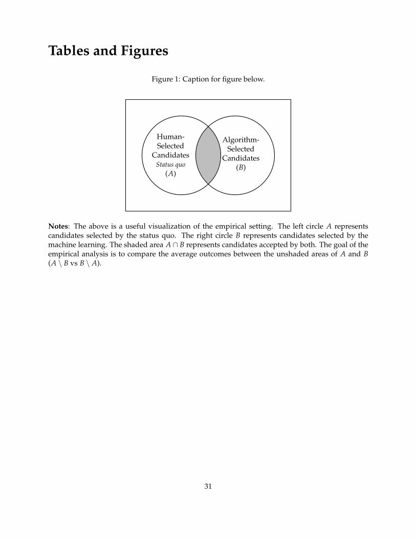
Tables and Figures

Figure 1: Caption for figure below.

Human-Selected

CandidatesStatus quo

(A)

Algorithm-Selected

Candidates(B)

Notes: The above is a useful visualization of the empirical setting. The left circle A representscandidates selected by the status quo. The right circle B represents candidates selected by themachine learning. The shaded area A ∩ B represents candidates accepted by both. The goal of theempirical analysis is to compare the average outcomes between the unshaded areas of A and B(A \ B vs B \ A).

31

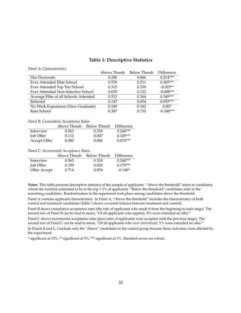
Table 1: Descriptive Statistics

Panel A: CharacteristicsAbove Thresh Below Thresh Difference

Has Doctorate 0.280 0.066 0.214***Ever Attended Elite School 0.576 0.211 0.365***Ever Attended Top Tier School 0.315 0.339 -0.025**Ever Attended Non-Selective School 0.035 0.122 -0.088***Average Elite of all Schools Attended 0.513 0.164 0.349***Referred 0.147 0.054 0.093***No Work Experience (New Graduate) 0.189 0.182 0.007Rare School 0.387 0.735 -0.348***

Panel B: Cumulative Acceptance RatesAbove Thresh Below Thresh Difference

Interview 0.563 0.318 0.244***Job Offer 0.112 0.007 0.105***Accept Offer 0.080 0.006 0.074***

Panel C: Incremental Acceptance RatesAbove Thresh Below Thresh Difference

Interview 0.563 0.318 0.244***Job Offer 0.199 0.020 0.179***Offer Accept 0.714 0.854 -0.140*

Notes: This table presents descriptive statistics of the sample of applicants. “Above the threshold” refers to candidateswhom the machine estimated to be in the top 1-2% of applicants. “Below the threshold” candidates refer to theremaining candidates. Randomization in the experiment took place among candidates above the threshold.

Panel A contains applicant characteristics. In Panel A, “Above the threshold” includes the characteristics of bothcontrol and treatment candidates (Table 2 shows covariate balance between treatment and control).

Panel B shows cumulative acceptance rates (the rate of applicants who made it from the beginning to each stage). Thesecond row of Panel B can be read to mean, “Of all applicants who applied, X% were extended an offer.”

Panel C shows incremental acceptance rates (pass rates of applicants were accepted until the previous stage). Thesecond row of Panel C can be read to mean, “Of all applicants who were interviewed, Y% were extended an offer.”

In Panels B and C, I include only the “Above” candidates in the control group because these outcomes were affected bythe experiment.

* significant at 10%; ** significant at 5%; *** significant at 1%. Standard errors are robust.

32

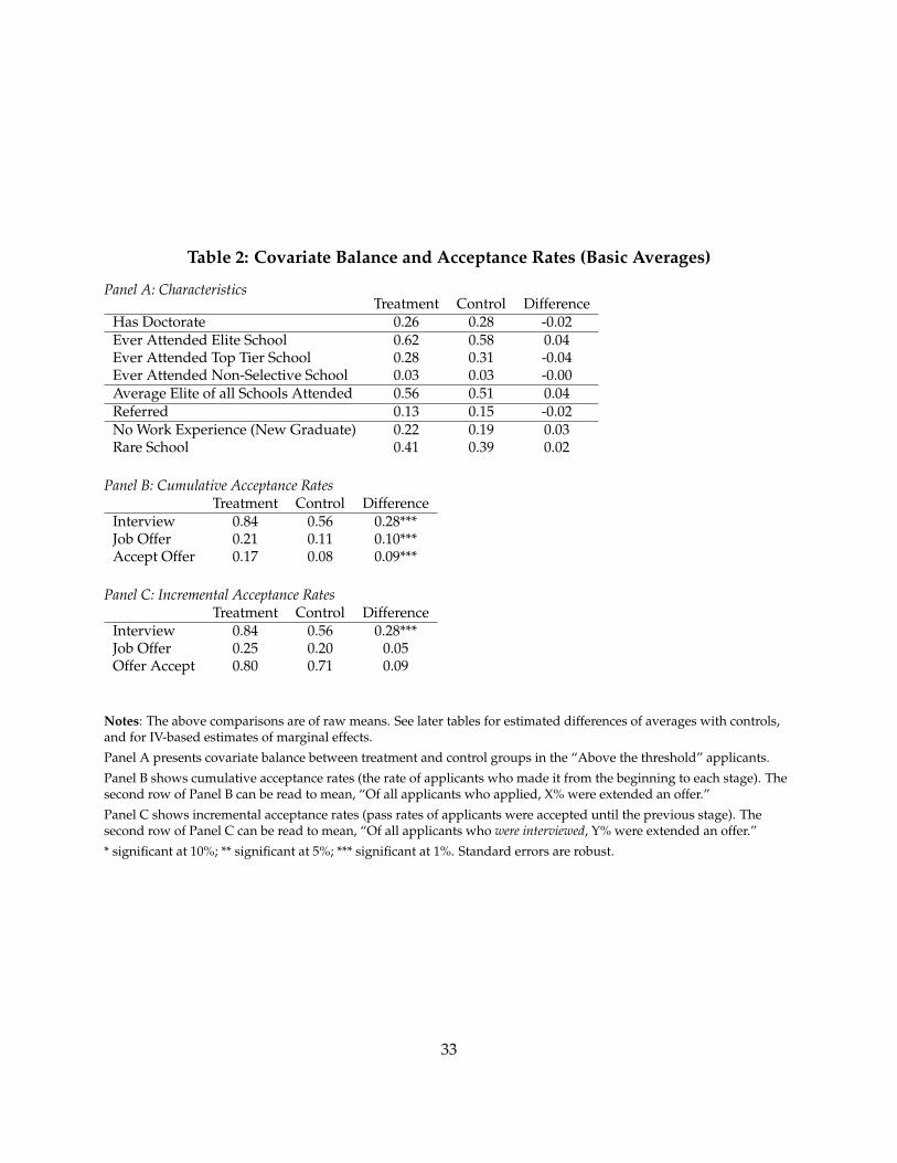
Table 2: Covariate Balance and Acceptance Rates (Basic Averages)

Panel A: CharacteristicsTreatment Control Difference

Has Doctorate 0.26 0.28 -0.02Ever Attended Elite School 0.62 0.58 0.04Ever Attended Top Tier School 0.28 0.31 -0.04Ever Attended Non-Selective School 0.03 0.03 -0.00Average Elite of all Schools Attended 0.56 0.51 0.04Referred 0.13 0.15 -0.02No Work Experience (New Graduate) 0.22 0.19 0.03Rare School 0.41 0.39 0.02

Panel B: Cumulative Acceptance RatesTreatment Control Difference

Interview 0.84 0.56 0.28***Job Offer 0.21 0.11 0.10***Accept Offer 0.17 0.08 0.09***

Panel C: Incremental Acceptance RatesTreatment Control Difference

Interview 0.84 0.56 0.28***Job Offer 0.25 0.20 0.05Offer Accept 0.80 0.71 0.09

Notes: The above comparisons are of raw means. See later tables for estimated differences of averages with controls,and for IV-based estimates of marginal effects.

Panel A presents covariate balance between treatment and control groups in the “Above the threshold” applicants.

Panel B shows cumulative acceptance rates (the rate of applicants who made it from the beginning to each stage). Thesecond row of Panel B can be read to mean, “Of all applicants who applied, X% were extended an offer.”

Panel C shows incremental acceptance rates (pass rates of applicants were accepted until the previous stage). Thesecond row of Panel C can be read to mean, “Of all applicants who were interviewed, Y% were extended an offer.”

* significant at 10%; ** significant at 5%; *** significant at 1%. Standard errors are robust.

33

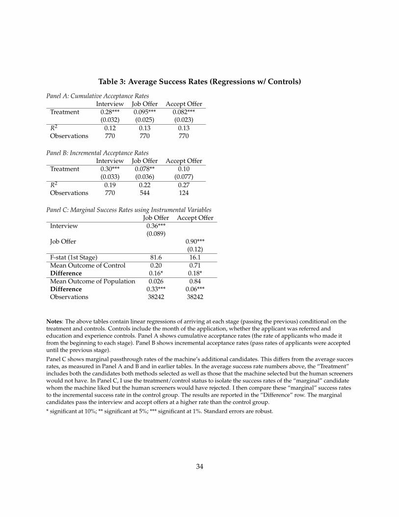
Table 3: Average Success Rates (Regressions w/ Controls)

Panel A: Cumulative Acceptance RatesInterview Job Offer Accept Offer

Treatment 0.28*** 0.095*** 0.082***(0.032) (0.025) (0.023)

R2 0.12 0.13 0.13Observations 770 770 770

Panel B: Incremental Acceptance RatesInterview Job Offer Accept Offer

Treatment 0.30*** 0.078** 0.10(0.033) (0.036) (0.077)

R2 0.19 0.22 0.27Observations 770 544 124

Panel C: Marginal Success Rates using Instrumental VariablesJob Offer Accept Offer

Interview 0.36***(0.089)

Job Offer 0.90***(0.12)

F-stat (1st Stage) 81.6 16.1Mean Outcome of Control 0.20 0.71Difference 0.16* 0.18*Mean Outcome of Population 0.026 0.84Difference 0.33*** 0.06***Observations 38242 38242

Notes: The above tables contain linear regressions of arriving at each stage (passing the previous) conditional on thetreatment and controls. Controls include the month of the application, whether the applicant was referred andeducation and experience controls. Panel A shows cumulative acceptance rates (the rate of applicants who made itfrom the beginning to each stage). Panel B shows incremental acceptance rates (pass rates of applicants were accepteduntil the previous stage).

Panel C shows marginal passthrough rates of the machine’s additional candidates. This differs from the average succesrates, as measured in Panel A and B and in earlier tables. In the average success rate numbers above, the “Treatment”includes both the candidates both methods selected as well as those that the machine selected but the human screenerswould not have. In Panel C, I use the treatment/control status to isolate the success rates of the “marginal” candidatewhom the machine liked but the human screeners would have rejected. I then compare these “marginal” success ratesto the incremental success rate in the control group. The results are reported in the “Difference” row. The marginalcandidates pass the interview and accept offers at a higher rate than the control group.

* significant at 10%; ** significant at 5%; *** significant at 1%. Standard errors are robust.

34

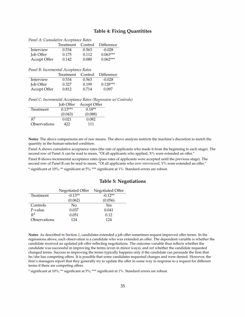
Table 4: Fixing Quantitites

Panel A: Cumulative Acceptance RatesTreatment Control Difference

Interview 0.534 0.563 -0.028Job Offer 0.175 0.112 0.063***Accept Offer 0.142 0.080 0.062***

Panel B: Incremental Acceptance RatesTreatment Control Difference

Interview 0.534 0.563 -0.028Job Offer 0.327 0.199 0.128***Accept Offer 0.812 0.714 0.097

Panel C: Incremental Acceptance Rates (Regression w/ Controls)Job Offer Accept Offer

Treatment 0.13*** 0.18**(0.043) (0.088)

R2 0.021 0.082Observations 422 111

Notes: The above comparisons are of raw means. The above analysis restricts the machine’s discretion to match thequantity in the human-selected condition.

Panel A shows cumulative acceptance rates (the rate of applicants who made it from the beginning to each stage). Thesecond row of Panel A can be read to mean, “Of all applicants who applied, X% were extended an offer.”

Panel B shows incremental acceptance rates (pass rates of applicants were accepted until the previous stage). Thesecond row of Panel B can be read to mean, “Of all applicants who were interviewed, Y% were extended an offer.”

* significant at 10%; ** significant at 5%; *** significant at 1%. Standard errors are robust.

Table 5: Negotiations

Negotiated Offer Negotiated OfferTreatment -0.13** -0.12**

(0.062) (0.056)Controls No YesP-value 0.037 0.041R2 0.051 0.12Observations 124 124

Notes: As described in Section 2, candidates extended a job offer sometimes request improved offer terms. In theregressions above, each observation is a candidate who was extended an offer. The dependent variable is whether thecandidate received an updated job offer reflecting negotiations. The outcome variable thus reflects whether thecandidate was successful in improving the terms (even in minor ways), and not whether the candidate requestedchanged terms. Success in improving the terms typically happens only if the candidate can persuade the firm thathe/she has competing offers. It is possible that some candidates requested changes and were denied. However, thefirm’s managers report that they generally try to update the offer in some way in response to a request for differentterms if there are competing offers.

* significant at 10%; ** significant at 5%; *** significant at 1%. Standard errors are robust.

35

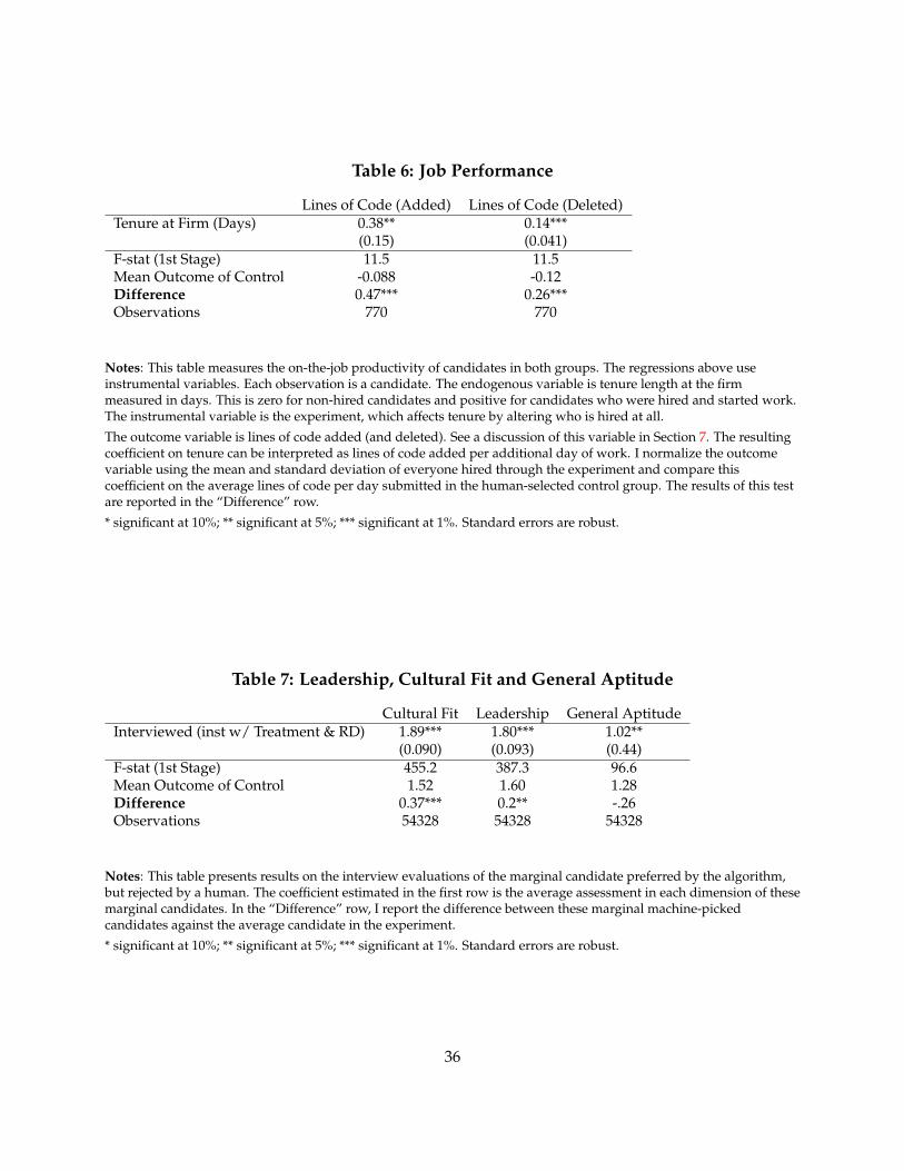
Table 6: Job Performance

Lines of Code (Added) Lines of Code (Deleted)Tenure at Firm (Days) 0.38** 0.14***

(0.15) (0.041)F-stat (1st Stage) 11.5 11.5Mean Outcome of Control -0.088 -0.12Difference 0.47*** 0.26***Observations 770 770

Notes: This table measures the on-the-job productivity of candidates in both groups. The regressions above useinstrumental variables. Each observation is a candidate. The endogenous variable is tenure length at the firmmeasured in days. This is zero for non-hired candidates and positive for candidates who were hired and started work.The instrumental variable is the experiment, which affects tenure by altering who is hired at all.

The outcome variable is lines of code added (and deleted). See a discussion of this variable in Section 7. The resultingcoefficient on tenure can be interpreted as lines of code added per additional day of work. I normalize the outcomevariable using the mean and standard deviation of everyone hired through the experiment and compare thiscoefficient on the average lines of code per day submitted in the human-selected control group. The results of this testare reported in the “Difference” row.

* significant at 10%; ** significant at 5%; *** significant at 1%. Standard errors are robust.

Table 7: Leadership, Cultural Fit and General Aptitude

Cultural Fit Leadership General AptitudeInterviewed (inst w/ Treatment & RD) 1.89*** 1.80*** 1.02**

(0.090) (0.093) (0.44)F-stat (1st Stage) 455.2 387.3 96.6Mean Outcome of Control 1.52 1.60 1.28Difference 0.37*** 0.2** -.26Observations 54328 54328 54328

Notes: This table presents results on the interview evaluations of the marginal candidate preferred by the algorithm,but rejected by a human. The coefficient estimated in the first row is the average assessment in each dimension of thesemarginal candidates. In the “Difference” row, I report the difference between these marginal machine-pickedcandidates against the average candidate in the experiment.

* significant at 10%; ** significant at 5%; *** significant at 1%. Standard errors are robust.

36

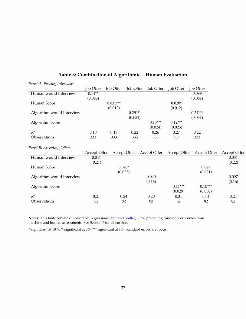
Table 8: Combination of Algorithmic + Human Evaluation

Panel A: Passing InterviewsJob Offer Job Offer Job Offer Job Offer Job Offer Job Offer

Human would Interview 0.14** 0.099(0.063) (0.061)

Human Score 0.031*** 0.020*(0.012) (0.012)

Algorithm would Interview 0.25*** 0.24***(0.051) (0.051)

Algorithm Score 0.13*** 0.12***(0.024) (0.025)

R2 0.18 0.18 0.22 0.26 0.27 0.22Observations 333 333 333 333 333 333

Panel B: Accepting OffersAccept Offer Accept Offer Accept Offer Accept Offer Accept Offer Accept Offer

Human would Interview 0.041 0.031(0.21) (0.22)

Human Score 0.040* 0.027(0.023) (0.021)

Algorithm would Interview 0.040 0.097(0.16) (0.16)

Algorithm Score 0.11*** 0.10***(0.029) (0.030)

R2 0.21 0.24 0.20 0.31 0.34 0.21Observations 82 82 82 82 82 82

Notes: This table contains “horserace” regressions (Fair and Shiller, 1989) predicting candidate outcomes frommachine and human assessments. See Section 7 for discussion.

* significant at 10%; ** significant at 5%; *** significant at 1%. Standard errors are robust.

37

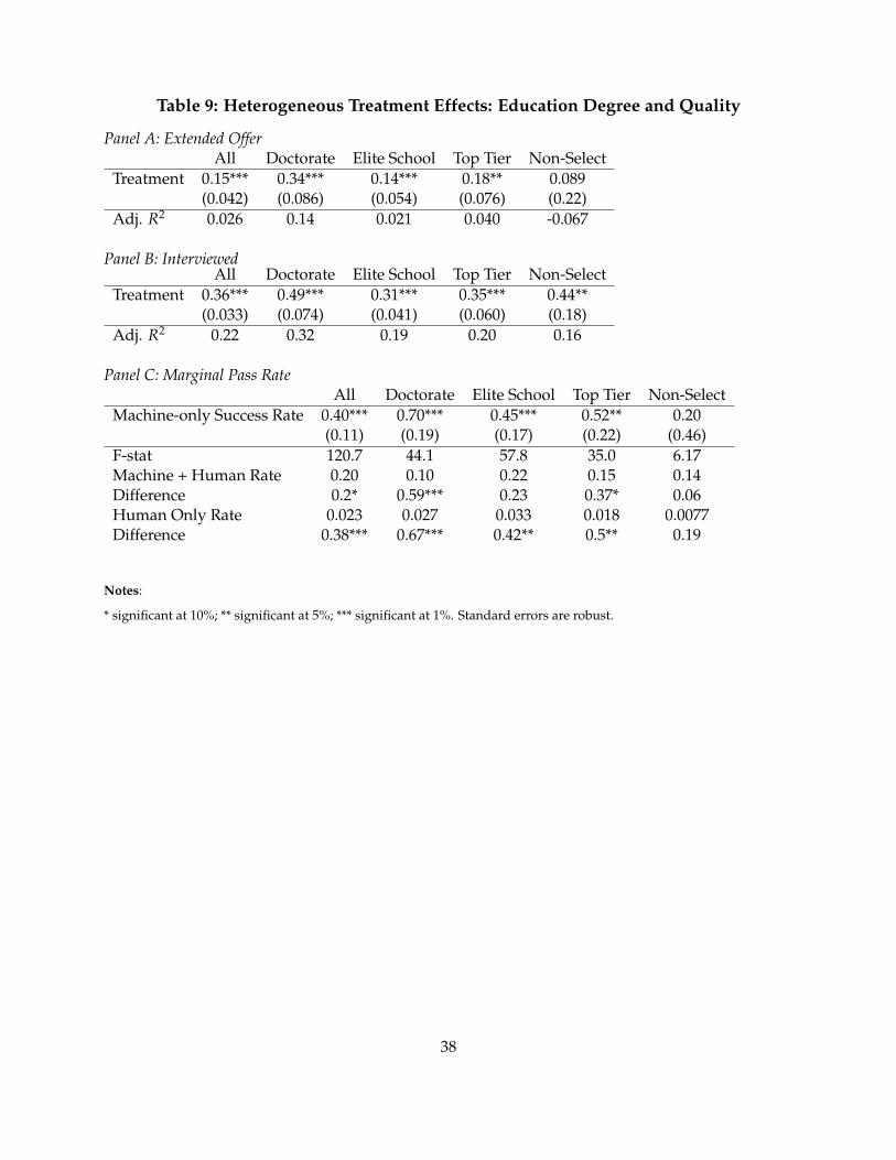
Table 9: Heterogeneous Treatment Effects: Education Degree and Quality

Panel A: Extended OfferAll Doctorate Elite School Top Tier Non-Select

Treatment 0.15*** 0.34*** 0.14*** 0.18** 0.089(0.042) (0.086) (0.054) (0.076) (0.22)

Adj. R2 0.026 0.14 0.021 0.040 -0.067

Panel B: InterviewedAll Doctorate Elite School Top Tier Non-Select

Treatment 0.36*** 0.49*** 0.31*** 0.35*** 0.44**(0.033) (0.074) (0.041) (0.060) (0.18)

Adj. R2 0.22 0.32 0.19 0.20 0.16

Panel C: Marginal Pass RateAll Doctorate Elite School Top Tier Non-Select

Machine-only Success Rate 0.40*** 0.70*** 0.45*** 0.52** 0.20(0.11) (0.19) (0.17) (0.22) (0.46)

F-stat 120.7 44.1 57.8 35.0 6.17Machine + Human Rate 0.20 0.10 0.22 0.15 0.14Difference 0.2* 0.59*** 0.23 0.37* 0.06Human Only Rate 0.023 0.027 0.033 0.018 0.0077Difference 0.38*** 0.67*** 0.42** 0.5** 0.19

Notes:

* significant at 10%; ** significant at 5%; *** significant at 1%. Standard errors are robust.

38

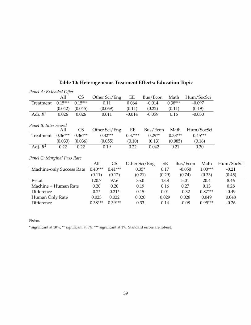
Table 10: Heterogeneous Treatment Effects: Education Topic

Panel A: Extended OfferAll CS Other Sci/Eng EE Bus/Econ Math Hum/SocSci

Treatment 0.15*** 0.15*** 0.11 0.064 -0.014 0.38*** -0.097(0.042) (0.045) (0.069) (0.11) (0.22) (0.11) (0.19)

Adj. R2 0.026 0.026 0.011 -0.014 -0.059 0.16 -0.030

Panel B: InterviewedAll CS Other Sci/Eng EE Bus/Econ Math Hum/SocSci

Treatment 0.36*** 0.36*** 0.32*** 0.37*** 0.29** 0.38*** 0.45***(0.033) (0.036) (0.055) (0.10) (0.13) (0.085) (0.16)

Adj. R2 0.22 0.22 0.19 0.22 0.042 0.21 0.30

Panel C: Marginal Pass RateAll CS Other Sci/Eng EE Bus/Econ Math Hum/SocSci

Machine-only Success Rate 0.40*** 0.41*** 0.35* 0.17 -0.050 1.00*** -0.21(0.11) (0.12) (0.21) (0.29) (0.74) (0.33) (0.45)

F-stat 120.7 97.6 35.0 13.8 5.01 20.4 8.46Machine + Human Rate 0.20 0.20 0.19 0.16 0.27 0.13 0.28Difference 0.2* 0.21* 0.15 0.01 -0.32 0.87*** -0.49Human Only Rate 0.023 0.022 0.020 0.029 0.028 0.049 0.048Difference 0.38*** 0.39*** 0.33 0.14 -0.08 0.95*** -0.26

Notes:

* significant at 10%; ** significant at 5%; *** significant at 1%. Standard errors are robust.

39

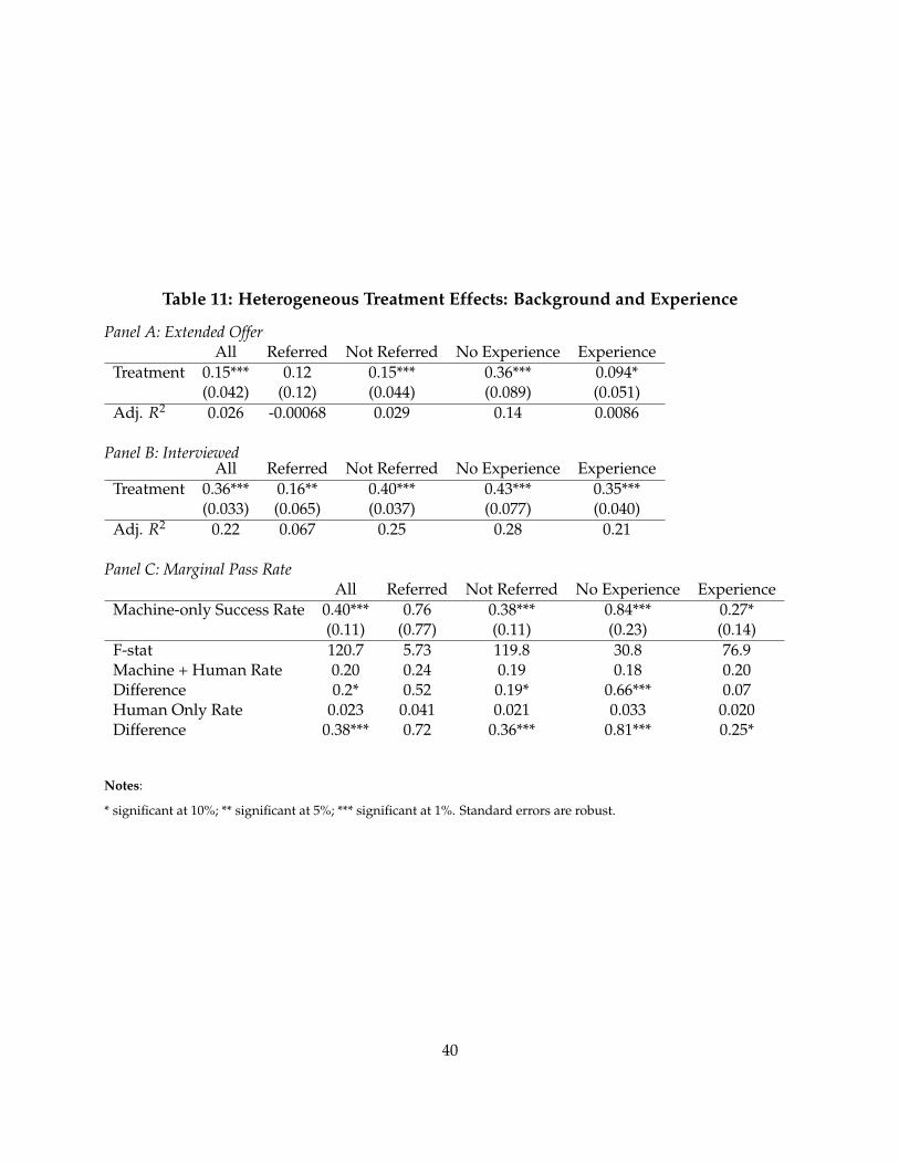
Table 11: Heterogeneous Treatment Effects: Background and Experience

Panel A: Extended OfferAll Referred Not Referred No Experience Experience

Treatment 0.15*** 0.12 0.15*** 0.36*** 0.094*(0.042) (0.12) (0.044) (0.089) (0.051)

Adj. R2 0.026 -0.00068 0.029 0.14 0.0086

Panel B: InterviewedAll Referred Not Referred No Experience Experience

Treatment 0.36*** 0.16** 0.40*** 0.43*** 0.35***(0.033) (0.065) (0.037) (0.077) (0.040)

Adj. R2 0.22 0.067 0.25 0.28 0.21

Panel C: Marginal Pass RateAll Referred Not Referred No Experience Experience

Machine-only Success Rate 0.40*** 0.76 0.38*** 0.84*** 0.27*(0.11) (0.77) (0.11) (0.23) (0.14)

F-stat 120.7 5.73 119.8 30.8 76.9Machine + Human Rate 0.20 0.24 0.19 0.18 0.20Difference 0.2* 0.52 0.19* 0.66*** 0.07Human Only Rate 0.023 0.041 0.021 0.033 0.020Difference 0.38*** 0.72 0.36*** 0.81*** 0.25*

Notes:

* significant at 10%; ** significant at 5%; *** significant at 1%. Standard errors are robust.

40

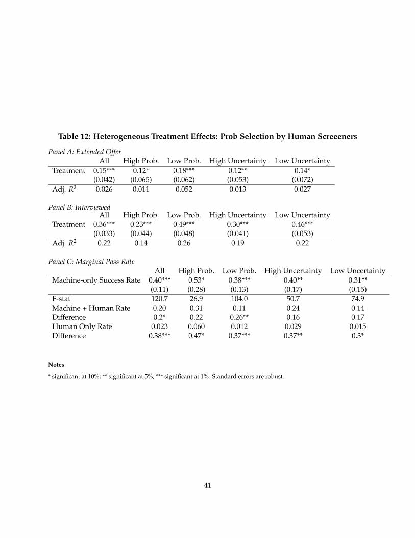
Table 12: Heterogeneous Treatment Effects: Prob Selection by Human Screeeners

Panel A: Extended OfferAll High Prob. Low Prob. High Uncertainty Low Uncertainty

Treatment 0.15*** 0.12* 0.18*** 0.12** 0.14*(0.042) (0.065) (0.062) (0.053) (0.072)

Adj. R2 0.026 0.011 0.052 0.013 0.027

Panel B: InterviewedAll High Prob. Low Prob. High Uncertainty Low Uncertainty

Treatment 0.36*** 0.23*** 0.49*** 0.30*** 0.46***(0.033) (0.044) (0.048) (0.041) (0.053)

Adj. R2 0.22 0.14 0.26 0.19 0.22

Panel C: Marginal Pass RateAll High Prob. Low Prob. High Uncertainty Low Uncertainty

Machine-only Success Rate 0.40*** 0.53* 0.38*** 0.40** 0.31**(0.11) (0.28) (0.13) (0.17) (0.15)

F-stat 120.7 26.9 104.0 50.7 74.9Machine + Human Rate 0.20 0.31 0.11 0.24 0.14Difference 0.2* 0.22 0.26** 0.16 0.17Human Only Rate 0.023 0.060 0.012 0.029 0.015Difference 0.38*** 0.47* 0.37*** 0.37** 0.3*

Notes:

* significant at 10%; ** significant at 5%; *** significant at 1%. Standard errors are robust.

41

Appendix

A Comparison to Dawes

42