available at iet digital library. physical emission of...
TRANSCRIPT

This paper is a postprint of a paper submitted to and accepted for publication in IET Radar, Sonar & Navigation and is subject to Institution of Engineering and Technology Copyright. The copy of record is
available at IET Digital Library.
This work was supported in part by the Air Force Office of Scientific Research, the Naval Research
Laboratory – Radar Division, and the Office of Naval Research base funding program. All views and
opinions expressed here are the authors’ own and do not reflect the official position of the U.S.
Department of Defense.
Portions of this paper were presented at the 2014 IEEE Radar Conference [1].
Physical Emission of Spatially-Modulated Radar
SHANNON D. BLUNT1
University of Kansas
PATRICK MCCORMICK2
University of Kansas
THOMAS HIGGINS3
US Naval Research Laboratory
MURALIDHAR RANGASWAMY4
US Air Force Research Laboratory
Leveraging the recent development of a physical implementation of arbitrary polyphase codes as
spectrally well-contained waveforms, the notion of spatial modulation is developed whereby a time-
varying beampattern is incorporated into the physical emission of an individual pulse. This subset of the
broad category of MIMO radar is inspired by the operation of fixational eye movement within the human
eye to enhance visual acuity and also subsumes the notion of the frequency-diverse array for application
to pulsed radar. From this spatial modulation framework some specific emission examples are evaluated
in terms of resolution and sidelobe levels for the delay and angle domains. The impact of spatial
modulation upon spectral content is also considered and possible joint delay-angle emission design
criteria are suggested. Simulation results of selected target arrangements demonstrate the promise of
enhanced discrimination and the basis for the development of future cognitive radar capabilities that may
mimic salient aspects of the visual cortex.
1Electrical Engineering & Computer Science Dept., 2335 Irving Hill Road, Lawrence, KS, 66045,
2Electrical Engineering & Computer Science Dept., 2335 Irving Hill Road, Lawrence, KS, 66045,
3Radar Division, Building 60, 4555 Overlook Ave. SW, Washington, DC, 20375,
4Sensors Directorate, Building 620, 2241 Avionics Circle, Wright-Patterson AFB, OH, 45433,

I. INTRODUCTION
Traditionally, electronically scanned radar systems emit a waveform-modulated pulse in a single
spatial direction by applying a fixed inter-element phase shift across the antenna array, with an otherwise
identical waveform being generated by each of the antenna elements. The received echoes are thus
likewise characterized by the same waveform response regardless of spatial direction. In contrast, the
notion of transmitting different, albeit correlated, waveforms from the elements of an array has been
proposed [2-12] as a method to broaden the transmit beamwidth (i.e. beam-spoiling) for the purpose of
achieving, for example, simultaneous multi-mode radar [12-15].
Here we consider the specific case in which the pulsed radar emission possesses both a temporal
modulation (the waveform) and an intra-pulse spatial modulation that can be viewed as a form of fast-time
time-division beamforming [5-12], a prominent example of which is the frequency-diverse array concept
[5-10]. The proposed spatial modulation scheme actually subsumes this frequency-diverse array concept
within the framework of pulsed emissions.
There is an interesting biological analog to this proposed scheme found in the visual system of humans
and other animals possessing fovea in which the particular direction of attention is spatially modulated in a
seemingly random manner (Fig. 1) via slow movements known as drift and rapid movements known as
microsaccades [1,16,17]. While the purpose of these fixational eye movements has long been debated and
remains an open research topic, the current consensus is that these small, spatial perturbations improve
visual acuity because the associated transients enhance contrast and sensitivity as well as aiding in the
resolving of spatial ambiguities. Furthermore, there is evidence [18] that these eye movements adapt
according to environmental conditions (e.g. amount of lighting) and the active attention of the observer
thereby suggesting a linkage between the physical actuation of the (passive) sensor and higher-level
cognition, which for the extension here to active sensing implies an application within the context of
cognitive radar [19].
With this visual/neurological antecedent as a source of inspiration, we consider the concept of fast-
time spatial modulation of a pulsed emission by employing an inter-element phase shift across the array

that varies over the duration of the pulsewidth. This emission strategy forms a subset of the more general
class of multiple-input multiple-output (MIMO) radar transmit schemes. Here, an approach denoted as the
waveform diverse array (WDA) is used to allow for selection and physical generation of an arbitrary FM-
based waveform while also providing control over the fast-time-dependent spatial beampattern during the
pulse. The characteristics of the WDA approach are assessed relative to the traditional beamformed
emission by examining the time-varying beampattern, aggregate beampattern, and an ambiguity function
that is dependent on delay, transmit spatial angle, and receive spatial angle. A framework for determining
the impact of spatial modulation on spectral content is also developed.
Figure 1 Example of small eye movements during fixation
The diversity afforded by this spatially-modulated emission strategy is achieved by coupling the spatial
angle and delay (range) domains and is conceptually similar to the angle-Doppler coupling of clutter that
occurs for ground moving target indication (GMTI) from an airborne/space-based platform, for which the
development of space-time adaptive processing (STAP) was necessitated. It is demonstrated that the
interaction between the waveform and spatial modulation structures can produce joint emissions in which
both delay and angle sidelobe reduction is achieved and spatial resolution is enhanced with only the use of
angle-dependent receiver matched filtering (i.e. without adaptive receive processing).

The remainder of the paper is organized as follows. Section II introduces the WDA scheme for
physical generation of spatially-modulated emissions, along with associated performance metrics, analysis
of spectral content, and evaluation of some exemplary cases. In Section III simulation results are presented
for different scattering scenarios with the various emission schemes to assess the impact of spatial
modulation in the delay and angle domains and the diversity enhancement it affords for sensing. Section
IV summarizes the observations of spatial modulation and discusses areas of ongoing/future work.
II. WAVEFORM DIVERSE ARRAY (WDA)
The biological counterpart of fixational eye movement clearly suggests the use of a two-dimensional
array (for spatial modulation in azimuth and elevation). While the WDA concept is applicable to any array
geometry, for the sake of illustration we shall herein focus on the uniform linear array (ULA). The array
element spacing is denoted as d with spatial angle defined relative to array boresight (at which 0 ).
It is assumed that emitted/received signals satisfy the array narrowband assumption and thus the associated
electrical phase angle is 2 sin( ) /d , with the wavelength of the carrier frequency.
A. WDA Definition
The waveform diverse array (WDA) concept employs an independent waveform generator behind each
element of the antenna array. To link the phase modulation of the waveform with the element-wise spatial
modulation in fast-time we leverage the continuous phase modulation (CPM) framework described in
[20,21] that generates polyphase-coded FM (PCFM) waveforms (Fig. 2). First, given a polyphase radar
code with the 1N phase values 0 1, , , N , a train of N impulses with time separation pT are
formed such that the total pulsewidth is pT NT . The thn impulse is weighted by n , which is the
phase change between successive polyphase code values as determined by
if
2 sgn if
n nn
n n n
, (1)
where

1n n n for 1, ,n N , (2)
and sgn( ) is the signum operation. The shaping filter ( )g t may, for example, be rectangular or raised
cosine with the requirements 1) that it integrates to unity over the real line; and 2) that it has time support
on [0, ]pT . The PCFM waveform is thus
w 0
10
( ; ) exp ( ) ( 1)
t N
n p
n
s t j g n T d
x , (3)
where denotes convolution, 0 is the initial phase value of the code, and the sequence of phase changes
are collected into the vector w 1 2
T
N x which parameterizes the complex baseband
waveform.
Figure 2 CPM implementation to generate polyphase-coded FM (PCFM) waveforms
This framework can likewise be extended to parameterize in a physical manner the fast-time
modulation of relative phase across the antenna array to facilitate spatial modulation during the pulse.
Here a spatial modulation code comprised of 1N values 0 1, , , N is defined as a sequence of
spatial angle offsets relative to some center direction C . The subsequent spatial phase-change sequence
(as a function of code index n) for use with the CPM implementation and a uniform linear array is thus
C C 1
2sin( ) sin( )n n n
d
for 1, ,n N , (4)
noting that the values n can be positive or negative and are small enough (when combined with C ) to
avoid spatial “wrap around” beyond the endfire directions at 90 . Echoing the structure of (3), the
spatial phase modulation as a function of continuous time is therefore

s 0
10
( ; ) exp ( ) ( 1)
t N
n p
n
b t j g n T d
x (5)
where the sequence of spatial phase changes are collected into the vector s 1 2
T
N x and the
initial electrical angle is
0 C 0
2sin
d
. (6)
The leading negative sign within the exponential of (5), relative to the waveform representation in (3),
reflects the phase delay compensation for spatial beamsteering on transmit.
For the M antenna elements, define the half-wavelength-based position indexing as
0.5( 1), 0.5( 1) 1, , 0.5( 1) m M M M so that 0m is located at the center of the array,
the indices are both positive and negative, and the indices increment by one. Note that when M is an
even number, these indices will be offset by 1/2. This imposed symmetry is useful for physical intuition of
the emission structure and is convenient for analysis of the impact on bandwidth for spatial modulation
(Section II.C).
The signal generated by the antenna element with thm position index is thus
C w s w s
1( , ; , ) ( ; ) ( ; ) x x x x
mms t s t b t
T, (7)
where the normalization term provides unit transmit energy per antenna element and the Vandermonde-like
form ( )m across the uniform linear array yields, from (7),
s 0
10
( ; ) exp ( ) ( 1)
t Nm
n p
n
b t jm g n T d
x . (8)
In the case of no spatial modulation, we have 0 1 0N so that, from (4),
1 2 0N likewise and (6) becomes 0 C2 sin /d . As a result, (8) simplifies to
s 0( ; ) expmb t jm x , which is simply the phase delay on the thm indexed antenna element needed
to steer a stationary beam in the direction of spatial angle C (i.e. standard beamforming).
Finally, if we insert (3) and (8) into (7) the continuous CPM-implemented signal generated by the thm
indexed antenna element can be expressed as

C w s 0 0
10
1( , ; , ) exp ( ) ( 1)
x x
t N
m n n p
n
s t j g m n T d mT
. (9)
In other words, defining for the thm indexed antenna element a joint phase-change sequence
, n m n nm and initial phase 0, 0 0 m m , the CPM radar implementation from Fig. 2 can
be used with these values at each antenna element to produce the associated physical emission without
needing an additional modulation stage in hardware.
It should also be noted that, as demonstrated by widespread use of CPM for applications such as
aeronautical telemetry [22], deep space communications [23], and BluetoothTM
wireless [24], the radar-
centric implementation in Fig. 2 is essentially a manifestation of FM that does not require the use of an
arbitrary waveform generator (AWG), thereby avoiding the potentially high cost of deploying numerous
AWGs for a MIMO radar to produce many different waveforms simultaneously. Furthermore, the
emission scheme of (9) avoids the large phase differences between adjacent antenna elements that could
otherwise cause radiation outside of real space which may damage the radar [25].
B. WDA Beampattern and Ambiguity Analysis
The WDA emission can be assessed by examining the time-varying beampattern, aggregate
beampattern, and the angle-delay ambiguity function. These metrics are based on the normalized baseband
representation of the composite far-field emission for time t and spatial angle defined as
( 1)/2
2 sin( )/C
( 1)/2
1, , ( , )
M
jm dC m
m M
g t s t eM
, (10)
where C( , )ms t is taken from (9) and the exponential term is the delay resulting from path length
differences as a function of angle . Note that the dependence on the waveform code wx and spatial
modulation code sx have been suppressed for the sake of compact representation. If the set of M
waveforms C( , )ms t are identical aside from a scalar phase shift (no spatial modulation applied) then the
emission , , Cg t is just the original waveform ( )s t beamformed in the direction C , i.e. the temporal
modulation is decoupled from the spatial angle. Otherwise, however, a different temporal waveform will
be observed at different spatial angles in the far-field.

Using (10), the instantaneous spatial features generated with the WDA can be examined using the
time-varying beampattern (TVBP) denoted as
, , , , , , TV C C CB t g t g t (11)
for 0 t T , where *
denotes complex conjugation. Integrating (11) over the pulse width and
dividing by T yields the aggregate beampattern
0
1, , , , ,
T
C C CB g t g t dtT
. (12)
As discussed above, if no spatial modulation is present the product , , , ,
C Cg t g t is a constant
over the pulse width such that , CB yields the usual array factor beampattern [26] steered to C .
On receive (and assuming negligible Doppler shift of the resulting echoes during the pulsewidth), the
reflected signal incident upon the thm indexed antenna element can be expressed as
2 sin( )/C C, ( , ) ( , , ) ( )
jm dmy t x t g t e d u t , (13)
where ( , )x t is the complex scattering as a function of time (delay) and spatial angle, ( )u t is additive
noise, and represents convolution. Receive beamforming (in direction ) and pulse compression can
be performed as
( 1)/2
2 sin( )/
( 1)/2
1, , ( , )
M
jm dC m C
m M
z t y t eM
(14)
and
*ˆ( , , ) , , ( , , )C C Cx z t h t dt , (15)
respectively, where ( , , )Ch t is the pulse compression filter for receive angle and is the relative
delay of the incident signal. The true matched filter for (15) would be ( , , ) ( , , )C Ch t g t .
However, because of the angle-delay coupling induced by spatial modulation it is useful to normalize the
matched filter such that the gain is constant as a function of receive angle to avoid artificially scaling the
estimated scattering response and the noise. As such, we define a unity-gain normalized matched filter as

1/2
0
, ,, ,
, , , ,
CC
T
C C
g th t
g t g t dt
(16)
so that (15) actually provides the matched filter estimate of the illumination-scaled response
1/2
0
( , , ) ( , , ) , , , ,
T
C C C Cx x g t g t dt
. (17)
Using the coherent receive processing defined in (14)-(16), an angle-delay ambiguity function (ADAF)
can be constructed as
2( 1)/2
*
( 1)/20
1/2
*C C
0
, , , ,
,
, , ,
,
,
,
T Mjm jm
C C
m M
CT
g t e g t e dt
A
M g t g t dt
(18)
where the electrical angle corresponding to a signal arriving from spatial angle is
2
sind
, (19)
and the electrical angle corresponding to the receive filter tuned to spatial angle is
2
sind
. (20)
Note that due to the normalization factors in (7), (10), (14), and (16), the case of standard beamforming (no
spatial modulation) realizes a response for (18) at 0 and that achieves the maximum value of
unity. Thus the “beam smearing” loss of spatial modulation can be directly determined. Also, while not
considered here, Doppler can be readily incorporated into (18) to obtain an angle-delay-Doppler ambiguity
function. Finally, as long as the array narrowband assumption holds, this emission and subsequent analysis
framework can be easily modified for arbitrary array structures.
C. WDA Spectral Impact
The spatial modulation in (7) also produces a convolution in frequency that serves to expand the
bandwidth relative to standard beamforming (using the same waveform). The emissions from the outer
elements of the array, having the largest indices of ( 1) / 2m M in (8), thus exhibit the largest
additional spectral excursion from the carrier frequency. Here we examine the degree of bandwidth
expansion for the illustrative example of a linear frequency modulated (LFM) waveform and linearly
scanning spatial modulation, where the latter subsumes the frequency diverse array framework [5-12] for a
pulsed emission. This example then permits the statement of a general bandwidth expansion expression.
Relative to the center direction C , with associated electrical angle C via (19), consider the spatial
deviation over the interval corresponding to the first nulls in either direction. Define null,+ and null, as
the positive and negative spatial angle deviations corresponding to the first nulls that respectively realize
the electrical angles
null,+ null,+
null, null,
2sin( )
2sin( )
C
C
d
d . (21)
For M antenna elements with inter-element separation d the electrical angle phase change that results
from traversing from one first-null to the other is proportional to 2 /Md [26] as
null,+ null, null,+ null,
2 2 2sin( ) sin( )
4
C C
d d
Md
M
. (22)
Generalizing (22) to the traversal of K null-to-null intervals thus realizes an electrical angle phase change
of 4 /K M , where 0 / 2K M (and K need not be an integer) with the upper limit corresponding to a
boresight center direction with spatial traversal from one endfire direction to the other during the pulse.
From an “energy on target” perspective and in light of the small perturbations observed for fixational eye
movement [16-18], it seems likely that one would wish K to be relatively small (perhaps 1 ).

Using (4) and (8), the outermost elements scale the electrical angle phase change by the largest value
of ( 1) / 2M so that, based on (22), the total electrical angle phase change at these elements when
traversing K null-to-null spatial intervals is
4 1outer elements phase change 2
2
MK K
M
(23)
for M sufficiently large. For the case of linear spatial modulation over the pulsewidth and under the
assumption that K and C are such that a linear spatial angle traversal corresponds sufficiently well to a
linear electrical angle phase change, then at the outer antenna elements the spatial modulation induces a
frequency shift upon the underlying waveform w( ; )xs t in the amount of
2 2 /outer element frequency shift
p
K K N
T T, (24)
where we have used the relationship pT NT defined for the CPM implementation. The numerator in
(24) corresponds to the nm term in (9) when ( 1) / 2m M so that
2 1 4
2 1
n
K M K
N N M. (25)
As demonstrated in (25) for linear spatial modulation, n is a constant as a function of time index n. It
is important to note, however, that for a linear frequency modulated (LFM) waveform implemented with
CPM, the values of n exhibit a uniform sampling on the interval , as a function of n [27,28].
Furthermore, as defined by the structure of the CPM implementation in (1)-(3), the maximum phase
changes over the transition interval pT are for the LFM waveform. These limits on the phase change
were defined in [21] to aid in spectral containment but there is no physical or mathematical reason why
they cannot be exceeded (see [29] for further discussion of this “over-coding” effect).
Combining the waveform and spatial modulations as ( ) n nm from (9) and using the maximum
phase transitions for each via (25), ( 1) / 2m M , and n , we find that the maximum total
instantaneous phase changes over the transition interval pT , which otherwise establish the outermost
frequency components of the emission (therefore demarcating the bandwidth), are thus

(2 / )outermost frequencies
p
K N
T. (26)
In other words, relative to traditional beamforming, linear spatial modulation of an LFM waveform
involves a bandwidth increase by a factor of
2 (2 / )(linear) bandwidth increase factor 1 2 /
2
K NK N , (27)
where the leading 2 in the numerator and denominator arises from the attribute of (26) and the phase-
change support of ,n for LFM implemented using CPM.
In general for an arbitrary waveform and spatial modulation implemented using (9), the total
bandwidth increase can be expressed as
(general) bandwidth increase factor
max ( 1)/2 min ( 1)/2
max min
n n n n
n n
M M (28)
where n need not be a constant (i.e. can be nonlinear spatial modulation). The bandwidth metric in (28)
also implies that joint optimization of the waveform and spatial modulations via selection of n and n
for 1, ,n N may be performed in such a way as to bound the total bandwidth by establishing a
constraint relationship between each of the [ , ] n n pairs.
D. WDA Emission Evaluation
To demonstrate the attributes of this spatially-modulated emission scheme, we employ the CPM
implementation (via (3)) of a length N = 200 code wx to produce a LFM waveform (CPM very closely
approximates LFM akin to a first-order hold representation using linear phase segments that can be made
arbitrarily small). The antenna array is a M = 30 element uniform linear array with half-wavelength
element spacing and with C 0 (i.e. boresight center direction). Thus null-to-null spatial scanning
( 1K ) comprises 3.8 in spatial angle. The pulsewidth is set to 1T for convenience of illustration.
Using this known waveform we consider four cases of spatial modulation. In Case 1 standard
stationary beamforming is used to provide a baseline for comparison. In contrast, Case 2 employs spatial

modulation over the pulsewidth and scans linearly from 1st null to 1
st null (on each side). Likewise, Case 3
uses linear spatial scanning, albeit from 2nd
null to 2nd
null relative to C 0 (so 2K ). Finally, Case 4
considers spatial modulation involving a half cycle of a sinusoid that is likewise centered on C 0 and
with maximum spatial excursions of the 1st nulls occurring at the beginning and end of the pulse.
Figure 3 illustrates the time-varying beampattern from (11) for each of the four cases. As one would
expect from an instantaneous perspective, the spatial mainbeam and sidelobes retain the same structure
across the four cases, albeit tilted or twisted according to the spatial modulation structure. When the
beampattern is considered in aggregate over the pulsewidth, the spatial modulation has the effect of
“smearing” the beam as shown in Fig. 4 resulting in an aggregate mainbeam that is lower and wider than
that of the standard beamforming case. Clearly a peak SNR penalty results at C from using spatial
modulation. However, in contrast to what the aggregate beampattern appears to indicate, spatial
modulation can in fact enhance spatial resolution due to angle-delay coupling.

Figure 3 Time-varying beampattern (TVBP) for Case 1) standard beamforming, Case 2) null-to-null linear
spatial modulation, Case 3) double null-to-null linear spatial modulation, and Case 4) null-to-null half-
cycle sinusoidal spatial modulation
Figure 4 Aggregate beampattern for Case 1) standard beamforming, Case 2) null-to-null linear spatial
modulation, Case 3) double null-to-null linear spatial modulation, and Case 4) null-to-null half-cycle
sinusoidal spatial modulation

To examine the impact of delay-angle coupling it is instructive to consider various cuts of the
ambiguity function in (18). Figure 5 depicts the delay matched point ( 0 ) for the four emission
schemes as a function of transmit angle and receive angle . Here it is observed that relative to
standard beamforming (Case 1) the spatial modulation Cases 2-4 exhibit a mainbeam that is elongated
along the axis while the sidelobes not on this axis are markedly lower. In other words, for transmit
angles that are different from a given receive angle , spatial modulation can result in a lower cross-
correlation of the associated angle-dependent waveforms.
Figure 5 0 cut of angle-delay ambiguity function for Case 1) standard beamforming, Case 2) null-to-
null linear spatial modulation, Case 3) double null-to-null linear spatial modulation, and Case 4) null-to-
null half-cycle sinusoidal spatial modulation
Taking the 0 cut of the responses in Fig. 5 and peak-normalizing for easy comparison yields the
results shown in Figs. 6 and 7. In Fig. 6 we find that, relative to the peak, the sidelobes of the three spatial
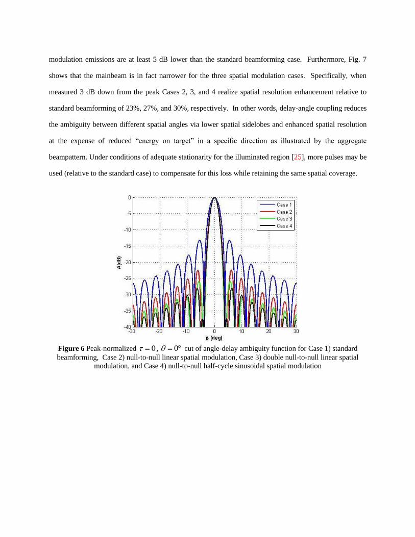
modulation emissions are at least 5 dB lower than the standard beamforming case. Furthermore, Fig. 7
shows that the mainbeam is in fact narrower for the three spatial modulation cases. Specifically, when
measured 3 dB down from the peak Cases 2, 3, and 4 realize spatial resolution enhancement relative to
standard beamforming of 23%, 27%, and 30%, respectively. In other words, delay-angle coupling reduces
the ambiguity between different spatial angles via lower spatial sidelobes and enhanced spatial resolution
at the expense of reduced “energy on target” in a specific direction as illustrated by the aggregate
beampattern. Under conditions of adequate stationarity for the illuminated region [25], more pulses may be
used (relative to the standard case) to compensate for this loss while retaining the same spatial coverage.
Figure 6 Peak-normalized 0 , 0 cut of angle-delay ambiguity function for Case 1) standard
beamforming, Case 2) null-to-null linear spatial modulation, Case 3) double null-to-null linear spatial
modulation, and Case 4) null-to-null half-cycle sinusoidal spatial modulation

Figure 7 Peak-normalized 0 , 0 cut of angle-delay ambiguity function (mainbeam close-up) for
Case 1) standard beamforming, Case 2) null-to-null linear spatial modulation, Case 3) double null-to-null
linear spatial modulation, and Case 4) null-to-null half-cycle sinusoidal spatial modulation
It is also instructive to consider the angle-delay ambiguity as a function of and for the 0
cut (Fig. 8) where it is interesting to note the lack of observable range sidelobes for the spatial modulation
cases (2-4). It is important to point out, however, that this result is specific to the particular waveform and
spatial modulations shown here and would differ for various waveform/spatial modulation combinations.
If we select the 0 cut of the response in Fig. 8 for closer inspection, the delay dimension can be
isolated as shown in Fig. 9. Of the four, standard beamforming (Case 1) clearly exhibits the best range
resolution. That said, the spatial modulation schemes examined here realize orders-of-magnitude lower
range sidelobes at the expense of some degradation in range resolution (and peak power as previously
indicated). These cases produce an effect akin to waveform amplitude tapering, albeit with this effect
being produced by spatial modulation in the far field as opposed to actual amplitude weighting in the
transmitter that would otherwise preclude the operation of power amplifiers in saturation.
Note that not all means of spatial modulation necessarily provide a range sidelobe improvement. It
was shown in [1] that a full-cycle sinusoid produced very high near-in range sidelobes. This effect could
be the result of re-traversing the same spatial angles in the second half of the sinusoidal cycle so that the
range-angle ambiguity is dominated by the cross-correlation of the associated waveform segments that

share the same spatial angles. Thus if spatial modulation is to be used, the joint waveform/spatial
modulation structure must be considered.
Figure 8 0 cut of angle-delay ambiguity function for Case 1) standard beamforming, Case 2) null-
to-null linear spatial modulation, Case 3) double null-to-null linear spatial modulation, and Case 4) null-to-
null half-cycle sinusoidal spatial modulation

Figure 9 0 , 0 cut of angle-delay ambiguity function for Case 1) standard beamforming, Case
2) null-to-null linear spatial modulation, Case 3) double null-to-null linear spatial modulation, and Case 4)
null-to-null half-cycle sinusoidal spatial modulation
Finally, Figs. 10-13 depict spectral content (normalized by pulsewidth T ) for the four cases. For Case
1 (Fig. 10) the same waveform is emitted by every antenna element so only the single spectral plot is
shown for baseline comparison. For Cases 2-4 the spectral content is depicted in Figs. 11-13 for the
emissions from the outermost elements of the length 30M uniform linear array along with a center-
most element emission for comparison, which by the enforced symmetry will experience negligible effects
from spatial modulation for the cases considered. For the ease of the reader, the elements are labeled from
left-to-right as 1, 2, ,30 with element 15 used as the center-most element. In terms of the position
indexing previously defined, the elements shown are indices 0.5(29) 14.5m (1st element),
0.5(29) 14 0.5m (15th element), and 0.5(29) 29 14.5m (30
th element).
The LFM waveform implemented here with CPM is constructed from a 200N code [21] thus
yielding a time-bandwidth product of 200BT as evidenced by the pulsewidth-normalized 3 dB

bandwidth for the standard beamforming case in Fig. 10. Defining an aggregated bandwidth as that
established by the 3 dB collective bandwidths demarcated by the outermost element emissions, it is found
in Fig. 11 that the normalized aggregated bandwidth for the null-to-null linear spatial modulation of Case 2
is 202, a 1% increase over standard beamforming which agrees with (27). Likewise, the (Case 3) double
null-to-null linear spatial modulation result in Fig. 12 realizes a normalized aggregated bandwidth of 204, a
2% increase as predicted by (27). For the half-cycle sinusoidal Case 4 we must use the more general (28).
However, this case experiences negligible spatial modulation at the beginning and ends of the pulse (per
examination of Fig. 3) where LFM yields the greatest excursions from the center frequency. Thus, as
observed in Fig. 13, the half-cycle sinusoidal spatial modulation combined with an LFM waveform
exhibits no bandwidth increase.
To demonstrate the utility of (28) consider the full-cycle sinusoid spatial modulation examined in [1]
where the extremum values of ( ) n nm are found to be 3.237 (in radians) thereby predicting a 3%
increase in aggregated bandwidth. This prediction agrees with the result in Fig. 14 that depicts a
normalized aggregated bandwidth of 206.
Figure 10 Normalized spectral content for Case 1) standard beamforming – normalized bandwidth = 200
(baseline case)

Figure 11 Normalized spectral content for Case 2) null-to-null linear spatial modulation – aggregated
normalized bandwidth = 202 (or 1% bandwidth increase)
Figure 12 Normalized spectral content for Case 3) double null-to-null linear spatial modulation –
aggregated normalized bandwidth = 204 (or 2% bandwidth increase)

Figure 13 Normalized spectral content for Case 4) null-to-null half-cycle sinusoidal spatial modulation –
aggregated normalized bandwidth = 200 (so no bandwidth increase)
Figure 14 Normalized spectral content for Case 4) null-to-null sinusoidal spatial modulation – aggregated
normalized bandwidth = 206 (or 3% bandwidth increase)
These cases were selected to provide a snapshot of the diverse possible emission structures that may be
achieved by combining spatial and waveform modulations. From a cognitive sensing perspective one can

envision the development of a set of underlying code pairs w s( , )x x that possess different degrees of range
and spatial resolution and sidelobe characteristics. In fact, considering a tracking modality in which some
prior knowledge may be presumed with regard to target number and range-angle dispositions within a local
region based on previous state estimates, code pairs could potentially be defined that enhance, in a
scenario-dependent manner, the range-angle discrimination of targets for enhanced tracking performance.
III. SIMULATION RESULTS
In Section II.D the spatial modulation structure was assessed with regard to the characteristics of
different joint delay-angle emission schemes. Here we consider these emission schemes in terms of the
output of receive processing for a couple representative target scenarios. In the first scenario two targets
are present at the same range with angular separation commensurate with the spatial resolution of standard
beamforming. In the second scenario five targets are present that form a ‘X’ in range and angle to illustrate
the impact of the different emission schemes in both dimensions. In both cases the targets possess a
receive SNR that is 20 dB following coherent integration (based on individual standard beamforming for
each target). The same emission parameterization as Section II.D is used so N = 200 (which approximates
the waveform time-bandwidth product) and the antenna is comprised of M = 30 elements with half-
wavelength spacing. For both scenarios the center direction is set to C 0 such that the first nulls are
3.8 in spatial angle.
Due to the pulsed nature of the radar, Nyquist receive sampling can only be approximated, though the
good spectral containment of the CPM implementation [21] certainly helps to keep the “over-sampling”
relative to the 3 dB bandwidth to a nominal level. For the results shown the receiver matched filtering is
performed for a sampling rate that is three times that of the 3 dB waveform bandwidth. As such, a
waveform generated from code length N = 200 realizes a matched filter with a discretized length of 600.

A. Two Targets at Same Range
Consider two targets occupying the same range (range index 200) and at spatial angles of 2
(roughly nominal resolution for 30M element array). The targets are in-phase which is known to be the
most difficult case for achieving separation using beamforming. Figure 15 shows the delay-angle response
from beamforming and pulse compression as defined in (14)-(16) for the four spatial modulation schemes
described in Fig. 3. For standard beamforming (Case 1) we only observe a single target centered in
between the two true angles because the target angles correspond to the nominal resolution separation and
are in-phase (thus inhibiting their separation). However, when the emission is the null-to-null linear spatial
modulation of Case 2, we find that the two targets are now clearly visible. The double null-to-null linear
modulated emission of Case 3 likewise realizes two separate targets, though SNR is noticeably reduced
relative to Case 2 due to greater energy dispersal across spatial angle (unnecessarily in this case). Finally,
Case 4 shows the response of the null-to-null half-cycle sinusoidal spatial modulation which appears to
provide marginally the best overall performance of these four considered based on the shape and
disposition of the matched filter response.

Figure 15 Two-target scenario for Case 1) standard beamforming, Case 2) null-to-null linear spatial
modulation, Case 3) double null-to-null linear spatial modulation, and Case 4) null-to-null half-cycle
sinusoidal spatial modulation
B. Five Targets in a Range-Angle “X” Arrangement
Now consider five targets phase in an ‘X’ pattern where two of the targets occupy the same range
(index 196) at spatial angles 3 , a center target resides at range index 200 at spatial angle 0 , and two
more targets occupy range index 204 at spatial angles 3 . Each target phase is randomly assigned yet
remains fixed for the four emission schemes considered to provide a fair comparison. Figure 16 reveals
the results for this scenario. For standard beamforming (Case 1) the center target at 0 spatial angle is
clearly shown, though the other four targets at different spatial angles are not visible aside from a smaller
response that may be from the top-left target in the ‘X’. In contrast, the null-to-null linear spatial
modulation (Case 2) does capture all five target echoes, though they are not necessarily distinguishable as
separate. The double null-to-null linear spatial modulation (Case 3), on the other hand, exhibits greater

smearing than the previous linear case and reveals no evident response from the lower-left target. Finally,
the half-cycle sinusoid spatial modulation (Case 4) appears to be quite similar to the linear emission of
Case 2, which upon comparison of their fast-time beam trajectories from Fig. 3 is not unexpected.
Figure 16 Five-target ‘X’ scenario for Case 1) standard beamforming, Case 2) null-to-null linear spatial
modulation, Case 3) double null-to-null linear spatial modulation, and Case 4) null-to-null half-cycle
sinusoidal spatial modulation
It should be noted that the random phase relationship between the targets does have an effect on how
well these closely-spaced targets can be identified, which is also dependent upon the spatial modulation
scheme; thus the single instantiation depicted in Fig. 16 is an incomplete characterization. To provide a
somewhat broader characterization and also to demonstrate how spatial modulation may exploit the phase
diversity of multiple targets, consider the response from four consecutive pulses of each emission scheme
upon the same five-target ‘X’ scenario under the condition that the target phases are likewise randomly

(and independently) assigned for each pulse. Note that this randomly varying phase condition is not meant
to represent a particular operational radar mode or scenario but is simply being used as a generic example.
Because no knowledge is presumed regarding the targets’ pulse-to-pulse phase responses, non-coherent
integration of the echoes from the four pulses is used to compare the four emission schemes.
Figure 17 illustrates the results of the four spatial modulation schemes after non-coherent integration
over four pulses. Standard beamforming (Case 1) now realizes a “halo effect” surrounding the center
target with an SNR of about 8 dB (compared to the 20 dB center target response). While this halo could be
viewed as potentially indicative of surrounding targets, it is far from conclusive evidence. In stark contrast
to standard beamforming the result for the linear spatial modulation of Case 2 now reveals all five targets,
albeit with a shallow null between the leftmost top and bottom targets. The target resolvability is less
prominent for the double linear (Case 3) and half-cycle sinusoid (Case 4) spatial modulations, yet all five
target responses are still evident. Clearly, this enhancement would not have occurred if the relative target
phases were coherent with one another from pulse to pulse, though that may be an extreme case depending
upon the radar modality. However, it is anticipated that using a different spatial modulation scheme on
each pulse followed by appropriate combining could provide even further benefit as a result of the
additional diversity of pulse agility (and it would not rely upon phase diversity of the targets).

Figure 17 Four-pulse non-coherent integration of five-target ‘X’ scenario for Case 1) standard
beamforming, Case 2) null-to-null linear spatial modulation, Case 3) double null-to-null linear spatial
modulation, and Case 4) null-to-null half-cycle sinusoidal spatial modulation
IV. CONCLUSIONS
Spatially modulating emissions during a pulse provides a form of MIMO radar that is consistent with the passive
sensing paradigm of fixational eye movement found in nature. The resulting waveform-diverse array (WDA)
concept presented here that is based on the continuous phase modulation (CPM) code-to-waveform implementation
subsumes the frequency-diverse array concept for pulsed radar operation and also facilitates a general framework in
which the joint delay-angle characteristics may be designed. A prospective application may be the incorporation of
cognition into radar tracking, particularly of multiple proximate targets, by leveraging the operation of the visual
cortex for an active sensing paradigm. It has been shown that different spatial modulation structures, when coupled
with a standard LFM waveform, allow for different trade-offs in terms of resolution and sidelobe levels in both the
delay and angle domains due to their inherent coupling. Further, the aggregate bandwidth over the collection of

emissions across the array is dependent on the relationship between the spatial and waveform modulations.
Considering that the one-dimensional spatial array defined here can be readily extended to a two-dimensional planar
array to enable spatial modulation in both azimuth and elevation and that the CPM implementation permits the
implementation of arbitrary polyphase codes as transmitter-amenable waveforms, this joint (now delay-azimuth-
elevation) emission structure establishes a very rich design space in which to explore new physically-realizable
MIMO emission schemes. Ongoing work is exploring how the diversity afforded by this delay-angle coupling can
be exploited to enhance target discrimination within a coherent processing interval of multiple pulses, how pulse
agility may be incorporated, and how the development of a set of such waveform/spatial modulation emission pairs
may be used for “on-the-fly” interrogation within a cognitive radar context.
References
[1] Blunt, S.D., McCormick, P., Higgins, T., Rangaswamy, M., “Spatially-modulated radar waveforms
inspired by fixational eye movement,” IEEE Radar Conference, Cincinnati, OH, 19-23 May 2014.
[2] Stoica, P. Li, J., Xie, Y. “On probing signal design for MIMO radar,” IEEE Trans. Signal Processing, vol.
55, pp. 4151-4161, Jan. 2008.
[3] Fuhrmann, D., Browning, J.P., Rangaswamy, M., “Constant-modulus partially correlated signal design for
uniform linear and rectangular MIMO radar arrays,” Intl. Waveform Diversity and Design Conf., Orlando,
FL, 9-13 Feb. 2009.
[4] Fuhrmann, D., San Antonio, G., “Transmit beamforming for MIMO radar systems using signal cross
correlations,” IEEE Trans. Aerospace & Electronic Systems, vol. 44, pp. 171-186, Jan. 2008.
[5] Antonik, P., Wicks, M.C., Griffiths, H.D., Baker, C.J., “Range-dependent beamforming using element
level waveform diversity,” Intl. Waveform Diversity and Design Conf., Lihue, HI, 22-27 Jan. 2006.
[6] Baizert, P., Hale, T.B., Temple, M.A., Wicks, M.C., “Forward-looking radar GMTI benefits using a linear
frequency diverse array,” IEE Electronics Letters, vol. 42, pp. 1311-1312, Oct. 2006.
[7] Secmen, M., Demir, S., Hizal, A., Eker, T., “Frequency diverse array antenna with periodic time modulated
pattern in range and angle,” IEEE Radar Conf., Waltham, MA, 17-20 Apr. 2007.
[8] Higgins, T., Blunt, S.D., “Analysis of range-angle coupled beamforming with frequency-diverse chirps,”
Intl. Waveform Diversity & Design Conf., Orlando, FL, pp. 140-144, 8-13 Feb. 2009.
[9] Sammartino, P.F., Baker, C.J., Griffiths, H.D., “Frequency diverse MIMO techniques for radar,” IEEE
Trans. Aerospace & Electronic Systems, vol. 49, no. 1, pp. 201-222, Jan. 2013.
[10] Wang, W.-Q., “Phased-MIMO radar with frequency diversity for range-dependent beamforming,” IEEE
Sensors Journal, vol. 13, no. 4, pp. 1320-1328, Apr. 2013.
[11] Duly, A.J., Love, D.J., Krogmeier, J.V., “Time-division beamforming for MIMO radar waveform design,”
IEEE Trans. Aerospace & Electronic Systems, vol. 49, no. 2, pp. 1210-1223, Apr. 2013.
[12] Antonik, P., Wicks, M.C., Griffiths, H.D., Baker, C. J., “Multi-mission multi-mode waveform diversity,”
IEEE Radar Conf., Verona, NY, 24-27 Apr. 2006.

[13] Goodman, N.A., Stiles, J.M., “Resolution and synthetic aperture characterization of sparse radar arrays,”
IEEE Trans. Aerospace & Electronic Systems, vol. 39, no. 3, pp. 921-935, July 2003.
[14] Stiles, J., Sinha, V., Nanda, A.P., “Space-time transmit signal construction for multi-mode radar,” IEEE
Radar Conf., Verona, NY, 24-27 Apr. 2006.
[15] Kapfer, R.M., Davis, M.E., “Ultra wideband, multi-mode radar processing,” IEEE Radar Conf., Atlanta,
GA, pp. 95-100, 7-11 May 2012.
[16] Rolfs, M., “Microsaccades: small steps on a long way,” Vision Research, vol. 49, pp. 2415-2441, 2009.
[17] Ahissar, E., Arieli, A., “Seeing via miniature eye movements: a dynamic hypothesis for vision,” Frontiers
in Computational Neuroscience, vol. 6, no. 89, Nov. 2012.
[18] Cui, J., Wilke, M., Logothetis, N.K., Leopold, D.A., Liang, H., “Visibility states modulate microsaccade
rate and direction,” Vision Research, vol. 49, pp. 228-236, 2009.
[19] Haykin, S., Xue, Y., Setoodeh, P., “Cognitive radar: step toward bridging the gap between neuroscience
and engineering,” Proc. IEEE, vol. 100, no. 11, pp. 3102-3130, Nov. 2012.
[20] Jakabosky, J., Anglin, P., Cook, M., Blunt, S.D., Stiles, J., “Non-linear FM waveform design using
marginal Fisher’s information within the CPM framework,” IEEE Radar Conf., Kansas City, MO, 23-27
May 2011.
[21] Blunt, S.D., Cook, M., Jakabosky, J., de Graaf, J., Perrins, E., “Polyphase-coded FM (PCFM) waveforms:
part I: implementation,” IEEE Trans. Aerospace & Electronic Systems, vol. 50, no. 3, pp. 2219-2230, July
2014.
[22] IRIG Standard 106-00: Telemetry Standards, Range Commanders Council Telemetry Group, Range
Commanders Council, White Sands Missile Range, New Mexico.
[23] Bandwidth-Efficient Modulations: Summary of Definitions, Implementation, and Performance, Report
Concerning Space Data System Standards, Informational Report CCSDS 413.0-G-2.
[24] Specifications of the Bluetooth System, Bluetooth Special Interest Group, ver. 1.2, Nov. 2003.
[25] Daum, F., Huang, J., “MIMO radar: snake oil or good idea?” IEEE Aerospace and Electronic Systems
Magazine, vol. 24, no. 5, pp. 8-12, May 2009.
[26] Van Trees, H.L., Optimum Array Processing, John Wiley & Sons, 2002, Chap. 2.
[27] Jakabosky, J., Blunt, S.D., Cook, M.R., Stiles, J., Seguin, S.A., “Transmitter-in-the-loop optimization of
physical radar emissions,” IEEE Radar Conf., Atlanta, GA, 7-11 May 2012.
[28] Blunt, S.D., Cook, M., Jakabosky, J., de Graaf, J., Perrins, E., “Polyphase-coded FM (PCFM) waveforms:
part II: optimization,” IEEE Trans. Aerospace & Electronic Systems, vol. 50, no. 3. pp. 2231-2242, July
2014.
[29] Jakabosky, J., Blunt, S.D., Himed, B., “Optimization of “over-coded” radar waveforms,” IEEE Radar
Conference, Cincinnati, OH, 19-23 May 2014.