avoiding numerical pitfalls in social force models
TRANSCRIPT
PHYSICAL REVIEW E 87, 063305 (2013)
Avoiding numerical pitfalls in social force models
Gerta Koster,* Franz Treml, and Marion GodelDepartment of Computer Science and Mathematics, Munich University of Applied Sciences, 80335 Munich, Germany
(Received 16 January 2013; published 14 June 2013)
The social force model of Helbing and Molnar is one of the best known approaches to simulate pedestrianmotion, a collective phenomenon with nonlinear dynamics. It is based on the idea that the Newtonian laws ofmotion mostly carry over to pedestrian motion so that human trajectories can be computed by solving a setof ordinary differential equations for velocity and acceleration. The beauty and simplicity of this ansatz arestrong reasons for its wide spread. However, the numerical implementation is not without pitfalls. Oscillations,collisions, and instabilities occur even for very small step sizes. Classic solution ideas from molecular dynamicsdo not apply to the problem because the system is not Hamiltonian despite its source of inspiration. Looking atthe model through the eyes of a mathematician, however, we realize that the right hand side of the differentialequation is nondifferentiable and even discontinuous at critical locations. This produces undesirable behaviorin the exact solution and, at best, severe loss of accuracy in efficient numerical schemes even in short rangesimulations. We suggest a very simple mollified version of the social force model that conserves the desireddynamic properties of the original many-body system but elegantly and cost efficiently resolves several of theissues concerning stability and numerical resolution.
DOI: 10.1103/PhysRevE.87.063305 PACS number(s): 02.60.−x, 89.40.−a, 95.75.Pq, 45.70.Vn
I. INTRODUCTION
There are many approaches to modeling pedestrian dynam-ics [1–4]. Among them social force models are well established[5,6]. Their proximity to equations derived from Newton’slaws of motion allow direct application of standard numericalmethods, such as Euler’s method, to solve the equations thatare available through toolboxes such as Matlab, Mathematica,or numerical libraries. Nonetheless, scientists and tool userscontinue to run into trouble when implementing or employingthe model [7,8].
While the physical properties of the model that do notmatch human behavior, such as inertia, have been discussedto some extent [8], very little attention has yet been paid tothe mathematical properties and the resulting effects on thestability of the supposed exact solution and numerical solutionattempts. In fact, the authors are not aware of a general proofof existence for the solution. Discussions of stability refer tostrongly simplified one-dimensional problems [9].
The social force model resembles a Newtonian systemwithout being Hamiltonian itself. Energy conservation isdestroyed by friction and an upper limit for pedestrian speed.See [10,11] for extensive discussions of Hamiltonian systems.Hence, classic methods from molecular dynamics that makeuse of the Hamiltonian form do not target the problem and weneed to look for other solution options.
In this work, we point out several mathematical propertiesof the right hand side of the social force model’s set ofdifferential equations that lead to oscillations in the solutionand loss of accuracy in the numerical approximation. Asa matter of fact, the discrete difference equations that thenumerical schemes correspond to have solutions that do notonly quantitatively differ from the supposed solution of thesocial force model, but also qualitatively. This backgroundanalysis is described in Sec. II. In Sec. III, we suggestways to mollify the right hand side so that the difficulties
disappear, while the desired properties of the original modelare conserved. In Sec. IV, we demonstrate the success ofour ideas by comparing numerical solutions of both modelsat strategically important locations in very simple simulationscenarios that allow isolating the underlying problems.
Finally, in Sec. V, we compare results for the classic andthe mollified model in a typical bottleneck scenario takenfrom [12]. We use numerical schemes with step sizes thatproduce errors of comparable size as long as no singularity isencountered. Not only do the results for the mollified modelprove to be more natural but, in addition, we are able to utilizea much more efficient fifth order Runge-Kutta scheme savingconsiderable simulation time.
II. PROBLEM ANALYSIS
A. Original social force model of Helbing and Molnar
This work is built upon the original equations as theywere presented in [5] and in Molnar’s dissertation [13]. Weare aware that most simulation tools based on the social forcemodel (SFM) use variations of the base model. But, thesevariations still have the essential properties of the original andhence will experience similar difficulties.
We look at vectors x,v ∈ R2×m that denote the location andvelocity of pedestrians 1, . . . ,m in two-dimensional Euclideanspace. Vertical movement is neglected. To make sure thatthe speed of an individual j does not exceed an acceptableupper limit vmax,j , we need the auxiliary velocity w in themathematical formulation. Note that imposing a limit onpedestrian speed introduces a first deviation from Newtonianmechanics. When the speed is cut off without compensation,energy is lost. Following [5], we set vmax,j = 1.3 v0,j wherev0,j is each pedestrian’s individual free-flow velocity. Hence,pedestrians can accelerate but will not sprint. For the j thpedestrian, we have
xj = vj (wj ) :={
wj if ‖wj‖ < vmax,j
v0,j
‖wj ‖wj otherwise.(1)
063305-11539-3755/2013/87(6)/063305(13) ©2013 American Physical Society
GERTA KOSTER, FRANZ TREML, AND MARION GODEL PHYSICAL REVIEW E 87, 063305 (2013)
The following set of equations for x and w forms the actualsocial force model:
x = v(w),(2)
w = F (x,w) = Ftarget(x,w) + Fped(x,w) + Fob(x,w).
Ftarget, Fped, and Fob stand for forces acting on each pedestrianfrom the attracting target(s), repelling fellow pedestrians, andrepelling obstacles. Forces are assumed to obey a superpositionprinciple. Since there are usually several interacting pedestri-ans and several obstacles, Fped and Fob are sums of force termsFped,i,j and Fob,k . Fped and Fob are expressed as the gradients(in x) of suitable potentials, but not Ftarget as we will discussin Sec. II B.
Most of our observations are best presented when thesystem is reduced to the bare essentials. Hence, we willassume one target, one or two pedestrians depending on thescenario, and no obstacle, all unless otherwise stated. Theresulting mathematical claims can easily be carried over tomore complex situations.
B. Behavior at the target: Discontinuity of the right hand side
In this section, we will look at the seemingly trivial situationof one pedestrian moving towards one target in a space free ofobstacles. We may drop the index for the pedestrian and forcetypes. We also neglect, for the moment, that the velocity isbounded but will come back to the implications of the cutofffunction in Sec. II D. We consider the simplified equations
(x1,x2) = (v1,v2),(3)
(v1,v2) = F ((x1,x2),(v1,v2)).
Without loss of generality, we set the target location to (0,0).Force F then has the form
F (x,v) = 1
τ
(− x
‖x‖v0 − v
). (4)
The free-flow velocity v0 is the presumed walking velocity ofan individual across an open space. In practical applications,the free-flow velocities are usually assumed to be normallydistributed about a measured mean [14]. Negative free-flowvelocities and free-flow velocities above the sprint worldrecord should be excluded. The influence of the reaction timeτ modeled by prefactor 1
τis not relevant for our investigations
at the moment and τ is set to 0.5 (seconds) as suggestedin [5] throughout the paper. Again, in practical simulations,the reaction time should be individually set.
Stating a problem in dimensionless form often makes iteasier to focus. In the case of a single pedestrian with just onetarget, this can be achieved by the transformations t = 1
τt for
a dimensionless speed, x = xτv0
for a dimensionless pedestrianposition leading to v = v
v0as dimensionless speed. For the
equations we return to x and v as variables. The dimensionlesssystem is
x = v, v =(
− x
‖x‖ − v
). (5)
The simplified model versions in Eqs. (3) and (5) highlightthat, while inspiration for the social force model stems frommolecular dynamics, it is not, in itself, a Hamiltonian system.That is, there is no Hamiltonian function H (x,v) to rewrite thesystem in the form
x = ∇vH (x,v), v = −∇xH (x,v) (6)
and to represent energy. From (6) follows that the Hamiltonianmust have the form
H (x,v) = 12 〈v,v〉 + G(x) (7)
for some G. See [10] for a longer discussion. With this, theterm − 1
τv in (4) can not be produced. In fact, term − 1
τv
introduces “friction” and destroys energy conservation; sodoes the speed cutoff in Eq. (1). This means that the wealthof methods developed to conserve physical quantities thatare characteristic for the Hamiltonian systems of moleculardynamics do not target the social force model. In fact, theyvery often explicitly use the separable form of the Hamiltonfunction (7). Prominent examples are symplectic splittingmethods that conserve the volume in phase space. They aredescribed in [10] or [11].
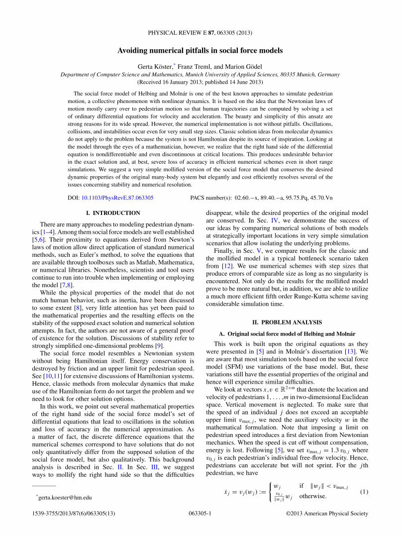
So, instead of trying to reproduce physical conservationlaws that do not apply for pedestrian motion, we turn ourattention to a straightforward analysis of the mathematicalproperties of the system: unit vectors −x/‖x‖ point in thedirection of the the target for all locations x �= (0,0). However,the function F has a singularity at the target x = (0,0). Theright hand side displays a jump (see Fig. 1).
1.0 0.5 0.0 0.5 1.0
1.0
0.5
0.0
0.5
1.0
1.0 0.5 0.0 0.5 1.01.5
1.0
0.5
0.0
0.5
1.0
1.5
x1
dire
ctio
nalv
ecto
rx
xfo
rx 2
0
FIG. 1. (Color online) Discontinuity in the right hand side of the social force model at the target. Left: vector plot. Right: cut with theplane x2 = 0.
063305-2
AVOIDING NUMERICAL PITFALLS IN SOCIAL FORCE . . . PHYSICAL REVIEW E 87, 063305 (2013)
Singularities in an equation do not necessarily shockthe practical user nor do they keep a model from beinguseful. However, they do have consequences, some of themundesirable. In our case, the disadvantages are twofold:
Loss of smoothness. A jump in the derivative means thatthe solution, if it exists, is at best continuous, certainly notdifferentiable. Such a solution can only exist in a weak sense.
Loss of accuracy and speed of convergence. More importantto the practical user is the loss of accuracy, in fact ofconvergence, of numerical schemes near discontinuities. Thismeans that, whenever a virtual person in the social forcemodel comes close to an intermediate target, or any otherpoint with insufficient smoothness in F , the trajectories andthe velocities will no longer be well resolved even with verysmall step sizes �t . Oscillations and even collisions in thenumerical approximation of the supposed true trajectories arethe result. This happens even at a very short range. It alsomeans that higher order, fast converging schemes, such as theRunge-Kutta methods, can not unfold their potential and one isstuck with slow converging schemes such as Euler’s method.We demonstrate this in Sec. IV. In the worst case, numericalerror or, more likely, the force of another pedestrian may causea virtual person to stumble right on the target point, or veryclose to it. This would lead to numerical division by zero. Ina practical simulation, one observes wild oscillations in thepedestrian trajectories or even that one virtual pedestrian is“blown away” from the target. In fact, it is not difficult toconstruct a “pathological” example using the Euler schemefor the numerical solution as we see in Sec. II B1.
One may argue that a virtual person can be removed fromthe simulation in time before he or she reaches the target.This means that the set of differential equations must bereinitialized with one less person. In fact, after reinitialization,we have a new and slightly different set of equations witha different solution. This constitutes a drawback, but maywork from a practical perspective as long as one does notuse intermediate targets to guide the virtual pedestrians alonga desired path and around obstacles. However, intermediatetargets are almost indispensable in practical applications. Anearly handover to the next target as soon as it is within sight,which is equivalent to another reinitialization and switch to aslightly altered initial value problem, helps. It is also naturalfrom a modeling point of view: Pedestrians like to navigatealong a graph where the points of orientation are connectedby a direct line of sight [15]. However, this is still trickyto handle. A lot of manual calibration for each intermediatetarget may become necessary to get just the right handovermoment: On the one hand, one strives to avoid the numericallydifficult close vicinity of the target. On the other hand, therisk of losing sight of the new intermediate target increaseswith early handover. Another person might “push” the virtualpedestrian out of the direct line of sight and he or she becomestrapped. Thus, once several pedestrians are competing forspace at the intermediate target exerting forces on each other,the calibration may become dysfunctional. We show a situationwhere this happens in Sec. V.
1. Explicit Euler scheme: Stable orbits around the target
The solution of the difference equations that stems fromdiscretizing a differential equation through a numerical scheme
need not conserve the behavioral properties of the originalequation. This happens to be the case when one applies Euler’sexplicit method on (3). Applying a k-step numerical schemeon a differential equation
y = F(y) (8)
means to discretize the equation in time. In the case of Euler’smethod, the result simply is
yn = yn−1 + �tF(yn−1), (9)
where yn is the solution one step ahead in time from yn−1 and�t is the step size in time.
Even with a consistent numerical scheme, such as Euler’smethod, there is no guarantee that the solution of the differenceequation has the same properties as the (supposed) solutionof the differential equation, unless a number of restrictingconditions on the smoothness of the right hand side aresatisfied. In the case of the social force model with itsdiscontinuity in the right hand side at the target point, andnondifferentiability at several other locations, we do not profitfrom such a comfortable situation.
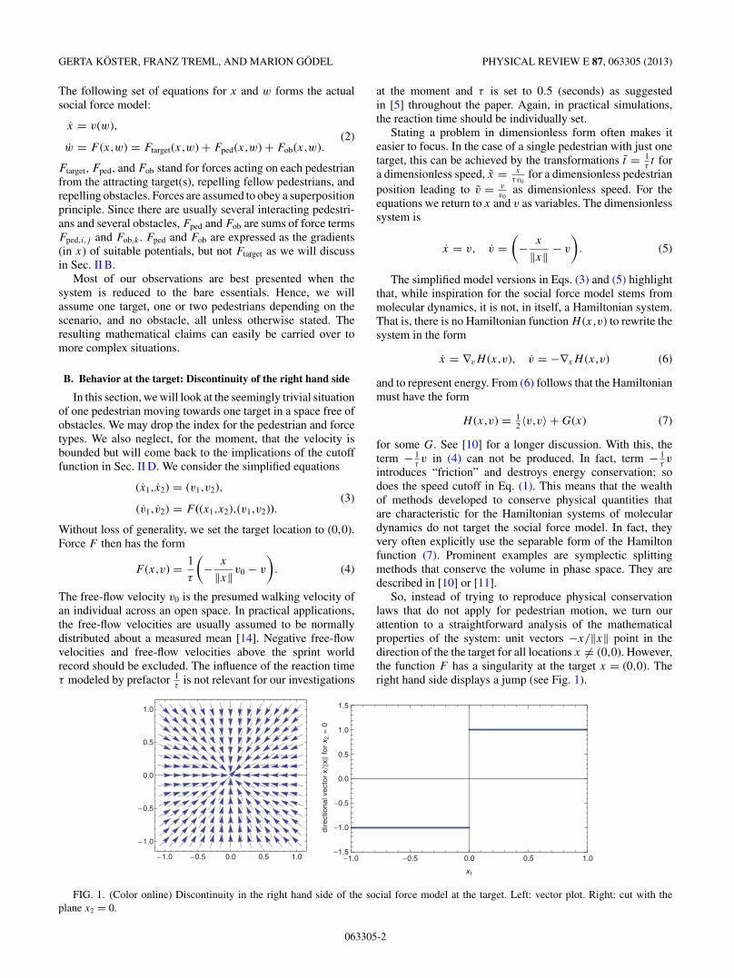
Indeed, the explicit Euler scheme which is widely popularin the social force community, despite its poor speed of con-vergence, reveals very undesirable behavior. The trajectoriesof the corresponding difference equation show a stable orbitaround the target. They do not, as required, approach thetarget when time goes to infinity. A particularly bad caseis easily constructed with with τ = 0.5, free-flow velocityv0 = 1, step size �t = 0.5, and initial values x = (0.25,0) andv = (1,0). The Euler scheme produces alternating values withx1 ∈ {−0.75,−0.25,0.25,0.75}, v1 ∈ {−1,1} and x2 = 0 andv2 = 0 for all iterations. Since the pedestrians keep movingat full speed, that is 1 m/s, each step in time corresponds toa stride with fixed length 0.5 m. Obviously, the pedestrianswill never get close to the target. Even worse, with (x,v) =[(0.5,0),(−1,0)] as starting point, the second iteration landsexactly on the target x = (0,0) leading to division by zero andabortion of the simulation run. The step sizes in these bad caseexamples are admittedly coarse but serve to demonstrate theprinciple, namely, that the numerical solution may never getclose to the target but may oscillate around it at considerablespeed or, even worse, that division by zero is quite possible.
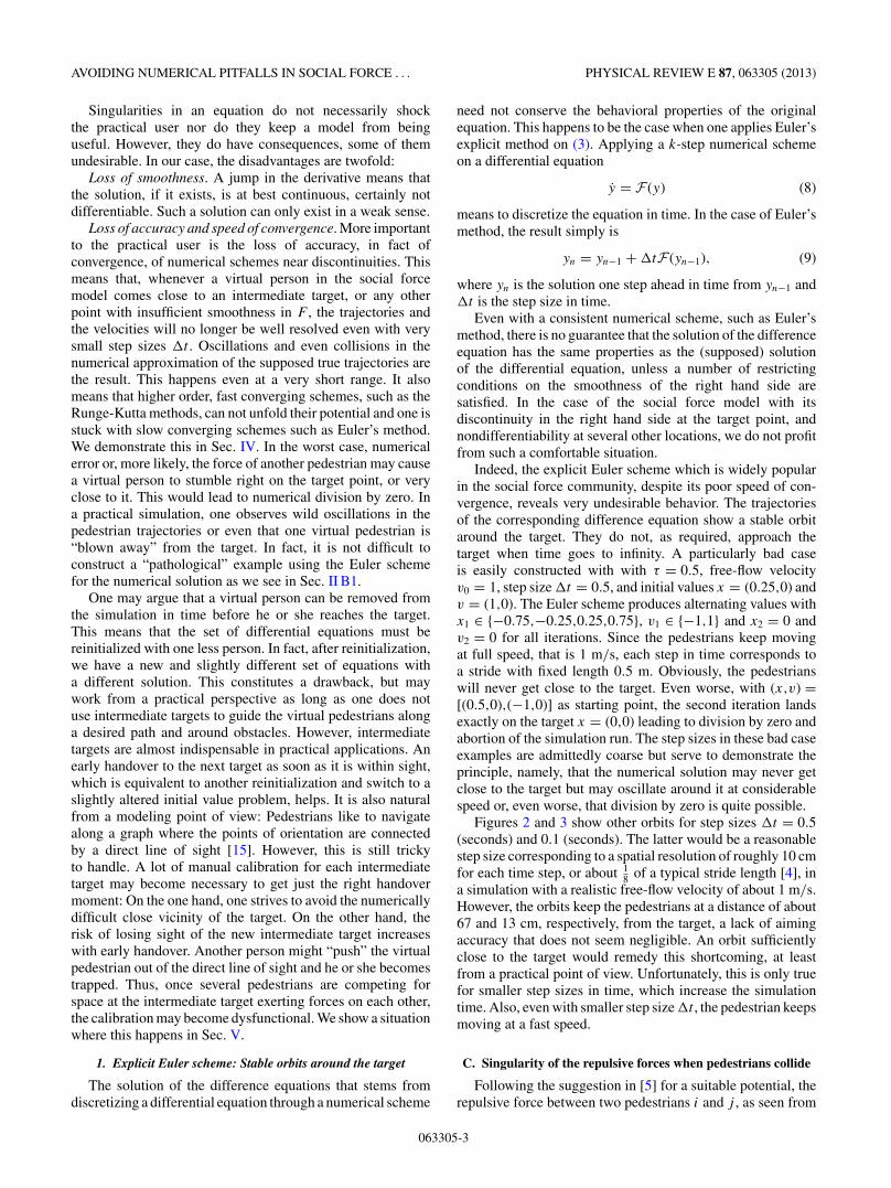
Figures 2 and 3 show other orbits for step sizes �t = 0.5(seconds) and 0.1 (seconds). The latter would be a reasonablestep size corresponding to a spatial resolution of roughly 10 cmfor each time step, or about 1
8 of a typical stride length [4], ina simulation with a realistic free-flow velocity of about 1 m/s.However, the orbits keep the pedestrians at a distance of about67 and 13 cm, respectively, from the target, a lack of aimingaccuracy that does not seem negligible. An orbit sufficientlyclose to the target would remedy this shortcoming, at leastfrom a practical point of view. Unfortunately, this is only truefor smaller step sizes in time, which increase the simulationtime. Also, even with smaller step size �t , the pedestrian keepsmoving at a fast speed.
C. Singularity of the repulsive forces when pedestrians collide
Following the suggestion in [5] for a suitable potential, therepulsive force between two pedestrians i and j , as seen from
063305-3
GERTA KOSTER, FRANZ TREML, AND MARION GODEL PHYSICAL REVIEW E 87, 063305 (2013)
0 5 10 15 20 25 300.2
0.4
0.6
0.8
1
1.2
1.4
1.6
time [s]
spee
d [m
/s] |
dis
tanc
e fr
om ta
rget
[m]
Solution behavior near the target − Euler, stepsize 0.5 s
speed [m/s]distance from target [m]
−1 −0.5 0 0.5 1 1.5−0.8
−0.6
−0.4
−0.2
0
0.2
0.4
0.6
0.8Solution trajectory − Euler, stepsize 0.5 s
x1
x 2
starting pointtargetpath
FIG. 2. (Color online) Euler’s scheme to solve the SFM develops a stable orbit around the target, never reaching the target and neverslowing down. With step size in time �t = 0.5 s and free-flow velocity 1.34 m/s, the person remains about 0.67 m off target and keeps movingat full speed.
pedestrian i, is given by
Fped,i,j = xi − xj
‖xi − xj‖V 0
σe− ‖xi−xj ‖
σ , (10)
where xi denotes the position of pedestrian i.For simplicity, we stick to a circular shape of the pedestri-
ans. Parameters V 0 and σ vary the strength and reach of theforce. Calibration should ensure that pedestrians do not overlapin standard situations. Unfortunately, this is a delicate task thathas yet to be completed to full satisfaction [8]. Calibration,however, is not the goal of this paper. So, we use the parameterchoices V 0 = 2.1 m2/s2 and σ = 0.3 m from [5] despitethe fact that we observe overlapping in simple situations(see Sec. IV).
The force contains the termxi − xj
‖xi − xj‖ (11)
that becomes singular whenever xi = xj . However, unlikebefore, there is no attraction pointing towards the singularity.Quite the contrary, the repulsive forces increase with decreas-ing distance between the torsos’ midpoints. Thus, only totalcollision would have a numerical impact on a simulation run.
D. Loss of differentiability at the desired speed
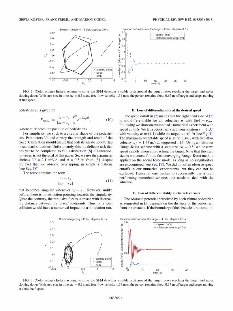
The speed cutoff in (2) means that the right hand side of (2)is not differentiable for all velocities w with ‖w‖ = vmax.Following we show an example of a numerical experiment withspeed cutoffs. We let a pedestrian start from position x = (1,0)with velocity w = (1,1) while the target is at (0,0) (see Fig. 4).The maximum acceptable speed is set to 1.3vi,0 with free-flowvelocity vi,0 = 1.34 m/s as suggested in [5]. Using a fifth orderRunge-Kutta scheme with a step size �t = 0.5, we observespeed cutoffs when approaching the target. Note that this stepsize is not coarse for the fast converging Runge-Kutta methodapplied on the social force model as long as no singularitiesare encountered (see Sec. IV). We did not often observe speedcutoffs in our numerical experiments, but they can not beexcluded. Hence, if one wishes to successfully use a highperforming numerical scheme, one needs to deal with thesituation.
E. Loss of differentiability at obstacle corners
The obstacle potential perceived by each virtual pedestrianas suggested in [5] depends on the distance of the pedestrianfrom the obstacle. If the boundary of the obstacle is not smooth,
0 10 20 30 400
0.5
1
1.5
time [s]
spee
d [m
/s] |
dis
tanc
e fr
om ta
rget
[m]
Solution behavior near the target − Euler, stepsize 0.1 s
speed [m/s]distance from target [m]
−0.5 0 0.5 1 1.5−0.2
−0.1
0
0.1
0.2
0.3
0.4
0.5Solution trajectory − Euler, stepsize 0.1 s
x1
x 2
starting pointtargetpath
FIG. 3. (Color online) Euler’s scheme to solve the SFM develops a stable orbit around the target, never reaching the target and neverslowing down. With step size in time �t = 0.1 s and free-flow velocity 1.34 m/s, the person remains about 0.13 m off target and keeps movingat about half speed.
063305-4
AVOIDING NUMERICAL PITFALLS IN SOCIAL FORCE . . . PHYSICAL REVIEW E 87, 063305 (2013)
0 2 4 6 8 100
2
4
6
8
10
12
time [s]
spee
d [m
/s]
before SCOafter SCO
0 2 4 6 8 10−1
0
1
2
time [s]
x 1
0 2 4 6 8 10−0.5
0
0.5
time [s]
x 2
no SCO
vmax = 1.742 m/s
no SCO
vmax = 1.742 m/s
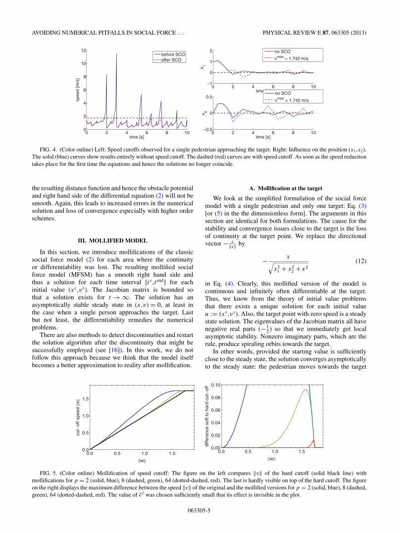
FIG. 4. (Color online) Left: Speed cutoffs observed for a single pedestrian approaching the target. Right: Influence on the position (x1,x2).The solid (blue) curves show results entirely without speed cutoff. The dashed (red) curves are with speed cutoff. As soon as the speed reductiontakes place for the first time the equations and hence the solutions no longer coincide.
the resulting distance function and hence the obstacle potentialand right hand side of the differential equation (2) will not besmooth. Again, this leads to increased errors in the numericalsolution and loss of convergence especially with higher orderschemes.
III. MOLLIFIED MODEL
In this section, we introduce mollifications of the classicsocial force model (2) for each area where the continuityor differentiability was lost. The resulting mollified socialforce model (MFSM) has a smooth right hand side andthus a solution for each time interval [t s,tend] for eachinitial value (xs,vs). The Jacobian matrix is bounded sothat a solution exists for t → ∞. The solution has anasymptotically stable steady state in (x,v) = 0, at least inthe case when a single person approaches the target. Lastbut not least, the differentiability remedies the numericalproblems.
There are also methods to detect discontinuities and restartthe solution algorithm after the discontinuity that might besuccessfully employed (see [16]). In this work, we do notfollow this approach because we think that the model itselfbecomes a better approximation to reality after mollification.
A. Mollification at the target
We look at the simplified formulation of the social forcemodel with a single pedestrian and only one target: Eq. (3)[or (5) in the the dimensionless form]. The arguments in thissection are identical for both formulations. The cause for thestability and convergence issues close to the target is the lossof continuity at the target point. We replace the directionalvector − x
‖x‖ by
− x√x2
1 + x22 + ε2
(12)
in Eq. (4). Clearly, this mollified version of the model iscontinuous and infinitely often differentiable at the target.Thus, we know from the theory of initial value problemsthat there exists a unique solution for each initial valueu := (xs,vs). Also, the target point with zero speed is a steadystate solution. The eigenvalues of the Jacobian matrix all havenegative real parts (− 1
2 ) so that we immediately get localasymptotic stability. Nonzero imaginary parts, which are therule, produce spiraling orbits towards the target.
In other words, provided the starting value is sufficientlyclose to the steady state, the solution converges asymptoticallyto the steady state: the pedestrian moves towards the target
0.0 0.5 1.0 1.50.00
0.02
0.04
0.06
0.08
0.10
w
diffe
renc
eso
ftto
hard
cut
off
0.0 0.5 1.0 1.50.0
0.5
1.0
1.5
w
cut
off
spee
dv
FIG. 5. (Color online) Mollification of speed cutoff: The figure on the left compares ‖v‖ of the hard cutoff (solid black line) withmollifications for p = 2 (solid, blue), 8 (dashed, green), 64 (dotted-dashed, red). The last is hardly visible on top of the hard cutoff. The figureon the right displays the maximum difference between the speed ‖v‖ of the original and the mollified versions for p = 2 (solid, blue), 8 (dashed,green), 64 (dotted-dashed, red). The value of ε2 was chosen sufficiently small that its effect is invisible in the plot.
063305-5
GERTA KOSTER, FRANZ TREML, AND MARION GODEL PHYSICAL REVIEW E 87, 063305 (2013)
2.0 1.5 1.0 0.5 0.0 0.5 1.0
1.0
0.5
0.0
0.5
1.0
1.5
2.0
x1
x 2
1.0 0.5 0.0 0.5 1.0 1.50.0
0.2
0.4
0.6
0.8
1.0
1.2
1.4
x2
dist
ance
toco
rner
for
x 10
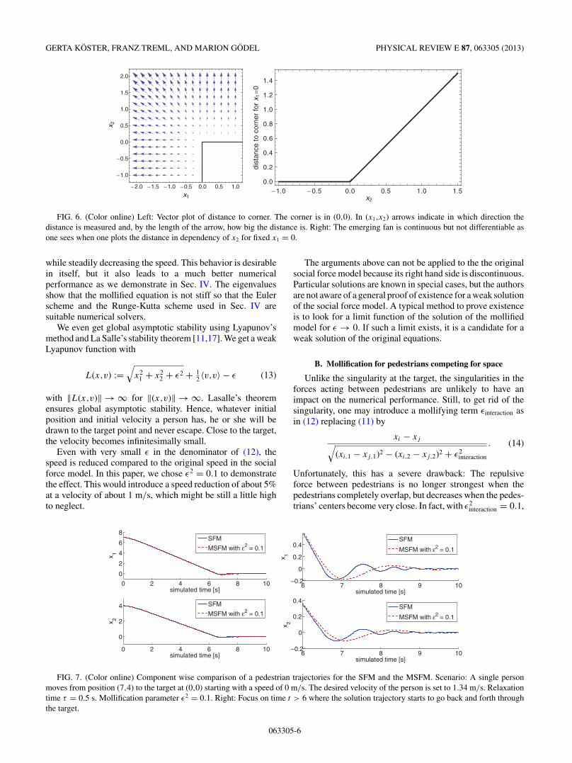
FIG. 6. (Color online) Left: Vector plot of distance to corner. The corner is in (0,0). In (x1,x2) arrows indicate in which direction thedistance is measured and, by the length of the arrow, how big the distance is. Right: The emerging fan is continuous but not differentiable asone sees when one plots the distance in dependency of x2 for fixed x1 = 0.
while steadily decreasing the speed. This behavior is desirablein itself, but it also leads to a much better numericalperformance as we demonstrate in Sec. IV. The eigenvaluesshow that the mollified equation is not stiff so that the Eulerscheme and the Runge-Kutta scheme used in Sec. IV aresuitable numerical solvers.
We even get global asymptotic stability using Lyapunov’smethod and La Salle’s stability theorem [11,17]. We get a weakLyapunov function with
L(x,v) :=√
x21 + x2
2 + ε2 + 12 〈v,v〉 − ε (13)
with ‖L(x,v)‖ → ∞ for ‖(x,v)‖ → ∞. Lasalle’s theoremensures global asymptotic stability. Hence, whatever initialposition and initial velocity a person has, he or she will bedrawn to the target point and never escape. Close to the target,the velocity becomes infinitesimally small.
Even with very small ε in the denominator of (12), thespeed is reduced compared to the original speed in the socialforce model. In this paper, we chose ε2 = 0.1 to demonstratethe effect. This would introduce a speed reduction of about 5%at a velocity of about 1 m/s, which might be still a little highto neglect.
The arguments above can not be applied to the the originalsocial force model because its right hand side is discontinuous.Particular solutions are known in special cases, but the authorsare not aware of a general proof of existence for a weak solutionof the social force model. A typical method to prove existenceis to look for a limit function of the solution of the mollifiedmodel for ε → 0. If such a limit exists, it is a candidate for aweak solution of the original equations.
B. Mollification for pedestrians competing for space
Unlike the singularity at the target, the singularities in theforces acting between pedestrians are unlikely to have animpact on the numerical performance. Still, to get rid of thesingularity, one may introduce a mollifying term εinteraction asin (12) replacing (11) by
xi − xj√(xi,1 − xj,1)2 − (xi,2 − xj,2)2 + ε2
interaction
. (14)
Unfortunately, this has a severe drawback: The repulsiveforce between pedestrians is no longer strongest when thepedestrians completely overlap, but decreases when the pedes-trians’ centers become very close. In fact, with ε2
interaction = 0.1,
0 2 4 6 8 10
0
2
4
6
8
simulated time [s]
x 1
SFM
MSFM with ε2 = 0.1
0 2 4 6 8 10
0
2
4
simulated time [s]
x 2
SFM
MSFM with ε2 = 0.1
6 7 8 9 10−0.2
0
0.2
0.4
simulated time [s]
x 1
6 7 8 9 10−0.2
0
0.2
0.4
simulated time [s]
x 2
SFM
MSFM with ε2 = 0.1
SFM
MSFM with ε2 = 0.1
FIG. 7. (Color online) Component wise comparison of a pedestrian trajectories for the SFM and the MSFM. Scenario: A single personmoves from position (7,4) to the target at (0,0) starting with a speed of 0 m/s. The desired velocity of the person is set to 1.34 m/s. Relaxationtime τ = 0.5 s. Mollification parameter ε2 = 0.1. Right: Focus on time t > 6 where the solution trajectory starts to go back and forth throughthe target.
063305-6
AVOIDING NUMERICAL PITFALLS IN SOCIAL FORCE . . . PHYSICAL REVIEW E 87, 063305 (2013)
6 7 8 9 100
0.1
0.2
0.3
0.4
0.5
0.6
0.7
0.8
simulated time [s]
dist
ance
to th
e ta
rget
[m]
SFM
MSFM with ε2 = 0.1
0 2 4 6 8 100
0.2
0.4
0.6
0.8
1
1.2
1.4
simulated time [s]
spee
d [m
/s]
SFM
MSFM with ε2 = 0.1desired speed
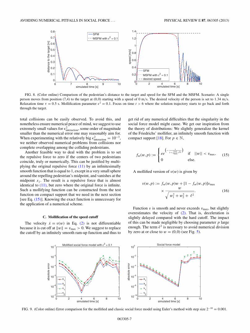
FIG. 8. (Color online) Comparison of the pedestrian’s distance to the target and speed for the SFM and the MSFM. Scenario: A singleperson moves from position (7,4) to the target at (0,0) starting with a speed of 0 m/s. The desired velocity of the person is set to 1.34 m/s.Relaxation time τ = 0.5 s. Mollification parameter ε2 = 0.1. Focus on time t > 6 where the solution trajectory starts to go back and forththrough the target.
total collisions can be easily observed. To avoid this, andnonetheless ensure numerical peace of mind, we suggest to useextremely small values for ε2
interaction, some order of magnitudesmaller than the numerical error one may reasonably aim for.When experimenting with the relatively big ε2
interaction = 10−3,we neither observed numerical problems from collisions norcomplete overlapping among the colliding pedestrians.
Another feasible way to deal with the problem is to setthe repulsive force to zero if the centers of two pedestrianscoincide, truly or numerically. This can be justified by multi-plying the original repulsive force (11) by an infinitesimallysmooth function that is equal to 1, except in a very small spherearound the repelling pedestrian’s midpoint, and vanishes at themidpoint xj . The result is a repulsive force that is almostidentical to (11), but zero where the original force is infinite.Such a mollifying function can be constructed from the testfunction on compact support that we need in the next section[see Eq. (15)]. Knowing the exact function is unnecessary forthe application of a numerical scheme.
C. Mollification of the speed cutoff
The velocity x = v(w) in Eq. (2) is not differentiablebecause it is cut off at ‖w‖ = vmax > 0. We suggest to replacethe cutoff by an infinitely smooth ram-up function and thus to
get rid of any numerical difficulties that the singularity in thesocial force model might cause. We get our inspiration fromthe theory of distributions: We slightly generalize the kernelof the Friedrichs’ mollifier, an infinitely smooth function withcompact support [18]. For p ∈ N,
fm(w,p) :=⎧⎨⎩ ee
(− 1
1−( ‖w‖vmax )2p
)if ||w|| < vmax,
0 else.(15)
A mollified version of v(w) is given by
v(w,p) := fm(w,p)w + [1 − fm(w,p)]vmax
× w√w2
1 + w22 + ε2
. (16)
Function v is smooth and never exceeds vmax, but slightlyoverestimates the velocity of (2). That is, deceleration isslightly delayed compared with the hard cutoff. The impactof this can be made negligible by choosing parameter p largeenough. The term ε2 is necessary to avoid numerical divisionby zero at or close to w = (0,0) (see Fig. 5).
0 2 4 6 8 1010
−7
10−6
10−5
10−4
10−3
10−2
simulated time [s]
abso
lute
err
or
Mollified social force model with ε2 = 0.1
x1
x2
v1
v2
0 2 4 6 8 1010
−10
10−8
10−6
10−4
10−2
100
simulated time [s]
abso
lute
err
or
Social force model
x1
x2
v1
v2
FIG. 9. (Color online) Error comparison for the mollified and classic social force model using Euler’s method with step size 2−10 = 0.001.
063305-7
GERTA KOSTER, FRANZ TREML, AND MARION GODEL PHYSICAL REVIEW E 87, 063305 (2013)
0 2 4 6 8 1010
−8
10−6
10−4
10−2
100
simulated time [s]
abso
lute
err
or
Mollified social force model with ε2 = 0.1
x1
x2
v1
v2
0 2 4 6 8 1010
−8
10−6
10−4
10−2
100
simulated time [s]
abso
lute
err
or
Social force model
x1
x2
v1
v2
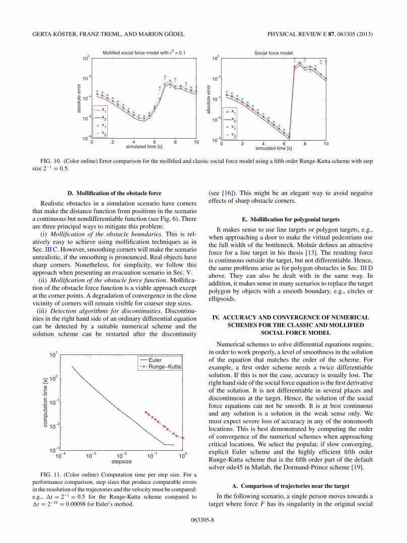
FIG. 10. (Color online) Error comparison for the mollified and classic social force model using a fifth order Runge-Kutta scheme with stepsize 2−1 = 0.5.
D. Mollification of the obstacle force
Realistic obstacles in a simulation scenario have cornersthat make the distance function from positions in the scenarioa continuous but nondifferentiable function (see Fig. 6). Thereare three principal ways to mitigate this problem:
(i) Mollification of the obstacle boundaries. This is rel-atively easy to achieve using mollification techniques as inSec. III C. However, smoothing corners will make the scenariounrealistic, if the smoothing is pronounced. Real objects havesharp corners. Nonetheless, for simplicity, we follow thisapproach when presenting an evacuation scenario in Sec. V.
(ii) Mollification of the obstacle force function. Mollifica-tion of the obstacle force function is a viable approach exceptat the corner points. A degradation of convergence in the closevicinity of corners will remain visible for coarser step sizes.
(iii) Detection algorithms for discontinuities. Discontinu-ities in the right hand side of an ordinary differential equationcan be detected by a suitable numerical scheme and thesolution scheme can be restarted after the discontinuity
10−4
10−3
10−2
10−1
100
10−3
10−2
10−1
100
101
stepsize
com
puta
tion
time
[s]
EulerRunge−Kutta
FIG. 11. (Color online) Computation time per step size. For aperformance comparison, step sizes that produce comparable errorsin the resolution of the trajectories and the velocity must be compared:e.g., �t = 2−1 = 0.5 for the Runge-Kutta scheme compared to�t = 2−10 = 0.00098 for Euler’s method.
(see [16]). This might be an elegant way to avoid negativeeffects of sharp obstacle corners.
E. Mollification for polygonial targets
It makes sense to use line targets or polygon targets, e.g.,when approaching a door to make the virtual pedestrians usethe full width of the bottleneck. Molnar defines an attractiveforce for a line target in his thesis [13]. The resulting forceis continuous outside the target, but not differentiable. Hence,the same problems arise as for polygon obstacles in Sec. III Dabove. They can also be dealt with in the same way. Inaddition, it makes sense in many scenarios to replace the targetpolygon by objects with a smooth boundary, e.g., circles orellipsoids.
IV. ACCURACY AND CONVERGENCE OF NUMERICALSCHEMES FOR THE CLASSIC AND MOLLIFIED
SOCIAL FORCE MODEL
Numerical schemes to solve differential equations require,in order to work properly, a level of smoothness in the solutionof the equation that matches the order of the scheme. Forexample, a first order scheme needs a twice differentiablesolution. If this is not the case, accuracy is usually lost. Theright hand side of the social force equation is the first derivativeof the solution. It is not differentiable in several places anddiscontinuous at the target. Hence, the solution of the socialforce equations can not be smooth. It is at best continuousand any solution is a solution in the weak sense only. Wemust expect severe loss of accuracy in any of the nonsmoothlocations. This is best demonstrated by computing the orderof convergence of the numerical schemes when approachingcritical locations. We select the popular, if slow converging,explicit Euler scheme and the highly efficient fifth orderRunge-Kutta scheme that is the fifth order part of the defaultsolver ode45 in Matlab, the Dormand-Prince scheme [19].
A. Comparison of trajectories near the target
In the following scenario, a single person moves towards atarget where force F has its singularity in the original social
063305-8
AVOIDING NUMERICAL PITFALLS IN SOCIAL FORCE . . . PHYSICAL REVIEW E 87, 063305 (2013)
10−5
10−4
10−3
10−2
10−1
1000.99
1
1.01
1.02
1.03
1.04
1.05
1.06
stepsize
orde
r of
con
verg
ence
Mollified social force model with ε2 = 0.1
x1
x2
v1
v2
10−5
10−4
10−3
10−2
10−1
10010
−6
10−5
10−4
10−3
10−2
10−1
stepsize
abso
lute
err
or a
t t =
1
Mollified social force model with ε2 = 0.1
x1
x2
v1
v2
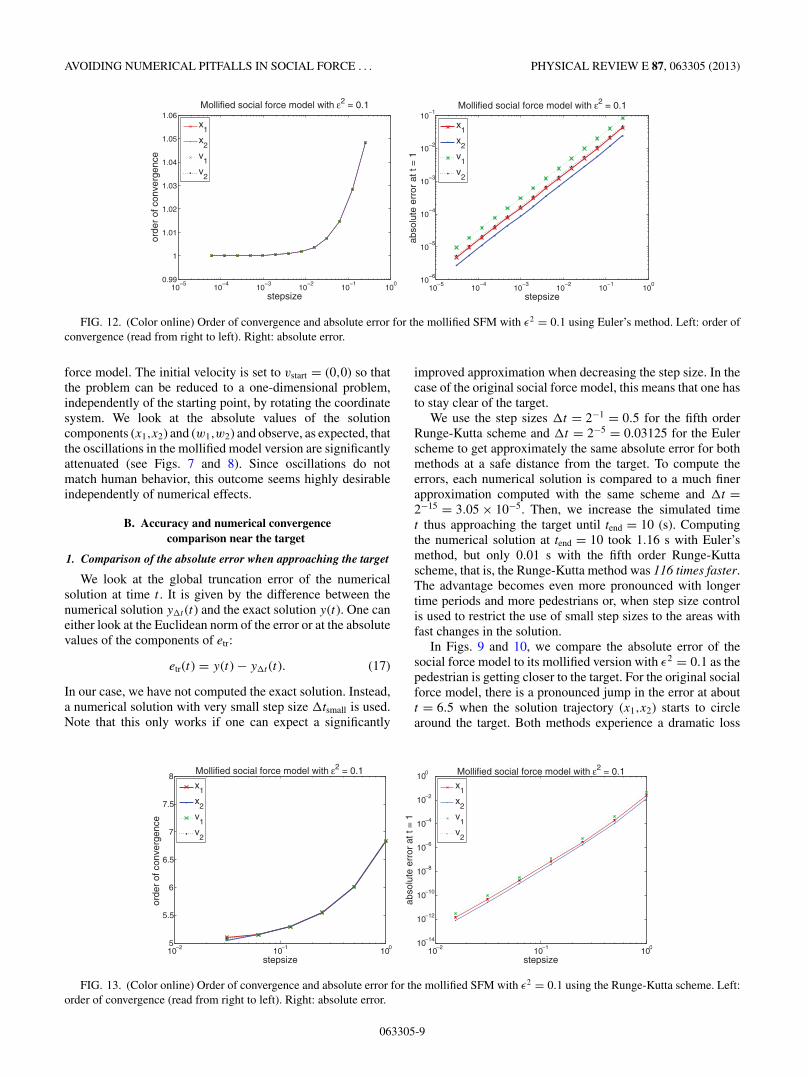
FIG. 12. (Color online) Order of convergence and absolute error for the mollified SFM with ε2 = 0.1 using Euler’s method. Left: order ofconvergence (read from right to left). Right: absolute error.
force model. The initial velocity is set to vstart = (0,0) so thatthe problem can be reduced to a one-dimensional problem,independently of the starting point, by rotating the coordinatesystem. We look at the absolute values of the solutioncomponents (x1,x2) and (w1,w2) and observe, as expected, thatthe oscillations in the mollified model version are significantlyattenuated (see Figs. 7 and 8). Since oscillations do notmatch human behavior, this outcome seems highly desirableindependently of numerical effects.
B. Accuracy and numerical convergencecomparison near the target
1. Comparison of the absolute error when approaching the target
We look at the global truncation error of the numericalsolution at time t . It is given by the difference between thenumerical solution y�t (t) and the exact solution y(t). One caneither look at the Euclidean norm of the error or at the absolutevalues of the components of etr:
etr(t) = y(t) − y�t (t). (17)
In our case, we have not computed the exact solution. Instead,a numerical solution with very small step size �tsmall is used.Note that this only works if one can expect a significantly
improved approximation when decreasing the step size. In thecase of the original social force model, this means that one hasto stay clear of the target.
We use the step sizes �t = 2−1 = 0.5 for the fifth orderRunge-Kutta scheme and �t = 2−5 = 0.03125 for the Eulerscheme to get approximately the same absolute error for bothmethods at a safe distance from the target. To compute theerrors, each numerical solution is compared to a much finerapproximation computed with the same scheme and �t =2−15 = 3.05 × 10⁻⁵. Then, we increase the simulated timet thus approaching the target until tend = 10 (s). Computingthe numerical solution at tend = 10 took 1.16 s with Euler’smethod, but only 0.01 s with the fifth order Runge-Kuttascheme, that is, the Runge-Kutta method was 116 times faster.The advantage becomes even more pronounced with longertime periods and more pedestrians or, when step size controlis used to restrict the use of small step sizes to the areas withfast changes in the solution.
In Figs. 9 and 10, we compare the absolute error of thesocial force model to its mollified version with ε2 = 0.1 as thepedestrian is getting closer to the target. For the original socialforce model, there is a pronounced jump in the error at aboutt = 6.5 when the solution trajectory (x1,x2) starts to circlearound the target. Both methods experience a dramatic loss
10−2 10−1 1005
5.5
6
6.5
7
7.5
8
stepsize
orde
r of
con
verg
ence
Mollified social force model with ε2 = 0.1
x1
x2
v1
v2
10−2 10−1 10010−14
10−12
10−10
10−8
10−6
10−4
10−2
100
stepsize
abso
lute
err
or a
t t =
1
Mollified social force model with ε2 = 0.1
x1
x2
v1
v2
FIG. 13. (Color online) Order of convergence and absolute error for the mollified SFM with ε2 = 0.1 using the Runge-Kutta scheme. Left:order of convergence (read from right to left). Right: absolute error.
063305-9
GERTA KOSTER, FRANZ TREML, AND MARION GODEL PHYSICAL REVIEW E 87, 063305 (2013)
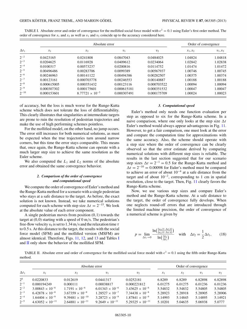
TABLE I. Absolute error and order of convergence for the mollified social force model with ε2 = 0.1 using Euler’s first order method. Theorder of convergence for x1 and x2 as well as v1 and v2 coincide up to the accuracy considered here.
Absolute error Order of convergence
�t1 x1 x2 v1 v2 x1,x2 v1,v2
2−2 0.0423165 0.0241808 0.0847043 0.0484025 1.04824 1.048182−3 0.0204625 0.0116928 0.0409612 0.0234064 1.02842 1.028382−4 0.0100317 0.00573237 0.0200816 0.0114752 1.01474 1.014722−5 0.00496486 0.00283706 0.0099389 0.00567937 1.00746 1.007452−6 0.00246963 0.00141122 0.00494386 0.00282507 1.00375 1.003742−7 0.00123161 0.000703778 0.00246553 0.00140887 1.00188 1.001882−8 0.000615005 0.000351432 0.00123116 0.000703522 1.00094 1.000942−9 0.000307302 0.000175601 0.000615181 0.000351532 1.00047 1.000472−10 0.000153601 8.77721 × 10⁻⁵ 0.000307491 0.000175709 1.00024 1.00023
of accuracy, but the loss is much worse for the Runge-Kuttascheme which does not tolerate the loss of differentiability.This clearly illustrates that singularities at intermediate targetsare prone to ruin the resolution of pedestrian trajectories andmake the use of high performing schemes pointless.
For the mollified model, on the other hand, no jump occurs.The error still increases for both numerical solutions, as mustbe expected when the true trajectories turn around narrowcorners, but this time the error stays comparable. This meansthat, once again, the Runge-Kutta scheme can operate with amuch larger step size to achieve the same resolution as theEuler scheme.
We also computed the L1 and L2 norms of the absoluteerror and obtained the same convergence behavior.
2. Comparison of the order of convergenceand computational speed
We compute the order of convergence of Euler’s method andthe Runge-Kutta method for a scenario with a single pedestrianwho stays at a safe distance to the target. As before, the exactsolution is not known. Instead, we take numerical solutionscomputed for each scheme with step size �t = 2−15. We lookat the absolute value of each error component.
A single pedestrian moves from position (0,1) towards thetarget at (0,0) starting with a speed of 0 m/s. The pedestrian’sfree-flow velocity v0 is set to 1.34 m/s and the relaxation time τ
to 0.5 s. At this distance to the target, the results with the socialforce model (SFM) and the mollified version (MSFM) arealmost identical. Therefore, Figs. 11, 12, and 13 and Tables Iand II only show the behavior of the mollified SFM.
3. Computational speed
Euler’s method only needs one function evaluation perstep as opposed to six for the Runge-Kutta scheme. In anaive comparison, where one only looks at the step size �t
Euler’s method would always appear advantageous in Fig. 11.However, to get a fair comparison, one must look at the errorand compare the computation time for approximations withthe same accuracy. Also, the scheme should operate witha step size where the order of convergence can be clearlyobserved so that the error estimate derived by comparingnumerical solutions with different step sizes is reliable. Theresults in the last section suggested that for our scenariostep sizes �t = 2−1 = 0.5 for the Runge-Kutta method and�t = 2−10 = 0.00098 for Euler’s method must be comparedto achieve an error of about 10−4 at a safe distance from thetarget and of about 10−2, corresponding to 1 cm in spatialresolution, close to the target. Then, Fig. 11 clearly favors theRunge-Kutta scheme.
Now, we use various step sizes and compare Euler’smethod and the Runge-Kutta scheme. At a safe distance tothe target, the order of convergence fully develops. Whenone neglects round-off errors that are introduced throughthe limited machine precision, the order of convergence ofa numerical scheme is given by
p = lim�t1→0
ln( ‖etr(y,�t2)‖
‖etr(y,�t1)‖)
ln(
�t2�t1
) with �t2 = 1
2�t1, (18)
TABLE II. Absolute error and order of convergence for the mollified social force model with ε2 = 0.1 using the fifth order Runge-Kuttamethod.
Absolute error Order of convergence
�t1 x1 x2 v1 v2 x1 x2 v1 v2
20 0.0220833 0.012619 0.0441317 0.0252181 6.8289 6.8289 6.82898 6.828982−1 0.000194249 0.000111 0.00038817 0.000221812 6.01275 6.01275 6.01236 6.012362−2 3.00843 × 10⁻⁶ 1.7191 × 10⁻⁶ 6.01343 × 10⁻⁶ 3.43625 × 10⁻⁶ 5.54832 5.54832 5.54805 5.548052−3 6.42878 × 10⁻⁸ 3.67359 × 10⁻⁸ 1.28527 × 10⁻⁷ 7.34438 × 10⁻⁸ 5.28923 5.28918 5.28905 5.289062−4 1.64404 × 10⁻⁹ 9.39481 × 10⁻¹⁰ 3.28723 × 10⁻⁹ 1.87841 × 10⁻⁹ 5.14993 5.14845 5.14895 5.149212−5 4.63052 × 10⁻¹¹ 2.64881 × 10⁻¹¹ 9.2649 × 10⁻¹¹ 5.29325 × 10⁻¹¹ 5.10201 5.04635 5.06938 5.0777
063305-10
AVOIDING NUMERICAL PITFALLS IN SOCIAL FORCE . . . PHYSICAL REVIEW E 87, 063305 (2013)
−1 −0.5 0 0.5 1−1
−0.5
0
0.5
1
1.5
x1
x 2
pedestrian 1pedestrian 2
−1 −0.5 0 0.5 1−1
−0.5
0
0.5
1
1.5
x1
x 2
pedestrian 1pedestrian 2
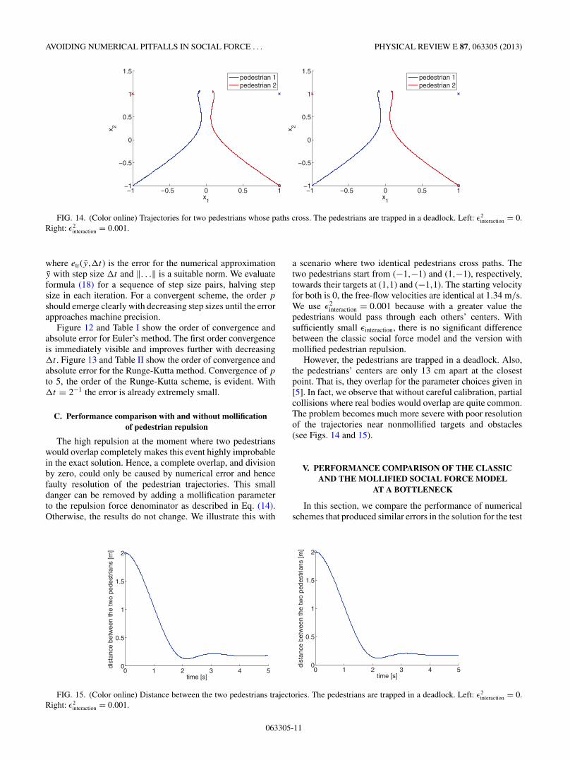
FIG. 14. (Color online) Trajectories for two pedestrians whose paths cross. The pedestrians are trapped in a deadlock. Left: ε2interaction = 0.
Right: ε2interaction = 0.001.
where etr(y,�t) is the error for the numerical approximationy with step size �t and ‖. . .‖ is a suitable norm. We evaluateformula (18) for a sequence of step size pairs, halving stepsize in each iteration. For a convergent scheme, the order p
should emerge clearly with decreasing step sizes until the errorapproaches machine precision.
Figure 12 and Table I show the order of convergence andabsolute error for Euler’s method. The first order convergenceis immediately visible and improves further with decreasing�t . Figure 13 and Table II show the order of convergence andabsolute error for the Runge-Kutta method. Convergence of p
to 5, the order of the Runge-Kutta scheme, is evident. With�t = 2−1 the error is already extremely small.
C. Performance comparison with and without mollificationof pedestrian repulsion
The high repulsion at the moment where two pedestrianswould overlap completely makes this event highly improbablein the exact solution. Hence, a complete overlap, and divisionby zero, could only be caused by numerical error and hencefaulty resolution of the pedestrian trajectories. This smalldanger can be removed by adding a mollification parameterto the repulsion force denominator as described in Eq. (14).Otherwise, the results do not change. We illustrate this with
a scenario where two identical pedestrians cross paths. Thetwo pedestrians start from (−1,−1) and (1,−1), respectively,towards their targets at (1,1) and (−1,1). The starting velocityfor both is 0, the free-flow velocities are identical at 1.34 m/s.We use ε2
interaction = 0.001 because with a greater value thepedestrians would pass through each others’ centers. Withsufficiently small εinteraction, there is no significant differencebetween the classic social force model and the version withmollified pedestrian repulsion.
However, the pedestrians are trapped in a deadlock. Also,the pedestrians’ centers are only 13 cm apart at the closestpoint. That is, they overlap for the parameter choices given in[5]. In fact, we observe that without careful calibration, partialcollisions where real bodies would overlap are quite common.The problem becomes much more severe with poor resolutionof the trajectories near nonmollified targets and obstacles(see Figs. 14 and 15).
V. PERFORMANCE COMPARISON OF THE CLASSICAND THE MOLLIFIED SOCIAL FORCE MODEL
AT A BOTTLENECK
In this section, we compare the performance of numericalschemes that produced similar errors in the solution for the test
0 1 2 3 4 50
0.5
1
1.5
2
time [s]
dist
ance
bet
wee
n th
e tw
o pe
dest
rians
[m]
0 1 2 3 4 50
0.5
1
1.5
2
time [s]
dist
ance
bet
wee
n th
e tw
o pe
dest
rians
[m]
FIG. 15. (Color online) Distance between the two pedestrians trajectories. The pedestrians are trapped in a deadlock. Left: ε2interaction = 0.
Right: ε2interaction = 0.001.
063305-11
GERTA KOSTER, FRANZ TREML, AND MARION GODEL PHYSICAL REVIEW E 87, 063305 (2013)
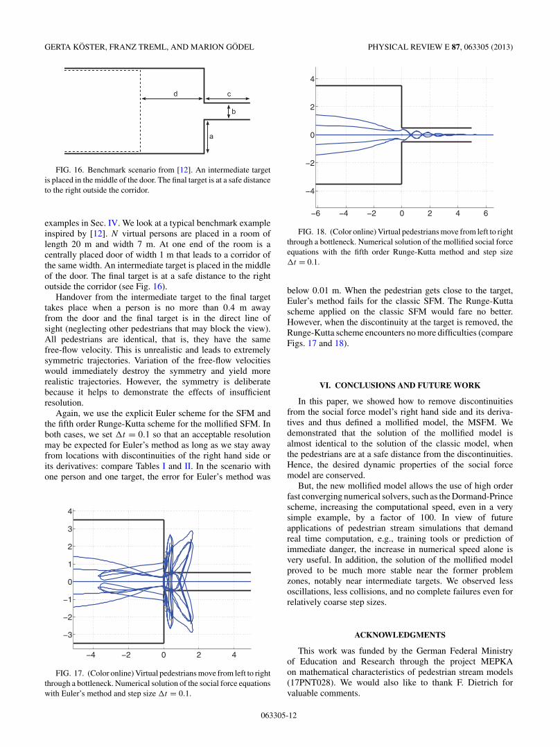
FIG. 16. Benchmark scenario from [12]. An intermediate targetis placed in the middle of the door. The final target is at a safe distanceto the right outside the corridor.
examples in Sec. IV. We look at a typical benchmark exampleinspired by [12]. N virtual persons are placed in a room oflength 20 m and width 7 m. At one end of the room is acentrally placed door of width 1 m that leads to a corridor ofthe same width. An intermediate target is placed in the middleof the door. The final target is at a safe distance to the rightoutside the corridor (see Fig. 16).
Handover from the intermediate target to the final targettakes place when a person is no more than 0.4 m awayfrom the door and the final target is in the direct line ofsight (neglecting other pedestrians that may block the view).All pedestrians are identical, that is, they have the samefree-flow velocity. This is unrealistic and leads to extremelysymmetric trajectories. Variation of the free-flow velocitieswould immediately destroy the symmetry and yield morerealistic trajectories. However, the symmetry is deliberatebecause it helps to demonstrate the effects of insufficientresolution.
Again, we use the explicit Euler scheme for the SFM andthe fifth order Runge-Kutta scheme for the mollified SFM. Inboth cases, we set �t = 0.1 so that an acceptable resolutionmay be expected for Euler’s method as long as we stay awayfrom locations with discontinuities of the right hand side orits derivatives: compare Tables I and II. In the scenario withone person and one target, the error for Euler’s method was
−4 −2 0 2 4
−3
−2
−1
0
1
2
3
4
FIG. 17. (Color online) Virtual pedestrians move from left to rightthrough a bottleneck. Numerical solution of the social force equationswith Euler’s method and step size �t = 0.1.
−6 −4 −2 0 2 4 6
−4
−2
0
2
4
FIG. 18. (Color online) Virtual pedestrians move from left to rightthrough a bottleneck. Numerical solution of the mollified social forceequations with the fifth order Runge-Kutta method and step size�t = 0.1.
below 0.01 m. When the pedestrian gets close to the target,Euler’s method fails for the classic SFM. The Runge-Kuttascheme applied on the classic SFM would fare no better.However, when the discontinuity at the target is removed, theRunge-Kutta scheme encounters no more difficulties (compareFigs. 17 and 18).
VI. CONCLUSIONS AND FUTURE WORK
In this paper, we showed how to remove discontinuitiesfrom the social force model’s right hand side and its deriva-tives and thus defined a mollified model, the MSFM. Wedemonstrated that the solution of the mollified model isalmost identical to the solution of the classic model, whenthe pedestrians are at a safe distance from the discontinuities.Hence, the desired dynamic properties of the social forcemodel are conserved.
But, the new mollified model allows the use of high orderfast converging numerical solvers, such as the Dormand-Princescheme, increasing the computational speed, even in a verysimple example, by a factor of 100. In view of futureapplications of pedestrian stream simulations that demandreal time computation, e.g., training tools or prediction ofimmediate danger, the increase in numerical speed alone isvery useful. In addition, the solution of the mollified modelproved to be much more stable near the former problemzones, notably near intermediate targets. We observed lessoscillations, less collisions, and no complete failures even forrelatively coarse step sizes.
ACKNOWLEDGMENTS
This work was funded by the German Federal Ministryof Education and Research through the project MEPKAon mathematical characteristics of pedestrian stream models(17PNT028). We would also like to thank F. Dietrich forvaluable comments.
063305-12
AVOIDING NUMERICAL PITFALLS IN SOCIAL FORCE . . . PHYSICAL REVIEW E 87, 063305 (2013)
[1] S. Gwynne, E. Galea, M. Owen, P. Lawrence, and L. Filippidis,Build. Environ. 34, 741 (1999).
[2] X. Zheng, T. Zhong, and M. Liu, Build. Environ. 44, 437 (2009).[3] A. Smith, C. James, R. Jones, P. Langston, E. Lester, and
J. Drury, Safety Sci. 47, 395 (2009).[4] M. J. Seitz and G. Koster, Phys. Rev. E 86, 046108 (2012).[5] D. Helbing and P. Molnar, Phys. Rev. E 51, 4282 (1995).[6] D. Helbing, I. Farkas, and T. Vicsek, Nature (London) 407, 487
(2000).[7] M. Chraibi, A. Seyfried, and A. Schadschneider, Phys. Rev. E
82, 046111 (2010).[8] M. Chraibi, U. Kemloh, A. Schadschneider, and A. Seyfried,
Networks Heterogeneous Media 6, 425 (2011).[9] B. A. Schlake, Diplomarbeit thesis, Institut fur Numerische und
Angewandte Mathematik, Universitat Munster, 2008.[10] M. Griebel, S. Knapek, G. Zumbusch, and A. Caglar,
Numerische Simulation in der Molekuldynamik (Springer,Berlin, 2004).
[11] A. M. Stuart and A. R. Humphries, in Dynamical Systems andNumerical Analysis, edited by P. Ciarlet, A. Iserles, R. Kohn,
and M. H. Wright (Cambridge University Press, Cambridge,UK, 1996).
[12] J. Liddle, A. Seyfried, and S. Boltes, in Pedestrian and Evacua-tion Dynamics, edited by R. D. Peacock, E. D. Kuligowski, andJ. D. Averill (Springer, Berlin, 2011), pp. 833–836.
[13] P. Molnar, Ph.D. thesis, Universitat Stuttgart, 1996.[14] U. Weidmann, Transporttechnik der Fussganger, 2nd ed.,
Schriftenreihe des IVT, Vol. 90 (Institut fur Verkehrsplanung,Zurich, 1992).
[15] A. Kneidl, Ph.D. thesis, Methoden zur Abbildung men-schlichen Navigationsverhaltens bei der Modellierung vonFußgangerstromen, 2013.
[16] E. Eich-Soellner, Ph.D. thesis, Universitat Augsburg, 1991.[17] J. L. Salle and S. Lefschetz, in Stability by Liapunov’s Direct
Method-With Applications, edited by R. Bellmann (Academic,New York, 1961).
[18] L. C. Evans, in Partial Differential Equations (AmericanMathematical Society, Providence, RI, 1997), p. 664.
[19] J. Dormand and P. Prince, J. Comput. Appl. Math. 6, 19(1980).
063305-13