Axions and ALPs: a very short introduction

David J. E. Marsh1,2

1Department of Physics, King’s College London, United Kingdom.2Institut fur Astrophysik, Georg-August Universitat, Gottingen, Germany.

The QCD axion was originally predicted as a dynamical solution to the strong CP problem.Axion like particles (ALPs) are also a generic prediction of many high energy physicsmodels including string theory. Theoretical models for axions are reviewed, giving a genericmulti-axion action with couplings to the standard model. The couplings and masses ofthese axions can span many orders of magnitude, and cosmology leads us to considerseveral distinct populations of axions behaving as coherent condensates, or relativisticparticles. Light, stable axions are a mainstay dark matter candidate. Axion cosmologyand calculation of the relic density are reviewed. A very brief survey is given of thephenomenology of axions arising from their direct couplings to the standard model, andtheir distinctive gravitational interactions.

1 Theory of Axions

1.1 The QCD Axion

The QCD axion was introduced by Peccei & Quinn [1], Weinberg [2], and Wilczek [3] (PQWW)in 1977-78 as a solution to the CP problem of the strong interaction. This arises from theChern-Simons term:

LθQCD =θQCD

32π2Tr GµνG

µν , (1)

where G is the gluon field strength tensor, Gµν = εαβµνGαβ is the dual, and the trace runsover the colour SU(3) indices. This term is called topological since it is a total derivative anddoes not affect the classical equations of motion. However, it has important effects on thequantum theory. This term is odd under CP, and so produces CP-violating interactions, suchas a neutron electric dipole moment (EDM), dn. The value of dn produced by this term wascomputed in Ref. [4] to be

dn ≈ 3.6× 10−16θQCD e cm , (2)

where e is the charge on the electron. The (permanent, static) dipole moment is constrainedto |dn| < 3.0× 10−26 e cm (90% C.L.) [5], implying θQCD . 10−10.

If there were only the CP-conserving strong interactions, then θQCD could simply be setto zero by symmetry. In the real world, and very importantly, the weak interactions violateCP [6]. By chiral rotations of the quark fields, we see that the physically measurable parameteris

θQCD = θQCD + arg detMuMd , (3)

Patras 2017 1

arX

iv:1

712.

0301

8v1

[he

p-ph

] 8

Dec

201

7

where θ is the “bare” (i.e. pure QCD) quantity and Mu, Md are the quark mass matrices. Thusthe smallness of θQCD implied by the EDM constraint is a fine tuning problem since it involvesa precise cancellation between two dimensionless terms generated by different physics.

The famous PQ solution to this relies on two ingredients: the Goldstone theorem, and thepresence of instantons in the QCD vacuum. A global chiral U(1)PQ symmetry, is introduced,under which some quarks are charged. This symmetry is spontaneously broken by a scalar field.More precisely, the symmetry breaking potential for the complex scalar ϕ is:

V (ϕ) = λ(|ϕ|2 − f2a/2)2 ⇒ 〈ϕ〉 = (fa/

√2)eiφ/fa . (4)

The Goldstone boson is φ, the axion, and I have defined the vacuum expectation value (VEV) ofthe field to be fa/

√2 to give canonical kinetic terms. fa is known as the axion “decay constant”

(we will shortly see the analogy to pions).The charges, QPQ of some quarks (either the standard model quarks or new heavy objects

with colour charge) under U(1)PQ are such that the PQ symmetry is anomalous, with the colouranomaly given by [7]:

Cδab = 2Tr QPQTaTb . (5)

The trace is over all the quarks, and the Ta are the generators for the representations of thequarks under SU(3). An anomalous chiral rotation by φ/fa of the quarks changes the fermionmeasure in the path integral, and leads to a change in the action:

S → S +

∫d4x

C32π2

φ

faTrGµνG

µν . (6)

For the QCD axion it is common to absorb the colour anomaly into the definition of fa, and keepthe VEV a separate quantity vPQ. However, I find it more useful, especially when consideringmulti-axion theories, to keep the anomaly factors explicit.

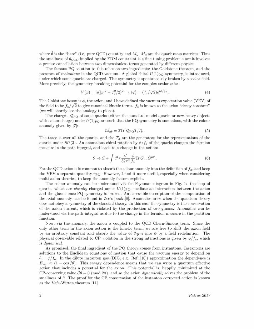
The colour anomaly can be understood via the Feynman diagram in Fig. 1: the loop ofquarks, which are chirally charged under U(1)PQ, mediate an interaction between the axionand the gluons once PQ symmetry is broken. An accessible description of the computation ofthe axial anomaly can be found in Zee’s book [8]. Anomalies arise when the quantum theorydoes not obey a symmetry of the classical theory. In this case the symmetry is the conservationof the axion current, which is violated by the production of two gluons. Anomalies can beunderstood via the path integral as due to the change in the fermion measure in the partitionfunction.

Now, via the anomaly, the axion is coupled to the QCD Chern-Simons term. Since theonly other term in the axion action is the kinetic term, we are free to shift the axion fieldby an arbitrary constant and absorb the value of θQCD into φ by a field redefinition. Thephysical observable related to CP violation in the strong interactions is given by φ/fa, whichis dynamical.

As promised, the final ingredient of the PQ theory comes from instantons. Instantons aresolutions to the Euclidean equations of motion that cause the vacuum energy to depend onθ = φ/fa. In the dilute instanton gas (DIG, e.g. Ref. [10]) approximation the dependence isEvac ∝ (1 − cos Cθ). This energy dependence means that we can write a quantum effectiveaction that includes a potential for the axion. This potential is, happily, minimized at theCP-conserving value Cθ = 0 (mod 2π), and so the axion dynamically solves the problem of thesmallness of θ. The proof for the CP conservation of the instanton corrected action is knownas the Vafa-Witten theorem [11].

2 Patras 2017

qµ

g

g

g

g

1/faq2 m2

Q

Q

Q

Q

Figure 1: The colour anomaly in the KSVZ axion model. Heavy quarks, Q, run in a loop withmomentum qµ. At low-momentum transfer, q2 m2

Q, the interaction can be replaced with the

effective φGG/fa interaction. Reproduced from Ref. [9].

The axion mass induced by the interaction with QCD was famously computed by Wein-berg [2] and Wilczek [3] using chiral perturbation theory (ChPT):

ma,QCD ≈ 6× 10−6 eV1012 GeV

fa/C, (7)

with the full ChPT potential at zero temperature given by (e.g. Ref. [12])

V (φ) = −m2πf

2π

√1− 4z sin2(Cφ/2fa) ; z =

mumd

(mu +md)2. (8)

Note that this potential differs from the DIG result, V (φ) ∝ cos(φ/fa), and that it vanishes inthe limit of massless quarks.1

The temperature dependence of the axion potential is expressed through the topologicalsusceptibilty of QCD, χ(T ). The axion potential is V (φ) = χ(T )U(θ) where T is temperatureand U(θ) is a dimensionless periodic function. Using that U(θ) is quadratic about the mini-mum for a massive particle we see that χ(T ) = m2

a(T )f2a , and so we often talk instead of the

temperature dependence of the axion mass. It is common to parameterise the dependence bya (possibly varying) power law: :

ma(T ) = ma,0

(T

ΛQCD

)−n

; (T ΛQCD) , (9)

with the mass approaching the zero temperature value for T < ΛQCD. At lowest order the DIGgives the famous result n = 4 for QCD in the standard model [13].2 In the recent lattice QCDcalculations of Refs. [14, 15] the index is consistent with the DIG at high temperature, while

1Hence, if it were experimentally consistent to have a massless up or down quark, then there would be nostrong CP problem. Chiral rotation of the massless quark could absorb the problematic term.

2For a general Yang-Mills theory of gauge group SU(Nc) with Nf quark flavours the index is n = (11Nc −2Nf )/6 + Nf/2 − 2. The number of flavours is the number of active flavours, i.e. those lighter than theconfinement scale, which for QCD in the standard model is Nf = 3 for up, down, strange.

Patras 2017 3

the low temperature behaviour (relevant for predicting the onset of axion oscillations) is betterfit by n = 3.55± 0.3.

Because it descends as the argument of the complex field ϕ, the values φ and φ + 2πfaare physically equivalent (in the absence of monodromy in the complex plane). However theeffective potential V (φ) has minima at CP conserving values φ+ 2πfa/C. This implies that thePQ charges must be normalised such that C is an integer [7]. Thus there are C distinct vacua,which lead to C distinct types of domain wall solution [16]. It is therefore common to denoteC = NDW as the domain wall number.

The PQ symmetry is also anomalous with respect to U(1)EM, with the electromagneticanomaly given by

E = 2Tr QPQQ2EM , (10)

and QEM are the EM charges of the fermions. This anomaly introduces a coupling to electro-magnetism:

Lint ⊃ −gφγ4φFµν F

µν , (11)

with (e.g. Ref. [7])

gφγ =αEM

2πfa

(E − C 2

3· 4 +mu/md

1 +mu/md

). (12)

The second half of this interaction arises after chiral symmetry breaking due to the colouranomaly and mixing with the Z, and is the preserve of the QCD axion. The first half of theinteraction is allowed for any ALP.

The EM interaction mediates axion decay to two photons with lifetime:

τφγ =64π

m3ag

2φγ

≈ 130 s

(GeV

ma

)3(10−12 GeV−1

gφγ

)2

, (13)

hence why fa is referred to as the decay constant. This interaction historically rules out theoriginal PQWW axion, where fa is tied to the weak scale, from e.g. beam dump experiments (seee.g. Refs. [17, 18]).

Viable QCD axion models are split into two canonical types: “KSVZ” [19, 20], which mediatethe anomaly through additional heavy quarks, and “DFSZ” [21, 22] which mediate the anomalythrough the standard model quarks. There are, however, a large number of possible variationson these themes, which allow a wide range of possible couplings between the axion and thestandard model [23], even in the restricted class of a single axion with mass arising from QCDinstantons alone. Theories of multiple ALPs, to which we now turn in a string theory context,allow for even more variation.

1.2 Axions in Supergravity and String Theory

This section is intended only to give a flavour for what is, unsurprisingly, a very complicatedstory. For more details, see Refs. [24, 25, 26, 27, 28]. Consider the ten dimensional effectivesupergravity action for a p-form field Ap with field strength Fp+1 = dAp:

3

S10D = −1

2

∫Fp+1 ∧ ?Fp+1 . (14)

3Differential form notation for the uninitiated physicist is introduced in Refs. [29, 30].

4 Patras 2017

Figure 2: The distribution of Hodge numbers h1,1 and h1,2 for the Calabi-Yau manifolds inthe Kreuzer-Skarke [34] list. The peak in the distribution implies that a “random” Calabi-Yausting vacuum will contain of order 30 axions. Reproduced from Ref. [9].

We dimensionally reduce this action on a 6-manifold X by writing the field Ap as a sum ofharmonic p-forms on X, which form a complete basis:

Ap =

bp∑i

ai(x)ωp,i(y) . (15)

The co-orindates x are in the large 3 + 1 dimensions, while y are in the compact dimensionsof X. Since ω is harmonic, dω = 0, the equations of motion on X are automatically satisfied.The fields ai are the axion fields, which appear as pseudo-scalars in the dimensionally reducedaction, with a shift symmetry descending from the gauge invariance of Fp+1 in ten dimensions.The axions are related to the integrals of the p-form as:

ai =

∫Cp,i

Ap , (16)

where Cp,i is the ith closed p-cycle on X. At this stage the axions are dimensionless angularvariables and are not canonically normalised. The normalisations are fixed by the moduli of X.

The sum in Eq. (15) extends over the number of harmonic p-forms on X, which is determinedby the topology and expressed as the pth Betti number, bp. For the standard phenomenology ofstring theory, with N = 1 supersymmetry in 3+1 dimensions the manifold X must be so-calledCalabi-Yau [31], and the Betti numbers are given by the Hodge numbers h1,1 and h1,2. Theproperties of such manifolds have been studied in great detail [32, 33].

For example, the Hodge numbers of 473,800,776 Calabi-Yau manifolds are known from theconstruction of all reflexive polyhedra in four dimensions performed by Kreuzer and Skarke [34,35]. The distribution in the plane (h1,1, h1,2) of such manifolds is shown in Fig. 2 and displays

Patras 2017 5

remarkable symmetry. The two most striking features are the symmetry about the axis h1,1 =h1,2, known as mirror symmetry, and the large peak in the distribution near h1,1 = h1,2 ≈ 30.The huge peak in the distribution implies that a random Calabi-Yau manifold constructed inthis way is overwhelmingly likely to contain of order 30 axions. This is the origin of the commonlore that “string theory predicts a large number of ALPs”.

To progress further, we must see if string theory tells us anything about the values of theaxion masses or decay constants. We can assess the approximate scaling of these quantitiesin the example of Type-IIB theory compactified on orientifolds [36].4 The four-dimensionaleffective axion action coming from the C4 field contains the kinetic term:

S4D = −1

8

∫daiKij ∧ ?daj ; Kij =

∂2K

∂σi∂σj, (17)

where σi are the moduli, and K is the Kahler potential. By canonically normalising the a fieldsas f2

a (∂a)2 we see that the decay constants are the eigenvalues of the Kahler metric and theyscale like fa ∼ Mpl/σ. For the supergravity approximation to hold we must be at σ > 1 instring units, and so the decay constants are parametrically sub-Planckian (for σ < 1 there is aT -dual description).

As an example, consider axion masses arising from instantons of a non-Abelian gauge group(just like in QCD). Such a group can be realised by wrapping D7 branes on 4-cycles in X(the same 4-cycles that we compactified C4 on to obtain the axions) with the remaining partof the world-volume filling the non-compact dimensions. The super potential induced by theinstantons is [24]:

W = −M3e−Sinst+ia ⇒ V (φ) = −m2SUSYM

2ple

−Sinst cos(φ/fa) , (18)

where M is the scale of the instanton physics. The axion mass is exponentially sensitive to theinstanton action, and scales as:

ma ∼ mSUSYMpl

fae−Sinst/2 , (19)

withmSUSY the scale of supersymmetry breaking. “Typical” instanton actions Sinst. ∼ O(100) [24]lead to parametrically light axions. The instanton action itself scales with the gauge couplingof the group, which is determined by the moduli and scales as:

Sinst ∼1

g2∼ σ2 . (20)

Thus, as the different moduli take different values, so the axion masses can span many ordersof magnitude.

1.3 The Multi Axion Effective Action

The paramteric scalings above are a useful guide to think about axions in string theory, andare the essential basis for the popular phenomenology of the “string axiverse” [37]. However, a

4I will assume throughout that the moduli have been stabilised with masses larger than the axions. Thereare important subtleties related to the scheme for moduli stabilisation and supersymmetry breaking, which alterthe number of axions in the low energy theory. I will ignore these subtleties for simplicity of presentation, butthe following cannot be considered a complete model in any sense.

6 Patras 2017

theory of multiple ALPs, whether it be inspired by string theory or not, must account for thefact that both the kinetic matrix (which may or may not be the Kahler metric) and the massmatrix are indeed matrices. Thus, the distributions of axion masses and decay constants aredetermined not by simple scalings for a single particle, but by the properties of the eigenvaluesof (possibly large, possibly random) matrices [38, 39].

The general action before chiral symmetry breaking, but below all PQ scales, moduli masses,and the compactification scale is:

L =−Kij∂µθi∂µθj −

Ninst.−1∑n=1

ΛnUn(Qi,nθi + δn)

− 1

4cEMi θiFµν F

µν − 1

4cQCDi θiGµνG

µν

+ cqi∂µθi(qγµγ5q) + cei∂µθi(eγ

µγ5e) . (21)

The sums in i and j implied by repeated indices extend from 1 to Nax, the number of lightaxions (with “light” defined, of course, by the scale of the problem, which could range from thePlanck scale to the Hubble scale).

The first term is the general kinetic term which includes mixing of different axions. In thisnotation Kij has mass dimension two and contains off diagonal terms.

The second term is the most general instanton potential, with Un an arbitrary periodicfunction. The sum extends over the number of instantons. The matrix Q is the instantoncharge matrix (see e.g. Ref. [40]). For gauge theory instantons, the entries of Q are determinedby the chiral anomaly of the gauge group under each PQ symmetry.

Since before chiral symmetry breaking I have included the axion-gluon coupling, the sumover instantons at first excludes the QCD contribution to the axion potential (though otherinstantons may also have temperature dependence that switch on only at lower temperatures, a[pssibility we ignore here). For any theory of quantum gravity, there always exists the so-called“axion wormhole” instanton [41, 42] and thus Ninst ≥ Nax. We allow arbitrary phases for eachinstanton, some of which can be absorbed by shifts in the axions, leaving Ninst − Nax ≥ 0physical phases.

The next terms are the couplings between the axions and the standard model. I haveconsidered only the coupling of axions to the light degrees of freedom of the standard modelexcluding neutrinos, since these are the ones relevant for experiment.

Next, chiral symmetry breaking occurs, and the action changes:

L =−Kij∂µθi∂µθj −

Ninst.∑n=1

ΛnUn(Qi,nθi + δn)

− 1

4cEMi θiFµν F

µν − i

2cdi θiNσµνγ5NF

µν

+ cNi ∂µθi(Nγµγ5N) + cei∂µθi(eγ

µγ5e) (22)

The potential has now been shifted by the QCD instanton contribution. In general theremay be more than one axion with a non-zero colour anomaly. The electromagnetic coupling ofthe axion in the third term is shifted by the colour anomaly contribution, as in Eq. (12). Thefourth term is the induced coupling between the axions and the nucleon EDMs proportionalto Ci, and the fifth term is the coupling to the nucleon axial current. For more detail on thecouplings, see Refs. [7, 43].

Patras 2017 7

Diagonalising the kinetic term first by the rotation matrix U , we see that the decay constantsare given by the eigenvalues: ~fa =

√2eig(K). The masses are found by diagonalising the matrix

M = 2diag(1/fa)UMUTdiag(1/fa) with a rotation V , where M is the mass matrix of Eq. (22).

The canonically normalised field ~φ = MplV diag(fa)U~θ has Lagrangian:

L =

Nax∑i=1

[−1

2∂µφi∂

µφi −m2iφ

2i

− gi,γ4φiFµν F

µν − i

2gi,dφiNσµνγ5NF

µν

+gi,N2mN

∂µφi(Nγµγ5N) +

gi,e2me

∂µφi(eγµγ5e) ]− Vint.(~φ). (23)

To assess whether this theory still solves the strong CP problem, we must consider thelinear combination of axions that couples to the neutron EDM, its effective potential, and itsVEV. Additional instantons, and other contributions to the potential, can spoil the solutionby shifting the minimum. In the cosmological evolution of the axion field the temperaturedependence of each term must also be considered.

The instanton-inspired form for the potential applies for “true” axions which obey a discreteshift symmetry. For so-called “accidental axions” [44] additional contributions to the potentialarise at the scale where the shift symmetry is explicitly broken, for example if the true symmetryis a global discrete symmetry like ZN [45]. If the shift symmetry undergoes a monodromy,then further explicit breaking can be induced [46, 47]. Often such a spoiling of the axionsymmetry is thought of in terms of the contribution of Planck suppressed operators to the action,under the common lore that “quantum gravity violates all continuous global symmetries” [48].Understanding the axion wormhole instanton leads to a more subtle view of this point, sincethe symmetry breaking is in fact non-perurbative [49, 42].

2 Axion Cosmology

2.1 Axion Populations

In the following we consider only axions that are stable on a Hubble time. There are foursources of cosmic axion energy density:

• Coherent displacement of the axion field. This accounts for the so-called misalignmentpopulations of dark matter axions, and also for axion quintessence and axion inflation.

• Axions produced via the decay of a topological defect. The topological defect is a config-uration of the PQ field. When the defect decays, it produces axions.

• Decay of a parent particle. Heavy particles such as moduli can decay directly into axions.If the mass of the parent is much larger than the axion, then the produced particles arerelativistic.

• Thermal production. Axions are coupled to the standard model. If the couplings arelarge enough, a sizeable population of thermal axions is produced.

8 Patras 2017

While the first two populations are sometimes thought of as distinct, in fact they are not.In a complete classical simulation of the defects directly from the PQ field, axion productionis captured by the coherent field oscillations set up when the defect becomes unstable. Thereason for the separation is that defects such as strings are sometimes more easily simulatedusing an effective description such as the Nambu-Goto action, in which case string decay andaxion production must be added in as an additional effect.

These different axion populations manifest different phenomenology in cosmology:

• Coherent effects. The axion field only behaves as cold, collisionless particles on scaleslarger than the coherence length. This leads to wavelike effects on scales of order the deBroglie wavelength, and “axion star” formation that both distinguish axions from weaklyinteracting massive particles. These effects are particularly pronounced when the axionmass is very small, ma ∼ 10−22 eV [50, 51, 52, 53].

• Theoretical uncertainty in the relic density. If the topological defects play a significantrole in axion production (i.e. if the PQ symmetry is broken after inflation), then thecomplex numerical calculations involved in simulating their decay lead to uncertainty inthe relic density from different methods.

• The cosmic axion background. Relativistic axions produced by the decay of a parentwill contribute to the “effective number of neutrinos”, Neff , for e.g. cosmic microwavebackground and BBN constraints. Magnetic fields can also convert these axions intophotons, with observable signatures [54, 55, 56].

• Thermal axions. If the axion is relativistic when it decouples then it can contribute as hotdark matter. Constraints on hot dark matter are similar to bounds on massive neutrinos,and limit ma < 0.53 → 0.62 eV (depending on the analysis) for this population [57, 58,59, 60, 61, 62, 63]. For the QCD axion this is not a competitive constraint on fa comparedto bounds from the couplings (see Section 3.1).

2.2 Cosmic Epochs

Two important epochs define the cosmological evolution of the axion field: PQ symmetrybreaking, and the onset of axion field oscillations. The first process is best thought of as thermal(during inflation the distinction is more subtle), while the second process is non-thermal. Werecall that during radiation domination the temperature and Hubble rate are related by

H2M2pl =

π2

90g?,R(T )T 4 , (24)

where g?,R is the effective number of relativistic degrees of freedom (a useful analytic fit canbe found in the Appendix of Ref. [64]). Once g? becomes fixed at late times, the temperaturesimply falls as 1/a during the later epochs of matter domination and Λ domination. The factorof Mpl in Eq. (24) leads to a large hierarchy between H and T , separating the scales of thermaland non-thermal phenomena.

2.2.1 PQ Symmetry Breaking

Spontaneous symmetry breaking (SSB) occurs when the temperature of the PQ sector fallsbelow the critical temperature, TPQ < Tc ≈ fa (for more details on the thermal field theory,

Patras 2017 9

see Ref. [65] and references therein). Whether SSB occurs before or after the large scale initialconditions of the Universe were established (for concreteness we will assume inflation, but thesame logic applies for other theories) divides axion models into two distinct classes of initialconditions:

• Scenario A: SSB during the ordinary thermal evolution of the Universe.

• Scenario B: SSB before/during inflation (or whatever).

The temperature of the PQ sector must be determined. During inflation, the relevant tem-perature is the Gibbons-Hawking temperature, TGH = HI/2π, where HI is the inflationaryHubble rate.5 During the thermal history after inflation, the relevant temperature is that ofthe standard model. For the QCD axion, the PQ scalar will be in thermal equilibrium withthe standard model, mediated by the quarks which couple directly to ϕ prior to the PQ phasetransition. For an ALP thermal equilibrium will only be maintained prior to the PQ transitionif some standard model particles carry PQ charge. Otherwise the temperatures of the twosectors need not be related.

An important point to note about these scenarios is that there is a maximum possibletemperature of the Universe relevant to Scenario A, and so all fa larger than this temperaturemust be in Scenario B. Table 1 briefly outlines the differences between these scenarios.

The full inhomogeneous evolution of the PQ field in Scenario A must be followed in fulldetail to compute the perturbation spectrum and axion relic density. In principle this is com-pletely determined, though the complexity of the calculation, involving string and domain walldecay, means that computational approximations and assumptions have historically lead to dis-agreement on this front [66, 67, 68, 69]. For some modern calculations, see e.g. Refs. [70, 71].The small-scale perturbations from SSB have relatively large amplitude and can form gravita-tionally bound clumps of axions on small scales known as “miniclusters” [72] with a variety ofobservational consequences [73, 74, 75, 76, 77, 78, 79, 80, 81, 82, 83, 84, 85]. Some of the mostinteresting of these minicluster consequences are in gravitational microlensing, signatures indirect detection (including effects on the rate and in the power spectrum), and the possible roleof miniclusters as sources of fast radio bursts. Scenario A suffers from a domain wall problem ifNDW > 1 [16], which disfavours DFSZ type models (the standard DFSZ model has NDW = 6).

In Scenario B the axion field evolution is much easier to compute thanks to the simplifyingpower of inflation, which smooths the field, leaving only small amplitude fluctuations thatcan be evolved using perturbation theory. The smoothing, however, only determines leavesthe relative amplitude of axion fluctuations, leaving the overall amplitude as specified by theinitial misalignment angle, θi, a free parameter. This means that the relic density is also a freeparameter, which, depending on (ma, fa, θi), can select different regions of parameter spaceaccording to your taste for naturalness arguments. For example, the GUT scale QCD axionrequires a mild tuning of θi ≈ 10−2. A constraint on Scenario B emerges from the perturbationspectrum: scale-invariant isocurvature. The amplitude of this spectrum is fixed by HI andso is directly proportional to the inflationary tensor-to-scalar ratio, rT . CMB constraints onthis type of isocuvature (e.g. Refs. [86, 87]) imply that most (but not all) axion models inScenario B are inconsistent with an observably large value of rT [88, 89, 90, 91]. An interestingconsequence is that in this scenario a measurement of the isocurvature amplitude can be used

5More precisely, the Hubble rate when the pivot scale of primordial initial conditions became larger than thehorizon.

10 Patras 2017

r

Scenario A Scenario B

Relic Density No free parameters. Complex Calculation. Simple calculation. Depends on θi ∈ [0, π].Perturbations? Small-scale minicluster formation. Scale-invariant uncorrelated isocurvature.

Notes Domain wall problem. Must occur for large fa.

Table 1: The main differences between the two scenarios for axion initial conditions. (? inaddition to the usual scale-invariant adiabatic mode)

to measure HI (if, of course, the existence of axion DM is proven by other means, such as directdetection).

Let’s estimate the maximum value of fa above which Scenario B must occur in a simpleinflationary model. The relevant quantities are the Gibbons-Hawking temperature, and themaximum thermalization temperature after inflation, Tmax (usually the reheat temperature,though parametric resonance and other dynamics can alter this for the PQ sector). The obser-vational bound on the cosmic microwave background (CMB) tensor-to-scalar ratio, rT , and themeasurement of the CMB scalar amplitude As imply a bound on HI = πMpl

√AsrT /2, and

thus a bound on TGH < 8.2×1012 GeV using the results of Refs. [92, 93]. For simplicity, takingTmax = TGH, this gives a bound for fa > 8.2 × 1012 GeV above which Scenario A is excluded.For values of fa lower than this, whether Scenario A or B occurs is highly model dependent, inparticular, either can occur depending on the unknown value of Tmax, which could be as low asBig Bang Nucleosynthesis around 1 MeV.

2.2.2 Axion Field Evolution

The second important epoch for axion evolution is the onset of oscillations. The axion equationof motion is:

φ− ∂φV = 0 . (25)

Taking the homogenous part in a Friedmann-Laamitre-Robertson-Walker background, and ex-panding the potential to quadratic order:

φ+ 3Hφ+m2a(T )φ = 0 . (26)

For m2aφ

2 3Hφ we have φ ∼ maφ and so clearly H ∼ ma separates the regimes of overdampedand underdamped motion of the axion field.

The damping is given by the Friedmann equation:

3H2M2pl = ρ , (27)

where in general ρ contains all contributions to the energy density, including the axion itself.This is particularly important for dark energy and inflationary axions. For dark matter ax-ions, oscillations must occur during radiation domination when the axion is a sub-dominantcomponent of ρ.

The Hubble rate, H, decreases with increasing time (decreasing temperature) while theaxion mass increases for increasing time (decreasing temperature). It is customary to definethe oscillation temperature implicitly:

3H(Tosc) = ma(Tosc) . (28)

Patras 2017 11

Axio

nFie

ld

Hubblema/2

100 101 102

Scale Factor a/ai

1

0

1

Equat

ion

ofSta

tew

100 101 102

Scale Factor a/ai

Exact DensityApprox. Density

Figure 3: Background evolution of the axion field. We show the exact solution for the back-ground evolution in radiation domination for constant axion mass, Eq. (29). In this simplecase, the initial field value and the mass entirely determine the relic density. Reproduced fromRef. [9].

12 Patras 2017

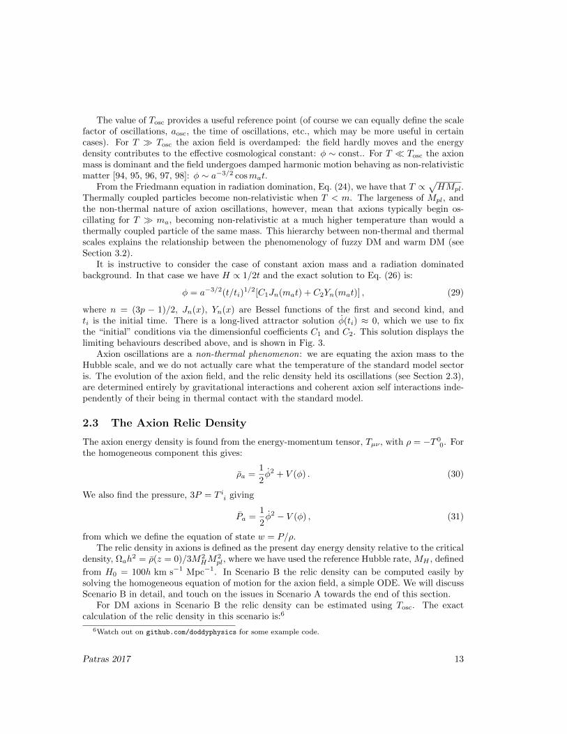
The value of Tosc provides a useful reference point (of course we can equally define the scalefactor of oscillations, aosc, the time of oscillations, etc., which may be more useful in certaincases). For T Tosc the axion field is overdamped: the field hardly moves and the energydensity contributes to the effective cosmological constant: φ ∼ const.. For T Tosc the axionmass is dominant and the field undergoes damped harmonic motion behaving as non-relativisticmatter [94, 95, 96, 97, 98]: φ ∼ a−3/2 cosmat.

From the Friedmann equation in radiation domination, Eq. (24), we have that T ∝√HMpl.

Thermally coupled particles become non-relativistic when T < m. The largeness of Mpl, andthe non-thermal nature of axion oscillations, however, mean that axions typically begin os-cillating for T ma, becoming non-relativistic at a much higher temperature than would athermally coupled particle of the same mass. This hierarchy between non-thermal and thermalscales explains the relationship between the phenomenology of fuzzy DM and warm DM (seeSection 3.2).

It is instructive to consider the case of constant axion mass and a radiation dominatedbackground. In that case we have H ∝ 1/2t and the exact solution to Eq. (26) is:

φ = a−3/2(t/ti)1/2[C1Jn(mat) + C2Yn(mat)] , (29)

where n = (3p − 1)/2, Jn(x), Yn(x) are Bessel functions of the first and second kind, andti is the initial time. There is a long-lived attractor solution φ(ti) ≈ 0, which we use to fixthe “initial” conditions via the dimensionful coefficients C1 and C2. This solution displays thelimiting behaviours described above, and is shown in Fig. 3.

Axion oscillations are a non-thermal phenomenon: we are equating the axion mass to theHubble scale, and we do not actually care what the temperature of the standard model sectoris. The evolution of the axion field, and the relic density held its oscillations (see Section 2.3),are determined entirely by gravitational interactions and coherent axion self interactions inde-pendently of their being in thermal contact with the standard model.

2.3 The Axion Relic Density

The axion energy density is found from the energy-momentum tensor, Tµν , with ρ = −T 00. For

the homogeneous component this gives:

ρa =1

2φ2 + V (φ) . (30)

We also find the pressure, 3P = T ii giving

Pa =1

2φ2 − V (φ) , (31)

from which we define the equation of state w = P/ρ.The relic density in axions is defined as the present day energy density relative to the critical

density, Ωah2 = ρ(z = 0)/3M2

HM2pl, where we have used the reference Hubble rate, MH , defined

from H0 = 100h km s−1 Mpc−1. In Scenario B the relic density can be computed easily bysolving the homogeneous equation of motion for the axion field, a simple ODE. We will discussScenario B in detail, and touch on the issues in Scenario A towards the end of this section.

For DM axions in Scenario B the relic density can be estimated using Tosc. The exactcalculation of the relic density in this scenario is:6

6Watch out on github.com/doddyphysics for some example code.

Patras 2017 13

• Find Tosc: AH(Tosc) = ma(Tosc). The choice of A is crucial: more below.

• Compute the energy density at Tosc from the (numerical) solution of the equation ofmotion for θ up to this time: ρ = f2

a θ2/2 +ma(Tosc)2f2

aU(θ).

• Redshift the number density, na = ρa/ma, as non-relativistic matter from this point on(normalising the scale factor to a(z = 0) = 1): na(z = 0) = ma(Tosc)f2

aθ2i /2a(Tosc)3. The

scale factor can be computed using conservation of entropy (see e.g. Ref. [99]).

• Compute the energy density: ρ(z = 0) = na(z = 0)ma(T0), where T0 is the temperaturetoday.

The first bullet point is key to the accuracy of the calculation. In a full numerical solutionwe should take A large enough that the field has undergone many oscillations, and that indeedwe are in the harmonic regime where na is adiabatically conserved. The reason we must makethis approximation even for numerical solutions is that for dark matter axions Tosc T0 andfollowing a large number of oscillations is numerically prohibitive. As long as A is thus chosenlarge enough, then with the numerical solution for θ the other steps are essentially exact.

For analytic approximations, we typically take A = 3 and approximate the axion energyin the second bullet point as being exactly the initial value for a quadratic potential: ρi =ma(Tosc)2f2

aθ2i /2. Making these approximations, and using the temperature evolution of the

mass consistent with the QCD axion leads to the standard formulae approximating the relicdensity that can be found in e.g. Refs. [100, 9].

Obviously the choice of A is related to matching the solutions correctly under this approxi-mation. This is demonstrated in Fig. 3, where this approximation works well for A = 2 for theconstant mass ALP in this idealised situation of pure radiation domination for the background.

In real-Universe examples with a matter-to-radiation transition and late time Λ domination,we found in Ref. [101] that A = 3 works well for a constant mass ALP with a quadratic potential.In this case, the analytic approximation for the relic density gives [102]:

Ωa ≈

16 (9Ωr)

3/4(ma

H0

)1/2⟨(

φi

Mpl

)2⟩

if aosc < aeq ,

96Ωm

⟨(φi

Mpl

)2⟩

if aeq < aosc . 1 ,

16

(ma

H0

)2⟨(

φi

Mpl

)2⟩

if aosc & 1 ,

, (32)

where φi = faθi. The angle brackets appear since in Scenario B the scale-invariant isocurvatureperturbations contribute to the mean square misalignment:

〈φ2〉 = f2aθ

2i +H2

I /(2π)2 . (33)

In Scenario B the value of θi is a free parameter we can use to set the desired relic density. Itis standard to include an “anharmonic correction factor”, fan(θ), which provides an additionalfudge factor increasing the relic density due to the delayed onset of oscillations when θ ∼ π.Fits for this can be found in e.g. Ref. [103], but nothing is a substitute for direct numericalsolution.

Fig. 4 shows contours of constant relic density from Eq. (32) for ultralight axions (ULAs).We assume a quadratic potential and take with HI = 1014 GeV.

14 Patras 2017

-24 -22 -20 -18 -16 -14 -12

14

15

16

17

18

Excluded: ah 2

>0.12

-9

-7

-5

-3

-1

log10(

ah

2)

log10(ma/eV)

log10(

i/G

eV)

Figure 4: ULA relic density from vacuum realignment in Scenario B from the analytic approx-imation Eq. (32). Reproduced from Ref. [9].

Patras 2017 15

16 14 12 10 8 6 4 2log10(ma/eV)

9

10

11

12

13

14lo

g 10(

f a/G

eV)

n = 0

n = 3.34

n = 6

Figure 5: Approximation to the relic density in Scenario A for different temperature evolutionsof the axion mass parameterised by index n. Solid and dashed lines show different values for theeffects of anharmonicities and topological defect decay, with the solid lines being the preferredvalues from Ref. [104] for defects, and my own fits to anharmonic corrections. Reproduced fromRef. [82].

It is interesting to observe in this plot that values of the decay constant that are naturalin a variety of string-inspired models, fa ∼ 1016−17 GeV, provide the correct relic density ofaxions for masses of the order ma = 10−18−22 eV. This happens to be the mass range of fuzzyDM which is accessible to tests from galaxy formation, and displays interesting signatures thatcould allow it to be distinguished from standard cold DM (see Section 3.2).

The relic density computation in Scenario A is far more involved. The full calculationrequires solving the inhomogeneous axion equation of motion, which accounts for string anddomain wall decay. For NDW = 1, these effects can be parameterised using a single rescaling ofthe homogeneous solution by (1+αdec), with the simulations of Ref. [104] favouring αdec. = 2.48for the QCD axion. In order to correctly use the rescaling, it is also necessary to use the averagevalue of the homogeneous evolution and any anharmonic corrections:

〈θ2i fan(θi)〉 =

1

2π

∫ π

−πθ2fan(θ)dθ ≡ can

π2

3. (34)

With αdec. and can. fit from simulations, the relic density can then be computed as in ScenarioB, but now with the misalignment angle fixed to θi = π/

√3. A more detailed discussion of the

calculation can be found in Ref. [82]. The results of this approximation are shown in Fig. 5.

16 Patras 2017

B

g

Figure 6: Axion-photon conversion in the presence of an external magnetic field, B. Reproducedfrom Ref. [9].

3 Axion Phenomenology

3.1 Couplings

Axion couplings to the standard model have a number of effects that allow the coupling strengthto be constrained in the lab and from astrophysics. A thorough review of all experimentalconstraints on axions is given in Ref. [105]. Global fits are presented in Ref. [106]. A review ofall constraints on the photon coupling is given in Ref. [107]. Briefly, some relevant phenomenaare:

• Stellar evolution. Axions can be produced from standard model particles inside stars.The axions are very weakly interacting and thus easily escape the stars and supernovae,offering an additional cooling channel. The physics and constraints are reviewed by Raffeltin Refs. [108, 109]. A rather robust bound comes from the ratio of horizontal branchstars to red giants found in globular clusters, which bounds the axion photon couplinggγ < 6.6 × 10−11 GeV−1 [110]. There is also the “white dwarf cooling hint” for axions:excess cooling of white dwarfs might be explained by axion emission via the couplingge [111].

• Axion mediated forces. The pseudoscalar couplings gN and ge mediate a spin-dependentforce between standard model particles [112]. Constraints on these forces in the labora-tory are not very strong compared to the bounds from stellar astrophysics [113]. How-ever, the proposed “ARIADNE” experiment using nuclear magnetic resonance will makesubstantial improvements, and could even detect the QCD axion for 109 GeV . fa .1012 GeV [114].

• “Haloscopes” and other dark matter detection techniques. Using the axion-photon inter-action, gγ , dark matter axions can be turned into photons in the presence of magneticfields (see Fig. 6) inside resonant microwave cavities [115]. The ADMX experiment isthe leader in such constraints [116], but many new proposals discussed at this conference

Patras 2017 17

will soon also enter the game, including the ADMX high frequency upgrade. Notablenew techniques that do not rely on the microwave cavity include the use of resonatingcircuits [117] and the ABRACADABRA proposal [118]; nuclear magnetic resonance andthe CASPEr proposal [119, 120]; and dielectric dish antenna and the MADMAX pro-posal [121]. Together, these proposals promise to cover almost the entire parameter spacefor QCD axion dark matter with fa . 1016 GeV. It truly is an exciting time!

• Axion decays. As noted in Eq. (13) the axion-photon interaction allows axions to decay.Heavy axions decay on cosmological time scales, and are constrained by the effects onthe CMB anisotropies, BBN, and CMB spectral distortions [122, 123, 18]. The strongestconstraint comes from the deuterium abundance. Axions and ALPs are generally excludedfor masses and lifetimes 1 keV . ma . 1 GeV and 10−4 s . τφγ . 106 s

• Axion-photon conversion in astrophysics. Magnetic fields in clusters convert photonsinto axions and alter the spectrum of the X-ray photons arriving at Earth. The non-observation of such modulations by the Chandra satellite places a bound on the axion-photon coupling gγ . 10−12 GeV−1 [124]. In cosmic magnetic fields the same phenomenoninduces CMB spectral distortions, constraining a product of the photon coupling and thecosmic magnetic field strength [125, 126]. Conversion of axions to photons in the MilkyWay magnetic field produces a background of GHz photons correlated with the magneticfield that is accessible to observation by SKA for a range of masses and couplings consistentwith QCD axion dark matter [127], and in the same range that could be detected directlyby high frequency ADMX.

• Anomalous spin precession. The axion coupling to the neutron EDM, gd, and the nucleoncoupling, gN induce spin-precession of neutrons and nuclei in the presence of the axion DMbackground field. For gd this occurs in the presence of electric and magnetic fields [43, 119].For gN this occurs in magnetic fields, with the axion DM “wind” playing the role of apseudo magnetic field [43, 128]. These effects are the basis of the CASPEr proposal, andhave been constrained directly using archival data from nEDM [129].

• “Light Shining Through a Wall”. Axions pass virtually unimpeded through materials(“walls”) that are opaque to photons. Converting a laser photon into an axion using amagnetic field, allowing it to pass through an intermediate wall, and then converting theaxion back into a photon, would allow the laser to pass through the wall and indirectlygive evidence for axions. This search technique [130] is the basis for the “ALPS” exper-iment [131, 132], which aims at constraining gφγ ∼ 2 × 10−11 GeV−1 in the upgradedversion currently in operation.

• “Helioscopes”. Axions from the sun can be converted into visible photons inside a tele-scope with a magnetic field [115]. Constraints on gγ . 10−10 GeV−1 using this techniquehave been presented by the CAST experiment [133, 134, 135]. The proposed “Interna-tional Axion Observatory” would improve the limits by an order of magnitude [136].

3.2 Gravitation

The classical axion field, φ, has novel gravitational effects caused by the Compton wavelength,and by the axion potential.

18 Patras 2017

• “Fuzzy” Dark Matter. As already discussed, when the axion mass is very small, ma ∼10−22 eV, the field displays coherence on astrophysical length scales [50, 51, 52, 53]. Thismakes ULAs distinct from cold DM, and drives the lower bound on DM particle mass fromcosmological constraints such as the CMB anisotropies [137, 101, 91], the high redshiftluminosity function [138, 139, 140], and the Lyman-α forest flux power spectrum [141,142]. Superficially the model resembles warm DM [143], suppressing cosmic structureformation below a certain length scale, and with the warm DM mass, mX , roughly relatedto the axion mass as mX ∼

√maMpl. However, the small scale physics is very different

and fuzzy DM requires dedicated simulations, which reveal striking unique features suchas soliton formation, and quasi-particles. A number of beyond-CDM simulations andsemi-analytic methods have been developed to study this novel type of DM [52, 144, 145,146, 147].

• Black hole superradiance. This gravitational phenomenon applies to all bosonic fields,with different timescales depending on the spin (zero, one, or two). A population of bosonsis built up in a “gravitational atom” around the black hole from vacuum fluctuations. Thusthis phenomenon makes no assumptions about the cosmic density or origin of the bosonicfield. Spin is extracted from the black hole via the Penrose process [148]. The boson massprovides a potential barrier (a “mirror”), and the process becomes runaway [149, 150]. Theresulting spin down of black holes makes certain regions on the “Regge plane” (mass versusspin plane) effectively forbidden for astrophysical black holes. Astrophysical observationsof rapidly rotating black holes thus exclude bosons of certain ranges of mass [151, 37, 152,153, 154]. For the spin zero axion, stellar mass black holes exclude 6× 10−13 eV < ma <2×10−11 eV at 2σ, which for the QCD axion excludes 3×1017 GeV < fa < 1×1019 GeV.The supermassive BH measurements give only 1σ exclusions 10−18 eV < ma < 10−16 eV.The energy extracted from the BH angular momentum can be emitted by the axioncloud in the form of gravitational waves (GWs). The recent direct detection of GWs byLIGO [155] opens up an exciting new opportunity to study axions and other light bosonsfrom the inferred mass and spin distributions of BHs, and from direct GW signals ofsuperradiance [156, 157].

• Oscillating dark matter pressure. The axion equation of state (shown in Fig. 3) oscil-lates with frequency 2ma, originating from an oscillating pressure. The axion is onlypressureless when averaged over time scales larger than (2ma)−1. Pressure oscillationsinduce oscillations in the metric potentials, which manifest as a scalar strain on pulsartiming arrays (PTAs) and in gravitational wave detectors (just as gravitational waves area tensor strain) [158]. The NANOGrav PTA sets limits an order of magnitude higherthan the expected signal at ma = 10−23 eV [159], though SKA is forecast to be sensitiveto the signal at this mass even if such ULAs constitute just 1% of the DM [158]. In GWdetectors, the axion DM wind anisotropic stress, σij ∝ ∇iφ∇jφ, manifests as a “scalarGW” also [160].

• Axion stars. The gradient term in the Klein Gordon equation opposes gravitationalcollapse of scalar fields on small scales. This leads to the existence of a class of pseudo-solitonic boson star known as an oscilloton [161, 162] for the case of a massive real scalar.For axions, these solutions are “axion stars”. These objects are formed during gravita-tional collapse, halted by the effective pressure of the gradients. Emission of scalar wavesleads to “gravitational cooling” [163], and the stars settle into the ground state. The soli-

Patras 2017 19

tons are a condensate of coherent axions. Axions stars are observed to form in the centresof DM halos in numerical simulations [52, 164, 146]. This density core may play a role inthe presence of cores in dwarf spheroidal satellites of the Milky Way [165, 166, 167]. Ax-ion stars should also be present in the centre of miniclusters, and, if axion self-scatteringis efficient, entire miniclusters might thus condense [73]. Axion stars have a maximummass above which they become unstable [168]. For weak self-interactions, fa & Mpl, theinstability leads to black hole formation, while for stronger self-interactions the instabil-ity results in emission of relativistic axion waves [168, 169, 170, 171, 172, 173]. Axionstars could detected as they pass through the Earth using a network of magnetome-ters [174]. Especially compact axion stars could lead to unique signatures in gravitationalwave detectors from their binary inspirals with each other and with other astrophysicalobjects [175].

• Inflation and Dark Energy. The periodic nature of the axion potential implies that thereare maxima where the potential is locally flat. The (tachyonic) mass at the maximum isprotected from perturbative quantum corrections by the shift symmetry, leading to fairlynatural models for inflation [176] and dark energy [177]. The axion potential contributesto the effective cosmological constant. If the field is placed sufficiently close to the topof the potential, then a sufficient number of e-foldings of inflation can be driven (fordark energy the requirement is instead on the equation of state). Constraints on axiondark energy can be found in Ref. [178]. The simplest model of natural inflation takesV (φ) ∝ cos(φ/fa). After normalising the scalar CMB amplitude, this model is a twoparameter family giving predicting a strip in the plane of scalar spectral index versustensor-to-scalar ratio, (ns, rT ). It is consistent with the Planck results [179], but couldcould be excluded by CMB-S4 [180]. Variants on axion inflation inspired by string theoryare N -flation [181] and axion monodromy [46, 47]. Both models seek to deal with issuesrelating to super-Planckian field excursions, the Lyth bound for rT [182], and the “weakgravity conjecture” [183], and construct string-inspired models with observably large rT .

Acknowledgements

These brief notes contributed to the 13th Patras Workshop on Axions, WIMPs and WISPs,Thessaloniki, May 15 to 19, 2017. They rely heavily on the review Ref. [9], which is far morecomplete, and from which most figures are taken (though of course these notes discuss newresults of the last two years). I am grateful to Thomas Bachlechner, Laura Covi, Jihn Kim,Chris Murphy, Maxim Pospelov, and Andreas Ringwald for useful discussions, and to VishnuJejala for providing the data for Fig. 2. Work at King’s College London was supported by aRoyal Astronomical Society Postdoctoral Fellowship. Research at the University of Gottingenis funded by the Alexander von Humboldt Foundation and the German Federal Ministry ofEducation and Research.

References

[1] R. Peccei and H. R. Quinn, Phys. Rev. Lett.38, 1440 (1977).

[2] S. Weinberg, Phys. Rev. Lett.40, 223 (1978).

[3] F. Wilczek, Phys. Rev. Lett.40, 279 (1978).

20 Patras 2017

[4] R. J. Crewther, P. di Vecchia, G. Veneziano, and E. Witten, Phys. Lett. B 88, 123 (1979).

[5] J. M. Pendlebury et al., Phys. Rev. D92, 092003 (2015), 1509.04411.

[6] K. A. Olive and Particle Data Group, Chinese Physics C 38, 090001 (2014), 1412.1408.

[7] M. Srednicki, Nucl. Phys. B260, 689 (1985).

[8] A. Zee, Quantum field theory in a nutshell (, 2003).

[9] D. J. E. Marsh, Phys. Rep.643, 1 (2016), 1510.07633.

[10] S. Coleman, Aspects of Symmetry (Cambridge University Press, 1988).

[11] C. Vafa and E. Witten, Phys. Rev. Lett.53, 535 (1984).

[12] G. G. di Cortona, E. Hardy, J. P. Vega, and G. Villadoro, Journal of High Energy Physics 1, 34 (2016),1511.02867.

[13] D. J. Gross, R. D. Pisarski, and L. G. Yaffe, Reviews of Modern Physics 53, 43 (1981).

[14] S. Borsanyi et al., Physics Letters B 752, 175 (2016), 1508.06917.

[15] S. Borsanyi et al., Nature 539, 69 (2016), 1606.07494.

[16] P. Sikivie, Phys. Rev. Lett.48, 1156 (1982).

[17] J. E. Kim, Phys. Rept. 150, 1 (1987).

[18] M. Millea, L. Knox, and B. D. Fields, Phys. Rev. D92, 023010 (2015), 1501.04097.

[19] J. E. Kim, Phys. Rev. Lett.43, 103 (1979).

[20] M. A. Shifman, A. I. Vainshtein, and V. I. Zakharov, Nuclear Physics B 166, 493 (1980).

[21] M. Dine, W. Fischler, and M. Srednicki, Phys. Lett. B 104, 199 (1981).

[22] A. Zhitnitsky, Sov.J . Nucl. Phys. 31, 260 (1980).

[23] L. Di Luzio, F. Mescia, and E. Nardi, Physical Review Letters 118, 031801 (2017), 1610.07593.

[24] P. Svrcek and E. Witten, JHEP6, 51 (2006), hep-th/0605206.

[25] J. P. Conlon, Journal of High Energy Physics 5, 078 (2006), hep-th/0602233.

[26] K. Becker, M. Becker, and J. H. Schwarz, String Theory and M-Theory (Cambridge University Press,2007).

[27] A. Ringwald, ArXiv e-prints (2012), 1209.2299.

[28] M. Cicoli, M. D. Goodsell, and A. Ringwald, JHEP10, 146 (2012), 1206.0819.

[29] S. M. Carroll, Spacetime and geometry. An introduction to general relativity (Addison Wesley, 2004).

[30] M. B. Green, J. H. Schwarz, and E. Witten, Superstring theory. Volume 2 - Loop amplitudes, anomaliesand phenomenology (Cambridge University Press, 1987).

[31] P. Candelas, G. T. Horowitz, A. Strominger, and E. Witten, Nuclear Physics B 258, 46 (1985).

[32] R. Altman, J. Gray, Y.-H. He, V. Jejjala, and B. D. Nelson, JHEP 02, 158 (2015), 1411.1418.

[33] Y.-H. He, (2017), 1706.02714.

[34] M. Kreuzer and H. Skarke, Adv. Theor. Math. Phys. 4, 1209 (2002), hep-th/0002240.

[35] M. Kreuzer and H. Skarke, ArXiv Mathematics e-prints (2000), math/0001106.

[36] T. W. Grimm and J. Louis, Nucl. Phys. B699, 387 (2004), hep-th/0403067.

[37] A. Arvanitaki, S. Dimopoulos, S. Dubovsky, N. Kaloper, and J. March-Russell, Phys. Rev. D81, 123530(2010), 0905.4720.

[38] R. Easther and L. McAllister, JCAP5, 018 (2006), hep-th/0512102.

[39] M. J. Stott, D. J. E. Marsh, C. Pongkitivanichkul, L. C. Price, and B. S. Acharya, Phys. Rev. D96,083510 (2017), 1706.03236.

[40] T. C. Bachlechner, K. Eckerle, O. Janssen, and M. Kleban, (2017), 1703.00453.

[41] S. B. Giddings and A. Strominger, Nuclear Physics B 306, 890 (1988).

[42] R. Alonso and A. Urbano, ArXiv e-prints (2017), 1706.07415.

Patras 2017 21

[43] P. W. Graham and S. Rajendran, Phys. Rev. D88, 035023 (2013), 1306.6088.

[44] A. G. Dias, A. C. B. Machado, C. C. Nishi, A. Ringwald, and P. Vaudrevange, Journal of High EnergyPhysics 6, 37 (2014), 1403.5760.

[45] J. E. Kim and D. J. E. Marsh, Phys. Rev. D93, 025027 (2016), 1510.01701.

[46] E. Silverstein and A. Westphal, Phys. Rev. D78, 106003 (2008), 0803.3085.

[47] L. McAllister, E. Silverstein, and A. Westphal, Phys. Rev. D82, 046003 (2010), 0808.0706.

[48] M. Kamionkowski and J. March-Russell, Physics Letters B 282, 137 (1992), hep-th/9202003.

[49] R. Kallosh, A. Linde, D. Linde, and L. Susskind, Phys. Rev. D52, 912 (1995), hep-th/9502069.

[50] W. Hu, R. Barkana, and A. Gruzinov, Physical Review Letters 85, 1158 (2000), astro-ph/0003365.

[51] D. J. E. Marsh and J. Silk, MNRAS437, 2652 (2014), 1307.1705.

[52] H.-Y. Schive, T. Chiueh, and T. Broadhurst, Nature Physics 10, 496 (2014), 1406.6586.

[53] L. Hui, J. P. Ostriker, S. Tremaine, and E. Witten, Phys. Rev. D95, 043541 (2017), 1610.08297.

[54] J. P. Conlon and M. C. D. Marsh, Phys. Rev. Lett.111, 151301 (2013), 1305.3603.

[55] J. P. Conlon and M. C. D. Marsh, JHEP10, 214 (2013), 1304.1804.

[56] L. Iliesiu, D. J. E. Marsh, K. Moodley, and S. Watson, Phys. Rev. D89, 103513 (2014), 1312.3636.

[57] M. Archidiacono, S. Hannestad, A. Mirizzi, G. Raffelt, and Y. Y. Y. Wong, JCAP10, 020 (2013),1307.0615.

[58] E. Di Valentino, S. Gariazzo, E. Giusarma, and O. Mena, Phys. Rev. D91, 123505 (2015), 1503.00911.

[59] E. Di Valentino et al., Physics Letters B 752, 182 (2016), 1507.08665.

[60] S. Hannestad, A. Mirizzi, and G. Raffelt, JCAP7, 002 (2005), hep-ph/0504059.

[61] S. Hannestad, A. Mirizzi, G. G. Raffelt, and Y. Y. Y. Wong, JCAP8, 015 (2007), 0706.4198.

[62] S. Hannestad, A. Mirizzi, G. G. Raffelt, and Y. Y. Y. Wong, JCAP4, 019 (2008), 0803.1585.

[63] S. Hannestad, A. Mirizzi, G. G. Raffelt, and Y. Y. Y. Wong, JCAP8, 001 (2010), 1004.0695.

[64] O. Wantz and E. Shellard, Phys. Rev. D82, 123508 (2010), 0910.1066.

[65] G. Ballesteros, J. Redondo, A. Ringwald, and C. Tamarit, JCAP8, 001 (2017), 1610.01639.

[66] R. L. Davis, Phys. Rev. D32, 3172 (1985).

[67] D. Harari and P. Sikivie, Phys. Lett. B 195, 361 (1987).

[68] R. A. Battye and E. P. S. Shellard, Phys. Rev. Lett.73, 2954 (1994), astro-ph/9403018.

[69] R. A. Battye and E. P. S. Shellard, Phys. Rev. Lett.76, 2203 (1996).

[70] T. Hiramatsu, M. Kawasaki, K. Saikawa, and T. Sekiguchi, Phys. Rev. D85, 105020 (2012), 1202.5851.

[71] V. B. Klaer and G. D. Moore, ArXiv e-prints (2017), 1708.07521.

[72] C. J. Hogan and M. J. Rees, Phys. Lett. B 205, 228 (1988).

[73] E. W. Kolb and I. I. Tkachev, Phys. Rev. Lett.71, 3051 (1993), hep-ph/9303313.

[74] E. W. Kolb and I. I. Tkachev, Phys. Rev. D49, 5040 (1994), astro-ph/9311037.

[75] E. W. Kolb and I. I. Tkachev, Phys. Rev. D50, 769 (1994), astro-ph/9403011.

[76] E. W. Kolb and I. I. Tkachev, ApJLett460, L25 (1996), astro-ph/9510043.

[77] K. M. Zurek, C. J. Hogan, and T. R. Quinn, Phys. Rev. D75, 043511 (2007), astro-ph/0607341.

[78] E. Hardy, Journal of High Energy Physics 2, 46 (2017), 1609.00208.

[79] M. Fairbairn, D. J. E. Marsh, and J. Quevillon, Phys. Rev. Lett. 119, 021101 (2017), 1701.04787.

[80] C. A. J. O’Hare and A. M. Green, Phys. Rev. D95, 063017 (2017), 1701.03118.

[81] P. Tinyakov, I. Tkachev, and K. Zioutas, JCAP1, 035 (2016), 1512.02884.

[82] M. Fairbairn, D. J. E. Marsh, J. Quevillon, and S. Rozier, (2017), 1707.03310.

[83] I. I. Tkachev, JETP Lett. 101, 1 (2015), 1411.3900, [Pisma Zh. Eksp. Teor. Fiz.101,no.1,3(2015)].

22 Patras 2017

[84] A. Iwazaki, (2017), 1707.04827.

[85] A. Iwazaki, (2014), 1412.7825.

[86] E. Komatsu et al., ApJS180, 330 (2009), 0803.0547.

[87] Planck Collaboration et al., A&A594, A20 (2016), 1502.02114.

[88] M. P. Hertzberg, M. Tegmark, and F. Wilczek, Phys. Rev. D78, 083507 (2008), 0807.1726.

[89] D. J. E. Marsh, D. Grin, R. Hlozek, and P. G. Ferreira, Physical Review Letters 113, 011801 (2014).

[90] L. Visinelli and P. Gondolo, Phys. Rev. Lett.113, 011802 (2014), 1403.4594.

[91] R. Hlozek, D. J. E. Marsh, and D. Grin, (2017), 1708.05681.

[92] Planck Collaboration et al., A&A594, A13 (2016), 1502.01589.

[93] BICEP2 Collaboration et al., Phys. Rev. Lett.116, 031302 (2016), 1510.09217.

[94] J. Preskill, M. B. Wise, and F. Wilczek, Phys. Lett. B 120, 127 (1983).

[95] M. Dine and W. Fischler, Phys. Lett. B 120, 137 (1983).

[96] L. F. Abbott and P. Sikivie, Phys. Lett. B 120, 133 (1983).

[97] P. J. Steinhardt and M. S. Turner, Phys. Lett. B 129, 51 (1983).

[98] M. S. Turner, Phys. Rev. D28, 1243 (1983).

[99] E. W. Kolb and M. S. Turner, The early universe. (Addison-Wesley, 1990).

[100] P. Fox, A. Pierce, and S. Thomas, ArXiv High Energy Physics - Theory e-prints (2004), hep-th/0409059.

[101] R. Hlozek, D. Grin, D. J. E. Marsh, and P. G. Ferreira, Phys. Rev. D91, 103512 (2015), 1410.2896.

[102] D. J. E. Marsh and P. G. Ferreira, Phys. Rev. D82, 103528 (2010), 1009.3501.

[103] A. Diez-Tejedor and D. J. E. Marsh, (2017), 1702.02116.

[104] M. Kawasaki, K. Saikawa, and T. Sekiguchi, Phys. Rev. D91, 065014 (2015), 1412.0789.

[105] P. W. Graham, I. G. Irastorza, S. K. Lamoreaux, A. Lindner, and K. A. van Bibber, Annual Review ofNuclear and Particle Science 65, 485 (2015), 1602.00039.

[106] GAMBIT, S. Hoof, A Preview of Global Fits of Axion Models in GAMBIT, in 13th Patras Workshop onAxions, WIMPs and WISPs (AXION-WIMP 2017) CHALKIDIKI TBC, GREECE, May 15-19, 2017,2017, 1710.11138.

[107] G. Carosi et al., ArXiv e-prints (2013), 1309.7035.

[108] G. G. Raffelt, Phys. Rept. 198, 1 (1990).

[109] G. G. Raffelt, Astrophysical Axion Bounds, in Axions, edited by M. Kuster, G. Raffelt, and B. Beltran,, Lecture Notes in Physics, Berlin Springer Verlag Vol. 741, p. 51, 2008, hep-ph/0611350.

[110] A. Ayala, I. Domınguez, M. Giannotti, A. Mirizzi, and O. Straniero, Phys. Rev. Lett.113, 191302 (2014),1406.6053.

[111] J. Isern, White dwarfs as physics laboratories: the case of axions, in 7th Patras Workshop on Axions,WIMPs and WISPs (PATRAS 2011), edited by K. Zioutas and M. Schumann, p. 158, 2012, 1204.3565.

[112] J. Moody and F. Wilczek, Phys. Rev. D30, 130 (1984).

[113] G. Raffelt, Phys. Rev. D86, 015001 (2012), 1205.1776.

[114] A. Arvanitaki and A. A. Geraci, Phys. Rev. Lett.113, 161801 (2014), 1403.1290.

[115] P. Sikivie, Phys. Rev. Lett.51, 1415 (1983).

[116] S. J. Asztalos et al., Phys. Rev. Lett.104, 041301 (2010), 0910.5914.

[117] P. Sikivie, N. Sullivan, and D. B. Tanner, Phys. Rev. Lett.112, 131301 (2014), 1310.8545.

[118] Y. Kahn, B. R. Safdi, and J. Thaler, Physical Review Letters 117, 141801 (2016), 1602.01086.

[119] D. Budker, P. W. Graham, M. Ledbetter, S. Rajendran, and A. O. Sushkov, Phys. Rev. X 4, 021030(2014), 1306.6089.

[120] A. Garcon et al., ArXiv e-prints (2017), 1707.05312.

[121] MADMAX Working Group, A. Caldwell et al., Phys. Rev. Lett.118, 091801 (2017), 1611.05865.

Patras 2017 23

[122] J. Ellis, G. B. Gelmini, J. L. Lopez, D. V. Nanopoulos, and S. Sarkar, Nuclear Physics B 373, 399 (1992).

[123] E. Masso and R. Toldra, Phys. Rev. D55, 7967 (1997), hep-ph/9702275.

[124] J. P. Conlon, F. Day, N. Jennings, S. Krippendorf, and M. Rummel, JCAP7, 005 (2017), 1704.05256.

[125] A. Mirizzi, J. Redondo, and G. Sigl, JCAP8, 1 (2009), 0905.4865.

[126] H. Tashiro, J. Silk, and D. J. E. Marsh, Phys. Rev. D88, 125024 (2013), 1308.0314.

[127] K. Kelley and P. J. Quinn, ApJLett845, L4 (2017), 1708.01399.

[128] V. Flambaum, 9th Patras Workshop (2013).

[129] C. Abel et al., Phys. Rev. X7, 041034 (2017), 1708.06367.

[130] J. Redondo and A. Ringwald, Contemporary Physics 52, 211 (2011), 1011.3741.

[131] K. Ehret et al., Physics Letters B 689, 149 (2010), 1004.1313.

[132] R. Bahre et al., Journal of Instrumentation 8, 9001 (2013), 1302.5647.

[133] K. Zioutas et al., Phys. Rev. Lett.94, 121301 (2005), hep-ex/0411033.

[134] S. Andriamonje et al., JCAP4, 10 (2007), hep-ex/0702006.

[135] M. Arik et al., Phys. Rev. Lett.112, 091302 (2014), 1307.1985.

[136] J. K. Vogel et al., IAXO - The International Axion Observatory, in 8th Patras Workshop on Axions,WIMPs and WISPs (AXION-WIMP 2012) Chicago, Illinois, July 18-22, 2012, 2013, 1302.3273.

[137] L. Amendola and R. Barbieri, Physics Letters B 642, 192 (2006), hep-ph/0509257.

[138] B. Bozek, D. J. E. Marsh, J. Silk, and R. F. G. Wyse, MNRAS450, 209 (2015), 1409.3544.

[139] H.-Y. Schive, T. Chiueh, T. Broadhurst, and K.-W. Huang, ApJ818, 89 (2016), 1508.04621.

[140] P. S. Corasaniti, S. Agarwal, D. J. E. Marsh, and S. Das, Phys. Rev. D95, 083512 (2017), 1611.05892.

[141] V. Irsic, M. Viel, M. G. Haehnelt, J. S. Bolton, and G. D. Becker, Physical Review Letters 119, 031302(2017), 1703.04683.

[142] E. Armengaud, N. Palanque-Delabrouille, C. Yeche, D. J. E. Marsh, and J. Baur, MNRAS471, 4606(2017), 1703.09126.

[143] P. Bode, J. P. Ostriker, and N. Turok, ApJ556, 93 (2001), astro-ph/0010389.

[144] J. Veltmaat and J. C. Niemeyer, Phys. Rev. D94, 123523 (2016), 1608.00802.

[145] X. Du, C. Behrens, and J. C. Niemeyer, MNRAS465, 941 (2017), 1608.02575.

[146] B. Schwabe, J. C. Niemeyer, and J. F. Engels, Phys. Rev. D94, 043513 (2016), 1606.05151.

[147] P. Mocz et al., MNRAS471, 4559 (2017), 1705.05845.

[148] R. Penrose, Nuovo Cimento Rivista Serie 1, 252 (1969).

[149] W. H. Press and S. A. Teukolsky, Nature238, 211 (1972).

[150] W. H. Press and S. A. Teukolsky, ApJ185, 649 (1973).

[151] A. Arvanitaki, M. Baryakhtar, and X. Huang, Phys. Rev. D91, 084011 (2015), 1411.2263.

[152] A. Arvanitaki and S. Dubovsky, Phys. Rev. D83, 044026 (2011), 1004.3558.

[153] P. Pani, V. Cardoso, L. Gualtieri, E. Berti, and A. Ishibashi, Phys. Rev. Lett.109, 131102 (2012),1209.0465.

[154] R. Brito, V. Cardoso, and P. Pani, Classical and Quantum Gravity 32, 134001 (2015), 1411.0686.

[155] B. P. Abbott et al., Physical Review Letters 116, 061102 (2016), 1602.03837.

[156] A. Arvanitaki, M. Baryakhtar, S. Dimopoulos, S. Dubovsky, and R. Lasenby, Phys. Rev. D95, 043001(2017), 1604.03958.

[157] R. Brito et al., Phys. Rev. D96, 064050 (2017), 1706.06311.

[158] A. Khmelnitsky and V. Rubakov, JCAP2, 019 (2014), 1309.5888.

[159] N. K. Porayko and K. A. Postnov, Phys. Rev. D90, 062008 (2014), 1408.4670.

[160] A. Aoki and J. Soda, International Journal of Modern Physics D 26, 1750063 (2017), 1608.05933.

24 Patras 2017

[161] R. Ruffini and S. Bonazzola, Physical Review 187, 1767 (1969).

[162] E. Seidel and W.-M. Suen, Phys. Rev. Lett.66, 1659 (1991).

[163] E. Seidel and W.-M. Suen, Phys. Rev. Lett.72, 2516 (1994), gr-qc/9309015.

[164] H.-Y. Schive et al., Phys. Rev. Lett.113, 261302 (2014), 1407.7762.

[165] D. J. E. Marsh and A.-R. Pop, MNRAS451, 2479 (2015), 1502.03456.

[166] A. X. Gonzalez-Morales, D. J. E. Marsh, J. Penarrubia, and L. A. Urena-Lopez, MNRAS472, 1346 (2017),1609.05856.

[167] S.-R. Chen, H.-Y. Schive, and T. Chiueh, MNRAS468, 1338 (2017), 1606.09030.

[168] T. Helfer et al., JCAP3, 055 (2017), 1609.04724.

[169] D. G. Levkov, A. G. Panin, and I. I. Tkachev, Physical Review Letters 118, 011301 (2017), 1609.03611.

[170] P.-H. Chavanis, Phys. Rev. D94, 083007 (2016), 1604.05904.

[171] J. Eby, P. Suranyi, and L. C. R. Wijewardhana, Modern Physics Letters A 31, 1650090 (2016), 1512.01709.

[172] P.-H. Chavanis, ArXiv e-prints (2017), 1710.06268.

[173] J. Eby, M. Leembruggen, P. Suranyi, and L. C. R. Wijewardhana, Journal of High Energy Physics 12, 66(2016), 1608.06911.

[174] D. F. J. Kimball et al., ArXiv e-prints (2017), 1710.04323.

[175] G. F. Giudice, M. McCullough, and A. Urbano, JCAP10, 001 (2016), 1605.01209.

[176] K. Freese, J. A. Frieman, and A. V. Olinto, Phys. Rev. Lett.65, 3233 (1990).

[177] J. A. Frieman, C. T. Hill, A. Stebbins, and I. Waga, Phys. Rev. Lett.75, 2077 (1995), astro-ph/9505060.

[178] V. Smer-Barreto and A. R. Liddle, JCAP1, 023 (2017), 1503.06100.

[179] Planck Collaboration et al., AAP 594, A20 (2016), 1502.02114.

[180] K. N. Abazajian et al., ArXiv e-prints (2016), 1610.02743.

[181] S. Dimopoulos, S. Kachru, J. McGreevy, and J. G. Wacker, JCAP8, 3 (2008), hep-th/0507205.

[182] D. H. Lyth, Phys. Rev. Lett.78, 1861 (1997), hep-ph/9606387.

[183] N. Arkani-Hamed, L. Motl, A. Nicolis, and C. Vafa, JHEP6, 60 (2007), hep-th/0601001.

Patras 2017 25